XFlow: A Solution-Adaptive Code - Cenaero · PDF fileXFlow: A Solution-Adaptive Code Krzysztof...
43
XFlow: A Solution-Adaptive Code Krzysztof J. Fidkowski, University of Michigan 4 th International Workshop on High-Order CFD Methods Crete, Greece June 4-5, 2016
Transcript of XFlow: A Solution-Adaptive Code - Cenaero · PDF fileXFlow: A Solution-Adaptive Code Krzysztof...

XFlow: A Solution-Adaptive Code
Krzysztof J. Fidkowski, University of Michigan
4th International Workshop on High-Order CFD MethodsCrete, Greece
June 4-5, 2016
Code features
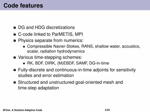
DG and HDG discretizationsC-code linked to ParMETIS, MPIPhysics separate from numerics:
Compressible Navier-Stokes, RANS, shallow water, acoustics,scalar, radiation hydrodynamics
Various time-stepping schemes:RK, BDF, DIRK, (M)EBDF, SAMF, DG-in-time
Fully-discrete and continuous-in-time adjoints for sensitivitystudies and error estimationStructured and unstructured goal-oriented mesh andtime-step adaptation
XFlow: A Solution-Adaptive Code 2/25

A typical output-adaptive result
adaptive iterations
±ε (error est.)
output
cost (degrees of freedom)
raw output
correctedoutput
exact output value
Initial mesh
Adapted mesh
XFlow: A Solution-Adaptive Code 3/25

Output-based adaptation is not always intuitive
Fishtail shock in M∞ = 0.95 inviscid flow over a NACA 0012 airfoil
500 1000 1500 20000.11
0.1105
0.111
0.1115
0.112
Number of elements
Dra
g c
oeffic
ient
exact
Mach number x-momentum adjointAdapted using drag adjoint
Adapted using residual
XFlow: A Solution-Adaptive Code 4/25

The discontinuous Galerkin method
State vector: u = [ρ, ρui, ρE, ρν]T
PDE: ∂tu +∇ · ~F(u,∇u) + S(u,∇u) = 0
Solution approximation on element e: uh(~x)∣∣∣e≈∑n(p)
j=1 Uejφj(~x)
uh ∈ Vh = [Vh]s, Vh =
u ∈ L2(Ω) : u|Ωe ∈ Pp(Ωe) ∀Ωe ∈ Th
element edomain Ω
Ωe xy
TH
u(x, y)
Ne = # of elementsn(p) = # of basis fcns
p = solution approximation orderφj(~x) = jth basis function
XFlow: A Solution-Adaptive Code 5/25

Nonlinear solver
Newton-Raphson + pseudo-time continuationLinear system at each nonlinear iteration:(
M∆ta
+∂R∂U
∣∣∣U0
)∆U + R(U0) = 0,
U0 = initial guess, M = mass matrix,∆ta is an artificial time step,
∆ta = CFL h/cmax
h = volume/(surface area), cmax = max characteristic speedover quadrature points of the elementState update is under-relaxed, U = U0 + ω∆U, to keep itphysical, via a line search
XFlow: A Solution-Adaptive Code 6/25

Wall distance calculation
SA model requires d = distance to closest wallStore d via order pwd approximation on each elementCompute d at each order pwd Lagrange node via brute forcesearch to identify closest face, projection to faceted facerepresentation, and snapping to the true geometry
actual wallcalculatedwall distance distance
point of interest
sp
s = 2/3
s = 1s = 0
s = 1/3
position on faces = reference space
linear facets
curved face
calculation on curved elements contours of wall distance
XFlow: A Solution-Adaptive Code 7/25

Output sensitivity to residuals: the adjoint
The lift adjoint Ψ is the sensitivity of lift to residual sources.
We have a solution U when R = 0
element e
Lift= J(U)
state U
Lift= J(U)
U
We have a solution U when R = 0
element e
What if we add a residual source, δRe?
δRe
Lift= J(U) + δJ
element e
U + δUWhat if we add a residual source, δRe?
We have a solution U when R = 0
resolving for the state ...
δRe
Lift= J(U) + δJ
element e
U + δUWhat if we add a residual source, δRe?
resolving for the state ...
We have a solution U when R = 0
ΨeδRe
δJ = ΨTe δRe
XFlow: A Solution-Adaptive Code 8/25
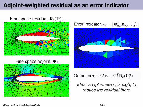
Adjoint-weighted residual as an error indicator
Fine space residual, Rh(UHh )
Fine space adjoint, Ψh
Error indicator, εe = |ΨTh,eRh,e(UH
h )|
Output error: δJ ≈ −ΨTh Rh(UH
h )
Idea: adapt where εe is high, toreduce the residual there
XFlow: A Solution-Adaptive Code 9/25
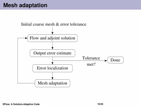
Mesh adaptation
Flow and adjoint solution
Done
Mesh adaptation
Initial coarse mesh & error tolerance
Output error estimate
Error localization
Tolerance
met?
XFlow: A Solution-Adaptive Code 10/25

h/p adaptive runs
Transonic RANS flow over a NACA 0012
XFlow: A Solution-Adaptive Code 11/25

h/p adaptive runs
DPW V
XFlow: A Solution-Adaptive Code 12/25

h/p adaptive runs
Staggered pitching/plunging airfoils; ALE, dynamic p
XFlow: A Solution-Adaptive Code 13/25
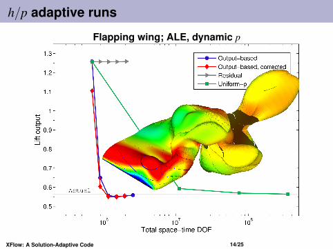
h/p adaptive runs
Flapping wing; ALE, dynamic p
XFlow: A Solution-Adaptive Code 14/25
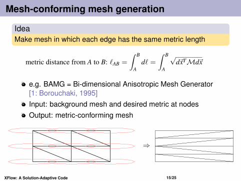
Mesh-conforming mesh generation
IdeaMake mesh in which each edge has the same metric length
metric distance from A to B: `AB =
∫ B
Ad` =
∫ B
A
√d~xTMd~x
e.g. BAMG = Bi-dimensional Anisotropic Mesh Generator[1: Borouchaki, 1995]Input: background mesh and desired metric at nodesOutput: metric-conforming mesh
⇒
XFlow: A Solution-Adaptive Code 15/25

A mesh optimization algorithm [3: Yano, 2012]
Given: current mesh, primal and adjoint solutionsDetermine: metric step matrix, Sv, at each mesh vertex, v,that produces a mesh with the smallest output error at a fixedsolution costKey ingredients
1 Error convergence model: Sv → output error2 Cost model: Sv → solution cost3 Iterative algorithm that equidistributes the marginal
error-to-cost ratio
Expect multiple iterations of optimization until error “bottomsout” at a fixed cost; can then increase allowable cost tofurther reduce error
XFlow: A Solution-Adaptive Code 16/25

Combining adaptation and optimization
1 Start with a coarse mesh at a certain cost = dof
2 Run multiple (∼ 10) mesh optimization iterations at fixed costEach iteration requires primal and adjoint solvesSolves are quick since starting from good initial guessesError will drop, then stagnate/oscillateUse results from final run or average of last few runs
increase dof
solution iteration10 200
log(error) log(dof)
3 Increase dof cost by a prescribed factor if need moreaccuracy and can afford more cost; return to step 2
XFlow: A Solution-Adaptive Code 17/25

Example: NACA 0012 in inviscid flow
Euler equations, M∞ = 0.5, α = 2, γ = 1.4, output = drag
Mach number contours
XFlow: A Solution-Adaptive Code 18/25

Example: NACA 0012 in inviscid flow
Euler equations, M∞ = 0.5, α = 2, γ = 1.4, output = drag
Initial mesh: 356 triangles, farfield @2000c
XFlow: A Solution-Adaptive Code 18/25
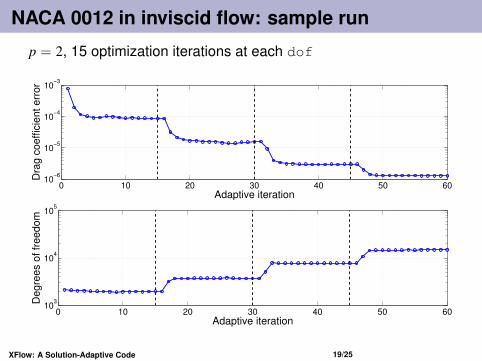
NACA 0012 in inviscid flow: sample run
p = 2, 15 optimization iterations at each dof
0 10 20 30 40 50 6010
−6
10−5
10−4
10−3
Adaptive iteration
Dra
g c
oe
ffic
ien
t e
rro
r
0 10 20 30 40 50 6010
3
104
105
Adaptive iteration
Degre
es o
f fr
eedom
XFlow: A Solution-Adaptive Code 19/25

NACA 0012 in inviscid flow: output convergence
Compare to uniform refinement at different orders p
10−2
10−8
10−7
10−6
10−5
10−4
10−3
10−2
10−1
1/sqrt(dof)
Dra
g c
oeffic
ient err
or
Optimized: p=1Optimized: p=2Optimized: p=3Uniform: p=1Uniform: p=2Uniform: p=3
XFlow: A Solution-Adaptive Code 20/25

NACA 0012 in inviscid flow: optimized meshes
p = 1, dof = 2000 p = 1, dof = 4000
p = 1, dof = 8000 p = 1, dof = 16000
XFlow: A Solution-Adaptive Code 21/25

NACA 0012 in inviscid flow: optimized meshes
p = 2, dof = 2000 p = 2, dof = 4000
p = 2, dof = 8000 p = 2, dof = 16000
XFlow: A Solution-Adaptive Code 21/25

NACA 0012 in inviscid flow: optimized meshes
p = 3, dof = 2000 p = 3, dof = 4000
p = 3, dof = 8000 p = 3, dof = 16000
XFlow: A Solution-Adaptive Code 21/25
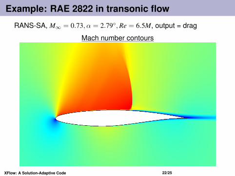
Example: RAE 2822 in transonic flow
RANS-SA, M∞ = 0.73, α = 2.79,Re = 6.5M, output = drag
Mach number contours
XFlow: A Solution-Adaptive Code 22/25

Example: RAE 2822 in transonic flow
RANS-SA, M∞ = 0.73, α = 2.79,Re = 6.5M, output = drag
Initial mesh: 758 triangles, farfield @2000c
XFlow: A Solution-Adaptive Code 22/25

RAE 2822 in transonic flow: sample run
p = 2, 15 optimization iterations at each dof
0 10 20 30 40 50 6010
−6
10−4
10−2
Adaptive iteration
Dra
g c
oe
ffic
ien
t e
rro
r
0 10 20 30 40 50 6010
3
104
105
Adaptive iteration
Degre
es o
f fr
eedom
XFlow: A Solution-Adaptive Code 23/25

RAE 2822 in transonic flow: output convergence
Compare to uniform refinement at different orders p
10−3
10−2
10−7
10−6
10−5
10−4
10−3
10−2
10−1
1/sqrt(dof)
Dra
g c
oeffic
ient err
or
Optimized: p=1Optimized: p=2Optimized: p=3Uniform: p=1Uniform: p=2Uniform: p=3
XFlow: A Solution-Adaptive Code 24/25

RAE 2822 in transonic flow: optimized meshes
p = 1, dof = 5000 p = 1, dof = 10000
p = 1, dof = 20000 p = 1, dof = 40000
XFlow: A Solution-Adaptive Code 25/25

RAE 2822 in transonic flow: optimized meshes
p = 2, dof = 5000 p = 2, dof = 10000
p = 2, dof = 20000 p = 2, dof = 40000
XFlow: A Solution-Adaptive Code 25/25
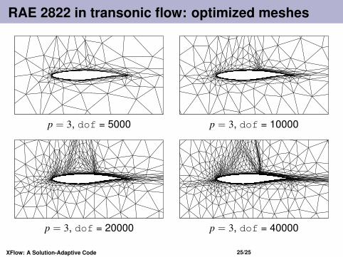
RAE 2822 in transonic flow: optimized meshes
p = 3, dof = 5000 p = 3, dof = 10000
p = 3, dof = 20000 p = 3, dof = 40000
XFlow: A Solution-Adaptive Code 25/25

Backup Slides
XFlow: A Solution-Adaptive Code 26/25

Basis choice and DG system
What basis functions to use?DG⇒ φj not tied to element shapeWe can use full-order (tri) basis on quad elementse.g. p = 4: 25 dofs for quad basis, 15 dofs for tri basis
We lump all residuals and states into single vectors (size N),
R(U) = 0
state approx.coefficients for
basis function nelement e andU = element e
Ue1Ue2
UeNpe
Uen basis fcn n ...U2
Us
U1
numbers needed to describe s order ppolynomials inside element e
XFlow: A Solution-Adaptive Code 27/25

Nonlinear solver: line search
1 Given: U0 and ∆U.2 Compute ωphys = maximum fraction such that U0 + ωphys∆U
remains physical. This involves checks at quadrature pointsof each element.
3 Set ω = min(1, ωphys). If ω < 1, set ω = ωβphys, βphys < 1.4 While ω > ωmin and ‖R(U0 + ω∆U)‖ > βresidual‖R(U0)‖: set
w = wβline, where βline < 1.5 If ω < ωmin, do not update, and set CFL = CFLβCFL,decrease.6 If ω ≥ ωmin, take the update: U = U0 + ω∆U, and if ω = 1,
raise the CFL: CFL = CFLβCFL,increase.
Parameters:
βphys = 0.5, βresidual = 2.0, βline = 0.5, ωmin = 0.24,
βCFL,increase = 1.2, βCFL,decrease = 0.1.
XFlow: A Solution-Adaptive Code 28/25

Output error estimation
We want: δJ = JH(UH)− J(U)
This is the difference between J computed with the discretesystem solution, UH, and J computed with the exact solution, U
We’ll settle for: δJ = JH(UH)− Jh(Uh)
This is the difference in J relative to a finer discretization (h)
coarse space: → RH(UH) = 0︸ ︷︷ ︸NH equations
→ UH︸︷︷︸state ∈ RNH
→ JH(UH)︸ ︷︷ ︸output (scalar)
fine space: → Rh(Uh) = 0︸ ︷︷ ︸Nh equations
→ Uh︸︷︷︸state ∈ RNh
→ Jh(Uh)︸ ︷︷ ︸output (scalar)
XFlow: A Solution-Adaptive Code 29/25

The adjoint-weighted residual
UHh solves a perturbed fine-space problem
find U′h such that: Rh(U′h)−Rh(UHh )︸ ︷︷ ︸
δRh
= 0 ⇒ answer: U′h = UHh
The fine-space adjoint, Ψh, (p + 1, solved exactly) then tellsus to expect an output perturbation of
Jh(UHh )− Jh(Uh)︸ ︷︷ ︸≈ δJ
= ΨTh δRh = −ΨT
h Rh(UHh )
This equation assumes small perturbations (e.g. if nonlinear;linearization is about UH
h )In summary, we have an adjoint-weighted residual:
δJ ≈ −ΨTh Rh(UH
h )
XFlow: A Solution-Adaptive Code 30/25
Mesh adaptation using a metric field
Unstructured meshes offer more geometric and adaptiveflexibility over structured onesResolution information: size and shape of an elementThis can be encoded in a metric field [1: Borouchaki, 1995][2: Pennec, 2006] over the domainWe are interested in an adaptive method where the mesh isregenerated at each iteration using the current mesh andinformation from the solutionKey ingredients:
1 Metric-conforming mesh generator2 Solution-based metric specification
XFlow: A Solution-Adaptive Code 31/25
Error convergence model
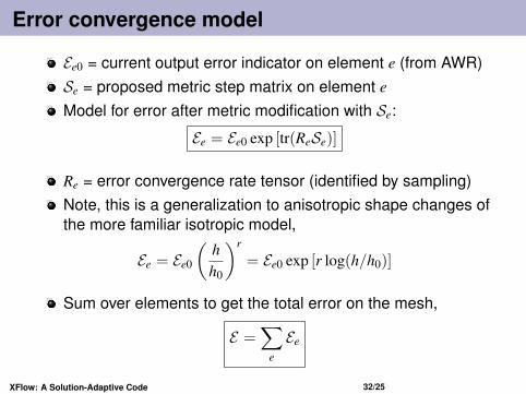
Ee0 = current output error indicator on element e (from AWR)Se = proposed metric step matrix on element e
Model for error after metric modification with Se:
Ee = Ee0 exp [tr(ReSe)]
Re = error convergence rate tensor (identified by sampling)Note, this is a generalization to anisotropic shape changes ofthe more familiar isotropic model,
Ee = Ee0
(hh0
)r
= Ee0 exp [r log(h/h0)]
Sum over elements to get the total error on the mesh,
E =∑
e
Ee
XFlow: A Solution-Adaptive Code 32/25

Cost model
cost = degrees of freedom (dof) in solution approximation
Assume p = approximation order = same for all elementsCe0 = current cost on element e, e.g. (p + 1)(p + 2)/2New cost after application of step matrix Se,
Ce = Ce0 exp[
12
tr(Se)
]︸ ︷︷ ︸
Area0/Area
Note, the cost is just scaled by Area0/Area = # new elementsoccupying the original area of element eSum over elements to get the total cost on the mesh,
C =∑
e
Ce
XFlow: A Solution-Adaptive Code 33/25

References I
[1] H. Borouchaki, P. George, F. Hecht, P. Laug, and E Saltel.Mailleur bidimensionnel de Delaunay gouverné par une carte de métriques. Partie I: Algorithmes.INRIA-Rocquencourt, France. Tech Report No. 2741, 1995.
[2] Xavier Pennec, Pierre Fillard, and Nicholas Ayache.A riemannian framework for tensor computing.International Journal of Computer Vision, 66(1):41–66, 2006.
[3] Masayuki Yano.An Optimization Framework for Adaptive Higher-Order Discretizations of Partial Differential Equations on AnisotropicSimplex Meshes.PhD thesis, Massachusetts Institute of Technology, Cambridge, Massachusetts, 2012.
XFlow: A Solution-Adaptive Code 34/25