CONVERGENCE OF DEMAND PULL INTO COST PUSH INFLATION IN INDIAN ECONOMY

Shri Prakash1 and Sudhi Sharma2

ABSTRACT

The paper focuses on inflation in Indian economy; it answers the following research questions: (i) Is inflation in India monetary or structural? (ii) Does inflation occur simultaneously in the entire Indian economy? (iii) Does RBI’s policy focus on the cause of Indian inflation? (iv) Do food/agricultural prices affect prices of manufactures? (v) Is Demand Pull inflation induced by excess money supply or decline of output of agriculture? The paper uses four Input-Output models to answer these questions in theoretical framework of flex-fix prices. Input-Output table of 2008 and 2011-12 and 2013 price is the data base. Effect of changes in 41 flex-prices on 89 fix prices is analyzed to compare results of decomposed and integrated models.

Prices of agricultural goods, especially food items rise due to crop failures which affect all other prices in the economy. Thus, demand pull food inflation converges to cost push inflation, which envelops entire economy through inter-sector linkages, rising nominal wages and inflationary expectations Food inflation spreads in entire economy since 45% of all households’ budgets and 85-86 of total expenditure of the poor is absorbed by food, about 50% of total workforce is engaged in agriculture and related activities whose incomes fall with the fall in agricultural output. But inflation does not occur in all sectors of Indian economy simultaneously; it follows lead-lag pattern.

Elasticity of fix with respect to flex prices is derived from alternative scenarios based on different rates of increase in flex-prices. Arc elasticity derived from different points’ elasticity of fix with respect to flex-prices is stable over the entire range of changes. These are methodological and theoretical innovations. Findings support the thesis that food inflation is structural which envelops non-food sectors in a lead-lag fashion. Inflation is, therefore, structural rather than monetary in India. Prices of manufactures are determined by long run average cost. But prices of agricultural goods depend on flow and stock demand of intermediate traders. Traders’ Stocking Behavior depend future expectations of agricultural prices. These traders determine prices, while traders of manufactures take prices as given, they act as commission agents. This dichotomous behavior and lead lag relation of flex-fix prices underlies food and general inflation in India.

Key-Words: Inflation, Flex-Fix Prices, Input-Output, Decomposed, Integrated Models, Intermediate Traders

___________________________________________

1. Professor of Eminence, BIMTECH, Knowledge Park II, Greater Noida, Indiashri1j38@gmail.com

2. Research Scholar, BIMTECH, Knowledge Park II, Greater Noida, IndiaSudhisharma1983@gmail.com

1. THEORETICAL AND EMPIRICAL BACKDROP OF INFLATION IN INDIA

This paper uses dichotomous behavior of flex-fix prices (Hicks, J.R., 1936, 1965, 1972) for analyzing inflation in Indian economy in input output framework. Inflation is and has been the perennial problem world over since times immemorial. But the Indian economy had been experiencing periodic inflationary pressures even before the problem became endemic in the developed economies. The genre of inflation in Indian economy is different from that of developed economies; inflation in Indian economy has never been a monetary phenomenon. India had been experiencing periodic crop failures and consequent famines; shortages of supplies of agricultural goods result in exceptionally high rise in prices of agricultural goods in general and food grains in particular. Impact of food inflation on Indian economy may be gauged from the fact that, on an average, 45% of all households’ expenditure is absorbed by expenditure on food, while 85-86% of total income/expenditure of the poor households is spent on food. Nearly 50% of total workforce is engaged in agriculture and related activities. Real incomes of cultivators, agricultural workers and related activities fall with a fall in agricultural output. The increase in nominal income due to outbreak of food inflation generally falls short of decrease in output. Besides, output of agro-based industries declines, while its material cost of production rises as an effect of crop failure; demand for output of agro-linked industries also falls, increases in interest rate and average wages raise fixed capital and wage cost of production. These industries are affected first by inflation, emanating from agriculture. Bur, rise in food and other agricultural prices due to sudden shortages is not explained by excess money supply. Money supply is given at the time of crop failures. Actual output is known after harvesting and the supply of money at that time is already given and fixed. In fact, demand for money increases in the wake of crop failure after inflation breaks out in the economy. But increase in demand for money is sector specific which is managed by inter-sector transfer of expenditure. Following equation will explain this:

Qst=M1tV1t+M2tV2t ………………………………………(1)

Qst is the supply of money at time t, say, just before the crops are harvested, M 1 and M2 are the quantities of broad and narrow money, V1 and V2 show the corresponding velocity of circulation.

Qdt=PatTat+PnatTnat ……………………………….. (2)

Qdt, is total demand for money at time t. Pat and Pnat are average prices of agricultural /flex and non-agricultural prices/fix prices, Tat and Tnart are total transactions of two types of goods that take place at time t at the given average prices.. It is assumed that equilibrium exists in money market at time t:

Qst= Qdt;

or

M1tV1t+M2tV2t =PatTat+PnatTnat………………… (3)

Once the information about reduced output of agricultural goods reach the market and reduced supplies start moving from farms to markets, agricultural prices begin to boom by ΔPat. But Tat does not change due to price inelasticity of necessities. So, total expenditure on agricultural goods increases by ΔPatTat. Most of the agricultural goods fall in the category of necessities. Consequently, price inelasticity of demand of food and reduced real/nominal incomes together induce the households to transfer money to food expenditure from the amount of money allocated for consumption of non-agricultural goods. But fix prices are governed by cost rather than demand. Hence, the demand for such goods will decrease by ΔTnat. Thus, PnatΔTnat amount of money is transferred from second component of demand for money, that is, non-agricultural goods for increasing expenditure on agricultural goods. The quantity of non-agricultural goods has to decline since fix prices do not respond to changes in demand. P natΔTnat amount is transferred from non-agriculture to consumption of agricultural goods which requires ΔPntTat additional amount for purchasing the same quantities, Tat as before. Fix prices remain invariant but amount of expenditure available for purchase of non-agricultural goods is now reduced by PnatΔTnat. Consequently, money spent on non-agricultural goods is reduced by PnatΔTna, Invariance of Pnat leads to reduction in quantity of purchase by ΔTnat. So, new demand for money for the purchase of agricultural and non-agricultural goods is shown by m

(Pat+ΔPat)Tat +Pnat (Tnat-ΔTnat)= Qdt.= M1tV1t+M2tV2t =Qst …………….. (4)

As

PnatΔTnat=ΔPatTat,……………………….. (5)

Total demand and supply of money are left unchanged, but the structure is changed. The expenditure on non-agricultural goods is reduced by the same amount by which expenditure on agricultural goods is increased due to inflation caused by rise in flex-prices. ΔTnat depict decline in demand, though the prices remain unchanged. Thus, demand recession in non-agricultural sectors, especially manufacturing, is in-built in the structural nature of inflation in Indian economy and invariance of fix-prices. If international economy also moves into demand recession at the time when inflation occurs in Indian economy, demand recession in non-agricultural sectors will be further accentuated. These twin facets of recession in the midst of inflation cannot be ameliorated by the policy of high interest rate, which RBI has been persistently following.1 The inter-sector linkages are the conveyors of impulses of demand pull inflation released by the flex-price sub-system to fix-price sub-system of Indian economy. Use of higher priced flex-price inputs in the production of fix-price goods leads to conversion of demand pull into cost push inflation. This is further aggravated by increased wage and interest costs resulting from inflation. This facet transforms inflation from purely monetary to a structural phenomenon in Indian economy. Therefore, structural approach is used to investigate convergence of demand pull into cost push inflation; inflation spreads from food sectors to the rest of the economy through the linkages embodied in input-output relations (Cf. Hirschman, 1957, Prakash, Shri, 1986, 1992). This is the basic thrust of this paper.

The problem of agricultural inflation may also be looked at in the context of the pattern of growth of Indian agriculture; it reveals that each peak and trough is higher than the earlier ones and the existing money supply generally takes care of the same in an inter-temporal framework. But the rising incomes and reduction in poverty bring about a change in the structure of food consumption of households. Such households, as moved above the poverty line and non-poor households whose incomes increased by economic growth substitute and/or supplement essential by protective foods; consequently, structure of food consumption change. It results in rapid increase in demand for fruits, vegetables, milk and milk products and other animal foods like eggs, dish, meat etc.. But agriculture, fishing, forestry and animal husbandry are the major constituents of flex price subsystem. Price of output of some other sectors, which are heavily

dependent on above sectors, also acquire the trait of flex-price behavior partially if not fully (See, Prakash, Shri and Goel, Veena, 1986).

This paper uses ‘Demand Pull Inflation’ in the sense which differs from the usual connotation of demand pull inflation. Demand Pull conventionally refers to inflation caused by excess of aggregate supply of money relative to aggregate demand. In such a state of the economy prices of all sectors rise simultaneously. But food induced inflation does not occur in all sectors of Indian economy simultaneously; rise in prices follows lead-lag pattern. Rise in Nominal ahead of Real Income is itself the consequence of inflation in the economy. Demand pull inflation in Indian economy occurs if demand exceeds supplies of foods and other agricultural goods due to decrease in output, even though monetary incomes and aggregate supply of money are constant. This feature of the economy has not changed much despite seven and half decades of growth of Indian economy and structural changes thereof.

2. DETERMINARION OF FLEX-FIX PRICES

Logic/theory used for identifying flex price sectors is that intermediate traders operate independently of producers in atomistic competition as the market makers of flex prices. The traders operate in mandis of food grains, fruits, vegetables and other auction markets such as tea, coffee, rubber, coal and other mining products on lines similar to that of Market Makers in stock markets (Prakash, S. and Bhatia, Chitra Arora, 2011). They purchase excess supply to absorb it in stocks; but the bid prices in such a state of the market are generally lower than flow equilibrium prices. Stocks are accumulated in such states of market. However, traders expect prices to rise in future at the time of purchase. As against this, traders meet excess demand over flow supply brought to the market by farmers and offer greater than flow equilibrium price; it induces flow supplies to rise. Stocks are depleted to meet excess demand in such state of the market. Thus, traders manage imbalances between flow demand and flow supply by stock operations. Stock management is based on price expectations. The traders themselves determine bid and offer prices with reference to shortfall or excess of supply relative to demand and thus operate as the makers of flex-prices. Stocking behavior of independent intermediate traders is governed by future price expectations based on current mismatch between flow demand and supply and price changes expected to materialize in future. Both demand and supply comprise flow and stock components. If traders expect prices to rise in future, they accumulate stocks; it boosts the demand and prices in the market. If, however, the forecast is for the harvesting of bumper crops, crop prices are expected to fall. Consequently, traders deplete their stocks, leading to increase in supply in excess of flow and stock demand. This makes market prices to decline. Flex price markets are in equilibrium if desired and actual stocks of traders are equal. Stock equilibrium itself embodies equilibrium of flow demand and supply ((Prakash, S. and Goel, V., 1986, Cf. Hicks, 1965, 1972).

Intermediate traders in fix-price markets are takers of prices; they operate as commission agents of producers, who determine fix-prices on the principle of long run average cost plus principle. Fix-prices are generally not affected by movements of demand; excess demand is managed by traders either by depletion of stocks or by the lengthening of order book and increase in waiting time for delivery. Traders of such goods have fixed annual or monthly quota of supply Mostly markets of manufactures, especially pricey consumer durables and basic and heavy capital goods operate on this principle. Fix-prices do not change with the change in demand, these prices change with the change in long run rather than short run transitory changes in cost of production.

These prices are determined on cost-plus basis. Structural approach to inflation in this paper uses flex-fix price theory as the framework of analysis.. Mostly markets of manufactures, especially pricey consumer durables and basic and heavy capital goods operate on this principle (Prakash, S, 1978/86, Mahtur, P.N. and Prakash, Shri, 1981, Prakash, Shri, 1981, Prakash, S. and Goel,V., 1986, Cf. Hicks, 1965, 1972).

The equilibrium prices, derived from integrated price model 7/11, are compared with the actual prices of 2011-12 and 2012-13 to identify 41 flex and 89 fix price sectors. If Pj12/Pj^

≥ λ j ≥ 0.20 , j=1,2 , …130 , price of jth goodsector

isidentified as flex−price . If, however, Pj12/Pj^

¿ λ j<0.20 , price of j-th good/sector is identified as fix price. P j12 or Pj13 and Pj^ are observed prices of 2012/2013 and equilibrium prices. Equilibrium prices, as already discussed, are long run cost based prices. These are estimated from equation 7/11.

Then, 41 flex-prices are determined by the incorporation of changes in flex prices in 2011-12 and 2012-13 respectively. A constant margin of λj < 0.20 andλ j≥ 0.20, , j=1,2,..130, is used as the bench mark for distinguishing fix from flex prices. If, however, 𝜆j<0.20, f¿observed prices , these prices are defined as fix price Thus, 0.20 margin/ mark up rate over cost is used to distinguish fix from flex price sectors. The coefficient of margin, λ j ≤ 20 %above the cost is assumed to operate in fix-price markets. Mark up rate operating in flex price markets is assumed ¿be λ j>20% ., Thus, Pj≥1.20Cj for all j=1,2,…, 41 holds. Flex price sectors are numbered from 1 to 41. As against this, P j≤1.20Cj holds

for all j=42, 43, …,130 as fix price sectors are numbered from 42 to 130. Therefore, composite price vector of model 7 comprises 41 flex and 89 fix prices. The sub-set comprising all flex prices constitute a sub-matrix of 41x89. This sub-matrix of 41 flex-price sectors uses inputs of flex-priced goods alone. This constitutes first upper segment of decomposed model. The other sub-matrix, having lower segment of 41 flex-price sectors, is 89x41; it uses 89 fix price inputs alone in the production of 41 flex-price sectors. This sub-matrix is the third lower segment of the segment of decomposed model. Similarly, second upper segment has sub-matrix 41x89 fix-price sectors where 41 flex-price inputs alone are used for producing 89 fix price goods. The second lower segment of sub-matrix 89x89 of the composite matrix is the fourth segment of decomposed model; it uses 89 fix-priced inputs alone for producing 89 goods of fix-price sectors.2

Correction of error of exclusion of 14 flex price sectors from the list in exploratory exercise increased flex price sectors from 27 to 41, while fix-price sectors declined from 103 to 89. Therefore, determination of 41 flex and 89 fix-price sectors is examined. Flex price sectors are reported in the table-1.

3. STRUCTURAL APPROACH TO INFLATION

Pattern differs from the structure of inflation in an economy. Pattern refers to relative shares of primary, secondary and tertiary sectors in total rise in general price level. Greater the share of a sector in general price level, greater is the effect of rise in price of its output on inflation. Structure, as against pattern of inflation, is defined by the effect of rising prices of goods of specific sector(s) on prices of other sectors. Greater the proportion of output of a sector used as inputs in various sectors of the economy, greater is inflation effect of increased prices of its output. But inflationary impulses are transmitted from one to other sectors of the economy through inter-sector dependencies; backward and forward linkages embody these inter-dependencies of sectors. This paper focuses on percolation effect of inflation from the primary to rest of the sectors of Indian economy. Inter-sector dependences, based on relations of inputs and outputs, act as the conduit of transmission of inflationary impulses among the sectors of economy. Greater the share of a sector’s output, say sector i, in total inputs used in another sector, say j, greater shall be the impact of rise in price of i th sector’s output on the cost and price of output of sector j. Consequently, impulses of increased price of sector i’s and j’s outputs used in other sectors as inputs are passed over to the entire economy. Such changes in costs and prices ultimately emerge as general inflation in the economy. Therefore, both pattern and structure of production are important determinants of inflation. Besides, greater the proportion of output of a sector in final demand vector, greater shall be the inflation effect of rise in price of such sector’s output on households’ and public budgets. It directly affects consumption multiplier and investment accelerator of growth.

Packaging materials, certain chemicals, transportation, communication and energy resources constitute universal intermediaries in input output tables of all countries of the world. Consequently increase in freights and fares, call rates, water and electricity charges, etc. exercise pervading influence on general prices. Therefore, increase in administered prices of all hues either to mobilize additional resources and/or for bridging the gap between increased public expenditure and revenue affects general price level (Cf. Jha, Shikha and Mudle, Sudipto, 1987). Hence, increase in prices of such goods and services have not only big direct effect but a cascading/indirect effect on costs and prices of various sectors of the economy. Besides, shocks from within and outside the economy also affect prices. This is in addition to the price effect of imports either due to exchange rate fluctuations or otherwise. Inflation effect has also been rising with the increasing degree of openness of the Indian economy. Monetarist approach to control inflation misses not only above factors but inflation effect of inter-dependences among production sectors of the economy also falls beyond its purview. Monetary policy overlooks not only inter-dependencies in Indian economy but it also misses the genesis of inflation. National and international indirect tax policies also exert pressure on Indian general price level. This study takes care of only such missing parts in the analysis of inflation as are related to flex and fix prices.

4. CONVENTIONAL INPUT OUTPUT MODELS OF QUANTITY AND PRICES

Input Output Modeling is the most powerful tool of (1) Capturing changes in the pattern and structure of the economy; (2). Impact and effect of even smallest change in any part is experienced throughout the economy; and (3). Matrix multiplier embodied in Leontief Inverse captures both direct and indirect effects of even smallest change. The paper developed four input output models from two equations of flex and fix prices; these models are applied to data and results of two models are compared. Two models are integrated and other two are decomposed models. Decomposition of I-O model is used as an innovation for extending and modifying Leontief price model into flex and fix price models. Changes in flex prices are treated as exogenous to the system though both flex price sectors (41) and fix price sectors (89) are an integral part of I-O table on which the empirical estimates of the models are based. Flex and fix price sectors of Indian economy are identified first. Transactions among 130 sectors of 2007-08 furnish the matrix of input coefficients and Leontief Inverse. Leontief’s static price model is applied to determine cost based equilibrium prices of all 130 sectors/commodity groups for 2007-08. This price model treats all prices in the economy as fix-prices, which are based on long run cost of production. The Basic Input Output models of Quantity and Price determination are outlined hereunder.

X= (I-A)-1*f …………………………………(6)

X is output vector, A is matrix of input coefficients, f is final demand vector and (I-A) -1 is Leontief inverse. The dual price model, corresponding to the primal quantity model, is given below:

P’= V*(I-A)-1………………………………… (7)

P’ is the row vector of prices and V is the value added vector. Value added, Vj is the surplus of gross output, Xj of good j over the sum of intermediate inputs used up in producing X j. Thus, the value added vector, V is the surplus of gross output vector, X of goods over the sum of values of intermediate inputs used up in the production of gross output. All prices are estimated from model equation 7 first. These prices are long run cost based equilibrium prices; cost of production is given by the following relation:

C =V*(I-A)-1……………. (8)

V=wL+rK=W+II……………………………. (9)

L is the vector of coefficients of labour per unit of output, w and r are the uniform wage and interest/profit rates, and K is vector of capital stock per unit of output. W and II are vectors of wage and profit/interest cost per unit of output of different sectors:

W= wL and II= rK

Then, long run cost of production, comprising direct and indirect materials, wage and capital costs, is given by relation 10:

C =(W+II)*(I-A)-1………………………………(10)

It includes direct and indirect material, wage and capital costs. Then, equilibrium fix-prices are given by relation 11:

P’=(W+II)*(I-A)-1………………………………(11)

Equations 6 to 11 represent conventional integrated quantity and price models.

5. DECOMPOSING AN INTEGRATED MODEL

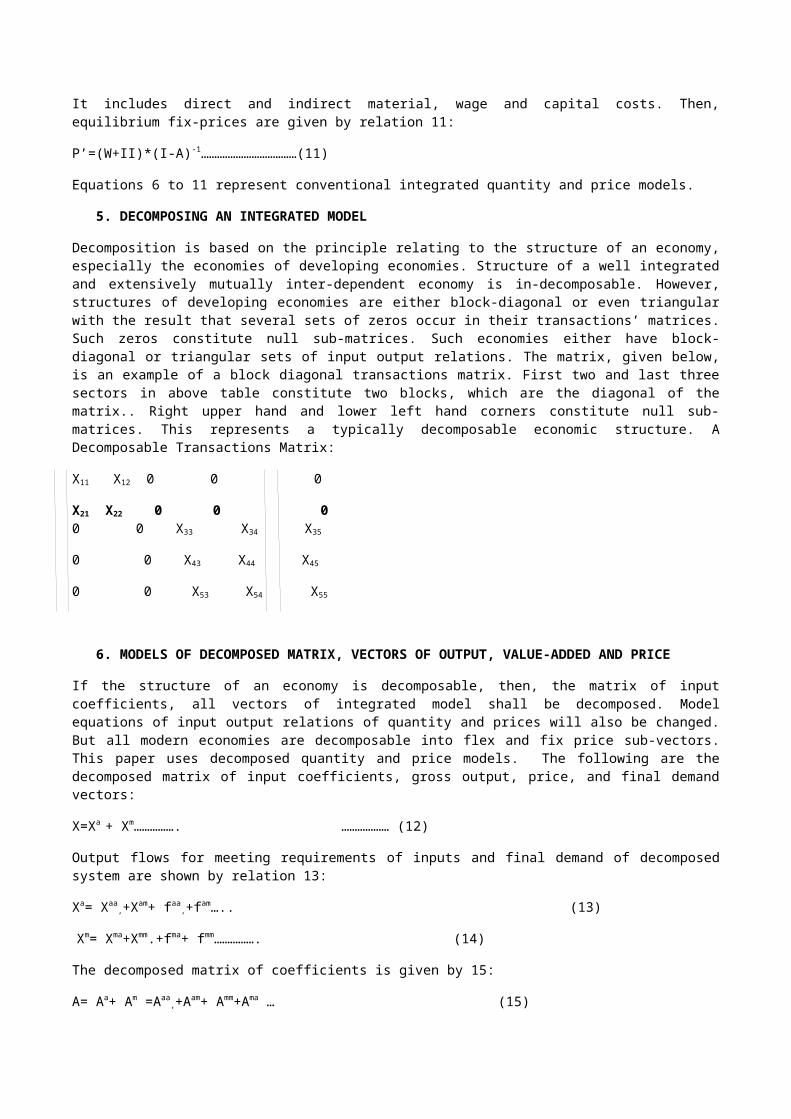
Decomposition is based on the principle relating to the structure of an economy, especially the economies of developing economies. Structure of a well integrated and extensively mutually inter-dependent economy is in-decomposable. However, structures of developing economies are either block-diagonal or even triangular with the result that several sets of zeros occur in their transactions’ matrices. Such zeros constitute null sub-matrices. Such economies either have block-diagonal or triangular sets of input output relations. The matrix, given below, is an example of a block diagonal transactions matrix. First two and last three sectors in above table constitute two blocks, which are the diagonal of the matrix.. Right upper hand and lower left hand corners constitute null sub-matrices. This represents a typically decomposable economic structure. A Decomposable Transactions Matrix:

X11 X12 0 0 0

X21 X22 0 0 0 0 0 X33 X34 X35

0 0 X43 X44 X45

0 0 X53 X54 X55

6. MODELS OF DECOMPOSED MATRIX, VECTORS OF OUTPUT, VALUE-ADDED AND PRICE

If the structure of an economy is decomposable, then, the matrix of input coefficients, all vectors of integrated model shall be decomposed. Model equations of input output relations of quantity and prices will also be changed. But all modern economies are decomposable into flex and fix price sub-vectors. This paper uses decomposed quantity and price models. The following are the decomposed matrix of input coefficients, gross output, price, and final demand vectors:

X=Xa + Xm……………. ……………… (12)

Output flows for meeting requirements of inputs and final demand of decomposed system are shown by relation 13:

Xa= Xaa,+Xam+ faa

,+fam….. (13)

Xm= Xma+Xmm.+fma+ fmm……………. (14)

The decomposed matrix of coefficients is given by 15:

A= Aa+ Am =Aaa,+Aam+ Amm+Ama … (15)

Aa=Aaa,+Aam……………………… (16)

Am =Amm+Ama……………………… (17)

The following are the decomposed final demand value added vectors:

f= fa+fm=faa,+fam+ fma+ fmm………. (18)

V=Va+Vm=Vaa+ Vam+Vma+ Vmm (19)

Conventional price vector of equation 7/11 is also split into two parts of Flex and Fix Prices:

P’= Pa’+ Pm’…………………………………. (20)

Where Pm’t =Vector of Fix-prices, and Pa’

t= Vector of Flex-prices at time t. The conventional price model is now given by relation 21:

P’=MC =MV*(I-A)-1……………. (21)

M=(1+λ)………………………… (22)

Vector of scalars, λ comprises mark-up-rates over long run cost of production, C, of different sectors. Different rates of mark-up apply to the long run cost of production of different sectors to determine prices. Mark-up rate λ j of sector j, j=1,2,….130 is determined as follows:

λj={ Pj-Cj}/Cj…………………… (23),

j=1,2,…130. Relations 11 and 23 together yield the price relation 24:

P’={1+ λ)C={1+ λ)(W+II)*(I-A)-1………. (24)

Equation 24 still represents the conventional integrated price model, which needs decomposition for distinguishing flex from fix prices. This needs bifurcation of the scalar λ into λm and λa;

λm≤ 0.20∧¿ λa¿0.20 . Mark−¿up rate may also be expressed in percentage terms.&&&&&

DECOMPOSED MODELS OF FIX AND FLEX PRICES

The above decomposition of price vector into two sub-vectors of flex and fix prices furnish two price models 1:

Pm= M1Cm…………………… (25)

M1={1+ λm}…………………………. (26)

The scalar λm<0.20 is defined as earlier, but M1<1.20 and M2¿1.20 and λa>0.20. If s is the total number of flex price sectors, then, a=1,2,….s and m=s+1…..130 Substituting M1 from 26 into 25 yields relation 27:

Pm={1+ λm}Cm ………._ (27)

M2 refers to flex prices Long run average cost of production of all fix price sectors is assumed to be determined by relation 28. Reason is obvious. Technology of production of flex price sectors does differ from the technology used in fix price sectors; the technological differences are captured by the decomposed parts of matrix A.

Cmt= (1+ λm )P’m

tAmm +(1+ λa)P’ta Aam+Vm

t……………… (28)

Substituting value of Cmt from equation 28 in equation 27 yields equation 29:

P’mt ={1+ λm){P’m

t Amm +(1+ λa )(P’at Aam+Vm

t}……………… (29)

Re-organization of terms of equation 29 yields relation 30:

P’mt –(1+ λm) P’m

tAmm)= {(1+ λa) P’at Aam+Vm

t}

P’mt{I-Amm(1+ λm)}= {(1+ λa) P’a

t Aam+Vmt}

P’mt= {(1+ λa) P’a

t Aam+Vmt}{(I-Amm) -1 (1+ λm)]……… (30)

7. APPROPIRATENESS OF INPUT OUTPUT MODELING OF INFLATION

Empirical exercises are based on two basic models: (1) S. Prakash’s Flex-Fix Price Model (1981), and (2) Decomposition Models, which are an extension and modification of basic Prakash model. Initial two models of preliminary exercise used for the identification of flex and fix price sectors are not used at this stage. These two models have served the purpose for which these were formulated. The table 2, given below, show all six models .

TABLE:1- MODELS USED TO DETERMINE CONVERGENCE OF DEMAND PULL TO COST PUSH

MODELS

These six models are developed from the two model equations of flex and fix price systems. Decomposition models are modified and extended versions of flex and fix price models. Decomposition of basic model is an innovation used in this paper. Two models of Flex and Fix price systems (Equations) and Decomposition Models and the procedures followed in the application of these six models are elaborately explained here-under.

QUANTITY AND PRICE MODS

Like the Linear Programming Modeling, Input Output modeling also has two models- Primal and it’s Dual. Quantity model is defined as primal and price model is defined as its dual. Both, these aSLeontief’s primary models are outlined hereunder:

Source:Authors” own construction

Upper part of the decomposed models comprises all 130 sectors, which receive inputs only from flex-

Decomposed model comprises 4 parts: One upper part and one lower part.. Each part has two components.: First segment comprises only 27/41 flex-price sectors and represents the square sub-,matrix: flex-price *flex-price sectors. The second segment of this upper part of the matrix comprises the sub=matrix of 27/41 flex* 103/89 fix price sectors. All sectors of these two segments of sub-matrices receive inputs only from flex-price sectors. Thus, the decomposition model classifies the upper segment of flex-price system into two sub-matrices: (27x27)/ (41x41) of flex to flex and (27x103)/(41x89) of

flex to fix price sectors. In these two sub-components, all inputs are received from flex price sectors; these inputs are used in the production of flex-price sectors themselves in the first segment; only flex-price inputs are used in the production of fix-price goods contained in second component. Both these segments together capture the dependence of both flex and fix-price sectors on flex prices sectors.

Similarly, lower part of the original matrix, A is decomposed into two segments: first segment (third of the overall matrix) depicts the supplies of fix-price intermediate inputs to meet the demand of flex-price sectors for fix-price inputs. This segment depicts the dependence of flex on fix-price sectors for the supply of requisite inputs of fix-price goods: (103x27)/(89x41). Other corresponding (fourth) component of the lower segment of the original matrix represents (103x103)/(89x89) fix price sectors’ dependence on each other. Thus, the lower segment of the original matrix has 103/89 fix-price sectors which supply inputs of fix-price goods for use in the production of 27/41 flex price sectors and 103/89 fix-price sectors. Modification of model equations 7 and 9 is based on the above decomposition of the original transactions/coefficients matrices into four parts. Decomposition models are modified and extended versions of flex and fix price models. Decomposition of basic model is an innovation used in this paper. Two models of Flex and Fix price systems (Equations) and Decomposition Models and the procedures followed in the application of these models are elaborately explained here-under.

8. IDENTIFICATION OF FLEX PRICE SECTORS

Model equation 11 is applied to estimate equilibrium prices of 130 sectors of Indian economy, which are used as the bench mark for separating sectors of fix and flex prices. Table 1 in contains the list of 41 flex price sectors. M2 >1.20, forall j=1,2,…, 41, if 20% is accepted as the mark-up rate over long run cost of production. This mark up rate is based on the findings of studies of Anita (1986) and Keya Sengupta (1992) and the company data of Prowess. Prowess furnishes detailed accounts of more than 20,000 companies of Indian economy. Flex price sectors are numbered from 1 to 41. M j≤1.20 for all j=42, 43, …,130, if all fix price sectors are numbered from 42 to 130. Thus, the composite price vector comprises 41 flex and 89 fix prices. These 41 flex price sectors are listed in table 1 given below.

TABLE 2: LIST OF 41 FLEX-PRICE SECTORS

1 2 3 4 5 6 7 8 9 10 11

Paddy Wheat Jowar Bajra

Maize Gram Pulses

Sugarcane

Groundnut

Coconut Other oilseeds

12 13 14 15 16 17 18 19 20 21 22

Jute Cotton Tea Coffee

Rubber

Tobacco Fruits

Vegetables

Other crops

Milk and milk products

Animal services(agricultural)

23 24 25 26 27 28 29 30 31 32 33

Poultr

y & Eggs

Other liv.st. prod

u. & Gob

ar Gas

Forestry and

logging

Fishing

Coal and

lignite

Natural gas

Crude petroleum Iron ore

Manganese ore

Bauxite Copper ore

34 35 36 37 38 39 40 41

Other metall

ic

Lime ston

e Mica

Other non

metall Sugar

Khandsari,

boora

Hydrogenated

oil(vanasp

Edible oils

other

miner

als

ic miner

als ati)

than vanaspa

ti Source: Based on Authors’ calculations and exercise of identification

9. RESULTS OF EMPIRICAL ANALYSIS OF I-O PRICE MODELS

Flex prices alone are allowed to change initially in application of models developed in the paper. This artifice facilitates isolation of the effect of change in flex prices on the Indian price system.. If this has not been done, impact and effect of changes of flex prices along with changes in fix prices would have been intermingled. It would have made it difficult to separate the effect of change in flex on fix prices from the effect of change in fix prices on themselves. Besides, effects of mutual actions and interactions of two sets of prices would have also been mixed. It would have made it difficult to verify and validate the postulation that the demand pull converges towards cost push inflation in Indian economy.

The separation of mutual effects of flex and fix prices is also warranted by two facets of theoretical thrust of the paper: (i) Inflation emanates from flex price sectors, especially food grains and other important crops in Indian economy. There from it spreads to the rest of the economy; and (ii) The Modeling approach facilitates evaluation of second preposition of the paper that once demand pull inflation has emerged in the Indian economy from agriculture and other flex-price sectors, it converges towards cost push inflation. Subsequently, cost push inflation also begins accentuating inflationary spiral across all sectors of the economy further. Once the rising food prices have engulfed the economy in its trap, wage hikes, increased interest rate and escalation of economic value added follow in its trail. Percolation of inflation from one to other sectors and the underlying argument in above postulates may be illustrated by the graph-1 given below:

Flow Graph-1 Convergence of Demand Pull into Cost Push Inflation

Source: Authors; own construction

10. DEMAND PULL AND SENSITIVITY ANALYSIS

FLEX PRICE SECTORS (27/41Sectors)

(DEMAND PULL

ECONOMIC VALUE ADDED

WAGE INTEREST

IncreaseFIX- PRICE SECTORS

(103/89 Sectors)(

Increase

Value Added= Wages + Interest Profits/ EVA

VA = W + R + EVA

Sensitivity analysis is based on the results of two exercises which explore responses of both flex and fix–price sectors to changes of 5%, 10%, 15% in flex prices of 27/41 sectors. These changes in flex prices first affect all flex price sectors directly and indirectly. But these changes in flex prices also affect prices of such sectors as agro-based and agro linked industries and other industries, which use flex-price inputs in production. Prices of sectors, which do not use flex price inputs in production, are affected only indirectly. Indirect effects flow from increase in wage and interest rates and general inflationary expectations.

Degree of responsiveness of flex prices to initial shortfall in supply and the subsequent rates of change in prices are defined as Demand Pull Inflation in so far as the existing demand for agricultural goods exceeds reduced supply of crop outputs in years of scanty rainfall. Initial demand pull inflation is accentuated by being fed on inflationary expectations of intermediate traders.

Demand pull inflation tends to be cumulative in subsequent rounds. As total cultivable area is, more or less fixed during cultivation seasons, if more area is put under one crop, it leaves less area for other crops. Crop outputs also become fixed after harvesting. But crop outputs commanding currently higher relative prices, are allocated more area in subsequent season which reduces supplies of such crops in next season. Consequently, prices of such crop outputs rise in subsequent seasons (See, Prakash, Buraghain and Sharma, 1992). Above discussion highlights that demand pull inflation feeds on its own steam and it affects general price level directly as well as indirectly through backward and forward linkages.

11. DIVERSITY OF FIX-PRICE SECTORS

Fix-price sectors are highly diversified.. These sectors are (i). Agro based industries1; (ii). Agro linked industries2; (iii). Heavy and basic goods industries; (iv) Machinery and Equipment industries; (v) Light durable consumer goods industries, etc; (vi) Energy Sectors; (vii) Packaging Materials and Basic Chemicals, (viii) Infrastructure sectors; and (ix) Public administration, Financial and other services. Therefore, margins over average costs differ significantly among these sectors..

First two groups of fix price industries bear the direct and indirect effects of changes in flex prices. But such fix price sectors as heavy and basic goods industries and durable consumer goods industries bear mostly indirect effects of changes in flex prices. Inflationary pressures of direct and indirect effects of linkages of flex with fix-price sectors also lead to (i) wage hikes for protecting real wages and salaries. Central and state governments, public enterprises etc. grant additional DA to neutralize inflation effect on real wages, it rises nominal wage and salary rates; (ii) higher interest cost due to high interest rate policy, and (iii) increase in economic value added components of value added vector also accentuate inflation effect of flex prices..

This paper uses linkages between flex and fix price sectors of modern economies, where prices are determined on different principles. Consequently, flex and fix prices behave differently. These prices move through different routes of inflationary process. The divergence between flex-fix price markets warrants different approach to the analysis of inflation. Hence, this paper diverges from conventional wisdom and uses structural rather than monetary approach.

12. PROCEDURE OF SEPARATING FLEX-FIX PRICE SECTORS EMPIRICALY

130x130 matrix, A is split into four parts as follows:

Aaa=(27x27)/(41x41); Aam=(27x103)/(41/89); Ama=(103x27)/89/41); Amm= (103x103)/(89x89).

The transaction matrix is used as the base for this purpose. Leontief’s inverse of Aaa and Amm are estimated as per usual procedure from square transactions/coefficients matrices, which are adjusted by specified rates of change of flex prices in empirical exercises. Inversion of square first and fourth sub-input coefficients matrices is possible. For deriving Leontief inverse of Aam and Ama, the non-square sub-matrices of decomposed A-matrix are augmented to make these squares. Null matrix of 77x103 is added to Aam and a null matrix of 103x77 is added to Ama. Original vector of value added of 27/41 sectors is proportionately decomposed into two parts according to the ratios of two sets of intermediate inputs of these components.. Initial value added vector of 130 sectors is decomposed proportionately into sub-components of fix price sectors. This distribution is based on I-O model’s basic assumption of constant returns to scale and fixity of input coefficients. Consequently, monetary value of output increases proportionately in response to increases in the values of inputs resulting due to increase in cost of flex price inputs This yields four value added sub-vectors corresponding to four-fold decomposition of coefficients matrix: Vaa

, Vam, Vma, Vmm. Value added vectors Vam, and Vma are also augmented by additions of requisite number of zeros. This is done to match the second and third components of output vector and technology matrices and their corresponding inverses. Inverses of these four decomposed matrices and value added vectors are used for determining 4 sets of prices.

Equation 2 furnishes an estimate of cost based prices on the assumption that all sectors are fix-price sectors. First 27 sectors are identified as flex-price sectors on a priori reasoning and empirical evidence furnished by earlier studies. Flex-prices are determined by demand, which is governed generally by inflationary expectations and stocking behavior of independent intermediate traders and public agencies. MSP is also determined on the principle of cost plus pricing and 15-19% mark up on cost is generally used in the fixing fix-prices. Thus, fix-prices are determined on cost plus 15-20% basis (Cf.Oxford Economists Group, Also See, Anita, 1985).

Cost based prices of 130 sectors are calculated as a first step. This furnishes the base for comparison. The cost–based prices of the model are compared with the observed procurement prices that prevailed in the regulated mandis of India in 2008. It is observed that stiff competition prevails in agricultural markets for the procurement of food-grains and other essential commodities between public agencies, whole sale dealers, agents of mill owners and public agencies. The competition makes procurement prices ultimately converge to market prices in all seasons of the year irrespective of bumper or scanty harvests. Competition between the government and private agents is intense during the years of scarce supplies due to output being below normal. During such periods, state governments also announce incentives to further enhance MSP to encourage farmers to sell output to government agencies. This step is essential to check inflation and maintenance of public stock at the desirable level. Off take from public distribution system increases during such years,. However, the fierce bidding up of prices in the grain markets adds to the inflationary spiral in the economy. This results in blowing up the flex prices above the earlier level.

The value added vector of 103 fix-price sectors is increased by 15%. Margins/mark-ups over the calculated bench mark costs are used for determining the base fix-prices. This furnishes estimates of cost based prices of all 130 sectors of the economy; these are defined as Base Prices.

Base prices are used for simulating responses of both flex and fix-prices to 5%, 10% and 15% and 23% increase in flex-priced inputs of sub-sets/components one and three of decomposed model equations, 11 and 30.. Model equations 11 and 30 are used to determine the responses of fix-prices to the specified changes in flex-prices.

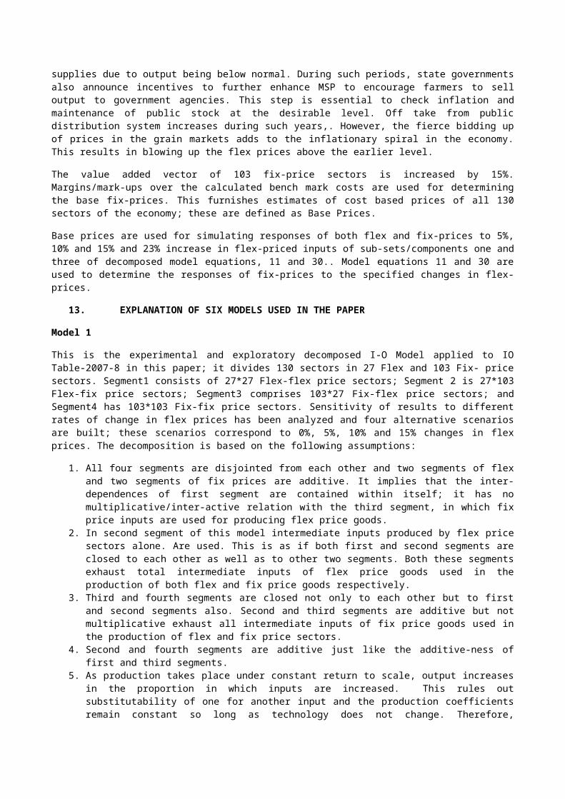
13. EXPLANATION OF SIX MODELS USED IN THE PAPER

Model 1

This is the experimental and exploratory decomposed I-O Model applied to IO Table-2007-8 in this paper; it divides 130 sectors in 27 Flex and 103 Fix- price sectors. Segment1 consists of 27*27 Flex-flex price sectors; Segment 2 is 27*103 Flex-fix price sectors; Segment3 comprises 103*27 Fix-flex price sectors; and Segment4 has 103*103 Fix-fix price sectors. Sensitivity of results to different rates of change in flex prices has been analyzed and four alternative scenarios are built; these scenarios correspond to 0%, 5%, 10% and 15% changes in flex prices. The decomposition is based on the following assumptions:

1. All four segments are disjointed from each other and two segments of flex and two segments of fix prices are additive. It implies that the inter-dependences of first segment are contained within itself; it has no multiplicative/inter-active relation with the third segment, in which fix price inputs are used for producing flex price goods.

2. In second segment of this model intermediate inputs produced by flex price sectors alone. Are used. This is as if both first and second segments are closed to each other as well as to other two segments. Both these segments exhaust total intermediate inputs of flex price goods used in the production of both flex and fix price goods respectively.

3. Third and fourth segments are closed not only to each other but to first and second segments also. Second and third segments are additive but not multiplicative exhaust all intermediate inputs of fix price goods used in the production of flex and fix price sectors.

4. Second and fourth segments are additive just like the additive-ness of first and third segments.5. As production takes place under constant return to scale, output increases in the proportion in which inputs are

increased. This rules out substitutability of one for another input and the production coefficients remain constant so long as technology does not change. Therefore, segmentation of transaction matrix does not influence these properties of I-O model.

6. The cost of inputs of a particular good is increased by the same margin by which its price and value of output increases.

7. As the value of output and inputs of a commodity rise together, value added has also to rise for two reasons. Firstly, only a small fraction of output of a commodity is used as an input in production of any other commodity and its impact is thinned out in the input coefficeints of producer sectors. Therefore, value added of a sector is assumed to increase by the proportion equal to the average increase in value of sum of inputs; this assumption is warranted to maintain constant returns to scale. Secondly, under inflationary pressures, wage and interest cost

and profit/ economic value added also increase. On the basis of the findings of past researches, sum of these components of value added is increased by 50% while value added vectors of second and fourth segments are increased by 15%.

(Note: For steps followed in the application of above model, see appendix 1)

Model 2

This is also an experimental and exploratory exercise which uses cost based price model of Prakash, S. (1981). This model also divides 130 sectors into two markets i.e. Flex and Fix price markets. Flex price markets comprise 27 sectors and fix price markets have 103 sectors. Sensitivity of results to different rates of change in flex prices has been analyzed and four alternative scenarios are built on the basis of 0%, 5%, 10% and 15% increase in flex prices.

(Note: For steps followed in the application of this model, see appendix)

Model 3

This is also an extended, experimental and exploratory decomposed I-O Model; but this model is applied to 41 flex and 89 fix price sectors. Reason is that 14 out of 103 sectors are transferred from fix to flex price category. But sensitivity analysis is carried out on the four alternative scenarios built on the basis of introduction of 0%, 5%, 10% and 15% increase in flex price inputs in this case also.

RATIONALE OF INCREASING FLEX PRICE SECTORS

The Results of experimental models 1 and 2 highlighted differential levels of responses of prices of different sectors of both flex and fix price groups. Fourteen out of 103 sectors, identified as fix price sectors in first exercise, are found to be most responsive to all 4 rates of change in flex price inputs as these sectors are heavily dependent on the use of flex price inputs in their production.

Four new decomposed segments now are as follows:

Segment-1: 41*41; Segment-2: 41*89; Segment-3: 89*41; Segment 4: 89*89. But all other arguments do not change.

(Note: Steps followed in this model see in appendix)

Model 4

This is also an extended, experimental decomposed model constructed on the basis of Prakash, S. model (1981).

This model also reclassifies 130 sectors of Indian economy into two markets i.e. Flex and Fix price markets. Flex price markets comprise 41 sectors and fix markets have 89 sectors. Sensitivity of results derived by the application of the same 4 different rates of increase in flex prices has been analyzed on the basis of four alternative scenarios built by implementing 0%, 5%, 10% and 15% increase in the prices of flex price inputs as has been done in earlier exercises.

(Note: Steps in application of this model are reported in appendix)

Model 5

Observed increase in retail prices of 41 sectors are used to raise the cost of flex price inputs used in production processes in four decomposed segments of Indian economy.

(Note: Steps to be followed in this model see in appendix)

Model 6

This model is not based on decomposition of the system in four parts; it rather determines flex and fix prices on the basis of model equation 1 of fix prices and model equation 2 of flex prices. The model has used real increase in retail prices of 41 sectors rather than 5, 10 and 15% rise. Real increase in prices of flex price inputs is used to adjust transaction matrix

(Note: Steps followed in this model are explained in appendix)

14. ANALYSIS OF EMPIRICAL RESULTS

Empirical results are analyzed sequentially model wise. A two -fold comparison is made between average change in prices evoked by the given percentage increase/decrease in flex prices; and secondly, comparison is made with prices observed without change in flex prices. Additional comparison is made between the maximum and minimum responses of flex and fix prices to the given percentage changes in the costs of flex priced inputs. The results of calculations are reported in appendix table.

15. DISCUSSION OF RESULTS OF MODEL-3

The table reveals that flex prices have changed, on an average, by 5.17% in response to 5% increase in flex priced inputs; 9.75% change is shown in flex prices in response to 10% change and 15.38 % change is recorded in response to 15% change in flex priced inputs. The pattern of these changes indicates an oscillating response of flex prices to changes in costs of flex priced inputs. The degree of response of flex prices oscillates with oscillations of causative changes in prices of flex priced inputs. But the percentage of changes in response to changes in costs of flex priced inputs either matches the given percentage change in costs of flex priced inputs approximately, or it exceeds the given change marginally or more. Consequently, average elasticity of flex prices with respect to changes in costs of their own inputs, on an average, is 1.01. The flex prices are thus elastic with respect to the changes in the costs of flex-priced inputs. In fact, the rate of change in flex prices is 1% more than the rate of change in the cost of flex price inputs. It may, therefore, be inferred that the demand pull inflation tends to be accentuated by its own steam but the rate of accentuation is slightly greater than the initial change in the cost of flex price inputs. A 100% initial increase in cost of flex priced inputs results in 101% change in flex prices. Thus, demand pull inflation is self feeding. Besides, these results also lend credence to the authors’ postulation that inflation in Indian economy emanates from flex price sectors. Flex prices generally increase in response to the shortfall in supply relative to demand, especially agricultural goods.

Fix prices as against flex prices, respond, on an average, relatively mildly to the given changes in flex prices. The fix prices change less than proportionately to 5, 10 and 15 percent changes in costs of flex priced inputs. Actual responses of fix prices, on an average, to 5, 10 and 15 percent changes in costs of flex price inputs are 2.70, 8.11 and 9.29. Thus the increase in fix prices evoked by increase in costs of flex price inputs generally tends to be lower than the increase in cost of flex priced inputs. Consequently, elasticity of fix prices with respect to flex prices is only 0.57. Thus, the fix prices are much less elastic to the changes in the changes in flex prices than the flex prices themselves. But an average change of 57% in fix prices in response to changes in flex price system cannot be overlooked as measly. Response of fix prices to given changes in flex prices is muted by the presence of a large number of sectors in fix price group, which are only indirectly affected by changes in flex prices. There are only 17 out of 103 fix price sectors, which either draw their inputs from flex price sectors, or supply their output for use as inputs in the production processes of flex price sectors. Actually, 86 sectors are only indirectly related to flex price sectors. Therefore, these sectors absorb only indirect impact of change in flex prices. A part of the impact of change in flex prices emerges as the increase in production costs of wages and interest and increase in EVA; these three factors also cause fix prices to rise in response to changes in flex prices. On the whole, both sets of these results lend credible evidence to support the author’s twin hypotheses that (i) inflation emerges from flex price sectors, and (ii) demand pull inflation, generated by flex price sectors, converges to cost push inflation.

16. COMPARISON OF TOP TEN SECTORS OF FLEX AND FIX PRICES

It is observed that different sectors respond differently to any given rate of increase in prices of flex prices. Therefore, the response rates of top most sensitive sectors to the changes in the flex prices are compared. The results of calculations are reported in the table given below. Responses rates of top 10 flex price sectors with respect to increase in flex prices at the specific rates are similar quantitatively. Most of these sectors maintain their respective ranks irrespective of the changes in rates of change in flex prices due to constancy of technology. Observed individual and average responses to changes in flex prices exceed the initial change. But as the rate of change in flex prices increases, response rates of fix prices change more than proportionately. Consequently, average of elasticity of elasticity with respect to three rates of change in flex prices remain stable at 1.41- 1.42. Thus, on an average, prices of top ten fix price sectors show an increase of 141-142% to an average increase of 100% in flex prices. Thus these top ten fix price sectors sensitive to change in flex prices are highly elastic.

Among these top 10 sectors, minimum response to 5% change in flex prices is 6.26% in fishing, whereas maximum response of 8.11% is for animal services sector. The response rates of other sectors to these three rates of change in flex prices hover approximately around 7%. Rates of 10% and 15% increase in flex prices also evoke minimum and maximum responses from fishing and animal services sectors.

More detailed picture is shown by the table 2.

Table 3: Top 10-Flex Price Sectors of Model-3 at 5,10 and 15%

Rank Sectors 5% Sectors 10% Sectors 15%1 Animal Services 8.11 Animal Services 16 Animal Services 24.42 Hydrogenated oil 7.7 Hydrogenated oil 15.12 Hydrogenated oil 23.063 Bauxite 7.46 Khandsari 14.29 Khandsari 22.424 Khandsari 7.22 Bauxite 14.19 Bauxite 21.735 Sugar 7.14 Sugar 14.14 Sugar 21.516 Edible oils 7.01 Fruits 14.07 Fruits 21.377 Fruits 6.98 Edible oils 13.76 Edible oils 20.978 Vegetables 6.49 Vegetables 13.04 Vegetables 19.73

9 Other liv. St. product. 6.44Other liv. St. product. 12.8 Other liv. St. product. 19.39

10 Fishing 6.26 Fishing 12.03 Fishing 19.24

COMPARISON OF BOTTOM TEN SECTORS OF FLEX AND FIX PRICES

Results are reported in the table below. A perusal of the table 4 reveals that

(i) Responses of flex prices of bottom ten sectors to any given rate of change in flex price inputs used in production differ between the sectors quite a bit;

(ii) Responses of flex price bottom ten sectors to the different rates of change in costs of flex priced inputs also differ between these ten sectors and between the rates of change in flex prices;

(iii) Responses of flex prices of bottom ten sectors to differential rates of change in the costs of flex priced inputs tend to increase with rate of increase in the costs.

(iv) The same ten flex price sectors occur among the bottom ten sectors in all three cases of increased cost of flexed priced inputs. However, their ranks tend to change with a change in rate of increase in costs.

(v) Average elasticity of all bottom ten flex price sectors with respect to average of three rates of change in flex priced inputs is as high as 0.51. This elasticity is comparable with the elasticity of top ten fix price sectors. Thus even the bottom ten flex price sectors are slightly more elastic than ten top fix price sectors with respect to change in flex priced inputs used in production.

Table 4: Bottom 10-Flex Price Sectors of Model-3 at 5,10 and 15%

Rank Sectors 5% Sectors

10% Sectors 15%

1 Other Non metals 3.88 Rubber 6.4 Natural Gas10.9

82 Natural Gas 3.87 Natural Gas 6.2 Other Non Metal 10.6

3 Mica 3.79 Other Non Metal5.2

9 Rubber10.0

4

4 Coal and Lignite 3.63 Coal and Lignite5.2

1 Coal and Lignite10.0

1

5 Rubber 3.26Crude and Petroleum

5.13 Mica 9.75

6Crude and Petroleum 3.23 Mica 4.6

Crude and Petroleum 9.03

7 Iron Ore 2.6 Lime Stone 2.7 Iron ore 6.53

8 Lime Stone 2.52 Iron Ore2.6

7 Lime Stone 6.41

9 Copper ore 2.26 Copper Ore2.1

3 Copper ore 5.79

10 Magnese Ore 0.97 Magnese Ore0.4

1 Magnese ore 2.31

Table 5: Bottom 10-Fix Price Sectors of Model-3 at 5,10 and 15%

Rank Sectors 5% Sectors

10% Sectors 15%

1Wood and Wood Products 1.3 Tea and Coffee

7.81 Beverages 5.69

2 Jute, Mesta Textiles 0.96 Fertilizers7.7

7 Cotton Textiles 5.5

3 Beverages 0.89 Cotton Textiles7.7

2Non ferrous Basic Metals 5.44

4 Tea and Coffee 0.68 Other Chemicals7.6

8 Jute, Mesta Textiles 4.97

5 Cotton Textiles 0.57Non ferrous Basic Metals

7.65 Other Chemicals 4.42

6 Other Chemicals 0.52 Beverages7.4

9Wood and Wood Products 4.24

7 Petroleum Products 0.51Hostels and Restaurants

7.29 Petroleum Products 3.24

8 Coal Tar Products 0.38 Mis. Prodcuts6.7

7Hostels and Restaurants 2.89

9 Mis. Prodcuts-

1.24 Coal Tar Products6.4

9 Coal Tar Products 2.32

10Hostels and Restaurants

-0.74

Petroleum Products

2.93 Mis. Prodcuts 2.07

So far as the response of bottom ten fix price sectors to the average of three specific rates of change in the cost of flex priced inputs is concerned, the average elasticity is 0.38. This is much lower than the corresponding elasticity of bottom ten flex price sectors.

17. DISCUSSION OF RESULTS OF MODEL 4

This model focuses on the results of two equations one of which exclusively deals with the determination of 41 flex prices as an addition of inputs’ costs of both flex and fix priced inputs used in production of these flex price sectors. Second equation of this model deals with the determination of fix prices of 89 sectors which is a sum of effect of both flex and fix priced inputs used in their production. Results are reported in table given below.

The average increase in costs of flex priced inputs as in earlier model still remains 10%. The results reveal that the response rates of 41 flex price sectors to 5, 10, 15% changes in the costs of flex priced inputs used in production differs among the flex price sectors as well as fix price sectors. The rates of change in flex prices of 41 sectors in response to 5, 10 and 15% change in the cost of flex priced inputs are 6.60, 13.19 and 19.78. This shows that the changes in flex prices of 41 sectors are much greater than the corresponding changes in the costs. These twin rates of change in flex prices and their costs imply much greater than unit elasticity of flex prices. As against the flex price sectors, 89 fix price sectors show 8.49, 16.73 and 24.71% changes in fix prices when the prices of flex priced inputs increase by 5, 10 and 15%. These changes also imply greater than unit elasticity for 89 fix price sectors with respect to changes in flex prices.

Table 6: Top 10-Flex Price & Fix Price Sectors of Model-4 at 5, 10 and 15%

Rank Flex Sectors 5% 10% 15% Fix- Sectors 5% 10% 15%

1 Bauxite11.9

923.9

735.9

6

Legal Services and Renting of Machinery 9.97

19.93

29.88

2 Animal Services9.92

719.8

529.7

8Ownership and dwellings 9.95

19.90

29.84

3 Hydrogenated oil8.55

617.1

125.6

7 Banking 9.8819.7

429.5

74 Khandsaari 8.42 16.8 25.2 Education and 9.88 19.7 29.5

5 5 8 Research 3 6

5 Sugar8.30

616.6

124.9

2 Other Services 9.8519.6

729.4

6

6 Mica8.18

215.8

123.4

4O.com, social &personal services 9.83

19.63

29.41

7 Edible oils7.68

615.3

723.0

6Computer and Related Activities 9.83

19.63

29.40

8Other Mettalic minerals

7.417

14.83 21.6 Real Estate Activities 9.82

19.62

29.35

9 Coffee 7.2614.5

221.7

8 Trade 9.8119.5

929.3

3

10 Crude Petroleum7.19

9 14.4 21.6 Communication 9.80

419.5

729.3

1

Among the top 10 flex and fix-price sectors, ranks of individual flex price sectors do not vary with the rates of change in flex prices. Thus, the top ten flex price sectors display stability in their response rates to variations in the flex price input costs. The average elasticity of top ten flex price sectors with respect to average 10% increase in flex priced inputs is 1.69. Thus, one percent increase in costs of flex price inputs causes flex prices of top ten sectors to increase by as much as 1.69%. All these sectors are highly elastic with respect to the flex prices. This aso shows that the elasticity of top ten flex price sectors is much greater than the corresponding elasticity of top ten flex price sectors of model 3. This difference is caused by the loss of information due to decomposition and greater interaction effect of both groups of sectors being considered as additives.

As against the flex price sectors, the elasticity of the top ten fix price sectors is as high as 1.97. Therefore, 1% change in the costs of flex priced inputs make top ten fix prices change by as much as 1.97 per cent. Obviously, top ten fix price sectors are much more elastic with respect to the change in the costs of flex priced inputs.

Interestingly, the top ten highly elastic flex price sectors comprise agriculture and auction based mining products, which consistently respond highly to changes in flex prices, irrespective of rates of change.

Table 7: Bottom 10-Flex Price & Fix Price Sectors of Model-4 at 5,10 and 15%

Rank Flex Sectors 5% 10% 15% Fix- Sectors 5% 10% 15%

1Milk and Milk Products

5.579

11.16 16.74 Beverages

7.468

14.48

21.04

2Forestry and Logging 5.55 11.1 16.65

Non Ferrous Basic Metals

7.362

14.24

20.65

3 Tea 5.4810.9

6 16.44 Cotton Textiles 7.2914.0

920.3

9

4 Groundnut5.38

610.7

7 16.16 Fertilizers7.11

4 13.719.7

7

5 Pollutry and Eggs5.37

210.7

4 16.11 Other Chemicals6.89

913.2

419.0

1

6 Cotton5.29

610.5

9 15.89Hotels and Restaurants 6.36

12.11

17.26

7 Sugarcane 5.2810.5

6 15.84Tea and coffee processing

6.199

11.71

16.53

8 Vegetables5.24

710.4

9 15.74 Coal Tar Products4.71

5 8.4711.2

7

9 Tobacco5.21

310.4

3 15.64 Misc. food Products3.87

8 6.7 8.46

10 Fruits5.19

210.3

8 15.58 Petroleum Products0.24

8-

1.28-

4.57

The ranks of bottom ten flex and fix price sectors also do not vary with the variation in the flex prices. Average elasticity of bottom ten flex price sectors with respect to average rate of change in flex prices is 1.07 and the corresponding elasticity of bottom ten fix price sectors is `1.05. Thus, both flex and fix price bottom ten sectors are elastic to change in flex prices, though flex price sectors are more elastic than the bottom ten fix price sectors.

18. DISCUSSION OF RESULTS OF MODEL 5

This model deals with the repercussions of changes in observed flex prices in 2011-12. It is great deal difficult to obtain data of actual prices, though the time series of average inflation rates is accessible. But in case of implementation of input output model, one needs detailed commodity/sector wise data. Data relating to observed flex prices in 2012-13 became accessible a couple of days ago. These data shall also be used in future exercises.

This model also has 41 flex and 89 fix price sectors. Thus the dimensions of this model 3 are the same. This is also a decomposed model having four segments. Flex prices are, however, derived as the sum of prices of segments 1 and 3, while fix prices are derived as a sum of prices of second and fourth segments. The two constituent sums are calculated from the respective models of segments relevant to the sum. As usual, decomposition involves some loss of information. The results of ten top and bottom sectors of flex and fix price groups are reported in the table 8 given below.

Table 8: Top 10-Flex Price & Fix Price Sectors of Model-5

Rank Flex- SECTORS

Real Change FIX- SECTORS

Real Change

1 Pulses 87.64 Petroleum Products 42.642 Vegetables 24.71 Tobacco Products 25.133 Tea 19.2 Jute, hemp, mesta textiles 24.74

4 Tobacco 16.46Furniture and fixtures wooden 23.98

5 Wheat 12.14 Misc. Food products 23.62

6Hydrogenated oil 11.73 Wood and wood products 23.02

7 Sugar 10.14 Leather footwear 21.538 Fruits 7.68 Other Chemicals 21.14

9 Khandsaari 7.38Land tpt. Including via pipeline 20.98

10 Paddy 7.14 Air transport 20.31

Average change in observed flex prices is 23%; but some negative changes in flex prices are also included. This has affected the average adversely. But average elasticity of top ten flex price sectors is 0.89 and average elasticity of top 10 fix price sectors is 1.07. Top 10 fix price sectors are much more elastic to change in flex prices. Top three flex price sectors among the ten are pulses, vegetables and tea. All fix price sectors have registered an increase of at least 20%. But the minimum increase is 7%.

Table 9: Bottom 10-Flex Price & Fix Price Sectors of Model-5

Rank

Flex- SECTORS

Actual Change Fix- SECTORS

Real Change

1 Natural gas -16.66 Carpet weaving 16.52

2 Mica -18.42Iron steel & ferrous alloys 16.17

3 Bauxite -18.91 Education & Research 16.14 Jowar -22.82 Electricity 15.22

5Coal and Lignite -26.25

Inorganic and heavy chemicals 15.18

6 Copper Ore -31.32 Medical & health 14.747 Iron Ore -31.6 Tea & coffee processing 13.75

8Magnese Ore -37.64 Paper, paper products 10.36

9 Coffee -39.16 Hotels & Restaurants 8.02

10Crude Petroleum -39.26 Coal tar products 5.81

Bottom ten flex price sectors comprise jowar and coffee from agriculture and 8 sectors are of mining of auction markets. Bottom ten fix price sectors include mostly services. Average elasticity of bottom ten flex and fix price sectors with respect to change in flex prices is -1.23 and 0.57. Thus, these fix price sectors are relatively less elastic than flex price sectors with respect to changes in flex prices.

19. DISCUSSIOON OF RESULTS OF MODEL 6

This model moves away from decomposition mechanism; it comprises only flex and fix price sub-systems. Observed flex prices of 2011-12 and changes relative to prices of 2007-08, as in model 5, are used. Average change in observed flex prices in this year is 23%. Average change in flex prices resulting from observed average change of 23% in flex prices is 48%. The elasticity is 1.48. Thus, the flex prices are shown to be highly elastic with respect to the changes in flex prices themselves. In fact, 100% increase in flex prices results finally in an increase of 148%. But fix-prices increase by an average of 28%. The elasticity coefficient of fix-prices is 1.28. But the percentage change in fix prices is also much greater than 23% increase in the flex prices. An increase of 100% in flex prices results in an increase of 123% in fix-prices. Though the fix prices are less responsive to the changes in the flex prices than the flex prices, yet the fix prices are also highly elastic. These results highlight the impact of food inflation on Indian economy as a whole though money supply remains constant. This structural feature accounts for the ineffectiveness of high interest rate policy in India,

The tables given below report the response rates of top ten and bottom ten flex and fix price sectors to the given changes in the costs of flex priced inputs.

Table 10: Top 10-Flex Price and Fix Price Sectors of Model-6

Rank

Flex- SECTORS

Real Change FIX- SECTORS

Real Change

1 Jowar 82.56 Legal Services 45.57

2 Bauxite 74.166Renting of Mach. & Equipment 45.54

3 Bajra 58.11 Ownership of dwelling 45.49

4Animal Services 50.968 Real Estate Activities 44.67

5 Coffee 47.473 Education and Research 44.52

6Crude Petroleum 47.167

Computer and Related Activities 44.36

7 Copper Ore 36.7225 Banking 44.318 Mica 40.39 Other Services 43.91

9 Khandsaari 36.681O.com, social&personal services 43.707

10 Iron Ore 36.56 Communication 43.085

The above table shows that (i) top 10 flex price sectors have 4 agriculture and 6 auction market’s mining sectors. Most of the sectors in this list are those present in the results of model 5. The top ten fix price sectors of this model are also present in results of model 5; most of these sectors belong to services.

Change corresponding to 23% change in flex prices of these ten top sectors is as high as 51%, yielding as high value of the elasticity of these sectors as 2.232. Thus, 100% change in the flex priced inputs make top ten flex prices rise by as much as 232%. This is the greatest value of elasticity shown either by flex or fix price sectors for any of the 5 other models. The average change in top ten fix prices corresponding to 23% change in flex prices is 44.5% yielding as high value of elasticity as 1.94, which is substantially lower than that of flex prices. These results support the thesis that the high demand pull inflation observed in 2011-12 has resulted from an extremely high increase in prices of selected flex priced sectors. This has resulted not only in high cost push inflation but also in demand recession in fix- price sectors as a sequel to high flex-price based inflation. Results of this model also confirm the main hypotheses of the study that inflation in Indian economy originates from flex price sectors in general and agriculture in particular, but inflation does not remain confined to the sectors from which it arises. It envelops the entire economy in its grip over a period of time. Consequently what begins as demand pull ultimately ends up as cost push inflation in Indian economy.

Table 11: Bottom 10-Flex Price and Fix Price Sectors of Model-6

Rank Flex- SECTORS

Real Change FIX- SECTORS

Real Change

1Forestry and Fishing 26.58 Structural Clay Products 19.65

2 Sugarcane 26.39 Tea & Coffee Processing 18.993

3Milk and Milk Products 25.878 Electricity 17.596

4Other Non Mettalic 25.59

Non Ferrous Basic Metals 16.897

5 Tobacco 25.25 Other Chemicals 16.826 Tea 24.96 Misc. Food Products 10.446

7 Fruits 24.27Land tpt. Including via pipeline 9.66

8 Vegetables 23.715 Fertilizers 2.3619 Polutry and Eggs 15.46 Coal tar products -50.07

10 Pulses 10.44 Petroleum Products 184.8

Nine out of bottom ten flex price sectors are from agriculture, forestry, and animal husbandry. But the bottom ten fix-price sectors throw a highly mixed bag in this case. The percentage change in the flex prices remains 23% in this case also. But the corresponding average change in prices of bottom ten flex price sectors is 22.85%, furnishing 0.993 as elasticity. These bottom ten flex price sectors are just elastic with respect to the change in flex prices. This result differs from the results of bottom ten flex price sectors given by other 5 models.

But prices of the bottom ten fix-price sectors show an average increase of 24.71% which is slightly greater than 23% change in flex prices. So, the elasticity is 1.07. This shows that bottom ten fix price sectors are more elastic than bottom ten flex price sectors of this model. Thus, the results for bottom ten fix price sectors also differ from the results furnished by decomposed models. Loss of information involved in decomposition accounts for these differences between the results of model 6 and all other models used in practical applications in the paper.

20. OVERALL VIEW OF EMPIRICAL RESULTS

Results of model 1 and 2 are not analyzed in detail because (i) 27 flex and 103 fix price sectors are in the model 1; (ii) Second model is an integrated model, so it differs from model 1 which involves loss of information due to decomposition. Models four and six are also integrated models, the results of which are compared with those of decomposed models 3 and 5 respectively.

21. IMPACT OF CHANGE IN FLEX PRICES ON FLEX PRICES: DECOMPOSED MODEL 3 AND 5

The results of these models are compared in view of the following:

(i) Model 3, incorporates results of analysis of effect of 5, 10 and 15% changes in flex prices on flex and fix price systems. These changes are hypothetical. They constituent a part of the exercise relating to scenario building for sensitivity analysis.

(ii) Model 5 includes observed changes in flex prices. Average of which is 23%.

For an overview, results of descriptive statistics and two factors ANOVA without replication are discussed first. Results of descriptive statistics are reported in Table 6.3 given below.

TABLE: 12: DESCRIPTIVE STATISTICS OF IMPACT OF CHANGES IN FLEX PRICES (MODEL 3 and 5

5%   10%   15%   23%  

            (Observed)  

Mean 6.5102 Mean 13.0983 Mean 19.7891 Mean 31.13

Standard Error 0.1780 Standard Error 0.3703 Standard Error 0.57285 Standard Error 1.05

Median 6.6721 Median 13.4883 Median 20.4457 Median 32.66

Mode #N/A Mode #N/A Mode #N/A Mode #N/A

Standard Deviation 1.1397 Standard Deviation 2.3712 Standard Deviation 3.66802 Standard Deviation 6.71

Sample Variance 1.2988 Sample Variance 5.6226 Sample Variance 13.4543 Sample Variance 44.99

Kurtosis -0.2253 Kurtosis -0.3273 Kurtosis -0.3397 Kurtosis -0.80

Skewness -0.5317 Skewness -0.5030 Skewness -0.4949 Skewness -0.35

Range 4.6353 Range 9.5986 Range 14.8523 Range 24.92

Minimum 4.0423 Minimum 8.0192 Minimum 11.9597 Minimum 17.92

Maximum 8.6775 Maximum 17.6178 Maximum 26.812 Maximum 42.84

Sum 266.9162 Sum 537.0290 Sum 811.353 Sum 1276.29

Count 41.0000 Count 41.0000 Count 41 Count 41.00

Source: Authors’ own calculations

The table reveals that (i) Mean impact of changes in flex prices on 41 flex prices does not differ from the median impact, calculated value of t is much lower than the table value of 1.96 at 0.05 probability; (ii) As median is marginally greater than the corresponding values of the mean, observed distribution marginally diverges from pattern of normal distribution and it is slightly negatively skewed. This inference is supported by the low negative values of coefficient of skewness; (iii) Coefficient of variation differs from lower to higher rates of exogenous change in flex prices. However, value of CV of the impact of changes in flex prices declines from lower to higher rates of change in flex prices.

Two important questions need answers (i) does the impact of a given rate of change in flex prices on flex prices differs between the flex-price sectors? (ii) Does the impact of different rates of change of flex prices differ between the magnitudes of rate of change? Answers to both these questions are furnished by the results of two-factor ANOVA without replication, which are reported in Table 6.4

TABLE 13: TWO FACTORS ANNOVA: EFFECT OF FLEX PRICES ON FLEX PRICE SYSTEM (Model-3 &5)

ANOVASource of Variation SS Df MS F P-value F critRows 1749.741 40.000 43.744 6.068 0.000 1.495Columns 13574.119 3.000 4524.706 627.658 0.000 2.680Error 865.065 120.000 7.209      Total 16188.924 163.000        

Source: Authors’ own calculations

The results highlight the following: (i) Calculated value of F for variation between the rows is far greater than the corresponding table value at 0 probability. This implies that the impact of any exogenous change in flex prices on flex price system differs significantly between the sectors for all four rates of changes taken together. This means that the flex price system is significantly sensitive to changes in flex them-selves; it means inflationary process arising from flex prices is self-feeding; (ii) Calculated value of F for variation between the columns is far greater than the corresponding table value at 0 probability. This implies that impact of any given rate of change on flex price system differs significantly between the rates if prices of all sectors are taken into account together. This may be examined by the significance of differences in the means of four columns.

6.8.1 DISCUSSION OF RESULTS OF IMPACT OF CHANGE IN FLEX PRICES ON FIX PRICE SYSTEM : DECOMPOSED MODEL 3 AND 5

The calculated results of descriptive statistics are reported in Table 6.5.

Table: 14. Descriptive Statistics of Impact of changes in Flex prices on Fix Prices(Model 3&5)

5%   10%   15%   23%  

            Observed  

Mean 4.25152 Mean 8.470472 Mean 12.6479 Mean 18.302

Standard Error 0.06006 Standard Error 0.123021 Standard Error 0.18909 Standard Error 0.4053

Median 4.38778 Median 8.765037 Median 13.0901 Median 19.077

Mode #N/A Mode #N/A Mode #N/A Mode #N/A

Standard Deviation 0.56665 Standard Deviation 1.16058 Standard Deviation 1.78386 Standard Deviation 3.8235

Sample Variance 0.32109 Sample Variance 1.346945 Sample Variance 3.18216 Sample Variance 14.619

Kurtosis 0.26329 Kurtosis 0.249073 Kurtosis 0.18633 Kurtosis 5.9901

Skewness -0.94371 Skewness -0.95271 Skewness -0.9339 Skewness -1.9003

Range 2.28251 Range 4.669553 Range 7.15311 Range 23.178

Minimum 2.70483 Minimum 5.304436 Minimum 7.80686 Minimum -0.2551

Maximum 4.98735 Maximum 9.973989 Maximum 14.96 Maximum 22.923

Sum 378.385 Sum 753.872 Sum 1125.66 Sum 1628.9

Count 89 Count 89 Count 89 Count 89

The following inferences are drawn from the above results: (1) Medians are significantly greater than the corresponding values of means of impact of different rates of change of flex prices on fix prices. The calculated values of t exceed table value at 0.05 probability. Therefore, the distribution of impact of changes in 41 flex prices on 89 fix prices significantly diverges from normal distribution. The distribution is apparently negatively skewed. This is supported by the negative values of coefficient of skewness; (2) The negative values of the coefficient of skewness are nearly 1, which indicates moderately high skewness. (3) The above inferences are further supported by high values of the range and coefficient of variation. Which have as extremely high values as 709 to 750%; (4) These results furnish conclusive empirical evidence to support the major postulate of this paper that Demand Pull inflation, measured by changes in 41 vflex prices, is transformed into cost push inflation within the period of observation.

The following questions aso require logical and empirically valid answers: (i) does the impact of a given rate of change in flex prices differs between fix price sectors? (ii) Does the impact of different rates of change in flex prices on fix prices differs between these magnitudes of rate of change? Answers to both these questions are aso furnished by the results of two-factor ANOVA without replication; results are reported in Table 6.6

TABLE 15: TWO FACTORS ANNOVA: EFFECT OF FLEX PRICES ON FIX PRICE SYSTEM (MODEL 3 &5)

ANOVA

Source of Variation SS Df MS F P-value F crit

Rows 1091.53 88.00 12.40 5.27 0.00 1.32

Columns 9607.24 3.00 3202.41 1359.69 0.00 2.64

Error 621.79 264.00 2.36      

Total 11320.5511 355        

These results highlight the following: (i) Calculated value of F of variation between the rows is far greater than the corresponding table value at 0 probability. This result implies that the impact of any exogenous change in flex prices on fix price system differs significantly between the fix price sectors for all four rates of changes taken together. This means that fix price system is highly sensitive to changes in flex prices. (ii) Calculated value of F of variation between the columns is far greater than the corresponding table value at 0 probability. This implies that impact of any given rate of change on flex price system differs significantly between the rates, if prices of all sectors are taken into account together. This is also examined by the significance of differences in the means of four columns, which are also found to significantly differ.

22. DISCUSSION OF RESULTS OF IMPACT OF CHANGE IN FLEX PRICES ON FLEX PRICE SYSTEM : (INTEGRATED )FLEX- FIX PRICE MODEL 4 AND 6

This section focuses on the analysis of results derived from the application of Model 4 and 6 respectively. Again exogenous changes in flex prices are of two types: (i) Hypothetical rates of change of 5, 10, and 15% which are treated as exogenously given. The underlying assumption is that prices of all 41 flex price sectors increase at the uniform rates; (ii) Observed changes in 41 flex prices are used to assess their impact on the entire price system sequentially. Average of observed changes in flex prices is 23%.

First, the impact of these changes in flex prices on flex price system is examined; it is followed by the discussion of results of the impact of these flex price changes on 89 fix prices: (i) Descriptive Statistics and (ii) ANOVA. Estimated values of descriptive statistics are given in the Table 6.8:

Table: 16: DESCRIPTIVE STATISTICS OF IMPACT OF CHANGES IN FLEX PRICES ON FLEX PRICES (MODEL 4&6)

5%   10%   15%   23%  

            (Observed)  

Mean 5.4886 Mean 10.995 Mean 16.523 Mean 25.908

Standard Error 0.0912 Standard Error 0.186 Standard Error 0.285 Standard Error 0.542

Median 5.2651 Median 10.546 Median 15.827 Median 24.633

Mode #N/A Mode #N/A Mode #N/A Mode #N/A

Standard Deviation 0.5842 Standard Deviation 1.193 Standard Deviation 1.825 Standard Deviation 3.468

Sample Variance 0.3413 Sample Variance 1.424 Sample Variance 3.331 Sample Variance 12.026

Kurtosis 2.8012 Kurtosis 2.801 Kurtosis 2.791 Kurtosis 4.977

Skewness 1.8204 Skewness 1.824 Skewness 1.822 Skewness 2.164

Range 2.4942 Range 5.088 Range 7.775 Range 16.105

Minimum 4.9680 Minimum 9.939 Minimum 14.913 Minimum 23.256

Maximum 7.4621 Maximum 15.027 Maximum 22.688 Maximum 39.361

Sum 225.0314 Sum 450.815 Sum 677.435 Sum 1062.231

Count 41 Count 41 Count 41 Count 41

Above results reveal that the (i) Pattern of distribution of impact of changes in flex on flex prices and fix prices respectively is unevenly distributed. The positive differences between mean and medium indicate positive skewness. All four t values are statistically significant and more than 2. (ii) coefficient of variation differs in the range of nearly 200 points, where minimum is 747 and maximum is 939; (iii) An interesting feature of change in the values of CV is that it declines from lower to higher causative rate of change in prices responding to exogenous price changes. This statistical feature arises from the fact that with increase in the values of standard deviation, values of CV tend to decline. This inference is supported by the fact that the range of variation increases from low to higher rates of changes in flex prices; (iv) The coefficient of skewness also increases from the impact of lower to higher rates of change, the modestly high values of coefficient of skewness lend support to the inference that the distribution of impact of changes in flex prices is unequal. Impact naturally differs also between the higher and lower rates and among the sectors. The coefficient of Kurtosis is relatively high indicating that the impact of a change in flex prices om more sensitive sectors tends to concentrate in a narrow area near the mode.

Two questions arise from the results of descriptive statistics: (i) Does a given rate of change in flex prices affect different sectors differently (ii) Do different rates of change in flex prices evoke differential responses from different prices. Answer to these questions are found from the results of ANOVA, which are reported in Table 6.9

TABLE 17: TWO FACTORS ANNOVA: EFFECT OF FLEX PRICES ON FLEX PRICE SYSTEM (MODEL 4&6)

ANOVA

Source of Variation SS Df MS F P-value F crit

Rows 492.97 40.00 12.32 7.70 0.00 1.50

Columns 9328.08 3.00 3109.36 1943.92 0.00 2.68

Error 191.94 120.00 1.60      

Total 10012.99 163.00        

Above table furnishes affirmative answers to both the questions listed above. The response rates of of flex prices to different rates of change in flex prices differ significantly between the rates on one hand and between the sectors on the other. These results are in total consonance with those furnished by Models 3 and 5. It implies that the results cannot be dismissed as being specific to one model or the nature of the prices.

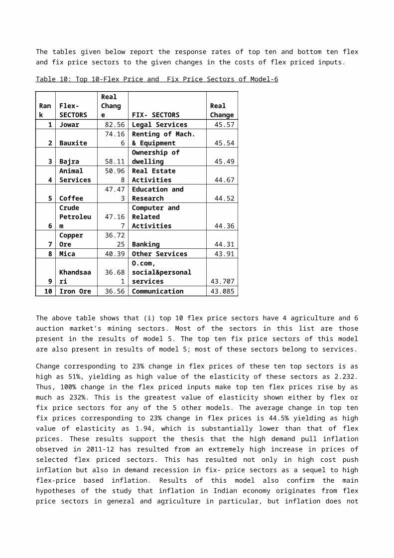
23. IMPACT OF CHANGE IN FLEX PRICES ON FIX PRICE SYSTEM: FLEX AND FIX PRICE MODEL 4 AND 6Results of descriptive statistics and ANOVA are reported in the tahle given below.

Table: 18: DESCRIPTIVE STATISTICS OF IMPACT OF CHANGES IN FLEX PRICE ON FIX PRICES (MODEL 4&6)

5%   10%   15%   23%  

            (Observed)  

Mean 4.535 Mean 9.053 Mean 13.55 Mean 20.08

Standard Error 0.039 Standard Error 0.079 Standard Error 0.12 Standard Error 0.24

Median 4.608 Median 9.188 Median 13.75 Median 20.44

Mode #N/A Mode #N/A Mode #N/A Mode #N/A

Standard Deviation 0.366 Standard Deviation 0.743 Standard Deviation 1.15 Standard Deviation 2.27

Sample Variance 0.134 Sample Variance 0.551 Sample Variance 1.33 Sample Variance 5.14

Kurtosis 3.457 Kurtosis 3.707 Kurtosis 3.47 Kurtosis 6.30

Skewness -1.487 Skewness -1.529 Skewness -1.49 Skewness -1.83

Range 2.056 Range 4.206 Range 6.47 Range 14.18

Minimum 2.935 Minimum 5.776 Minimum 8.53 Minimum 8.76

Maximum 4.991 Maximum 9.981 Maximum 15.00 Maximum 22.94

Sum 403.641 Sum 805.685 Sum 1206.25 Sum 1787.54

Count 89 Count 89 Count 89 Count 89

As the calculated value of t of differences of mean and median are consistently less than 1.96 the differences are not significant. Therefore the distribution of impact of flex on fix prices at varying rates is more or less symmetrically distributed. The value of CV also declines from lower to higher rates of change in flex prices. Thus, this pattern conforms to the pattern of distribution of impact of flex on flex prices as well as the distribution pattern of results of model 3 and 5.

Table 19: TWO FACTORS ANNOVA: EFFECT OF FLEX PRICES ON FIX PRICE SYSTEM (MODEL 4&6)

ANOVA

Source of Variation SS Df MS F P-value F crit

Rows 419.07 88.00 4.76 5.96 0.00 1.32

Columns 11751.09 3.00 3917.03 4904.98 0.00 2.64

Error 210.83 264.00 0.80      

Total 12380.99 355.00        

Results of two factors ANOVA confirm that the changes in flex prices decisively affect the changes in flex prices; though magnitudes of changes differ between the rates and sectors significantly. These results are also in conformity with earlier results of previous model.

24. COMPARATIVE ANALYSIS OF RESPONSIVENESS OF FLEX AND FIX PRICES TO CHANGES IN FLEX PRICES (ALL FOUR MODELS)

The following three questions are answered in this section on the basis of empirical results derived from the application of all four models: (i) Are flex prices more responsive to change in flex prices or fix prices are more responsive to changes in flex prices (ii) Do different rates of change (s) in flex prices evoke significantly different rates of change in flex and fix price systems. In other words, do the elasticity of flex and fix prices with respect to changes in flex prices differ significantly between the rates? If the answer is affirmative then arc rather than point elasticity will serve the purpose better. The analysis focuses on both these aspects; (iii) last and more important question is which of the models furnishes better explanation of transformation of demand pull into cost push inflation. The model which emerges as the answer to the question will also be suitable for forecasting.

The answer to the first question is conclusively derived from a perusal of elasticity of flex prices with respect to their own change at different rates; set of elasticity at different rates of changes are compared with the corresponding elasticity of fix prices at the rates at which elasticity of flex prices are calculated. Column 1 of table 6.14 and 1.16 show that the elasticity both of flex and fix prices does not differ substantially between the rates; it implies that elasticity coefficients are quite stable. Therefore, average of elasticity at different points within an arc will almost equal the point elasticity both for flex and fix prices. The elasticity of fix prices at different rates are much lower than those of flex prices. These two inferences lead to the conclusion that increase in flex prices become self-feeding and there is a tendency of demand pull inflation to be transformed into cost push inflation in Indian economy. This is supported by elasticity coefficients in column 1 of these two tables. These results relate to Decomposed Model (Model 3).

Second columns of tables 6.14 and 6.16, pertaining to Integrated Model-4, shows that flex prices are more responsive than fix prices to changes in flex prices. This result in consonance with that of model 3. But elasticity coefficients of flex prices of Model 3 are a bit greater than the corresponding elasticity coefficients of flex prices of Model 4. Besides, the differences of elasticity coefficients of flex relative to fix prices are greater for Model 3 than 4.

Model 5 and 6 slightly differ from the models 3 and 4 because these models have been applied to the observed changes in flex prices in 2011-12. This is different from the application of other models to ad hoc changes of 5, 10 and 15% changes in flex prices, used in model 3 and 4. The columns 4 and 5 of the tables 6.14 and 6.16 highlight the following pattern of change in flex and fix prices: (i) Average of elasticity of all flex prices is far greater than the average of elasticity of all fix prices. Besides, the magnitude of difference of elasticity between flex and fix prices of Models 5 and 6 are much greater than the differences of Model 3 and 4. Besides, the elasticity coefficient of flex prices of model 5 is greater than that of model 6. However the elasticity coefficient of fix prices of Model 6 is a little bit greater than that of Model 5.

Elasticity coefficient of Models 5 and 6 are greater than corresponding elasticity coefficient of flex prices of Model 3 and 4. These results provide empirical evidence to support Marshal (1891/1962) that elasticity coefficients tend to be greater at higher than lower prices. Models 5 and 6 have been estimated at observed prices of 41 commodities, average of which is 23%. This is obviously much greater than 5, 10 and 15 % rates of changes considered in Models 3 and 4.

Table 20: Elasticity Coefficients of Flex Prices

  Model 3 (D) Model 4(F-F) Model 5 (D) Model 6 (F-F)

5% 1.30 1.097  NA  NA

10% 1.31 1.099  NA  NA

15% 1.32 1.101  NA  NA

23% (Observed)  NA  NA 1.353 1.126

Table 21 Elasticity’s of Fix Prices

  Model 3 (D) Model 4(F-F) Model 5 (D) Model 6 (F-F)

5% 0.8503 0.907    

10% 0.847 0.905    

15% 0.843 0.903    

23% (Observed)     0.796 0.873

Identification of Greatest and Least Sensitive Flex Price Sectors Common in all four Models

The effect of 5, 10 and 15% rates of change in flex prices on flex price system of all four models are shown in Table 6.17. The sectors shown in red colorare found most sensitive; the sectors in green color are least affected by the given rates of increase in flex prices. The most highly sensitive sectors to changes in flex prices in all 4 models are Paddy, Jowar, Bajra, Pulses, Animal Services, Other Live Stock Products, Bauxite , Sugar, Khandsari , Hydrogenated Oil and Edible oils. Of these 11 sectors, 4 are agriculture, 2 are animal husbandry sectors, while 1 sector is based on mining operations and 4 are agro-based industries. All these sectors approximate the theoretical thrust of the thesis. These sectors also furnish empirical evidence to the hypothesis that inflation in India originates from agriculture in general and food grains in particular. Paddy is the most commonly food item used in India and this is commonly present in the budget of all households. Besides, a very high proportion of demand for paddy originates from milling for processing. It is rice which is consumed not Paddy as such. So, even the slightest fall in output of Paddy results in high inflation. Jowar and Bajra are coarse grains, whose prices are directly affected by the change in prices of wheat and paddy because allocation of land for cultivation depends on relative rather than absolute prices (For detail see. Prakash, Buragohain and Sharma, 1992). Pulses, Hydrogenated oils and edible oils

and other animal products all constitute a part of protective foods. With the growth of income in general increase in the size of middle income group and reduction in the incidence of poverty in particular. The demand for these goods has been expanding exponentially a head of supply partly because of stagnating yield rates due to want of upgradation of Green Revolution Technology. Bauxite is also a part of flex price system and some of the mining products like Iron ore, Bauxite, Mica and Rare Earths. These constituents export items and face competition in export markets. Bauxite is an item which may not be subject to such competition in export markets besides demand for industrial use has also been increasing more rapidly than output.

The least sensitive flex price sectors to the designated rates of changes are the following flex price sectors: Sugarcane, Cotton, Tobacco, Coal Lignite, Natural Gas, Iron Ore, Manganese Ore, Mica and Other Non-Metallic Mineral in all four models. Three of these sectors are related to agriculture; all these three crops are commercial crops. Tobacco and tobacco products have been under stringent control. For example smoking in public places has been prohibited. Consequently, demand for tobacco and tobacco product has been declining globally and heavy taxation has resulted in high prices of these goods already. So, state of demand in the market make producers reluctant to raise prices easily. Cotton constituent an essential intermediate input of textile industry which, has been moving away from production of pure cotton textiles to mixed stuff. This is an international scenario both cotton and cotton textiles are also a part of exports which are subject to international influences. Sugarcane is an essential input of sugar industry which has been a child of protection for a pretty long time since its birth in early 1930’s. For nearly two decades, sugar industry has been subject to dual pricing policy. Besides, there is a sugar syndicate in India which always waits for an opportunity to get speculative gains. But, 2008 has been a year of Global economic slowdown. Besides, sugar is also been exported periodically. So, the sugar prices are subject to three fold forces (i) Domestic state of supply and demand (ii) Policy Interventions and (iii) International movements in Sugar prices. Rests are the mining sectors, which do not require agro materials as inputs. So, their prices are less sensitive to changes in agricultural based flex prices. Whatever changes have occurred in the prices of these sectors are accounted partly by wage and interest rates hikes and general inflationary expectations.

FINDINGS AND CONCLUSIONS

The following are the important findings and inferences drawn from the results:

(i) The loss of information involved in decomposition of an integrated input output model leads to the loss of certain degree of generality of the results;

(ii) Different ways of combining decomposed components make the results of one model differ from those s of other decomposed models;

(iii) The results of analysis have provided an extensive and conclusive empirical evidence to support the thesis that inflation in Indian economy begins from flex price sectors in general but from such agriculture sectors as cereals, pulses, fruits, vegetables, milk and milk products etc. Inflation percolates to other segments of agriculture such as commercial crops from above sectors;

(iv) Prevailing conventional concept of inflation needs radical change to encompass structural inflation. Conventionally, demand pull inflation represents that state of the economy in which too much money chases too few goods. In this case, no particular set of goods is specified to be chased by too much money. Structural approach to inflation requires this. Inflation in India occurs whenever crop failure occurs which results in the shrinking of real output and decrease in monetary and real farm incomes.

(v) Buyers have to spend more money to buy food grains and other essential agricultural goods like vegetables, pulses and fruits, milk and milk product etc. which also reduces monetary income available for spending on non-agricultural goods. It causes demand recession in fix-price sectors. This also explains the existence of recession in fix-price sectors, especially manufacturing even when the economy is in the grip of inflation;

(vi) This genre of demand pull inflation makes agro-raw materials and other inputs of production costlier than before. This makes the cost of production rise evading to cost push inflation.

(vii) Wages and interest rates also rise in the inflationary spiral which further accentuates the cost push inflation. These results of this paper lend credible evidence to substantiate this hypothesis. Therefore, it may be concluded that demand pull inflation is finally transformed into cost push inflation.

Notes

1. RBI has announced reduction in interest rate only recently in the first half of April, 2016. High interest rate policy has been followed till then to control inflation.

2. Flex and fix prices were initially identified in two exploratory exercises. First exercise showed 27 sectors as flex price sectors. These sectors were identified on a priori reasoning which conforms to flex-fix price theories (For details, see, Sudhi Sharma and Prakash, Shri, 2014). 14 more markets were identified as flex-price markets on the basis of observed prices being greater than the cost-based prices by more than 20%.

References

1. Books

Brittan, Arthur (1996) Social Structure and Structuralism, In Kooper, Adam and Kooper (Editors) The Social Science Encyclopedia Routledge

Brooks, Chris (2008) Introductory Econometrics for Finance, Cambridge University Press.

Campbell, J, MacKinlay (2007) The Econometrics of Financial Markets, New Age International Publications

Dumont, I. (1970/1966) Homo Hoierarchicus, London. {Cited from P.E. de Jessim de Jung}.

Frisch, Ragnar (1991) A Course in Econometrics, Harvard University Press, Cambridge.

Goldberger, A.S.(1969) Impact Multipliers of Regression, London

Gujarati, Damodar N. and Gunasekar, Sangeetha (2007) Basic Econometrics, Tata-McGraw Hill, Mumbai.

Harvey, A. C. (1980) On Comparing Regression Models in Levels and First Differences, International and Economic Review, 21, pp. 707-720

Harvey, A. C. (1981) Time Series Models, Phillips Allan and Humanities Press

Harvey, A.C. (1989) Forecasting, Structural Time Series Models and the Kalman Filter, Cambridge University Press.

Hicks, J.R. (1962) Theory of Wages, Basil Blackwell, London

Hicks, J.R. (1965) An Essay on Crisis in Keynesian Economics, Basil Blackwell, London.

Hicks, J.R.(1965) Capital and Growth, Oxford, London

Hrishman, A.O. (1958) Strategy of Economic Development, Yale University Press, New Haven, Connecticut, U.S.A.

Intriligator, M.D. (1985) Models and Methods of Econometrics, London

Jung, P.E. de Jessim de (1996) ‘structuralism’. Published in Kooper, Adam and Kooper, Jessica (Editors) The Social Science Encylopedia, Routledge, pp. 852-54

Kmenta, Jan (1986) Elements of Econometrics, Macmillan, New York.

Kuznets, Simon (1966) Modern Economic Growth- Rate, Structure and Speed, Yale University Press, New Haven, Connecticut, U.S.A.

Lewis, A (1962) Theory of Economic Growth, Allen Unwin, Landon

Mathur, P. N. (1986) Schism in Indian Polity and Gandhi, NEHU Publications, Shillong.

Mathur, P.N. (1992) Why Developing Countries Fail to Develop? Mc Millan, Landon

Popper, Karl (1968) The Logic of Scientific Discovery, third edition, Routledge, London

Wallice, K. E. (1972) Introduction to Econometrics, London.

Harvey, A. C. (1980) On Comparing Regression Models in Levels and First Differences, International and Economic Review, 21, pp. 707-720

Harvey, A. C. (1981) Time Series Models, Phillips Allan and Humanities Press

Harvey, A.C. (1989) Forecasting, Structural Time Series Models and the Kalman Filter, Cambridge University Press.

Hicks, J.R. (1962) Theory of Wages, Basil Blackwell, London

Hicks, J.R. (1965) An Essay on Crisis in Keynesian Economics, Basil Blackwell, London.

Hicks, J.R.(1965) Capital and Growth, Oxford, London

Hrishman, A.O. (1958) Strategy of Economic Development, Yale University Press, New Haven, Connecticut, U.S.A.

2. Ph.D.Theses:

Anita (1982) Behavior of Fix Prices in Indian Economy, M.Phil Thesis, Punjabi University, Patiala.

Bhatt Joshi, Niharika (2015) Organization Structure and Productivity of SMEs-A Study of Light Electrical Goods Industries of India, Ph.D. Thesis, BIMTECH/MLSU. Udaipur

Buragohain, Taru Jyoti (1994) Marketed Surplus, Output and Prices of Food Grains in Indian Economy, Ph. D. Thesis, Economic Department, NEHU , Shillong

Choudhary, Sumitra (1994) Price and Output Movements of Engineering and Chemical Goods Industries in Indian Economy, Ph.D. Thesis, Economics Department, NEHU, Shillong.

Goel, Veena (1983) Marketed Surplus, Intermediate Traders Stocks and their influence on Prices: A Study of Mandies of Patiala” M.Phil Thesis, Punjabi University Patiala.

Goel, Veena (1986) Price and Output Movements of Agro- Based Industries, Ph.D. Thesis, Economics Department, NEHU, Shillong.

Buragoahin, Taru Jyoti (1995) Marketed Surplus and Agricultural Prices in Indain Economy, Ph.D. Thesis, Economics Department, NEHU, Shillong.

Rani, Sushma (1983) Marketed Surplus and Consumption of Food Grains: A Comparative Study of Farm Households of Haryana and Punjab, M.Phil Thesis, Punjabi University Patiala

Sen Gupta, Keya (1993) Price and Output Determination of Agro-Linked Industries in Indian Economy, Ph.D. Thesis, Economics Department, NEHU, Shillong.

Sharma, Ritu (2014) Analysis of Households’ Choice between Current and Future Consumption Expenditure: A Study of National Capital Region of Delhi, Ph.D. Thesis, Mysore University, Center of Research BIMTECH, Greater Noida.

Sharma, Shalini, (2004) Empirical Analysis of Determination of Agriculture Prices in Indian Economy, Ph.D. Thesis, Aligarh Muslim University.

Tripathi, Indu Bala (1982) Marketed Surplus, Consumption of Self Produced Food Grains and Prices, M.Phil Thesis, Punjabi University Patiala.

3. Research Papers:

Abramowitz, N (1956) Resources and Output Trends in the United States since 1870’s, American Economic Review, Papers and Proceedings, Vol. 46, pp. 5-23.

Agarwal, P and Kumarasamy, D (2012) Food Prices Inflation in India: Causes and Cures, IEG, Working paper no. 318

Anita (1984) Cost-Price Adjustment in Indian Manufactures- A Study of Wage-Cost of Interrelations of Agro- Based Industries of India, NEHU Journal of Social Sciences, Vol.2, Issue-2

Anita (1984), Behavior of Fix Prices in Indian Economy, NEHU Journal of Social Sciences, Vol.II.

Ball, Chari and Mishra (2015), Understanding Inflation in India, India Policy Forum, NCAER, New Delhi

Bhanumurthy, N.R., Das, Surajit and Bose, Sukanya (2005), Oil Price Shock and Its Impact on India, Sanei: Working Paper Series no.12 – 05.

Bhattacharya, Rao and Gupta, A. (2014) Understanding Food Inflation in India, ADB South Asia, Working Paper series.

Bhowmik and Debesh (2013) An Econometric Model of Inflation in India, International Journal of Scientific and Research Publications, Vol.5, Issue.2

Cristardoro, R and Veronese, G (2011) Monetary Policy in India: Is Something Amiss? Indian Growth and Development Review, Vol.4, No.2, pp.166-192

Dua, P. Raje and Sahoo (2008) Forecasting Interest Rate in India, The Journal of Applied and Economic Research, MARGIN

Goel, Veena (1986) Determination of Agricultural Price in Mandies of Patial District, VARTA, Vol.7, Issue-1

Jha, Shikha and Mundle, Sudipto (1987) Inflationary Implications of Mobilisation Resources through Administered Price Increases, Chapter in New Series in Policy Studies, NIPFP, New Delhi.

Kaur and Savneet (2013) Inflation- Impact on Indian Economy and Agriculture, International Journal of Scientific and Engineering Research, Vol.4, Issue.7

Mathur, P. N. and Prakash, Shri (1986) Inventory Behavior of Indian Agriculture and its Impact on General Price Level in Indian Economy, Journal of Engineering and Economics, Elsevier. Republished in Chikan, Attila (Editor) Economics and Management of Inventory, Part II, Hungarian Academy of Science and Elsevier.

Mathur, P.N. (1962) An Efficient Path for the Technological Transformation of an Economy. In Barna, Tibor (Editor), Structural Interdependence and Economic Development, Mc Million London.

Mathur, P.N. (1975), Tracing the Economic Impact through the Commodity Quantity Structure- New Approach to Empirical Analysis of Inflation, Un-utilised Capacity etc. by combining Flex and Fix Price Analysis, 5th National Confernce, IIORA, Ahemdabad.

Mathur, P.N. and Ezekeil (1961) Marketable Surplus of Food and Price Fluctuations in a Developing Economy, Kyklos, Vol.16, Pg. 396-408

Mathur, P.N. and Prakash, S. (1980) Invetory Behaviour of Indian Agriculture and its Effects on General Price Level. In Chikan, A. (Editor) Economic and Management of Inventories, Part A, Elseviere and Hungarian Academy of Science, Budapest.

Mishra, Mahima and Walvekar. Shubhangi, (2014) “India’s Monetary Policy and Rising Food Inflation”, Working Paper, National Institute of Public Finance and Policy, New Delhi.

Mohanty, Upendra Nath (2001) Impact of Margins on Cost and Price of Jute Textiles Industry of India, Business Perspectives, Vol. III.

Morishima, M. (1952) On the laws of change of price system in an economy which contains complementary commodities, Osaka Economic Papers.

Paramanik and Kamaiah (2014) A Structural Vector Auto regression Model for Monetary Policy Analysis in India, The Journal of Applied and Economic Research, MARGIN, pp.401-429

Parvathamma, G.I. (2014) A Review on Inflation in India- Causes, its impacts, Trends and Measures to Control, Indian Journal of Applied Research, Vol.4, Issue.9

Prahash, Shri and Goel, Veena (1987) Price and Output Movement of Agro- Based Industries in Indian Economy, Published in Mahajan, V.S. (Editior) Studies In Industrial Economy of Indian, Vol.2, Deep and Deep Publications

Prakash, S , Buragohain, T. J. and Sharma, A (1992) Determination of Allocation of Area for Cultivation Under Different Crops and Related Price Diffrentials, Journal of Development Alternatives, Zurich

Prakash, S and Arora Bhatia, Chitra (2013) Determination of Opening Prices of Equities of the Day, Journal of Applied Finance and Banking, Vol.3, Issue.4, pp.199-228, U.K.

Prakash, S and Goel, Veena (1987) Marketed Surplus, Traders’ Stocks and Prices of Food Grains: A Study of Wheat in Patiala Mandies. In Chikan, A. (Editor), Recent Advances in Inventory Research, Elseviere

Prakash, S and Tripathi, Indu Bala (1977) Marketed Surplus and Consumption of Food Grains- A Study of Farm Household’s Behaviour in Punjab, In. Singh, Tarlok (Editor), Research on Poverty in India, Concept.

Prakash, S. and Goel, Veena (1985) Price and Output Movements of Agriculture in Indian Economy. In Mahajan, V. S. (Editor) Studies in Indian Agriculture, Deep & Deep, New Delhi.

Prakash, S. and Goel, Veena (1985) Price and Output Movements of Agro- Based Industries in Indian Economy. In Mahajan, V.S.(Editor) Studies in Industrial Economy of India, Deep and deep, New Delhi.

Prakash, Shri (1981) Cost- based Prices in Indian Economy, Malayan Economic Review, Vol.26, No. 1, Published as Leading Paper

Prakash, Shri (1986) Food Security, Public Stocks and Production of Food Grains in India: In Mahajan, V.S. (Editor) Studies in Indian Agriculture and Rural Development, Deep & Deep, New Delhi

Prakash, Shri (1986,1991), Generalized Dynamic Linkage Pattern as a base of Convergence of Unbalanced to Balance Growth Theory: Some Methodological and Theoretical Issues with Application to Indian Economy, International Journal of Development Planning Literature, Vol. 6, Nos 3-4, July-Oct. Also Presented at International Conference on Input Output Techniques, Sapporo (Japan) 1986

Prakash, Shri (2013) Revisiting Flex-Fix Dichotomy of Price Behavior, Persistent High Inflation and Sluggish Economic Growth in Globalized Indian Economy, VARTA, October, No.2, Vol.XXXIV. Based on Kautilaya Award Address to the UPUEA’s Conference

Prakash, Shri and Goel, Veena (1988) Marketed surplus, Farm Prices and Stocking behavior of food grain traders in Mandies of Patiala District. Published in Chikan, Attila (Editor) “Recent Advances in Economics and Management of Inventories”, Hungarian Academy of Sciences, Budaopest

Prakash, Shri and Rajan, P. (1977) Prices and Output of Agriculture and Growth of Indian Economy, The Indian Journal of Economics, October.

Prakash, Shri and Sharma, Ritu (2015) Multiplier Effect of Consumption on Growth of Income and Investment: Analysis of Sequential Rounds in Input Output Framework, The Indian Journal of Economics, Vol.XCV, No. 378, Part III

Prakash,S and Balakrishnan, B (2006) Development and Growth- Convergence of Macro Towards Micro Theory: A Managerial Approach to Conceptualisation, Business Perspectives, Vol. 8, Pg. 39-57

Rao,N., Reddy,P., Basha, et.al (2013) A Study of Inflation in India, International Journal of Social Sciences, Vo. 2

Sabade, Shubhada (2013) Is Money Supply the Cause of Inflation in India? An Alternative Postulate to Understand Inflation, Procedia Social and Behavioural Sciences, Elsevier, pp.379-382

Sharma, Samit (2001) Imaoct of Margins on Cost and Prices of Manufacturing Industries of India, Business Perpectives, Vol.3, No.2, July December

Sharma, Samit and Mohanty, N.K. (2009) Trade, Transport and Tax Margins in Jute and Mesta Textile Industries of India, Business Perspectives. Vol. VIII, No.1.

Sharma, Sudhi, Prakash, Shri and Negi, Gautam (2015), Agriculture, Non Agriculture and General Inflation in Indian Economy from 1867 to 2013. Presented at the 18th National Conference of IORA on Input Output and Related techniques, BIMTECH, Greater Noida.

Singh, Karan (2012) An Assessment of Inflation Modeling in India, Indian Council for Research on International Economic Research, Working paper 259

Singh, Pratima (2011) Inflation in India: An Empirical Analysis, ISAS Working paper, National University of Singapore.

Venkatramaiha, P.V. (1967) Margins in Indian Industries. Published in Mathur, P.N. and Bharadwaj, R. (Editors) Economic Analysis in Input Output Framework, Volume I, Input Output Research Association, GIPE, Pune.

Appendix- Tables 1

Steps involved in the application of the decomposed models

1. First of all the prices of all four segments are calculated without introducing any change in the prices of 2007-08 in which the transaction and other tables are given. These prices constitute the base for comparison with prices derived from the application of alternative models developed in the paper.

2. The first experiment is conducted with 5% constant increase in the prices of all 27 flex price sectors. The application comprises following steps. 2.1 Values of flex price inputs supplied to all sectors of the economy in segment 1 and segment 2 are

increased by 5%.2.2 Corresponding changes are made in output vector of 27 flex price sectors. 2.3 A new coefficient matrix has been calculated of 130* 130 matrix2.4 Now, (I-A)-1 is derived from these new coefficient matrix.2.5 Value added vector of four segments is determined separately on the principle of proportionality. The

ratio of sum total of inputs coefficient of first and third segments is used to split value added of flex price sector into two parts corresponding to first and third segments. The value added vector of fix price sector is also split analogously in to two parts corresponding to second and fourth part.

2.6 Inverse matrix is also decomposed into four parts corresponding to four segments that are Inverses of first and four segments is 27* 27 and 103*103 square matrix respectively. These are used for pre multiplication by corresponding value added vectors.

2.7 However, inverses of second and third segments are non square matrix. So, to make them confirm for multiplication to the corresponding value added vectors. A null sub matrix is used to augment these inverses to make them of requisite order.

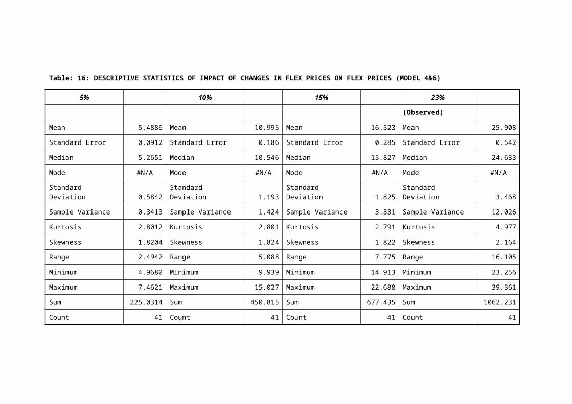
2.8 The components of value added vectors have already been augmented as mentioned in the assumptions.

2.9 The prices have been derived as usual procedure, pre multiplication of inverse by value added vector.2.10 The same steps have been replicated in the application of other decomposed models