X-ray,UV andopticalanalysisofsupergiants: Ori - arXiv¬rst estimates for M were derived assuming...
33
arXiv:1511.09365v2 [astro-ph.SR] 1 Dec 2015 MNRAS 000, 1–29 (2015) Preprint 2 December 2015 Compiled using MNRAS L A T E X style file v3.0 X-ray, UV and optical analysis of supergiants: ǫ Ori Raul E. Puebla, 1⋆ D. John Hillier, 1 Janos Zsarg´ o, 2 David H. Cohen 3 and Maurice A. Leutenegger 4,5 †‡§ ¶ 1 Department of Physics and Astronomy & Pittsburgh Particle Physics, Astrophysics, and Cosmology Center (PITT PACC), University of Pittsburgh, 3941 O’Hara Street, Pittsburgh, PA 15260, USA. 2 Escuela Superior de F´ ısica y Matem´ atica. Instituo Polit´ ecnico Nacional. Av. Instituto Polit´ ecnico Nacional, Edificio 9, C.P. 07738, M´ exico, DF. M´ exico. 3 Department of Physics and Astronomy. Swarthmore College, 500 College Ave. Swarthmore, PA 19081, USA. 4 CRESST/University of Maryland, Baltimore County, 1000 Hilltop Circle, Baltimore, MD 21250, USA. 5 NASA/Goddard Space Flight Center, 8800 Greenbelt Road, Greenbelt, MD 20771, USA. ABSTRACT We present a multi-wavelength (X-ray to optical) analysis, based on non-local thermodynamic equilibrium photospheric+wind models, of the B0 Ia-supergiant: ǫ Ori. The aim is to test the consistency of physical parameters, such as the mass-loss rate and CNO abundances, derived from different spectral bands. The derived mass-loss rate is ˙ M/ √ f ∞ ∼1.6×10 −6 M ⊙ yr −1 where f ∞ is the volume filling factor. However, the S iv λλ1062,1073 profiles are too strong in the models; to fit the observed profiles it is necessary to use f ∞ <0.01. This value is a factor of 5 to 10 lower than inferred from other diagnostics, and implies ˙ M 1×10 −7 M ⊙ yr −1 . The discrepancy could be related to porosity-vorosity effects or a problem with the ionization of sulfur in the wind. To fit the UV profiles of N v and O vi it was necessary to include emission from an interclump medium with a density contrast (ρ cl /ρ ICM ) of ∼100. X-ray emission in H-He like and Fe L lines was modeled using four plasma components located within the wind. We derive plasma temperatures from 1 ×10 6 to 7 ×10 6 K, with lower temperatures starting in the outer regions (R 0 ∼3-6 R ∗ ), and a hot component starting closer to the star (R 0 2.9 R ∗ ). From X-ray line profiles we infer ˙ M < 4.9×10 −7 M ⊙ yr −1 . The X-ray spectrum (0.1 kev) yields an X-ray luminosity L X ∼ 2.0 × 10 −7 L bol , consistent with the superion line profiles. X-ray abundances are in agreement with those derived from the UV and optical analysis: ǫ Ori is slightly enhanced in nitrogen and depleted in carbon and oxygen, evidence for CNO processed material. Key words: stars: supergiants, massive, mass-loss, abundances – techniques: spec- troscopic, X-rays, ultraviolet, optical – X-rays: stars – stars: individual: ǫ Ori. ⋆ E-mail: [email protected] † Based on observations obtained with XMM-Newton, an ESA science mission with instruments and contributions directly funded by ESA Member States and NASA. ‡ The scientific results reported in this article are based on data obtained from the Chandra Data Archive. § Some of the data presented in this paper were obtained from the Mikulski Archive for Space Telescopes (MAST). STScI is oper- ated by the Association of Universities for Research in Astronomy, Inc., under NASA contract NAS5-26555. Support for MAST for non-HST data is provided by the NASA Office of Space Science via grant NNX09AF08G and by other grants and contracts ¶ Optical data for this work were obtained from POLARBASE (Petit et al. 2014) 1 INTRODUCTION Massive stars play a fundamental role in the Universe. Con- sidered the progenitors of core collapse supernovae, they are also responsible for galactic H ii regions, the transfer of mass, momentum and energy to the interstellar medium (ISM), and for metal enrichment in their host galaxy. Among the stellar wind properties, the mass-loss rate ( ˙ M) is crucial for understanding the evolution of massive stars. ˙ M affects the star’s lifetime on the main sequence, the rotation rate of the star, and the star’s subsequent evolution (e.g. Chiosi & Maeder 1986; Maeder & Meynet 2000). The first estimates for ˙ M were derived assuming spherical smooth winds. However, subsequent observations reveal inconsisten- cies. For instance, the far UV resonance line profiles (e.g. c 2015 The Authors
Transcript of X-ray,UV andopticalanalysisofsupergiants: Ori - arXiv¬rst estimates for M were derived assuming...

arX
iv:1
511.
0936
5v2
[as
tro-
ph.S
R]
1 D
ec 2
015
MNRAS 000, 1–29 (2015) Preprint 2 December 2015 Compiled using MNRAS LATEX style file v3.0
X-ray, UV and optical analysis of supergiants: ǫ Ori
Raul E. Puebla,1⋆ D. John Hillier,1 Janos Zsargo,2 David H. Cohen3
and Maurice A. Leutenegger4,5†‡§ ¶1Department of Physics and Astronomy & Pittsburgh Particle Physics, Astrophysics, and Cosmology Center (PITT PACC),University of Pittsburgh, 3941 O’Hara Street, Pittsburgh, PA 15260, USA.2Escuela Superior de Fısica y Matematica. Instituo Politecnico Nacional. Av. Instituto Politecnico Nacional, Edificio 9,C.P. 07738, Mexico, DF. Mexico.3Department of Physics and Astronomy. Swarthmore College, 500 College Ave. Swarthmore, PA 19081, USA.4CRESST/University of Maryland, Baltimore County, 1000 Hilltop Circle, Baltimore, MD 21250, USA.5NASA/Goddard Space Flight Center, 8800 Greenbelt Road, Greenbelt, MD 20771, USA.
ABSTRACT
We present a multi-wavelength (X-ray to optical) analysis, based on non-localthermodynamic equilibrium photospheric+wind models, of the B0 Ia-supergiant: ǫ Ori.The aim is to test the consistency of physical parameters, such as the mass-loss rateand CNO abundances, derived from different spectral bands. The derived mass-lossrate is M/
√f∞ ∼1.6×10⁻⁶ M⊙ yr−1 where f∞ is the volume filling factor. However,
the S iv λλ1062,1073 profiles are too strong in the models; to fit the observed profiles itis necessary to use f∞ <0.01. This value is a factor of 5 to 10 lower than inferred fromother diagnostics, and implies M . 1×10⁻⁷ M⊙ yr−1. The discrepancy could be relatedto porosity-vorosity effects or a problem with the ionization of sulfur in the wind. To fitthe UV profiles of Nv and Ovi it was necessary to include emission from an interclumpmedium with a density contrast (ρcl/ρICM ) of ∼100. X-ray emission in H-He like andFe L lines was modeled using four plasma components located within the wind. Wederive plasma temperatures from 1×10⁶ to 7×10⁶ K, with lower temperatures startingin the outer regions (R0 ∼3-6 R∗), and a hot component starting closer to the star
(R0 .2.9 R∗). From X-ray line profiles we infer M < 4.9×10⁻⁷ M⊙ yr−1. The X-rayspectrum (>0.1 kev) yields an X-ray luminosity LX ∼ 2.0× 10⁻⁷Lbol, consistent withthe superion line profiles. X-ray abundances are in agreement with those derived fromthe UV and optical analysis: ǫ Ori is slightly enhanced in nitrogen and depleted incarbon and oxygen, evidence for CNO processed material.
Key words: stars: supergiants, massive, mass-loss, abundances – techniques: spec-troscopic, X-rays, ultraviolet, optical – X-rays: stars – stars: individual: ǫ Ori.
⋆ E-mail: [email protected]† Based on observations obtained with XMM-Newton, an ESAscience mission with instruments and contributions directlyfunded by ESA Member States and NASA.‡ The scientific results reported in this article are based on dataobtained from the Chandra Data Archive.§ Some of the data presented in this paper were obtained from theMikulski Archive for Space Telescopes (MAST). STScI is oper-ated by the Association of Universities for Research in Astronomy,Inc., under NASA contract NAS5-26555. Support for MAST fornon-HST data is provided by the NASA Office of Space Sciencevia grant NNX09AF08G and by other grants and contracts¶ Optical data for this work were obtained from POLARBASE(Petit et al. 2014)
1 INTRODUCTION
Massive stars play a fundamental role in the Universe. Con-sidered the progenitors of core collapse supernovae, they arealso responsible for galactic H ii regions, the transfer of mass,momentum and energy to the interstellar medium (ISM),and for metal enrichment in their host galaxy.
Among the stellar wind properties, the mass-loss rate(M) is crucial for understanding the evolution of massivestars. M affects the star’s lifetime on the main sequence, therotation rate of the star, and the star’s subsequent evolution(e.g. Chiosi & Maeder 1986; Maeder & Meynet 2000). Thefirst estimates for M were derived assuming spherical smoothwinds. However, subsequent observations reveal inconsisten-cies. For instance, the far UV resonance line profiles (e.g.
c© 2015 The Authors

2 Raul E. Puebla et al.
Pv and S iv) observed by COPERNICUS and FUSE can-not be simultaneously fit with Hα (e.g. Crowther et al. 2002;Hillier 2003). Futhermore, P Cygni profiles from highly ion-ized species, such as Nv and Ovi, were detected in the UVspectrum (Snow & Morton 1976), but such ionization statesare incompatible with radiative equilibrium in a smoothwind. Cassinelli & Olson (1979) suggested that these ionscould be produced by Auger ionization by X-rays (doubleionization due to ejection of an inner shell electron by aX-Ray photon.), a suggestion confirmed by Einstein X-rayObservatory which found that massive stars are strong X-ray sources (Harnden et al. 1979; Seward et al. 1979). Twoscenarios were proposed to explain the observed X-ray emis-sion: emission from a corona just above the photosphere(Hearn 1975; Cassinelli & Olson 1979) and X-ray emissionfrom shock-heated plasma distributed throughout the wind(Lucy & White 1980; Lucy 1982; Owocki et al. 1988). Thelatter is now generally accepted as the dominant X-ray emis-sion mechanism in single stars.
Because of the deficiencies discussed above, the “stan-dard” smooth wind model needed to be revised. Atpresent, it is widely accepted that the winds of mas-sive stars are strongly structured (clumped). The exis-tence of such winds is supported by hydrodynamical time-dependent simulations that predict that radiation-drivenwinds are unstable (Owocki et al. 1988; Feldmeier et al.1997; Runacres & Owocki 2002). Evidence for these inho-mogeneities has been found, for instance, by observations ofvariable discrete absorption components (DAC) in UV andoptical lines (e.g. Fullerton et al. 1996; Kaper et al. 1996;Morel et al. 2004; Prinja et al. 2006), and from observationsof stochastic variability (e.g., Eversberg et al. 1998). Hillier(1991) showed that the electron scattering wings of recom-bination lines of Wolf-Rayet (W-R) stars cannot be repro-duced by smooth winds, necessitating clumped models andlower mass-loss rates to fit them.
Clumping can be treated using two approximations.The simplest approach considers optically thin clumps atall wavelengths (“microclumping”). The second approach al-lows for the optical thickness of clumps, especially for lines(“macroclumping”). Commonly it is assumed that the inter-clump medium is void. However, recently it has been shownthat its influence is not negligible (e.g. Zsargo et al. 2008).
Microclumping has been used to lower the discrepancybetween Pv UV resonance lines and Hα. Typical filling fac-tors in O stars are 0.01 to 0.1, although, in some cases, it stillmay be necessary to reduce the P abundance by a factor of2 from the expected value (e.g. Crowther et al. 2002; Hillier2003; Bouret et al. 2005; Fullerton et al. 2006; Bouret et al.2012). The principal consequence of microclumping is a re-duction of mass-loss rates by factors from 3 to 10.
A 3D Monte-Carlo simulation performed bySurlan et al. (2013) showed that when macroclumpingis included the Hα and Pv lines discrepancy is fixedfor higher values of the volume filling factor, yieldinghigher mass-loss rates when compared with those basedon pure microclumping (see also Oskinova et al. 2007;Sundqvist et al. 2010; Surlan et al. 2012).
The problem with all these analyses is degeneracy –there are several parameters which can be varied but only afew lines that can be modeled, making it difficult to reachdefinitive conclusions (see details in Surlan et al. 2013).
As noted by several different authors (e.g. Cohen et al.2010), the fitting of X-ray lines provides an indepen-dent method to estimate the mass-loss rates of OBstars. Cohen et al. (2010) estimated the characteristic op-tical depth for X-rays (τ∗ = κM/4πR∗v∞), fitting sep-arately X-ray lines and then fitting the best opticaldepth wavelength distribution using the mass-loss rateas a free parameter. The main reported problem withX-ray line emission is that most of the observed pro-files are fairly symmetric. This contradicts models thatpredict lines skewed to the blue (Macfarlane et al. 1991;Owocki & Cohen 2001). Three explanations are currentlyproposed: resonance scattering, lower mass-loss rates andporosity (see Oskinova et al. (2011) for a summary ofX-ray emission properties of OB stars). However, reso-nance scattering cannot explain all observed line profiles(Ignace & Gayley 2002; Leutenegger et al. 2007), while theneeded reduction in the mass-loss rates inferred from Hαis large (factors of 2 to 10) (e.g. Cohen et al. 2014a). Ithas also been argued that the porosity lengths (a mea-sure of mean free path of photons between clumps) re-quired to get symmetric lines are unlikely to be as largeas needed (Owocki & Cohen 2006). Sundqvist et al. (2012)and Leutenegger et al. (2013) concluded that a porosity con-sistent with the observed X-ray line profiles cannot affectthe mass-loss rate determination significantly. Furthermore,Herve et al. (2013) showed that porosity is not important toexplain the X-ray spectrum of ζ Pup.
With the aim of providing more rigorous constraints,and reducing systematic errors, we present our work ona multi-wavelength analysis of the supergiant ǫ Ori. Theanalysis is based on X-ray data from Chandra and XMM-Newton, UV data from IUE, HST, and the COPERNICUSsatellite, and optical data taken from POLARBASE archive.The photospheric, wind and hot-plasma parameters are ob-tained from a modified version of cmfgen (Hillier & Miller1998), and the consistency of the derived parameters is ex-amined.
The paper is constructed as follows: In the next sec-tion, we present results from previous analyses of ǫ Ori andits main spectral features. Observational data are describedin Section 3 while the method and model assumptions arepresented in Section 4. The results of optical, UV and X-rayanalysis are given in Section 5. A discussion of the resultsand conclusions are provided in Sections 6 and 7.
2 ǫ Ori (HD 37128)
The B0 Ia supergiant star ǫ Ori (HD 37128) is the centralstar of the Orion Belt, and is also known as Alnilam (anArabic word that means “string of pearls” (Knobel 1909))and belongs to the Orion OB1(b1) association.
The first attempts to derive the physical parameters forǫOri using photospheric models in non-local thermodynamicequilibrium (NLTE) were made by Auer & Mihalas (1972)and Lamers (1974) who used optical line profiles, and foundan effective temperature around 29000 K and log g=3.0.McErlean et al. (1998) using an NLTE model found similarparameters, while Kudritzki et al. (1999), using the originalversion of the code fastwind (Santolaya-Rey et al. 1997;Puls et al. 2005) found Teff=28000 K and log g=3.0.
MNRAS 000, 1–29 (2015)

X-ray, UV and optical analysis of supergiants: ǫ Ori 3
Crowther et al. (2006) and Searle et al. (2008) used theNLTE transfer code cmfgen (Hillier & Miller 1998) to de-rive effective temperatures of 27000 K and 27500 K respec-tively. However, there exists a discrepancy between theirlog g values – Crowther et al. reported a value of 2.9 whileSearle et al. reported 3.1. Both works also analyzed theCNO abundances of ǫ Ori. In contrast to the nitrogen defi-ciency reported byWalborn (1976), Crowther et al. reporteda slight enrichment of nitrogen and depletion of carbon. Onthe other hand, Searle et al. found a nitrogen and carbondeficiency and a solar oxygen abundance.
Previous values for mass-loss rate from different di-agnostics encompass values from 1.5×10⁻⁶ to 4.3×10⁻⁶
M⊙ yr−1. Diagnostics include Hα strength (Kudritzki et al.1999; Crowther et al. 2006; Searle et al. 2008; Urbaneja2004), UV P Cyg profiles (Howarth & Lamers 1999), ther-mal radio fluxes (Blomme et al. 2002; Lamers & Leitherer1993) as well as H and He infrared lines in the H and Kbands (Repolust et al. 2005; they derived an upper limit ofM=5.25×10⁻⁶ M⊙ yr−1). These values where derived usingsmooth winds. In a subsequent analysis by Najarro et al.(2011), lines from the L band were used in conjunctionwith UV and optical data to obtain a mass-loss rate ofM/
√f∞=2.65×10⁻⁶ M⊙ yr−1 and a filling factor f∞=0.03.
Mass-loss rate determinations should all be scaled tothe same distance, since the mass-loss rate typically scalesas d1.5 for ρ2 dependent diagnostics (or d for ρ dependentdiagnostics such as X-ray profiles). Distance estimates forǫ Ori tend to cluster around 400 pc (Lesh 1968; Lamers 1974;Savage et al. 1977; Brown et al. 1994), and are broadly con-sistent with the initial HIPPARCOS determination of 412 pc(Perryman et al. 1997). However, with the latest calibrationthe new estimate is 606 pc (van Leeuwen 2007). This dis-tance is the highest ever estimated, and substantially in-creases the luminosity and mass-loss rate for ǫ Ori.
IUE and COPERNICUS spectra of ǫOri show line emis-sion from Nv and Ovi resonance transitions, which, giventhe effective temperature of ǫ Ori, provides evidence of X-rayemission in wind. Chandra and XMM spectra of HD 37128show strong emission lines from H/He-like atoms of C, N,O, Ne, Mg and Si as well as Fexvii lines.
Previous analyses of X-ray emission from ǫ Ori founda wide spatial distribution of the hot plasma in the wind.Cohen et al. (2014a) fitted Chandra lines and did notfind any correlation between the onset radius for emittingplasma and the emitting ion. This confirmed the results byLeutenegger et al. (2006) who found no evidence for differ-ent spatial distributions for different ions.
Recently, Cohen et al. (2014a) estimated the mass-lossrate for ǫ Ori by fitting X-ray line profiles. They reported twovalues of mass-loss rate: 2.1×10⁻⁷ M⊙ yr−1 and 6.5×10⁻⁷
M⊙ yr−1. The first value uses nine X-ray lines while thesecond value excludes three lines that might be influencedby resonance scattering.
ǫ Ori shows spectral variability in both the optical andUV. The main variability detected in the UV is associatedwith DACs, especially in the blue wing of the Si iv and Nv
doublets. Some other UV lines, including string photosphericlines, also show variability (Prinja et al. 2002). In the opti-cal Hα shows strong variability with changes in both shapeand strength occurring on a time scales of hours to tensof days (e.g. Ebbets 1982; Morel et al. 2004; Prinja et al.
2004; Thompson & Morrison 2013, and references therein).One possible cause of the variability is radial and non-radial oscillations that produce a mass-loss rate modulation(Thompson & Morrison 2013). Our calculations show thatvariations of ±30% in M about our derived value can explainthe observed variations of Hα.
We chose ǫ Ori as a standard early B supergiant dueto the availability of high resolution X-Ray, UV and opticaldata. In practice, spectral variability is common is B super-giants, and hence unavoidable. Its variability will introduceuncertainties in the derived wind parameters, but these un-certainties can be qualified, and will not affect our main aimof evaluating the consistency of the main physical parame-ters of ǫ Ori derived in this multi-wavelength analysis.
3 THE DATA
For this work we collected optical, UV and X-ray data fromdifferent archives as described below. The sources of the datais presented in Table 1.
3.1 Optical Data
The optical data were obtained from POLARBASE1, thestellar spectra archive for the NARVAL and ESPaDOnsechelle spectropolarimeters. The former is installed in theTelescope Bernard Lyot (TBL, Pic du Midi Observatory)and the latter at the Canada-French-Hawaii Telescope. Adetailed description of these instruments can be found inSilvester et al. (2012) and Petit et al. (2014). They are twinspectropolarimeters except for the aperture (2.8 arcsec forNARVAL and 1.6 arcsec for ESPaDOns). Both of them havea spectral resolution R=λ/∆λ ≃ 65000 and a spectral cover-age from 3690 to 10000 A. The wavelength calibration is per-formed using a Th-Ar spectra and it is refined using telluricbands as references for radial velocity. The instruments havetwo modes of operation: spectroscopic and polarimetric. Inthe polarimetric mode, the beam is split with a Wollostonprism, and the new beams are then conducted to a spectrom-eter through fibers. The I Stokes parameter is obtained byadding these two spectra; the rest of the Stokes parameters(V, Q and U) are extracted by combinations as describedby Bagnulo et al. (2009)(see also Petit et al. 2014).
The early B supergiant star ǫ Ori has been observed byboth of these instruments at different epochs. Because of itsspectral variability we selected for this work one set of 112exposures taken by NARVAL on October 19th, 2007 during4 hours (universal time from archive) in polarimetric mode.Every exposure has a signal to noise ratio of ∼ 600. The re-duction for each of these exposures was automatically per-formed by the Libre-Esprit reduction pipeline (Petit et al.2014). We chose the “I” Stokes spectra from the archivefor this work. All of the exposures were combined and theresulting spectrum normalized using soft spline functions be-tween nodes chosen by visual exploration to avoid spuriousoscillations. This task was performed through the line norm
procedure from FUSE IDL tools2 This combined and nor-malized spectrum was used for the analysis.
1 http://polarbase.irap.omp.eu/2 http://fuse.pha.jhu.edu/analysis/fuse idl tools.html
MNRAS 000, 1–29 (2015)

4 Raul E. Puebla et al.
Table 1. Summary of data of ǫ Ori: optical (NARVAL), ultraviolet (IUE, HST andCOPERNICUS) and X-ray (Chandra and XMM-Newton).
ID Obs. Date Julian Date Spectral Range (A) λ/∆λ
NARVAL (Optical)
– Oct-19-2007 2454392.55907 3690 - 10000 65000
IUE (UV)
SWP30177 Jan-28-1987 2446823.57668 1150-1975 10000SWP30196 Jan-30-1987 2446825.56254 1150-1975 10000SWP30204 Jan-31-1987 2446826.54533 1150-1975 10000SWP30216 Feb-01-1987 2446827.57926 1150-1975 10000SWP30225 Feb-01-1987 2446828.47190 1150-1975 10000SWP30242 Feb-03-1987 2446829.64887 1150-1975 10000SWP30249 Feb-03-1987 2446830.47746 1150-1975 10000SWP30257 Feb-05-1987 2446831.64990 1150-1975 10000SWP30266 Feb-06-1987 2446832.66278 1150-1975 10000SWP30272 Feb-06-1987 2446833.47835 1150-1975 10000LWR02238 Sep-01-1978 2443753.35590 1900-3080 14000LWR02239 Sep-01-1978 2443753.40463 1900-3080 14000LWR02240 Sep-01-1978 2443753.42454 1900-3080 14000
GHRS (UV)
Z1BW040TT Nov-11-1994 2449302.5975 1180-1218 20000Z1BW040UT Nov-11-1994 2449302.5000 1229-1268 20000Z1BW040VT Nov-11-1994 2449302.5019 1273-1311 20000Z1BW040WT Nov-11-1994 2449302.5389 1324-1363 20000Z1BW040XT Nov-11-1994 2449302.5408 1385-1423 20000Z1BW040YT Nov-11-1994 2449302.5428 1527-1564 20000Z1BW040ZT Nov-11-1994 2449302.5634 1588-1625 20000Z1BW0400T Nov-11-1994 2449302.5656 1649-1684 20000
COPERNICUS (UV)
027 Nov-30-1972 2441652.49738 1000-1420 5500
Chandra (X-ray)
3753 Dec-12-2003 2452986.00475 2-26 150-1100
XMM-Newton (X-ray)
0112400101 Mar-06-2002 2452339.84921 5-35 150-800
3.2 UV Data
3.2.1 IUE
The International Ultraviolet Explorer (IUE) has observedǫ Ori in both low and high dispersion modes. For thiswork, we selected data obtained for the BSIGP program (PI:Geraldine Peters) from the MAST3 archive. These 10 expo-sures of ǫ Ori were undertaken from January 28th, 1987 toFebruary 6th, 1987 in high dispersion and utilizing the largeaperture with the short-wavelength prime camera (SWP).This instrumental configuration yields a spectral resolutionof λ/∆λ ∼10000 with a spectral coverage of λλ1150-1975.When extracted, the spectra did not show strong variability,so we combined them to obtain the final mean spectrum.
The IUE observation program HSCAD (PI: A.K.Dupree) has 33 exposures of ǫ Ori taken through the smallaperture. When combined and scaled to BSIGP fluxes, no
3 http://archive.stsci.edu/
significant differences were detected when compared withthe higher signal-to-noise BSIGP observations.
For long-wavelength we averaged the three exposuresmade on January 9th, 1979 using the LWR camera (1900-3080 A) at high dispersion (λ/∆λ ∼14000) and small aper-ture. This data were collected within the program ID:UK022 (PI: P. Byrne).
3.2.2 GHRS/HST
Hubble Space Telescope (HST) observed ǫ Ori only with theGoddard High Resolution Spectrograph (GHRS) (programs:3472, 6070 6541, 3859 and 6249). As the programs focused oninterstellar abundances using specific diagnostic lines, noneof the observations covered a wide spectral range. We usedthe observations from program 3472 (PI: Lewis Hobbs), thatwere collected on November 11th, 1994. We retrieved thecalibrated data from the G160M first-order grating at in-termediate resolution (R≃25000) from the MAST archive.
MNRAS 000, 1–29 (2015)

X-ray, UV and optical analysis of supergiants: ǫ Ori 5
We treated the data using the STSDAS package and relatedtasks from analysis software IRAF4.
3.2.3 Copernicus
Copernicus observations of ǫ Ori (star: 027) were also re-trieved from the MAST archive. We selected scans thatcovered a large spectral range, and that included Ovi
λ1032,1038, S iv λ1062,1073 and Pv λ1118,1028. We co-added those scans and generated the spectrum using the IDLIUEDAC5 library tools and normalized it using soft splinefunctions between selected nodes in the same sense as ex-plained above for the optical data. After selecting, co-addingand normalizing, we obtained a spectrum with coverage ofλλ1000-1450.
3.3 X-ray Data
3.3.1 Chandra
Chandra observed ǫ Ori on December, 12th 2003, using thegratings of HETGS (High Energy Transition Grating Spec-trometer) for 92 ks (PI: Wayne Waldron). The FWHM spec-tral resolutions are 23 mA and 12 mA for Medium EnergyGrating (MEG) and High Energy Grating (HEG) respec-tively. The effective area of these gratings is significant forλ &2 A but falls strongly beyond λ & 16 A in the case ofHEG and λ & 25 A for MEG. Because of the small numberof counts collected in the HEG, we only used MEG datafor this work. We reprocessed the data using the CIAO ver-sion 4.6 tasks, following the standard threads as describedin the CIAO documentation. We combined the positive andnegative first order MEG spectra using add grating orders
task.
3.3.2 XMM-Newton
XMM-Newton observed ǫ Ori on 6th March, 2002 usingthe instruments: EPIC-MOS(1,2), EPIC-pn and the Reflec-tion Grating Spectrometers (RGS1 and RGS2) (PI: MartinTurner). Our analysis was based only on the RGS data dueto its high spectral resolution (R∼250 at 15 A). The expo-sure time for both spectrometers was 13 ks.
The data were reduced following standard procedureswith SAS v13.5.0. We use the first order spectra of eachspectrometer (RGS1 and RGS2) for the analysis. Together,RGS1 and RGS2 have a spectral coverage from 6 to 39 A.
4 THE METHOD
The analysis was undertaken in two main stages. In the firststage we derived the photospheric and wind parameters us-ing the standard method for massive stars and the latestversion of cmfgen. In the second stage, the X-ray emissionis modeled. We then tested the consistency of the adoptedparameters with the X-ray line profiles (mass-loss rates) andline ratios (abundances).
4 http://iraf.noao.edu/5 http://archive.stsci.edu/iue/iuedac.html
4.1 Modeling Assumptions
4.1.1 Optical and UV analysis
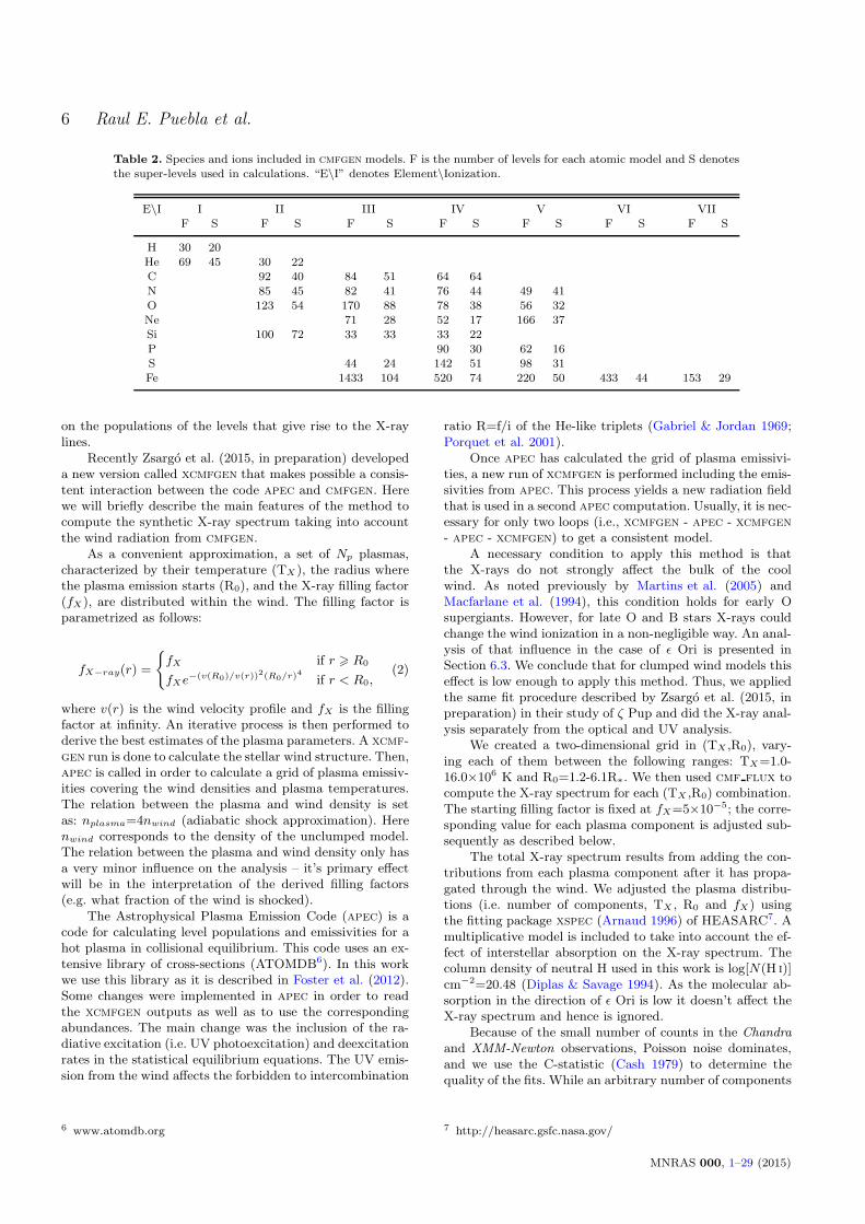
The calculations for our analysis were performed using thecode cmfgen (Hillier & Miller 1998). This code models aspherical stellar atmosphere and stellar wind solving the ra-diative transfer, radiative and statistical equilibrium equa-tion system in non-LTE (NLTE) taking into account line-blanketing effects. The transfer equation is solved in theco-moving frame (CMF). Table 2 describes the ionizationstates and number of full atomic levels and super-levels foreach atomic species included in the models.
The photospheric density structure is calculated by iter-atively solving the hydrostatic equilibrium equation systembelow the sonic point as described by Bouret et al. (2012).Given an adopted mass-loss rate and the velocity profilev(r), the wind density structure is calculated using the conti-nuity equation. The adopted velocity profile is similar to thatcommonly used for massive star winds (e.g. Hillier 2003):
v(r) =2vtr + (v∞ − 2vtr)(1− rtr/r)
β
1 + exp [(rtr − r)/heff ], (1)
where vtr and rtr are the transition velocity and radius,between the photosphere and wind. The transition point isset as the radius where v(rtr) = 0.75vs where vs∼15 kms−1
is the sound velocity. The term heff = vtr/(2(dv/dr)tr), isthe scale height, v∞ is the terminal velocity and β is theacceleration parameter.
Clumping is taken into account through the volume fill-ing factor f = ρ/ρ(r), where ρ is the homogeneous (un-clumped) wind density and ρ is the density in clumps. In thisapproach the clumps are assumed to be optically thin to ra-diation and the interclump medium is void (Hillier & Miller1999). The filling factor dependence with radius is definedby the relation: f = f∞ + (1 − f∞) exp(−v(r)/vcl), wherevcl characterizes the velocity where clumping starts.
It is well known that we need to include the effect of mi-croturbulence on the photospheric and wind spectrum (e.g.Howarth et al. 1997). For the formal solution, the depth de-pendence of the microturbulence velocity was parameterizedas in Hillier (2003): ξt = ξmin+(ξmax−ξmin)v(r)/v∞. Here,ξmin and ξmax are the photospheric and wind turbulencerespectively. In this work we varied the ξmin from 10 to20 kms−1, a reasonable range for early B supergiant stars(McErlean et al. 1998) and ξmax ∼ 0.1-0.3 v∞. In the CM-FGEN calculation we used a microturbulent velocity thatwas independent of depth.
4.1.2 X-ray Analysis
We assume that the X-ray emission comes from an ensembleof shock-heated regions within the wind (shock scenario).The shock scenario predicts regions distributed in the windwhere the plasma is strongly heated due to shocks caused byradiative instabilities (Owocki et al. 1988; Feldmeier et al.1997).
The current version of cmfgen allows for X-ray emis-sion from shocked regions in the wind using emissivity tablesfrom apec (Smith et al. 2001) for different temperatures,but it doesn’t take into account differences in abundances(generally), densities or the influence of the UV radiation
MNRAS 000, 1–29 (2015)
6 Raul E. Puebla et al.
Table 2. Species and ions included in cmfgen models. F is the number of levels for each atomic model and S denotesthe super-levels used in calculations. “E\I” denotes Element\Ionization.
E\I I II III IV V VI VIIF S F S F S F S F S F S F S
H 30 20He 69 45 30 22C 92 40 84 51 64 64N 85 45 82 41 76 44 49 41O 123 54 170 88 78 38 56 32Ne 71 28 52 17 166 37Si 100 72 33 33 33 22P 90 30 62 16S 44 24 142 51 98 31Fe 1433 104 520 74 220 50 433 44 153 29
on the populations of the levels that give rise to the X-raylines.
Recently Zsargo et al. (2015, in preparation) developeda new version called xcmfgen that makes possible a consis-tent interaction between the code apec and cmfgen. Herewe will briefly describe the main features of the method tocompute the synthetic X-ray spectrum taking into accountthe wind radiation from cmfgen.
As a convenient approximation, a set of Np plasmas,characterized by their temperature (TX ), the radius wherethe plasma emission starts (R0), and the X-ray filling factor(fX), are distributed within the wind. The filling factor isparametrized as follows:
fX−ray(r) =
{
fX if r > R0
fXe−(v(R0)/v(r))2(R0/r)
4
if r < R0,(2)
where v(r) is the wind velocity profile and fX is the fillingfactor at infinity. An iterative process is then performed toderive the best estimates of the plasma parameters. A xcmf-
gen run is done to calculate the stellar wind structure. Then,apec is called in order to calculate a grid of plasma emissiv-ities covering the wind densities and plasma temperatures.The relation between the plasma and wind density is setas: nplasma=4nwind (adiabatic shock approximation). Herenwind corresponds to the density of the unclumped model.The relation between the plasma and wind density only hasa very minor influence on the analysis – it’s primary effectwill be in the interpretation of the derived filling factors(e.g. what fraction of the wind is shocked).
The Astrophysical Plasma Emission Code (apec) is acode for calculating level populations and emissivities for ahot plasma in collisional equilibrium. This code uses an ex-tensive library of cross-sections (ATOMDB6). In this workwe use this library as it is described in Foster et al. (2012).Some changes were implemented in apec in order to readthe xcmfgen outputs as well as to use the correspondingabundances. The main change was the inclusion of the ra-diative excitation (i.e. UV photoexcitation) and deexcitationrates in the statistical equilibrium equations. The UV emis-sion from the wind affects the forbidden to intercombination
6 www.atomdb.org
ratio R=f/i of the He-like triplets (Gabriel & Jordan 1969;Porquet et al. 2001).
Once apec has calculated the grid of plasma emissivi-ties, a new run of xcmfgen is performed including the emis-sivities from apec. This process yields a new radiation fieldthat is used in a second apec computation. Usually, it is nec-essary for only two loops (i.e., xcmfgen - apec - xcmfgen- apec - xcmfgen) to get a consistent model.
A necessary condition to apply this method is thatthe X-rays do not strongly affect the bulk of the coolwind. As noted previously by Martins et al. (2005) andMacfarlane et al. (1994), this condition holds for early Osupergiants. However, for late O and B stars X-rays couldchange the wind ionization in a non-negligible way. An anal-ysis of that influence in the case of ǫ Ori is presented inSection 6.3. We conclude that for clumped wind models thiseffect is low enough to apply this method. Thus, we appliedthe same fit procedure described by Zsargo et al. (2015, inpreparation) in their study of ζ Pup and did the X-ray anal-ysis separately from the optical and UV analysis.
We created a two-dimensional grid in (TX ,R0), vary-ing each of them between the following ranges: TX=1.0-16.0×10⁶ K and R0=1.2-6.1R∗. We then used cmf flux tocompute the X-ray spectrum for each (TX ,R0) combination.The starting filling factor is fixed at fX=5×10⁻⁵; the corre-sponding value for each plasma component is adjusted sub-sequently as described below.
The total X-ray spectrum results from adding the con-tributions from each plasma component after it has propa-gated through the wind. We adjusted the plasma distribu-tions (i.e. number of components, TX , R0 and fX) usingthe fitting package xspec (Arnaud 1996) of HEASARC7. Amultiplicative model is included to take into account the ef-fect of interstellar absorption on the X-ray spectrum. Thecolumn density of neutral H used in this work is log[N(H i)]cm−2=20.48 (Diplas & Savage 1994). As the molecular ab-sorption in the direction of ǫ Ori is low it doesn’t affect theX-ray spectrum and hence is ignored.
Because of the small number of counts in the Chandraand XMM-Newton observations, Poisson noise dominates,and we use the C-statistic (Cash 1979) to determine thequality of the fits. While an arbitrary number of components
7 http://heasarc.gsfc.nasa.gov/
MNRAS 000, 1–29 (2015)

X-ray, UV and optical analysis of supergiants: ǫ Ori 7
Table 3. ǫ Ori Chandra and XMM-Newton lines. Data fromATOMDB.
Ion Wavelength (A) Type Tpeak [106 K]
Sixiv 6.1822 H-like 15.8Sixiii 6.6479, 6.6866, 6.6866 He-like 10.0Alxii 7.7573, 7.8070, 7.8721 He-like 7.94Mgxi 7.8503 He-like 6.31Mgxii 8.4210 H-like 10.0Mgxi 9.1687, 9.2297, 9.3143 He-like 6.31Nex 10.2388 H-like 6.31Ne ix 11.5440 He-like 3.98Nex 12.1339 H-like 6.31Fexvii 12.2660 L-shell 6.31Ne ix 13.4470, 13.5520, 13.6980 He-like 3.98Fexvii 14.2080 L-shell 7.94Fexvii 15.0140 L-shell 6.31Fexvii 15.2610 L-shell 6.31Fexvii 16.0040 L-shell 7.94Oviii 16.0060 H-like 3.16Fexvii 16.7800 L-shell 6.31Fexvii 17.0510 L-shell 6.31Fexvii 17.0960 L-shell 6.31Ovii 18.6270 He-like 2.00Oviii 18.9670 H-like 3.16Ovii 21.6020, 21.8040, 22.0980 He-like 2.00Nvii 24.7790 H-like 2.00Nvi 24.8980 He-like 1.59Cvi 26.9900 H-like 1.59Cvi 28.4650 H-like 1.59Nvi 28.7870, 29.0810, 29.5340 He-like 1.58Cvi 33.7370 H-like 1.26
can be included, the final models were typically composedof only four different temperatures.
The X-ray lines included in the analyses are listed inTable 3.
4.2 Stellar Parameters
We used the optical spectrum to estimate the photosphericparameters such as the effective temperature, gravity andsurface abundances. The method follows the analysis routedescribed by Bouret et al. (2012) (see also Martins et al.2005; Bouret et al. 2013). We adopted a radial velocityvr=25.9±0.9 km s−1 (Evans 1967).
A brief description of steps taken to derive the funda-mental stellar parameters (Teff , log g, and CNO, Fe and Siabundances) follows.
4.2.1 Luminosity
We adopt two distances: the distance d =411.5+245−112 pc
(Perryman et al. 1997) from the old HIPPARCOS catalog(HIP 26311)8, and d=606+227
−130 pc (van Leeuwen 2007) whoreanalyzed HIPPARCOS data. The errors on the distanceare approximately 30-50%, which will yield an error on theluminosity of 60-100%, and a similar, but somewhat smaller,uncertainty on the mass-loss rate.
A first estimation of luminosity was made based on
8 http://vizier.u-strasbg.fr/viz-bin/VizieR-2
MV and the bolometric correction (BC). The last onewas taken from the relation between Teff and BC calcu-lated by Crowther et al. (2006)(Fig. 4). This relation comesfrom their sample of Galactic B supergiants and from theSMC B supergiants reported by Trundle et al. (2004) andTrundle & Lennon (2005). For this first approach we usedthe temperature estimated by Crowther et al. for ǫ Ori,Teff=2.7×10⁴ K. The MV value was estimated from thedistance values from HIPPARCOS, the apparent visualmagnitude V=1.69 (Lee 1968) and the interstellar visualextinction AV =3.1 E(B-V), with E(B-V) taken from theCrowther et al. study, E(B-V)=0.06. Thus, MV =−6.57 ford=411.5 pc andMV =−7.41 for d=606.06 pc. The luminosityis given by:
log(L∗/L⊙) = (MB⊙ −MV −BC)/2.5, (3)
where MB⊙ is the solar bolometric magnitude (MB⊙=4.75).Once the temperature and gravity were estimated, we
used the UV flux, and the optical magnitudes (UV B) inorder to re-estimate simultaneously the luminosity and E(B-V) values.
4.2.2 Gravity and Effective Temperature
For estimating the effective temperature and gravity (log g)a small grid of models encompassing Teff=2.5-2.9×10⁴ Kand log g = 2.8 to 3.4, with steps of 0.1 × 10⁴ K and 0.1dex respectively, were computed. The gravity was estimatedby fitting the wings of Hβ, Hγ , Hδ and Hǫ – the lines wereequally weighted for the gravity analysis. Because of themass loss rate of ǫ Ori, these Balmer lines are only veryweakly influenced by wind emission. In order to reduce thedegeneracy between log g and Teff , the equivalent widths forHe i and He ii lines were also utilized. The lines used were:He i λλ4010, 4389, 5049 and He ii λλ4201, 4542. These linesshow a weak dependence on the microturbulence.
For computing the effective temperature we used theionization balance of both He i to He ii and Si iii to Si iv. Weused the same grid described above to fit the Si iv λ4090,Si iv λ4115 and Si iii λ4554-76 lines beside the He i λλ4471,4389, 4922 and the He ii lines described above. UV lines,especially those belonging to Fe iv (1550 - 1700 A), Fev(1360 - 1385 A) as well as Fe iii (1800-1950 A), were used tocheck the result.
4.2.3 Microturbulence
To estimate the photospheric microturbulent velocity wecalculated spectra for three values of ξmin (10, 15 and 20kms−1) and fitted the equivalent width of the 4472, 5017and 6680 A He i lines, and the Si iii triplet at 4554-4576 A.Our exploration of synthetic spectra shows that these linesdepend strongly on the ξmin value and are weakly influencedby blending or abundance effects.
4.2.4 Surface Abundances
Once the temperature and gravity were constrained, wedetermined the surface abundances of the main species,namely, He, C, N, O, Si and Fe as follows:
MNRAS 000, 1–29 (2015)

8 Raul E. Puebla et al.
Helium. As pointed out by McErlean et al. (1999, 1998),it is difficult to determine the He abundance in B stars pri-marily because triplet and singlet lines of He i yield differentHe abundances. Najarro et al. (2006) showed that some He isinglets are influenced by a strong interaction of the He iresonance transition at λλ4923,5017 with UV Fe iv lines.This interaction directly affects He i 2p 1Po, which influ-ences the strength of optical singlet lines that makes themunreliable diagnostics. Najarro et al. suggest using tripletlines for analysis. Based on these issues we decided to setthe He abundance, expressed as y = N [He]/N [He +H ], tothe solar value y=0.091 for every one of our models.Carbon. In the optical, we used lines of C ii λλ4267,6578-82,C iii λλ4070,5696,4648-50 and C iv λλ5802-12. In the case ofC iii λ4648 and C iii λ5696, Martins & Hillier (2012) showedthat these lines have strong interactions with the UV linesFe iv λ538 and C iii λ538, hence, they need be treated care-fully. UV lines were used to check the abundance deducedfrom optical lines. We mainly used C iii λ1176. The com-monly used line C iv λ1169 is not detected in UV data, sinceit is blended with C iii λ1176. The line C iii λ1247 is blendedwith Nv λ1238-42 emission and only the red emission canbe used as a diagnostic.Nitrogen. To estimate the nitrogen abundance we usedthe blend-free lines N ii λλ3995, 4042-45, 4238-42, 5002-06,5677-81, and N iii λλ4380, 4635. As a consistency check wealso examined N ii λ5046 and N iii λλ4098, 4512-18, 4643,4868. The former line is blended with He i λ5049 while N iii
λ4098 is blended with Hδ. In the UV we used N iii λλ1183-85 and N iii λλ1748-52. The N iv λ1718 line was excludedbecause it is affected by the wind and Nv λ1240 is X-raysensitive, and hence not suitable as an abundance diagnos-tic.Oxygen. ǫ Ori shows a variety of O ii and O iii lines — ourabundance analysis was based on: O iii λλ4368, 5594 andO ii λλ4077, 4134, 4663. Other lines that show abundancedependence are those in the blend O ii-iii λ4415-18. TheUV lines commonly used for abundance diagnostics are O iv
λλ1338-43 and O iii λλ1150-54 but they show only a weakabundance dependence in the models. Ov λ1371 was notdetected in the UV spectra of ǫ Ori.Silicon. The silicon abundance was estimated using onlySi iii and Si iv lines since Si ii lines were not detected. Thetriplet Si iii λλ4552-67-74 and Si iii λ5738 were useful as wellas Si iv λλ4089, 4116. No UV lines were used for the analysisdue to their strong dependence on the wind parameters.Iron. We only used UV Fe lines for estimating its abun-dance. The iron features Fev λλ1360 - 1385, Fe iv λλ1550 -1700, and Fe iii λ1800-1950 were used. Again, it is importantto have a reliable value for temperature to get an accurateabundance estimation.
4.2.5 Rotation and Macroturbulence
We account for the influence of rotation on the stellar spec-trum in two ways. First, we convolve a rotational broadeningprofile with the synthetic spectrum. This method assumessolid rotation of both the star and wind, and that the lineprofile does not vary from the center to the limb (Gray 2008).Wind-free line profiles were used to estimate the projectedrotation velocity (vrot sin i).
In the second technique we calculate the synthetic spec-
trum using the 2D code developed by Busche & Hillier(2005). This code computes the radiative transfer throughthe photosphere and wind using an axysimmetric geometryand allows for rotation of the star. Recently, Hillier et al.(2012) studied the application of the code to optical lineprofiles of O stars. They showed that while the convolu-tion method that is commonly used to allow for rotation isadequate for photospheric absorption lines it fails for linesinfluenced by photospheric emission, or for lines with windemission contribution. For the diagnostic lines Hα and He iiλ4686 it is important that the influence of rotation be cor-rectly modeled.
Because the rotation rate of ǫ Ori is low we can use thesame simplifications as Hillier et al. (2012) – we assume therotation does not affect the density structure, temperatureand surface gravity. We also assume that the star rotatesas a solid body below v(r)=20 kms−1 and the angular mo-mentum about the center is conserved above that value.
Finally, in order to compare the synthetic spectra withthe optical observational data, it is necessary to take intoaccount instrumental broadening and macroturbulence. In-strumental broadening was taken into account by convolvinga Gaussian profile of 4.0 kms−1 from NARVAL spectral res-olution. Macroturbulence broadening was included througha convolution assuming an isotropic Gaussian distributedvelocity field. The value of the FWMH of such a distribu-tion in km s−1 was estimated using the wings of isolatedwind-free metallic lines.
4.3 Wind Parameters
The parameters that describe the stellar wind are those thathave to do with the wind velocity law (β and v∞), the mass-loss rate (M), the filling factor (f∞, vcl) and the wind turbu-lent velocity (ξmax). All of these influence spectral featuresin the UV, optical, and X-ray band. Some line profiles arestrongly influenced by two or more of the parameters. Forexample, the strength of Hα is highly sensitive to both themass-loss rate and filling factor, and its profile shape is sen-sitive to β. Thus, these wind parameters need to be deter-mined simultaneously using several spectral features fromdifferent ions and species.
The value of M is first constrained using the Hαstrength for f∞= 1.0, 0.1, 0.05 and 0.01 (f∞=1.0 meanssmooth wind). A consistency check was then done usingthe UV line profiles of C iv λλ1548,1551, Nv λ1240, Si ivλλ1394,1403 and C iii λ1776, which showed only a weak de-pendence on mass-loss rate (in our models) when comparedwith Hα.
The clumping factor (f∞) is determined using S ivλλ1062,1073, Pv λλ1118-28 and N iv λ1718. The param-eter vcl has a slight influence on the Hα shape, so its valueis adjusted only to improve the line profile once the M is es-timated from line strength. Hillier (2003) suggested that itsvalue should be less than 100 kms−1. Likewise, Bouret et al.(2003) (see also Bouret et al. 2005) suggested that clumpingshould start close to the photosphere (vcl ∼30 kms−1). Forthe models in this work, we used vcl values from 20 to 100kms−1.
The velocity profile parameters (v∞, β) were con-strained using UV P Cygni line profiles and the Hα lineprofile. The Hα profile shape is strongly sensitive to β – we
MNRAS 000, 1–29 (2015)

X-ray, UV and optical analysis of supergiants: ǫ Ori 9
used values from 1.0 to 2.4 to find the best profile. Once wealter β it is necessary to re-tune the mass-loss rate to matchthe Hα intensity.
In the same sense, v∞ was estimated using the bluewing of the P Cyg profile of C iv λλ1548,1551 and the Si ivλλ1394,1403 profile. As the shape of that wing is also af-fected by the wind turbulence ξmax we tune v∞ and ξmax
simultaneously.
4.4 X-ray – Wind Parameters
As X-rays propagate through the wind they can be absorbedat the same time photoionize the gas. The effect on an X-rayline is an attenuation of the profile on the red side, becausethe red-shifted photons from the rear hemisphere encountera longer path length through the wind than the blue-shiftedphotons from the front hemisphere (Owocki & Cohen 2001;Macfarlane et al. 1991). Since the X-ray opacity varies withwavelength the influence on line profiles varies with wave-length. Furthermore, the strength of the effect depends pri-marily on the wind column density and hence the mass-lossrate. Thus, with a known opacity distribution, it is possibleto estimate the mass-loss rate from the observed X-ray lines(Cohen et al. 2014a).
In this work we utilize X-ray cross-sections fromVerner & Yakovlev (1995). The spatial variation in opac-ity is determined by the velocity law and mass-loss rate.We use the same values estimated from the optical andUV data. Once the best fit is attained, the line profilesare checked for consistency. Previous M estimations from X-ray lines used individual line profiles (Oskinova et al. 2006;Cohen et al. 2014a); in this work we use models for the wholeX-ray spectrum. A similar approximation was developed byHerve et al. (2013), but they used a fiducial radial depen-dence for opacity.
The effects of v∞ and β on X-ray profiles have beenstudied by Cohen et al. (2010). Here, we use the same val-ues obtained from the optical and UV analysis. We showbelow that β can influence R0, and this gives us the op-portunity to check our results against the instability windmodels (Feldmeier et al. 1997; Runacres & Owocki 2002;Dessart & Owocki 2003, 2005) relating the wind accelera-tion with the shock formation region.
4.5 X-ray – Abundances
Once global best fit to the X-ray spectra is obtained, theabundances are adjusted so as to improve the fit of lineratios.
To compute the observed line strength ratios, the linefluxes were measured using Gaussian profiles and the sta-tistical tools from xspec. The free parameters for each fitwere the normalization factor and the line width (σ of eachGaussian). The line center is generally fixed at its labora-tory value, but when necessary it was shifted to match thepeak of the observed line – it was not included as a freeparameter in the fit. We will specifically focus on the CNO
line ratios. Recently Zsargo et al. (in preparation) showedthat good choices are:
R(N/O) =F lux(Nvii Lyα)
[F lux(Oviii Lyα) + F lux(Ovii He− Like)],
(4)and
R(C/N) =F lux(Cvi Lyα)
[F lux(Nvii Lyα) + F lux(Nvi He− Like)],
(5)that have a weak dependence on temperature and are goodchoices to test the consistency of our abundance values fromthe optical and UV analysis. New abundances can be esti-mated when the observed ratios are compared with the onesfrom our models.
5 RESULTS
5.1 Stellar Parameters
The main stellar parameters that we estimated for ǫ Oriare shown in Table 4. Each row in the table corre-sponds to the parameters from the two different dis-tances from the HIPPARCOS catalogs. The luminosityfrom the lower distance lies between those calculated byCrowther et al. (2006) (log(L∗/L⊙)=5.44) and Searle et al.(2008) (log(L∗/L⊙)=5.73) and is close to other estimates re-ported in the literature (e.g. Lamers 1974; Kudritzki et al.1999; McErlean et al. 1999). The luminosity computed withthe larger distance is the highest value reported and makesǫ Ori one of the most luminous B-supergiants in the Galaxy.This value is almost twice the calibrated value found bySearle et al. (2008) for galactic B0Ia stars (They used jointlytheir sample and that of Crowther et al. (2006).). A sim-ilar statement applies to the mass-loss rate and stellar ra-dius (mass). Thus the distance of van Leeuwen (2007) makesǫ Ori an unusual B0Ia supergiant. For the analysis, we preferto use the lower value in order to compare with the previouswork on ǫ Ori that were undertaken assuming a distancecloser to that of Perryman et al..
Figure 1 shows the analysis of Balmer line wings andHe i-ii lines. We concluded that log g=3.0. We also foundthat for values greater than 3.05 and lower than 2.95 it isnot possible to fit the Balmer and He i-ii lines consistently.Thus, we estimate an error of 0.05 for log g.
Figure 2 shows the analysis for the ionization balanceof He i-ii and Si iii-iv. The ionization balance of He i-iiyields an effective temperature approximately 2.65 × 10⁴
to 2.68 × 10⁴ K while the Si iii-iv ionization balance yieldsa value ∼ 2.68 × 10⁴ to 2.75 × 10⁴ K. From these resultswe concluded that the effective temperature of ǫ Ori isTeff=27000±500K. In the UV, Si iii λ1312 shows a strongdependence on temperature. This line yields a slightly lowertemperature of Teff=26200 K. Nevertheless, Fe iv-v linesand the O iv λλ1342,1343 lines support a value of 27000 K.The Si iii-iv λλ1417,1416 lines provide a temperature esti-mate of 27500 K.
Photospheric microturbulence velocity (ξmin) was es-timated to be between 15 and 20 km s−1 using He i lines.The silicon triplet (4554-4576 A) suggests a ξmin close to
MNRAS 000, 1–29 (2015)

10 Raul E. Puebla et al.
Table 4. Stellar parameters of ǫ Ori from optical and UV data.
Log (L∗/L⊙)d Teff log g R∗ M∗ ξmin v sin i vmacro E(B-V) d103 [K] R⊙ M⊙ km s−1 km s−1 km s−1 mag pc
5.59+0.51−0.20 27.0±0.5 3.0±0.05 28.6 30.0 15-20 40-70c 70-100 0.091 ± 0.01 412a
5.92+0.32−0.18 27.0±0.5 3.0±0.05 42.0 64.5 15-20 40-70c 70-100 0.091 ± 0.01 606b
a HIPPARCOS catalog (Perryman et al. 1997)b HIPPARCOS catalog (van Leeuwen 2007)c Value computed using the convolution method.d Errors from distance uncertainties.
Table 5. Wind parameters of ǫ Ori from optical and UV data. The mass-loss rate forboth HIPPARCOS distances is given.
Model f∞ M/√f∞a M/
√f∞b v∞ β ξmax vcl
M⊙ yr−1 M⊙ yr−1 kms−1 km s−1 kms−1
A 0.1 1.55×10⁻⁶ 2.70×10⁻⁶ 1800 2.0 200 40B 0.05 1.66×10⁻⁶ 2.80×10⁻⁶ 1800 2.0 200 30C 0.01 1.75×10⁻⁶ 2.90×10⁻⁶ 1800 2.0 200 20D 1.0 1.40×10⁻⁶ 2.55×10⁻⁶ 1800 2.0 200 –
a HIPPARCOS catalog (Perryman et al. 1997) (d=412 pc)b HIPPARCOS catalog (van Leeuwen 2007) (d=606 pc)
25 26 27 28 29
Teff
103[K]
2.7
2.8
2.9
3
3.1
3.2
3.3
log (
g)
Hε,δ,γ,β
He I 4010,4389,5049
He II 4201, 4542
Figure 1. Constraints on Teff and log g. Shown are fits to theBalmer line wings (black), the equivalent width of He i (red) andHe ii (blue) lines.
the lower limit, 15 km s−1 while the UV Si iii multiplet in-dicates a microturbulence closer to 10 kms−1(Fig. 3). Thevariations do not change the reported limits for temperatureand gravity.
Figure 3 shows the line profiles for optical and UV Si iiilines. The models correspond to three values of turbulencevelocity: 20 km s−1 (red), 10 km s−1 (blue) and 5 km s−1
(green). We found divergence between the UV and opticalsilicon lines – the UV (Si iii λλ1290-1310) complex suggestsξmin ∼10 kms−1 while the optical triplet Si iii λλ4550-4580 requires a value of ξmin ∼20 kms−1. Furthermore,
the Fe iv λλ1450-1500 and Fe iv λλ1600 -1700 lines rule outξmin lower than ∼10 kms−1.
The discrepancy between UV and optical Si iii lines canbe overcome by increasing the silicon abundance by a fac-tor of ∼1.2 with ξmin=15 kms−1. However, such a value isincompatible with other optical lines (e.g. N iii λ4098 andC iii λλ4648-4654).
The rotation and macroturbulence velocities were es-timated simultaneously from fitting the line shapes. Weestimated values of 40-70 kms−1 for rotation and 70-100kms−1 for vmacro. That rotation value is lower than pre-viously reported (v sin i = 91 km s−1 by Howarth et al.(1997)). However upon close examination we found this ro-tation rate accurately fits some optical line profiles, such asthose belonging to Si iii λ4554-4576. Rotation is analyzed in§ 5.7.
5.2 Wind Parameters
We calculated models for four different values of filling factor(f∞). The best fitting parameters for each of these modelsare shown in the Table 5. We use capital letters as referencefor the subsequent analysis. The best synthetic spectra foreach filling factor from UV to optical together with data areshown in Appendix A.
5.2.1 Mass-loss rate
Because of the strong sensitivity of the Hα line profile tothe mass-loss rate, it is possible to attain high precision forthis parameter through fitting its line strength. We foundM/
√f∞≈1.6×10⁻⁶ M⊙ yr−1 for ǫ Ori (d=412 pc). The
mass-loss rate for each filling factor is shown in Table 5.As expected, M/
√f∞ is almost independent of f∞, and
is lower than the value M∼2×10⁻⁶ M⊙ yr−1estimated bySearle et al. (2008) and Crowther et al. (2006). The main
MNRAS 000, 1–29 (2015)

X-ray, UV and optical analysis of supergiants: ǫ Ori 11
25.5 26 26.5 27 27.5 28Teff [103 K]
0.05
0.1
0.15
0.2
EW
(He
II)/
EW
(He
I)
He II 4200 / He I 4471He II 4542 / He I 4471
25.5 26 26.5 27 27.5 28Teff [103 K]
0
5
10
15
EW
(Si I
V)/
EW
(Si I
II)
Si IV 4090 / Si III 4576Si IV 4115/ Si III 4576
25.5 26 26.5 27 27.5 28Teff [103 K]
0
0.2
0.4
0.6
0.8
EW
(He
II)/
EW
(He
I)
He II 4200 / He I 4387He II 4200 / He I 4922He II 4542 / He I 4387He II 4542 / He I 4922
25.5 26 26.5 27 27.5 28Teff [103 K]
1
2
3
4
EW
(Si I
V)/
EW
(Si I
II)
Si IV 4090 / Si III 4554Si IV 4090 / Si III 4569Si IV 4115 / Si III 4554Si IV 4115 / Si III 4569
Figure 2. Ionization balance for He i-ii and Si iii-iv. The ratio of equivalent widths (EWs) for selected pairs of He and Si lines areshown for models with log g=3.0 and Teff =2.55-2.8×10⁴ K. Each square represents the model that matches the observed ratio of theequivalent widths (EWs) of the lines. The horizontal dashed lines show the equivalent width ratios measured from optical data, whilethe vertical dashed lines show the projection of the matching model EW to the temperature axis. We estimated the measured EW ratioerrors. The maximum is around 1 %, which would influence our lower temperature limit by .100 K.
Figure 3. Dependence of UV and optical Si iii lines on photospheric microturbulence (ξmin). In the left panel, the black line representsthe GHRS data and the gray line COPERNICUS data. Profiles for three photospheric microturbulent velocities are shown: 20 km s−1
(red), 10 km s−1 (blue) and 5 km s−1 (green).
MNRAS 000, 1–29 (2015)

12 Raul E. Puebla et al.
reason for the discrepancy is their adopted lower values forβ (1.1 and 1.5, respectively). A lower β value yields lowerdensities in the Hα formation region, and hence a highermass-loss rate is required to fit the line emission. As thesevalues were computed using mainly Hα, its variability willincrease the uncertainty of the mass-loss rate. Morel et al.(2004) and Thompson & Morrison (2013) reported Hα vari-ability in its shape profile and strength. The results shownhere are based on data collected on a specific date, anddon’t show Hα variability during observations. We changedthe mass-loss rate in order to obtain the strongest and theweakest line from Thompson & Morrison’s profile. The cor-responding values are 4.8×10⁻⁷ and 2.8×10⁻⁷ M⊙ yr−1 re-spectively (assuming β = 2, f∞ = 0.05 and d = 412 pc). Thevariation is approximately 30% about our derived mass-lossrate of 3.6×10⁻⁷ M⊙ yr−1. This shows that small changeson M yield larges changes in the Hα profile. A full variabilityanalysis is necessary to improve our conclusions about M forǫ Ori, but this kind of analysis is beyond the scope of thispaper.
In our analysis we did not include the infrared (IR) andradio spectral regions, but we can compare our results withthose from previous studies. Blomme et al. (2002) used radiofluxes from 3.6 and 6.0 cm and computed a M∼1.66×10⁻⁶
M⊙ yr−1 assuming a smooth model. This is consistent withour estimate, but only if clumping persists into the radio re-gion (our model fluxes at 6.0 cm is ∼0.7 mJy, while the meanof reported Blomme et al.’s ones is∼0.74±0.13. mJy.). Mod-els by Runacres & Owocki (2002) indicate that structure canpersist into the radio region and may influence radio diag-nostics. On the other hand Puls et al. (2006) found a differ-ence between stars with strong and weak winds. For strongwinds their analysis suggested that wind clumping declinedinto the radio region while for weak winds they found sim-ilar clumping in the inner and outer wind. In future workradio and millimeter fluxes should be incorporated into theanalysis.
Using IR observations Repolust et al. (2005) obtainedM/
√f∞=3.7×10⁻⁶ M⊙ yr−1 while Najarro et al. (2011) de-
rived M/√f∞=2.0×10−6 M⊙ yr−1 (for the comparisons we
scaled the reported values to our distance and v∞). TheM derived by Najarro et al. is consistent with our estimatewhile that of Repolust et al. is a factor of ∼ 2 higher.
UV lines are less sensitive than Hα to changes inM/
√f∞. Therefore, we use UV lines only to confirm our
Hα values. Moreover, UV line strengths also depend on ion-ization structure and some of them also on the X-ray emis-sion (e.g. Nv and C iv). The X-ray independent and non-saturated UV line C iii λ1176 confirmed the M(Hα) values.Si iv λλ1394-1402 was not well reproduced, likely because ofvorosity-porosity effects, so it was disregarded in the analy-sis (§ 6).
5.2.2 Velocity profile
The wind acceleration parameter (β) strongly affects the Hαprofile (Hillier 2003). The Hα profiles calculated for β=1.0,1.5 2.0 and 2.2 are shown in Figure 4. From this figure,we concluded that the better β value is around 2.0 (valueslower that 1.8 or higher that 2.2 were unable to reproducethe profile). This value is higher than others previously cal-culated for early B-supergiants (e.g. Kudritzki et al. 1999;
Figure 4. Hα profiles for different β values: 1.0 (green), 1.5 (pur-ple), 2.0 (red) and 2.5 (blue). Black line represents the optical
data. Each line profile was computed with the M that matchesthe observed line strength.
Crowther et al. 2006; Searle et al. 2008). For each β we ex-plored a wide range for M/
√f∞, however we were unable to
match the observed line profile for low β values.Crowther et al. (β=1.5) used two sets of optical data
for ǫ Ori, but the line shape was not reproduced in eithercase. They obtained high velocity wing emission that is notdetected, and they were unable to reproduce the blue ab-sorption observed in Hα profile.
Searle et al. (β=1.1) do not show their Hα profile; wetried to fit this line with their β value by tuning other windparameters but we were unable to reproduce the line shapewith such a low β value.
In the above works other Galactic early-type B-supergiant stars were also analyzed. The derived β valuesare between 1.0 and 1.5. For Small Magellanic Cloud (SMC)B0-B1 supergiants, Trundle et al. (2004) also found β valueslower than ours. Evans et al. (2004) analyzed two B0Ia starswithin a sample of supergiants from the Magellanic Clouds:AV235 and HDE 269050. They found β parameters of 2.50and 2.75, respectively.
Spectral variability of Hα could be one reason for thediscrepancy between our values and those derived from pre-vious works. Thompson & Morrison (2013) reported profilevariability on a time scale of weeks. This variability is stillnot understood (see also Martins et al. 2015). An alterna-tive to be investigated in the future is a different radial de-pendence for the filling factor. Runacres & Owocki (2002)predicted that the clumping factor (fcl = 1/f) grows until10-50 R∗ and then falls in the outer wind regions. However,Puls et al. (2006) shows that for denser winds high clumpingfactors are present close to the stellar surface. ǫ Ori doesn’tshow a high mass-loss rate, but a different clumping distri-bution should be investigated in combination with other βvalues.
The v∞ and ξmax parameters were estimated togetherusing the blue absorption wing of UV lines, especially C iv
MNRAS 000, 1–29 (2015)

X-ray, UV and optical analysis of supergiants: ǫ Ori 13
λ1550 and C iii λ1175. We found that the value of v∞ liesbetween 1700 and 1800 kms−1, while the wind turbulencevelocity is ξmax∼200 kms−1.
The values calculated here are between the previousones calculated by Crowther et al. (2006) and Searle et al.(2008) (1600 and 1910 km s−1 respectively). The C iii λ1175profile rules out a value of 1600 kms−1 for v∞, since a valueof ξmax &300 kms−1 is necessary in order to fit the blue ab-sorption wing. Such a high value for ξmax distorts the Si ivλ1400 profile and the C iv λ1550 blue absorption wing.
5.2.3 Clumping
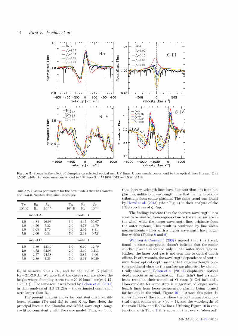
Besides the mass-loss rate, we also changed vcl (the pointwhere the clumping starts) aiming to optimize the Hα pro-file. The best values for vcl for each f∞ are shown in Table 5and are between 20 and 40 km s−1. Figure 5 shows the effectof f∞ on different lines in the optical and UV. We found thatS iv λλ1062,1073 and N iv λ1718 yield a low value for f∞(60.01). The same was found for Pv λλ1118-28 (not shownin the figure). On the other hand, the optical lines yield amoderate value between 0.05 and 0.1. These discrepanciescannot be corrected by altering the mass-loss rates withoutspoiling the Hα profile. It is possible to alter the abundancesuntil the model fits the lines, but the derived values for a rea-sonable value for f∞ are too low to be plausible, especiallyfor sulfur.
5.3 Abundances from UV and Optical
We chose model “A” to estimate the abundances of CNO, Siand Fe. The lines selected for estimating the abundances arenot affected by wind emission, hence it is irrelevant whichmodel, from Table 5, we choose. Solar abundances for Si andFe fit the optical and UV spectra to within 10%. Becauseof this, we fixed their abundances to solar values and con-centrated our analysis on CNO abundances. Nevertheless,as it was noted above, a silicon abundance of 1.2 Si⊙ helpsto reconcile the fit to the UV and optical Si iii multiplets.
Figure 6 shows three panels. In each of these panels they-axis shows the abundance estimate obtained from eachtransition and the x-axis shows the line wavelength. Thenumerical abundances are relative to hydrogen, expressedas: log(NX/NH) + 12. The filled black line represents themean value (simple average) while the dashed lines representthe standard deviation of those measurements.
Table 6 shows the mean CNO abundances and theirstandard deviations, the N/C and N/O abundance ratios,and the corresponding solar values. These ratios are calcu-lated as: [N/(C,O)]= log(NN/N(C,O))∗ − log(NN/N(C,O))⊙.The other three columns show previous abundance estimatesfrom Crowther et al. (C06) and Searle et al. (S08).
Our values for [N/(C,O)] show a small nitrogen en-hancement and carbon and oxygen depletion. This providesevidence for CNO processed material at the star surface.Nevertheless, when compared with C06 and S08, our valuesare closer to the solar ones.
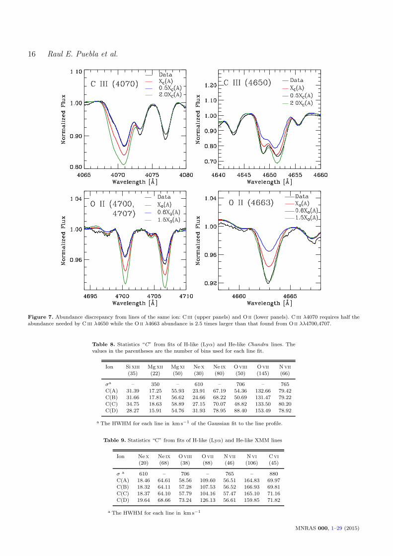
The abundance determinations typically scatter withina factor of 2 either side of the mean, as shown in Figure 6.Figure 7 shows the sensitivity of several lines to the abun-dance. For instance, C iii λ4070 requires half of the abun-dance predicted by C iii λ4650. Similarly the O ii λλ4663
Table 6. CNO abundances from optical and UV data.[N/C,O]=log(NN/NC,O)∗ − log(NN /NC,O)⊙
Species This Work σ(dex) S08 C06 Solar
C 8.16 0.16 7.66 7.95 8.43N 7.90 0.18 7.31 8.15 7.83O 8.58 0.17 8.68 8.55 8.69Si 7.51 0.04 7.51 7.51 7.51Fe 7.50 0.04 7.50 7.50 7.50
[N/C] +0.33 – +0.26 +0.8 0.00[N/O] +0.15 – -0.49 +0.5 0.00
abundance is 2.5 times larger than that obtained with O ii
λλ4700,4707.The possible causes of the abundance discrepancies
are many — complex NLTE effects, deficiencies in theatomic models, blending, issues related to microturbulenceand macroturbulence. For example, it was pointed out byNieva & Przybilla (2006) that NLTE effects can cause dis-crepancy between the abundances estimated using C ii lines4267 A and 6587-82 A. We didn’t find strong discrepanciesamong these lines — the difference is not larger than 0.2 dex.Likewise, complex NLTE effects could affect the abundanceestimates of other lines such as C iii (Martins & Hillier 2012)and N ii-iv (Rivero Gonzalez et al. 2011, 2012b,a).
5.4 Wind Parameters from X-rays
We performed the fit procedure as described in Section 4.1.2,using the Chandra and XMM-Newton data simultaneously.The results for each of the models described above (A, B,C and D) are shown in Table 7. For each model we foundthat low temperature (∼1-3×10⁶ K) plasmas are necessaryto account for the Nvii Lyα, Nvi Heα and Cvi Lyα lines, aswell as the He-like line of Ne ix Heα. Similarily, a hot compo-nent is needed to account for Sixiii, Mgxii and Mgxi lines.The Sixiv Lyα at 6.18 A is not detected by Chandra, andhence the hottest plasma temperature is less than 1×10⁷ K.These temperatures are consistent with the distribution ofheating-rates computed by Cohen et al. (2014b) for ǫ Ori.They show that ǫ Ori has low heating rates for T&107 K.
Figures 8 and 9 show the Chandra and XMM-Newtondata with the models A (green), B (blue), C (orange) andD(red), respectively. The fits are reasonable for most lines,except for Nex λ12.13 which is too weak in all our mod-els. The fit of this line is strongly coupled to the fitting ofthe Mgxi-xii lines — better Nex line profiles were obtainedwhen those lines were excluded from the fits but the modelMg lines are too strong. The whole fit improves if we lowerthe Mg abundance approximately 10%. On the other hand,Drake & Testa (2005) and Cunha et al. (2006) have sug-gested that the currently accepted solar abundance of neonmight be underestimated. We computed models increasingthe Ne abundance by 40%, although the Nex λ12.13 profilesimprove, the emission in the Ne He-like triplet is overesti-mated.
Table 7 shows the spatial distribution of the emittingplasmas. Typically the coolest plasma is found to exist atlarger radii than the hottest plasma. Specifically, for 106 Kplasma R0 is around 4-4.9 R∗, for the 2-3×10⁶ K plasma
MNRAS 000, 1–29 (2015)
14 Raul E. Puebla et al.
Figure 5. Shown is the effect of clumping on selected optical and UV lines. Upper panels correspond to the optical lines Hα and C iii
λ5697, while the lower ones correspond to UV lines S iv λλ1062,1073 and N iv λ1718.
Table 7. Plasma parameters for the best models that fit Chandraand XMM-Newton data simultaneously.
TX R0 fX TX R0 fX106 K R∗ 10−3 106 K R∗ 10−3
model A model B
1.0 4.84 26.93 1.0 4.45 50.672.0 4.56 7.22 2.0 4.73 14.703.0 3.05 4.76 3.0 2.95 8.317.0 2.60 0.34 7.0 2.63 0.72
model C model D
1.0 3.89 123.0 1.0 6.10 12.792.0 4.72 62.03 2.0 3.40 1.1113.0 2.77 24.58 3.0 3.85 1.667.0 2.89 4.26 7.0 2.14 0.029
R0 is between ∼3-4.7 R∗, and for the 7×10⁶ K plasmaR0 ∼2.1-2.9 R∗. We note that the onset radii are above theheight where clumping starts (vcl=20-40 kms−1=v(r∼1.12-1.23 R∗)). The same result was found by Cohen et al. (2011)in their analysis of HD 93129A – the estimated onset radiiwere larger than Rcl.
The present analysis allows for contributions from dif-ferent plasmas (TX and R0) to each X-ray line. Here, theprincipal lines in the Chandra and XMM wavelength rangeare fitted consistently with the same model. Thus, we found
that short wavelength lines have flux contributions from hotplasmas, unlike long wavelength lines that mainly have con-tributions from colder plasmas. The same trend was foundby Herve et al. (2013) (their Fig. 4) in their analysis of theRGS spectrum of ζ Pup.
The findings indicate that the shortest wavelength linesstart to be emitted from regions close to the stellar surface inthe wind, while the longer wavelength lines originate fromthe outer regions. This result is confirmed by line widthmeasurements – lines with a higher wavelength have largerline widths (Tables 8 and 9).
Waldron & Cassinelli (2007) argued that this trend,found in some supergiants, doesn’t indicate that the coolershocked plasma is formed only in the outer wind regions.Rather, the inner cool gas is not seen due to optical deptheffects. In other words, the wavelength dependence of contin-uum X-ray optical depth means that long-wavelength pho-tons produced close to the surface are absorbed by the op-tically thick wind. Cohen et al. (2014a) emphasized opticaldepth effects as an explanation. They didn’t find a signif-icant trend in their sample of O stars (ǫ Ori included).However data for some stars is suggestive of longer wave-length lines from lower-temperature plasma being formedfarther out in the wind. Figure 10 illustrates this point. Itshows curves of the radius where the continuum X-ray op-tical depth equals unity, r(τx = 1), and the wavelengths ofthe main H-like and He-like lines. Utilizing Figure 10 in con-junction with Table 7 it is apparent that every “observed”
MNRAS 000, 1–29 (2015)

X-ray, UV and optical analysis of supergiants: ǫ Ori 15
4000 4500 5000 5500 6000 6500 7000Wavelenght (A)
7.8
7.9
8
8.1
8.2
8.3
8.4
Log
(NC/N
H)+
12
C II linesC III linesC IV lines
3000 3500 4000 4500 5000 5500 6000Wavelenght (A)
7.5
7.6
7.7
7.8
7.9
8
8.1
8.2
Log
(NN
/NH
)+12
N III linesN II Lines
4000 4500 5000 5500Wavelenght (A)
8.3
8.4
8.5
8.6
8.7
8.8
8.9
Log
(NO
/NH
)+12
O II linesO III lines
Figure 6. Abundances for CNO. The dots show the abundance that fits each line for each ion and species. The black line is the meanof those abundances, the dashed lines are the mean ± the standard deviation and the filled blue line represents the solar value.
plasma exists above the r(τx=1) where the transmissionfactor is high for each wavelength, as was pointed out byLeutenegger et al. (2010). Despite the high R0, we estimatethat ∼ 70% of the emitted X-rays are absorbed by the wind– the X-ray absorption is very signifcant for λ &12 A.
Figures 11 and 12 show the calculated line profiles forsome H-like and He-like X-ray lines together with data fromChandra and XMM. H-like profiles are centered at the redcomponent of the doublet, whilst He-like profiles are cen-tered at the red component of the intercombination dou-
blet. A visual inspection shows that the observed lines areslightly blue-shifted, and that every model reasonably re-produces the profiles, with the exception of model “D” (redline). This is especially clear when we look at the Oviii
profile.
In order to clarify which models match the observationswe calculated the “C” statistics for each H-line and He-likeline model profile. To do this we allow the flux for eachmodel profile to be a free-parameter, and choose the scal-ing that minimizes the C statistic. The results are shown
MNRAS 000, 1–29 (2015)
16 Raul E. Puebla et al.
Figure 7. Abundance discrepancy from lines of the same ion: C iii (upper panels) and O ii (lower panels). C iii λ4070 requires half theabundance needed by C iii λ4650 while the O ii λ4663 abundance is 2.5 times larger than that found from O ii λλ4700,4707.
Table 8. Statistics “C” from fits of H-like (Lyα) and He-like Chandra lines. Thevalues in the parentheses are the number of bins used for each line fit.
Ion Si xiii Mgxii Mgxi Nex Ne ix Oviii Ovii Nvii
(35) (22) (50) (30) (80) (50) (145) (66)
σa – 350 – 610 – 706 – 765C(A) 31.39 17.25 55.93 23.91 67.19 54.36 132.66 79.42C(B) 31.66 17.81 56.62 24.66 68.22 50.69 131.47 79.22C(C) 34.75 18.63 58.89 27.15 70.07 48.82 133.50 80.20C(D) 28.27 15.91 54.76 31.93 78.95 88.40 153.49 78.92
a The HWHM for each line in km s−1 of the Gaussian fit to the line profile.
Table 9. Statistics “C” from fits of H-like (Lyα) and He-like XMM lines
Ion Nex Ne ix Oviii Ovii Nvii Nvi Cvi
(20) (68) (38) (88) (46) (106) (45)
σ a 610 – 706 – 765 – 880C(A) 18.46 64.61 58.56 109.60 56.51 164.83 69.97C(B) 18.32 64.11 57.28 107.53 56.52 166.93 69.81C(C) 18.37 64.10 57.79 104.16 57.47 165.10 71.16C(D) 19.64 68.66 73.24 126.13 56.61 159.85 71.82
a The HWHM for each line in km s−1
MNRAS 000, 1–29 (2015)

X-ray, UV and optical analysis of supergiants: ǫ Ori 17
Figure 8. Chandra data (gray squares with error bars) and best X-ray models for A(green), B(blue), C(orange), and D(red). Dots linesshow the K-shell ionization threshold for O iii and O iv. The models are indistinguishable except for a few lines.
in Tables 8 and 9 for Chandra and XMM data respectively.From the values, we confirm that the smooth wind model(model “D”) can be ruled out based on the fit to Oviii andOvii (∆C≫6.63 when compared to the minimum amongthe other values of the same line), although the Ne ix, Nvii
and Cvi lines also have inferior-C statistics for model D.The other models, and other lines, have similar values forthe C statistics, and can be considered statistically indistin-guishable9
From the results described above we conclude that themass-loss rate required to fit the X-ray spectrum of ǫ Oriis . 4.5×10⁻⁷ M⊙ yr−1, which confirms the UV and opti-cal results that the ǫ Ori wind is clumped. Furthermore,these values of mass-loss rate agree with those reportedby Cohen et al. (2014a) for the same star using exclusivelyChandra data. Cohen et al. (2014a) computed two values for
9 In our first approach we scaled each model profile to have thesame peak value. While the C statistics were higher than thosetabulated in Tables 8 and 9, the same trends are seen.
the mass-loss rate of ǫOri: 6.5×10⁻⁷ M⊙ yr−1 and 2.1×10⁻⁷
M⊙ yr−1. The former comes from excluding from their anal-ysis the lines (3 lines from 10) which possibly are affectedby resonance scattering (Leutenegger et al. 2007), while thelower value results from including all of the lines of theirspectrum. As pointed out above R0 values move the X-rayline formation region out of the absorbed part of the innerwind, making it unnecessary to include the resonance scat-tering to make more symmetric lines. Including resonancescattering effects in the analysis could have an influence onthe computed β and R0 values, but not in strong way dueto the low density of ǫ Ori’s wind (which is less than that ofζ Pup).
Models using a different wind acceleration parameter(β = 1.0, 1.2) were also calculated. Wind and photosphericparameters from model “A” were adopted. For short wave-lengths (λ.14 A) the model yields profiles that cannot bedistinguished from the β=2 model. But for longward wave-lengths a better fit is provided by the β=2 model. Specif-ically, the models fail to reproduce the He-like Ovii line,and the Lyα lines of Nvii and Oviii. For this set of lines
MNRAS 000, 1–29 (2015)

18 Raul E. Puebla et al.
Figure 9. XMM-Newton data (gray squares with errors bars) and best X-ray models for A(green), B(blue), C(orange), and D(red).Dots lines show the K-shell ionization threshold for O iii, O iv, N iii and N iv.
the model profiles are too asymmetric when compared withthe data. Quantitatively, the “C” values increase ∼20-100%for models with β=1-1.2 when compared with β=2 profiles(e.g. ∆C∼45 in the case of Lyα Oviii). In the case of He-likeNvi and Lyα Cvi lines the increase in “C” is approximately5-10% (∆C∼3.0−6.0).
The plasma temperatures were fitted again as describedin Section 4.1.2. The lower temperatures are the same asthose calculated above, but a better fit was achieved byswitching the hottest plasma to 8×10⁶ K. The onset radii arecloser than those from the model with β=2 because modelswith lower β yield higher velocities in the region from R=1.1-6.1 R∗. The coolest plasma (106 K) has R0 = 2.16R∗, theplasma of 2×10⁶ K has R0 = 6.1R∗, while the plasmas of3×106 K and 8×10⁷ K have R0 values of 1.9 R∗ and 1.4 R∗
respectively.
5.5 Abundances from X-rays
The metal abundances, relative to hydrogen, could be esti-mated using the continuum emission relative to line emis-
sion. But in the case of XMM data, most of the spectralrange is contaminated by line emission. However, a narrowregion around the nitrogen lines shows weak or no lines. Themodeled continuum in this region is almost 50% below thatobserved. To fit the continuum it would be necessary to bothscale the model emission measures and to lower the metalabundances by approximately ∼50% in oder to preserve thefit to the lines. By limiting the fit to nitrogen lines region agood match for both the continuum and those lines can befound. However, most of continuum comes from the hottestplasma (TX=7×10⁶ K) which spoils the fit to the shortwardwavelength spectrum. Furthermore, as it’s shown in the fig-ures 8 and 9 the shortward continuum is fitted fine by ourmodels. This discrepancy could be due to a lack of pseudo-continuum weak lines in apec as suggested by Zsargo et al.(in preparation).
From the reasons exposed above, it was not possible toderive metal abundances relative to hydrogen – only the rela-tive abundances among metals. We searched for some trendsby measuring the fluxes for the main X-ray metal lines from
MNRAS 000, 1–29 (2015)

X-ray, UV and optical analysis of supergiants: ǫ Ori 19
Figure 10. The radius where the continuum optical depth isequal to 1 (RτX=1) for wavelengths from 4 to 40 A. The curvesare as follows: model A (blue), B (green), C (orange) and D(red).The dashed purple line shows the velocity profile through thewind while the black dashed lines show the wavelengths for themain H-like and He-like lines. As we lower M the radius at whichτX = 1 is also reduced. The less steep increase of RτX=1 forthe smooth model at longer wavelengths (λ > 30 A) is caused byionization of He+ to He++. See Section 6.
the data, and compared them to the corresponding modelfluxes.
The observed fluxes were calculated by fitting Gaussianprofiles for each H-like line and He-like triplet. Also, we cal-culated the fluxes for Fe lines around 15 A and 17 A. Eachof these blends (two lines around 15 A and two more around17 A) were treated separately, but their fluxes were added inorder to compare them with the model values whose fluxeswere estimated taking into account the whole blend.
Figure 13 shows the measured X-ray line fluxes andthe ones from model “A”. There are not strong trends thatwould suggest changes in abundances. The model line fluxesfor Nvii Lyα and Nvi are too small compared with obser-vations – increasing the nitrogen abundance by 30% wouldbring them into better agreement.
In order to quantify the consistency of the abundanceswe calculated lines flux ratios that show a low tempera-ture dependence. We used the ratios expressed in Equa-tions 4 and 5. The dependence of these flux ratios ontemperature is shown in Figures 14a and 14b for a gridof models with the same abundances as in model “A”(solid lines) and in a model with solar abundances fromAsplund et al. (2009)(dashed lines). For each set of abun-dances we also examined the effect of the starting X-rayemission radius (i.e., R0). The line ratios depend on R0 dueto the strong dependence of the opacity on wavelength. Aslonger wavelength lines are less attenuated at higher R0, theN(Hα)/O(Hα+He) ratio will increase with R0. Also, highertemperatures favour the presence of Nvii, while Oviii +Ovii is almost constant. This highlights the need for a re-liable emission model if abundances are to be derived fromX-ray data.
Table 10. CNO abundances from X-ray data. Errors on measuredvalues are in parentheses.
Measured Model A Model A 1.3 N Solar
R(N/O) 0.125 (0.008) 0.10 0.12 0.06R(C/N) 0.357 (0.020) 0.52 0.39 0.98
Table 10 shows the values of these ratios for model “A”,the same model but with an nitrogen abundance enhancedby a factor of 1.3 compared with observation (with errorsin parentheses). The enhanced nitrogen model improves theagreement between the observed and model values. Such asmall correction is within the error estimated for the N abun-dance determined from optical and UV data. We concludethat the relative abundance values derived from the X-rayanalyses are statistically consistent with those derived fromUV and optical analyses, and indicate a modest enhance-ment of N relative to both C and O.
5.6 Interclump Medium
Zsargo et al. (2008) pointed out that it is necessary to in-clude the interclump medium radiation in order to reproducethe line strength for Ovi in ζ Pup. They showed that whenthe progenitor of the superion (e.g. N iii for Nv) is the dom-inant ion in the wind, the line optical depth does not dependon wind density, and hence the interclump medium, with itslarger volume, can contribute significantly to the strengthof superion line profiles. We find that this is also the casefor ǫ Ori.
Figures 15a and 15b show that our clumped modeldoesn’t reproduce the observed line profiles for Nv λ1238,1242 and Ovi λλ1031, 1037 (red line) in ǫ Ori. Using themethod of Zsargo et al. (2008), we calculated the emissionfrom a tenuous medium between the clumps. This mediumoccupies most of the wind volume, with a filling factorfICM ∼0.9-0.95. For this exercise we use the same radia-tion field from the clumped model – this field is indepen-dent of the ICM. We scaled the wind density by two fac-tors, such that δICM=α× δcl, where the δcl is the density inclumps, with α1=0.1×f∞ and α2=0.05×f∞, and assumedthat the new component is smooth due to its high fillingfactor. We calculated this model independently from theclumped model and the hot plasma, but using the samehydrostatic structure.
Figures 15a and 15b show the line profiles calculated fortwo ICM models corresponding to model “A” with a densitycontrast between clumped and ICM of 0.1×f∞=0.01 (blueline) and 0.05×f∞=0.005 (green line). These values meanthat less than 10% of the wind mass is in the interclumpmedium. The figures show that the ICM models predict lineprofiles quite similar to those observed for the Nv and Ovi
lines, while the clumped model (red line) fails to reproducethe profiles. We also tried models with even more tenuousinterclump media, but the superion line profiles started toweaken.
Figure 16 shows the Sobolev optical depth of the Nv
λ1238 A and Ovi λ1032 A transitions for the clumped model(red), and the ICM models with a density contrast of 100(blue) and 200 (green). It is evident that there is a large in-
MNRAS 000, 1–29 (2015)

20 Raul E. Puebla et al.
Figure 11. Observed Chandra (squares) and synthetic line profiles corresponding to model A (blue), B (green), C (orange) and D(red). Note the primary difference among the models is the notable line asymmetry for the highest M model, especially for the longerwavelength lines where wind opacity is higher. Lower panels show the residuals.
crease the in the optical depth in both lines in the ICM mod-els. In their analysis of ζ Pup, Zsargo et al. (2008) found thatthe flux of the Nv line has contributions from the clumpsas well as from the ICM. In the case of ǫ Ori, we found thatmost of the line flux comes from the ICM for both the Ovi
and Nv lines. The importance of the ICM medium for theselines arises because of ionization effects.
The ICM has only a very weak influence on other lines,due to its much lower density. The ICM medium is impor-tant for the Ovi and Nv lines because they arise from im-purity species whose population is almost independent ofdensity in the wind if they arise from Auger ionization, andif O iv and N iii are the dominant ions. Its influence on ρ2
dependent lines, such as Hα, is insignificant as was alreadypointed out by Sundqvist et al. (2011), and as confirmedby our own calculations. Sundqvist et al. (2011) notes thatmacro clumping does lead to a slight weakening of Hα.
5.7 Rotation
We chose model “A” in order to study in more de-tail the influence of rotation on the spectrum. We re-calculated the spectrum using the two-dimensional methodof Busche & Hillier (2005) as described in Section 4, withthe same value for the v sin i = 70 kms−1 estimated fromthe optical data.
Figure 17 shows the Hα profile calculated using the con-volution method (solid blue line) and the two-dimensionalradiative transfer method (solid red line). There is a no-table difference between the line profiles. The 2D profileshows weaker absorption and emission, as well as a moreextended red wing emission. This strong difference, while atfirst surprising for such a low rotation rate (70 kms−1), canbe explained from the high value of β. A high value for thisparameter yields a more extended region where the Hα lineis produced, and where differential rotation can affect theline profile. The main reason for that difference is the de-pendence of profile shape on the impact parameter as was
MNRAS 000, 1–29 (2015)

X-ray, UV and optical analysis of supergiants: ǫ Ori 21
Figure 12. Observed XMM -Newton (squares) and synthetic line profiles corresponding to model A (blue), B (green), C (orange) andD (red). Lower panels show the residuals.
pointed out by Hillier et al. (2012). This dependence redis-tributes the fluxes through the line, yielding wider wingsemission and lower flux at the line core for both the absorp-tion and emission components. As a consequence, a weakerP Cyg profile is produced.
In order to reduce the effect described above, we re-duced the rotation parameter (v sin i) to 40 km s−1 and re-calculated the Hα profile using the 2D code. The resultingprofile is shown in Figure 17 (green line). It is clear thatthis profile reproduces better the line shape than the formerwith v sin i=70 km s−1. The rest of the optical lines, such asSi iii λλ4453-4576, are well reproduced with 40 kms−1, butwith a macroturbulence of ∼90-100 kms−1 and ξmin=15kms−1. However, such a low rotation had not been reporteduntil recently – Martins et al. (2015) found the same rota-tion value for ǫ Ori in their variability study of OB stars.Their value is based on the fast fourier transform method(see Simon-Dıaz & Herrero 2007; Gray 2008).
We used the same method to estimate v sin i based onisolated absorption lines in the optical. The list of lines and
Table 11. Rotation parameter v sin i, calculated using the fastFourier transform method for the listed optical lines.
Line v sin iIon λ [A] km s−1
C ii 4267 46N ii 3996 33Si iii 4569 39Si iii 4576 39O ii 4592 42O ii 4597 39O ii 4663 56He i 4389 56He i 4471 55He i 4715 38He i 5017 32
the corresponding rotation value are shown in Table 11. Allof the v sin i values are below 70 kms−1, with an average
MNRAS 000, 1–29 (2015)

22 Raul E. Puebla et al.
Figure 13. X-ray line fluxes. The observed fluxes are shown asblack diamonds while the values for model “A” are red triangles.
of 43 km s−1, almost identical to the value of 40 km s−1
reported by Martins et al.
6 DISCUSSION
In this paper we have presented the results of a multi-wavelength spectroscopic analysis of ǫ Ori. We conclude thatthe main photospheric and wind parameters computed fromoptical and UV data are completely compatible with thosefrom an X-ray analysis. We concluded that clumped modelswith f∞<0.1 (f∞∼0.1) are able to reproduce the whole spec-trum from optical to X-rays. Nevertheless, there are somepoints that arose from the analysis that need to be discussedmore deeply.
6.1 Hydrodynamical consistency
The high value for β derived here presents some problems forconsistency with the momentum wind equation. The radia-tive force is dominated by momentum transfer in opticallythick lines. The strength of this force is proportional to apower of the velocity profile slope (dv/dr), which is steeperwhen β is low. This means that a high β value will yieldlower radiative force that may not be able to drive the wind,especially around the sonic point. Further, a larger value ofβ implies that the gravity and the radiative force are almostequal.
The momentum equation for a spherically symmetricwind is:
vdv
dr= −1
ρ
Pg
dr− g + grad, (6)
where Pg is the gas pressure, g = GM∗/r2 and grad is the to-
tal radiative force. Figure 18 shows that the right side (red)and the left side (blue) of Equation (6) for the model “A”(left panel) disagree around the sonic point (vs∼17 kms−1).This also happens for models B and C. It is easy to see
that the radiative force is insufficient to match the velocityprofile until approximately ∼100 kms−1. The discrepanciesbetween the curves are approximately 40%, but around thesonic point they reach 100%. In the outer wind there arealso discrepancies but these can probably be overcome bychanges in the velocity law. However, given the assumptionsof our modeling (simple radial variation of the filling factor,and the neglect of porosity and vorosity), we do not considerthis to be a worthwhile exercise.
Some alternatives have been suggested by Bouret et al.(2012) to overcome this problem. One is to increase themass-loss rate and the filling factor in order to increase theradiative force and to conserve the spectral fitting. But inthe case of ǫ Ori, as we described above, a filling factor>0.1 is incompatible with the X-ray and UV spectra. Eventhe smooth model doesn’t meet the momentum equationsaround the sonic point.
As discussed by Bouret et al. (2012) and Lucy (2010),one solution to this problem is to reduce the microturbulentvelocity in the vicinity of the sonic point (ξmin) and to de-crease the β value. A lower ξmin will reduce the blocking ofcontinuum radiation coming from the inner atmosphere bythe blue line wings, hence boosting the force at the sonicpoint. A lower β will also increase the line radiative force atthe sonic point.
The right panel of Figure 18 shows the results for amodel with the same parameters of model “A,” but with ra-diative force calculated for β=1.5 and ξmin=5 kms−1. Themass-loss rate for this model was adjusted to fit the emis-sion strength of Hα. The figure shows that even though thecurves approach each other around the sonic point the hy-drodynamical equation is still not satisifed10 . Furthermore,lowering the turbulence velocity contradicts the values de-rived from the spectral analysis.
Another option is to increase the number of levels takeninto account in atomic models as well as to include morespecies in the computation. To investigate this point we cal-culated a model increasing the number of levels for Fe ionsand including Ne, Cl, Ar, and Ca with solar abundances.However, we found that these changes did not improve themomentum balance for the default wind law with β=2 anda microturbulence of 20 km s−1.
The discrepancies may be due to some simplificationsthat are commonly assumed for modeling stellar winds. Mi-croturbulence and macroturbulence are not well understood,as well as their influence on the wind dynamics, especiallyaround the sonic point. Further, variability of line profilesin ǫ Ori shows that the assumption of a steady-state windis invalid. Indeed, the difficulty of driving the wind throughthe sonic point in ǫ Ori may be explicitly linked with theobserved variability of Hα.
Recent studies of variability in ǫ Ori have been under-taken by Prinja et al. (2004), Thompson & Morrison (2013)and Martins et al. (2015) based on Hα, Si iii and He i lineprofiles. The detected variability has time scales of a fewdays and those works linked wind variability with photo-
10 The hydrostatic equation is not exactly satisfied at 10 km s−1
in these models as we neglected clumping when the hydrostaticequation was solved. The slight departure of f from unity (e.g.,0.8) in this region is sufficient to cause the observed discrepancy.
MNRAS 000, 1–29 (2015)
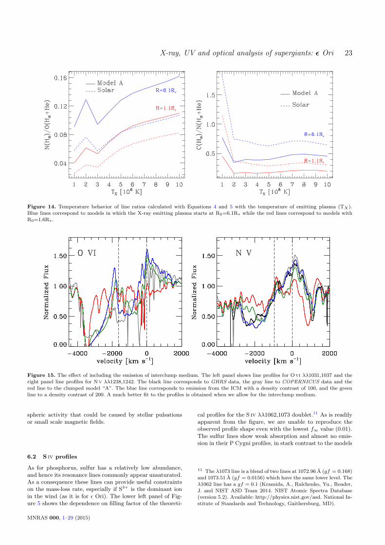
X-ray, UV and optical analysis of supergiants: ǫ Ori 23
Figure 14. Temperature behavior of line ratios calculated with Equations 4 and 5 with the temperature of emitting plasma (TX).Blue lines correspond to models in which the X-ray emitting plasma starts at R0=6.1R∗ while the red lines correspond to models withR0=1.6R∗.
Figure 15. The effect of including the emission of interclump medium. The left panel shows line profiles for Ovi λλ1031,1037 and the
right panel line profiles for Nv λλ1238,1242. The black line corresponds to GHRS data, the gray line to COPERNICUS data and thered line to the clumped model “A”. The blue line corresponds to emission from the ICM with a density contrast of 100, and the greenline to a density contrast of 200. A much better fit to the profiles is obtained when we allow for the interclump medium.
spheric activity that could be caused by stellar pulsationsor small scale magnetic fields.
6.2 S iv profiles
As for phosphorus, sulfur has a relatively low abundance,and hence its resonance lines commonly appear unsaturated.As a consequence these lines can provide useful constraintson the mass-loss rate, especially if S3+ is the dominant ionin the wind (as it is for ǫ Ori). The lower left panel of Fig-ure 5 shows the dependence on filling factor of the theoreti-
cal profiles for the S iv λλ1062,1073 doublet.11 As is readilyapparent from the figure, we are unable to reproduce theobserved profile shape even with the lowest f∞ value (0.01).The sulfur lines show weak absorption and almost no emis-sion in their P Cygni profiles, in stark contrast to the models
11 The λ1073 line is a blend of two lines at 1072.96 A (gf = 0.168)and 1073.51 A (gf = 0.0156) which have the same lower level. Theλ1062 line has a gf = 0.1 (Kramida, A., Ralchenko, Yu., Reader,J. and NIST ASD Team 2014. NIST Atomic Spectra Database(version 5.2). Available: http://physics.nist.gov/asd. National In-stitute of Standards and Technology, Gaithersburg, MD).
MNRAS 000, 1–29 (2015)

24 Raul E. Puebla et al.
Figure 16. Sobolev line optical depth for Nv λ1238 A (solid) andOvi λ1032 A (dashed). The red lines correspond to the clumpedmodel “A”, while the blue and green lines are for the interclumpmedium models with density contrasts of 100 and 200 respec-
tively.
Figure 17. Hα profiles from model “A”. Rotation is accountedfor using different methods: convolution with a 70 km s−1 kernel(blue), 2D profile with v sin i=70 km s−1 (red) and 2D profilewith v sin i=40 km s−1 (green) (see text for details).
that show strong emission and blue absorption. Particularlystriking is the absence of absorption at high velocities.
As shown in Figure 19, we can only “fit” the sulfurdoublet if we use an absurdly low abundance (∼0.2 S⊙ withf∞=0.1) or filling factor (f∞∼0.005). Even with this abun-dance, the calculated line profiles show more emission thanthe data. Moreover, an abundance of 0.2 S⊙ is incompati-ble with other UV and optical sulfur lines (e.g., S iv λ1098-1100,4486 and S iii λ4254). This problem is quite similar tothat reported previously with P v λλ1117,1128 in O stars(e.g. Hillier 2003; Bouret et al. 2003; Fullerton et al. 2006,2008; Bouret et al. 2012), and hence we consider similar so-lutions.
Various solutions have been proposed for solving thePv λ1117,1128 problem, including the following:
(i) Sub-solar abundance. While factors of 2 variation be-tween stars cannot be ruled out, much larger variations are
unlikely. In the present case, other S lines rule this out asthe main cause.
(ii) Wrong wind ionization, possibly due to the influenceof X-rays. However, the required X-ray flux is higher thanobserved.
(iii) Wrong wind ionization, possibly because the bulk ofthe wind has been shocked and not cooled.
(iv) The wind is porous spatially, or porous in velocityspace (hereafter called vorosity). Porosity will affect bothobserved X-ray and UV line profiles, whereas vorosity willonly affect UV line profiles.
The influence of X-rays on the ionization structurewas analyzed by Marcolino et al. (2009) in the context ofthe weak wind problem of late O dwarf stars. They foundthat the X-ray luminosity necessary to fit the C iv linestrength is approximately 3 dex above the standard value ofL/Lbol=− 7.0. In the same sense, Krticka & Kubat (2009,2012) explored the influence of X-rays on the phosphorousion fraction q(P+4) aiming to fit the Pv lines. They con-cluded that hard X-ray emission does not have a strong ef-fect on q(P+4), whereas XUV (54 - 124 ev) emission yields aq(P+4) according to observations. However, X-ray and XUVemission affects the ionization structure of other ions (e.g.Cvi, N iv and O iii). This influences the wind terminal ve-locity value in a non-negligible way, contradicting the obser-vations (Krticka & Kubat 2012).
In our models the influence of X-rays on the ioniza-tion fraction of S+3 is less than 5% for the clumped winds(f∞ = 0.01 − 0.1), while for the smooth wind the q(S+3)is ∼25%. Manipulating the fX values for the cold plasma(1×10⁶ K), we computed a model with an enhanced emissionin the range of 160-250 A, just above the ionization thresh-old of S iv. We found that even though the bluer absorptioncomponent of S iv lines is weakened, it wasn’t enough tofit the observed profiles. Furthermore, the XUV radiationneeded to fit the lines would be extremely high. Moreover,we obtained reasonable S iv profiles setting R0 deeper in thewind (R0=1.1 R∗). Nevertheless, this change increases thePv abundance in such a way that the lines Pv λλ1118,1128become too strong. Besides that, such R0 value is ruled outby X-ray analysis.
Macroclumping (porosity) could reproduce the reso-nance lines of Pv without requiring extremely low mass-lossrates, since optically thick clumps will reduce the effectiveopacity of the lines (e.g. Owocki 2008; Oskinova et al. 2007).
Another effect to be taken into account is the so-called“velocity-porosity” or vorosity (Owocki 2008) that evaluatethe effect of a non-monotonic velocity or a velocity field withstrong jumps or holes (in the velocity space) on line radiativetransfer.
Owocki (2008) showed that vorosity yields a reduc-tion in line absorption but it is low (10-20%). This makesthe vorosity effects weak when compared with porosityones. However, simulation from Sundqvist et al. (2010) andSundqvist et al. (2011) (see also Sundqvist et al. 2014) pointout that vorosity has an important effect on UV profiles thatimproves the agreement between optical and UV line mass-loss rates.
Using 3D Monte-Carlo simulations Surlan et al. (2012,2013) argue that porosity dominates over vorosity effects. Anissue with all of these studies is that they primarily utilize
MNRAS 000, 1–29 (2015)
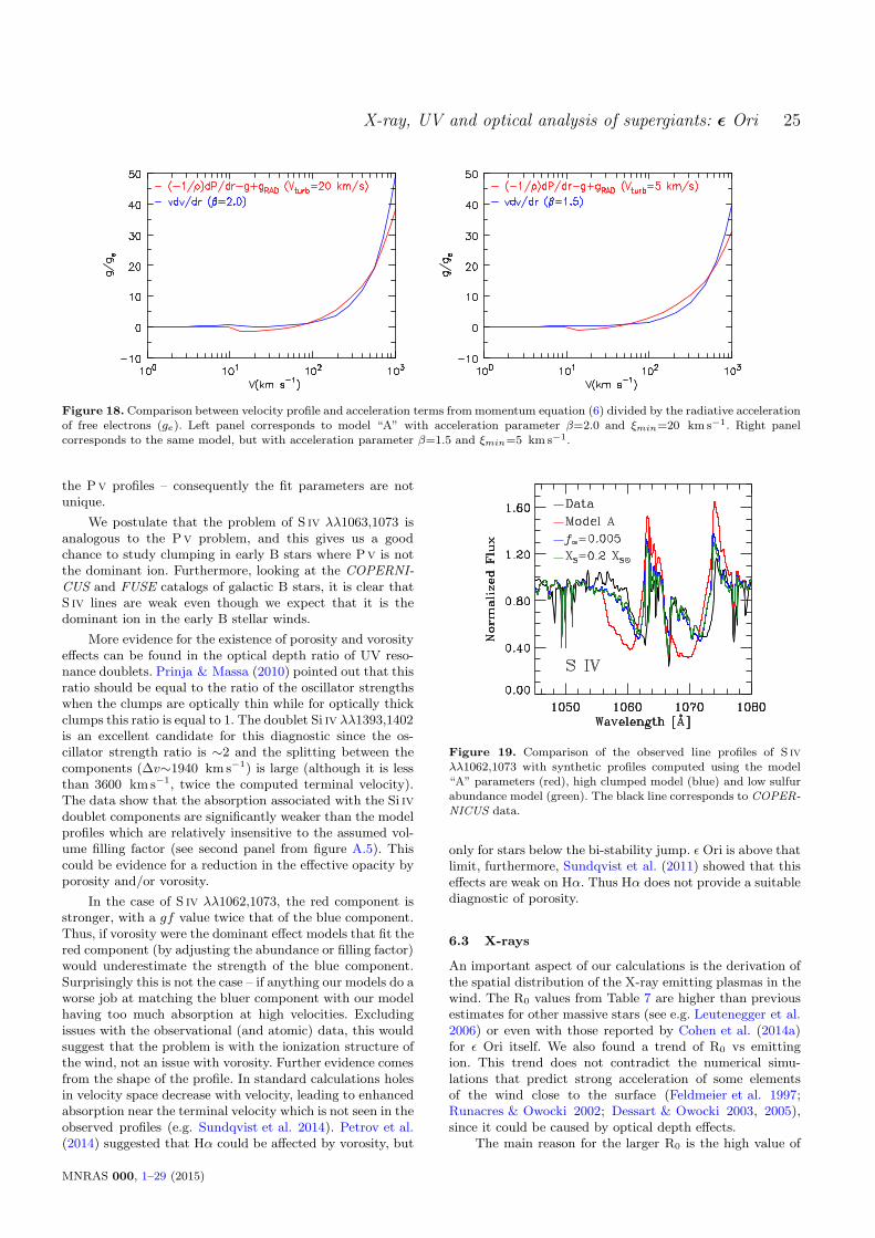
X-ray, UV and optical analysis of supergiants: ǫ Ori 25
Figure 18. Comparison between velocity profile and acceleration terms frommomentum equation (6) divided by the radiative accelerationof free electrons (ge). Left panel corresponds to model “A” with acceleration parameter β=2.0 and ξmin=20 km s−1. Right panelcorresponds to the same model, but with acceleration parameter β=1.5 and ξmin=5 km s−1.
the Pv profiles – consequently the fit parameters are notunique.
We postulate that the problem of S iv λλ1063,1073 isanalogous to the Pv problem, and this gives us a goodchance to study clumping in early B stars where Pv is notthe dominant ion. Furthermore, looking at the COPERNI-CUS and FUSE catalogs of galactic B stars, it is clear thatS iv lines are weak even though we expect that it is thedominant ion in the early B stellar winds.
More evidence for the existence of porosity and vorosityeffects can be found in the optical depth ratio of UV reso-nance doublets. Prinja & Massa (2010) pointed out that thisratio should be equal to the ratio of the oscillator strengthswhen the clumps are optically thin while for optically thickclumps this ratio is equal to 1. The doublet Si iv λλ1393,1402is an excellent candidate for this diagnostic since the os-cillator strength ratio is ∼2 and the splitting between thecomponents (∆v∼1940 kms−1) is large (although it is lessthan 3600 km s−1, twice the computed terminal velocity).The data show that the absorption associated with the Si ivdoublet components are significantly weaker than the modelprofiles which are relatively insensitive to the assumed vol-ume filling factor (see second panel from figure A.5). Thiscould be evidence for a reduction in the effective opacity byporosity and/or vorosity.
In the case of S iv λλ1062,1073, the red component isstronger, with a gf value twice that of the blue component.Thus, if vorosity were the dominant effect models that fit thered component (by adjusting the abundance or filling factor)would underestimate the strength of the blue component.Surprisingly this is not the case – if anything our models do aworse job at matching the bluer component with our modelhaving too much absorption at high velocities. Excludingissues with the observational (and atomic) data, this wouldsuggest that the problem is with the ionization structure ofthe wind, not an issue with vorosity. Further evidence comesfrom the shape of the profile. In standard calculations holesin velocity space decrease with velocity, leading to enhancedabsorption near the terminal velocity which is not seen in theobserved profiles (e.g. Sundqvist et al. 2014). Petrov et al.(2014) suggested that Hα could be affected by vorosity, but
Figure 19. Comparison of the observed line profiles of S iv
λλ1062,1073 with synthetic profiles computed using the model“A” parameters (red), high clumped model (blue) and low sulfurabundance model (green). The black line corresponds to COPER-NICUS data.
only for stars below the bi-stability jump. ǫ Ori is above thatlimit, furthermore, Sundqvist et al. (2011) showed that thiseffects are weak on Hα. Thus Hα does not provide a suitablediagnostic of porosity.
6.3 X-rays
An important aspect of our calculations is the derivation ofthe spatial distribution of the X-ray emitting plasmas in thewind. The R0 values from Table 7 are higher than previousestimates for other massive stars (see e.g. Leutenegger et al.2006) or even with those reported by Cohen et al. (2014a)for ǫ Ori itself. We also found a trend of R0 vs emittingion. This trend does not contradict the numerical simu-lations that predict strong acceleration of some elementsof the wind close to the surface (Feldmeier et al. 1997;Runacres & Owocki 2002; Dessart & Owocki 2003, 2005),since it could be caused by optical depth effects.
The main reason for the larger R0 is the high value of
MNRAS 000, 1–29 (2015)

26 Raul E. Puebla et al.
β. With a larger β the wind velocity necessary to fit theline widths occurs at larger radii. For a model with β=1,R0 is closer to the surface, and variation of R0 with thetemperature is weaker. This is consistent with the findingof constant R0 for ǫ Ori by Cohen et al. (2014a). However,we stress that the link between R0 and β that we found inthis work, provides a new challenge for understanding shockformation in the wind and the X-ray emission of massivestars. What does R0 actually mean and what is behind itsrelation with wind acceleration? In order to understand theunderlying physics of these connections, it is necessary toexpand the analysis to more systems.
From the models it is possible to estimate the regionwhere the bulk of each component of He-like lines is emit-ted. The local contribution to line flux is proportional tor2n2
p(r)ǫ(r), where ǫ(r) is the line emissivity and np is thedensity of the emitting plasma. For instance, for Ovii Heα,the intercombination component (i) has its maximum con-tribution at ∼4.6 R∗. For the forbidden component (f), thecorresponding value is ∼28.5 R∗. These values show that thedifferent components of He-like triplets are mostly producedin different regions in the wind.
One caveat with our analysis is that our assumption of asmall set of single-temperature plasmas to describe the shockemissions is not realistic. In the inner wind the cooling time(Tcool ∼ 1/ρ) for each shock is less than the dynamic time,and hence modeling of the shock structure is required toaccurately predict the X-ray emission.This will be exploredin the future.
All of our models yield asymmetric lines, with a lowerdegree of skewness for models with lower filling factor. Theobserved blue-shifts of approximately ∼210±123 kms−1 forlines with wavelength λ&10 A provide clear evidence ofwind absorption. While a clumped wind is necessary to fitthe line profiles we cannot distinguish between the “A” or“B” models with f∞=0.1 and 0.05 respectively. Both mod-els yield adequate X-ray profiles with reasonable mass-lossrates without requiring the inclusion of porosity or resonancescattering effects. This confirms the mass-loss rate derivedby Cohen et al. (2014a) that did not use porosity effectsto fit X-ray line profiles. Even though, our results and theCohen et al. ones cannot confirm the absence of porosity.Much higher signal-to-noise X-ray observations are neededif tighter constraints are to be obtained. Moreover, due tothe strong variability of Hα, the influence of non-sphericalwinds and temporal variability should be considered.
It is generally assumed that X-rays don’t strongly affectthe X-ray opacity of the “cool” wind. In the case of ǫ Oriwe found that this is not necessarily true. In ǫ Ori the X-rays can ionize He+ in the outer wind (Fig. 20), reducingthe X-ray opacity (see the behaviour at outer regions of thered line in Fig. 10). The effect is largest in the unclumpedmodel. Normally, X-rays don’t strongly affect the dominantionization stage as X-ray flux is generally small comparedwith the UV ionizing flux near the relevant thresholds – thisis not the case for ǫ Ori.
The effect of X-rays on He ionization in wind has twoconsequences: 1) For modeling B or later stars, it is impor-tant to take into account the interaction of X-rays with thewind consistently in order to estimate the wind parameters,and not separately as commonly done for O stars. 2) Thevalue of the mass-loss rates computed using X-ray line pro-
files may be biased toward low values if this effect is nottaken into account.
Finally, our preferred models, A and B, show a verystrong trend of higher X-ray filling factors for low temper-ature emission components (see table 7). This model fit-ting result accounts for both wind absorption and the dif-ferent emissivities of different plasma temperature compo-nents, and thus reflects the instantaneous plasma tempera-ture distribution. These results are broadly consistent with ashock-heating analysis that shows a very strong preferencefor weaker shocks over strong ones, with almost no shockheating above 107 K.
7 SUMMARY AND CONCLUSIONS
We have presented a multi-wavelength analysis of the earlyB supergiant ǫ Ori. This analysis utilizes a modified versionof cmfgen that allows for the radiative interactions betweenthe X-ray emitting plasma and the cool wind.
We get excellent fits to X-ray, UV and optical data.The derived photospheric parameters for ǫ Ori are quitesimilar to those previously derived (Teff=27000±500 Kand log g=3.0±0.05). The observed UV fluxes together withthe known mV yields E(B-V)=0.091±0.01. Using the lastHIPPARCOS distance (606 pc), the ǫ Ori luminosity islog(L∗/L⊙)∼5.93. This luminosity is the highest reportedvalue for ǫ Ori. Using the former HIPPARCOS distance (412pc), the ǫ Ori luminosity is log(L∗/L⊙)∼5.60.
The metal abundances derived from the different pass-bands (X-ray, optical and UV) are consistent within errors.We derive [N/O]=0.15 and [N/C]=0.33 for ǫ Ori. Opticallyderived CNO abundances show a factor of two dispersionabout the mean, suggesting there are still some inadequaciesin the atomic models, and/or the treatment of turbulence.
The UV S iv λλ1068,1073 profiles show the same prob-lem as reported for Pv λλ1117,1128 in O stars (e.g.,Fullerton et al. 2006). To fit this doublet (actually threelines but two are blended) it is necessary to use an extremelyclumped wind and/or a very low sulfur abundance. The lat-ter is incompatible with other UV and optical sulfur lines.Close examination of the profiles suggests an issue with thecalculated ionization structure of the outer wind (possiblyrelated to the presence of a hot plasma), although porosityand vorosity effects may also be important.
A clumped wind, with a volume filling factor of order0.1 or less, produces X-ray profiles consistent with obser-vation, favoring M64.9×10−7 M⊙ yr−1, a value approxi-mately 4 times lower than the one theoretically predicted byVink et al. (2000, 2001). However the signal-to-noise ratio ofthe X-ray data does not allow us to determine an accuratefX value, or to examine the effects of porosity. We also foundevidence that the UV profiles Si iv and S iv could be affectedby porosity or problems with the ionization structure.
As found for ζ Pup (Zsargo et al. 2008), we found evi-dence of resonance scattering from the interclump medium– the traditional clumped model cannot reproduce the ob-served Ovi and Nv resonance profiles.
The β=2 value reported in this work is higher thanfound in earlier work, and than that expected from stan-dard wind theory. However the observed Hα is variable, and
MNRAS 000, 1–29 (2015)
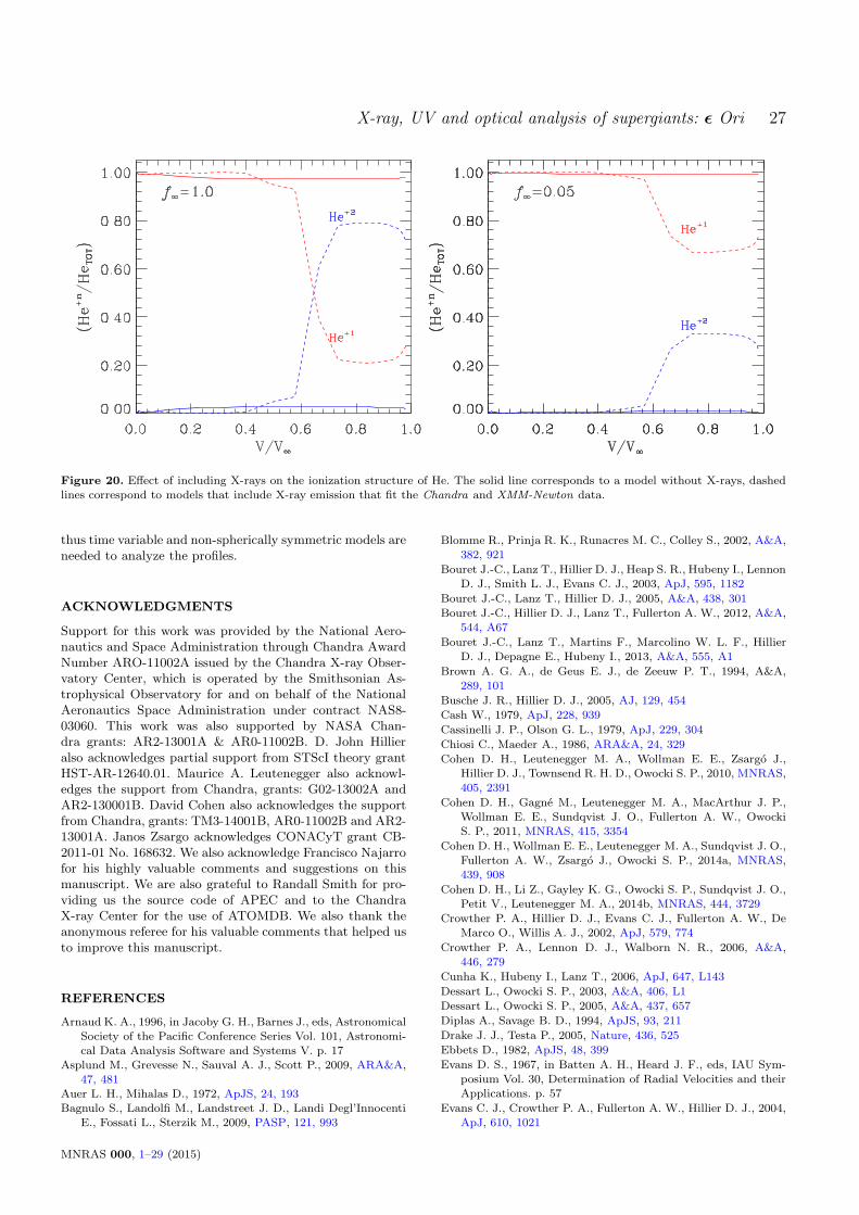
X-ray, UV and optical analysis of supergiants: ǫ Ori 27
Figure 20. Effect of including X-rays on the ionization structure of He. The solid line corresponds to a model without X-rays, dashedlines correspond to models that include X-ray emission that fit the Chandra and XMM-Newton data.
thus time variable and non-spherically symmetric models areneeded to analyze the profiles.
ACKNOWLEDGMENTS
Support for this work was provided by the National Aero-nautics and Space Administration through Chandra AwardNumber ARO-11002A issued by the Chandra X-ray Obser-vatory Center, which is operated by the Smithsonian As-trophysical Observatory for and on behalf of the NationalAeronautics Space Administration under contract NAS8-03060. This work was also supported by NASA Chan-dra grants: AR2-13001A & AR0-11002B. D. John Hillieralso acknowledges partial support from STScI theory grantHST-AR-12640.01. Maurice A. Leutenegger also acknowl-edges the support from Chandra, grants: G02-13002A andAR2-130001B. David Cohen also acknowledges the supportfrom Chandra, grants: TM3-14001B, AR0-11002B and AR2-13001A. Janos Zsargo acknowledges CONACyT grant CB-2011-01 No. 168632. We also acknowledge Francisco Najarrofor his highly valuable comments and suggestions on thismanuscript. We are also grateful to Randall Smith for pro-viding us the source code of APEC and to the ChandraX-ray Center for the use of ATOMDB. We also thank theanonymous referee for his valuable comments that helped usto improve this manuscript.
REFERENCES
Arnaud K. A., 1996, in Jacoby G. H., Barnes J., eds, AstronomicalSociety of the Pacific Conference Series Vol. 101, Astronomi-cal Data Analysis Software and Systems V. p. 17
Asplund M., Grevesse N., Sauval A. J., Scott P., 2009, ARA&A,47, 481
Auer L. H., Mihalas D., 1972, ApJS, 24, 193Bagnulo S., Landolfi M., Landstreet J. D., Landi Degl’Innocenti
E., Fossati L., Sterzik M., 2009, PASP, 121, 993
Blomme R., Prinja R. K., Runacres M. C., Colley S., 2002, A&A,382, 921
Bouret J.-C., Lanz T., Hillier D. J., Heap S. R., Hubeny I., LennonD. J., Smith L. J., Evans C. J., 2003, ApJ, 595, 1182
Bouret J.-C., Lanz T., Hillier D. J., 2005, A&A, 438, 301
Bouret J.-C., Hillier D. J., Lanz T., Fullerton A. W., 2012, A&A,544, A67
Bouret J.-C., Lanz T., Martins F., Marcolino W. L. F., HillierD. J., Depagne E., Hubeny I., 2013, A&A, 555, A1
Brown A. G. A., de Geus E. J., de Zeeuw P. T., 1994, A&A,289, 101
Busche J. R., Hillier D. J., 2005, AJ, 129, 454
Cash W., 1979, ApJ, 228, 939
Cassinelli J. P., Olson G. L., 1979, ApJ, 229, 304
Chiosi C., Maeder A., 1986, ARA&A, 24, 329
Cohen D. H., Leutenegger M. A., Wollman E. E., Zsargo J.,Hillier D. J., Townsend R. H. D., Owocki S. P., 2010, MNRAS,405, 2391
Cohen D. H., Gagne M., Leutenegger M. A., MacArthur J. P.,Wollman E. E., Sundqvist J. O., Fullerton A. W., OwockiS. P., 2011, MNRAS, 415, 3354
Cohen D. H., Wollman E. E., Leutenegger M. A., Sundqvist J. O.,Fullerton A. W., Zsargo J., Owocki S. P., 2014a, MNRAS,439, 908
Cohen D. H., Li Z., Gayley K. G., Owocki S. P., Sundqvist J. O.,Petit V., Leutenegger M. A., 2014b, MNRAS, 444, 3729
Crowther P. A., Hillier D. J., Evans C. J., Fullerton A. W., DeMarco O., Willis A. J., 2002, ApJ, 579, 774
Crowther P. A., Lennon D. J., Walborn N. R., 2006, A&A,446, 279
Cunha K., Hubeny I., Lanz T., 2006, ApJ, 647, L143
Dessart L., Owocki S. P., 2003, A&A, 406, L1
Dessart L., Owocki S. P., 2005, A&A, 437, 657
Diplas A., Savage B. D., 1994, ApJS, 93, 211
Drake J. J., Testa P., 2005, Nature, 436, 525
Ebbets D., 1982, ApJS, 48, 399
Evans D. S., 1967, in Batten A. H., Heard J. F., eds, IAU Sym-posium Vol. 30, Determination of Radial Velocities and theirApplications. p. 57
Evans C. J., Crowther P. A., Fullerton A. W., Hillier D. J., 2004,ApJ, 610, 1021
MNRAS 000, 1–29 (2015)
28 Raul E. Puebla et al.
Eversberg T., Lepine S., Moffat A. F. J., 1998, ApJ, 494, 799
Feldmeier A., Puls J., Pauldrach A. W. A., 1997, A&A, 322, 878
Foster A. R., Ji L., Smith R. K., Brickhouse N. S., 2012, ApJ,756, 128
Fullerton A. W., Gies D. R., Bolton C. T., 1996, ApJS, 103, 475
Fullerton A. W., Massa D. L., Prinja R. K., 2006, ApJ, 637, 1025Fullerton A. W., Massa D. L., Prinja R. K., 2008, in Hamann W.-
R., Feldmeier A., Oskinova L. M., eds, Clumping in Hot-StarWinds. p. 23
Gabriel A. H., Jordan C., 1969, MNRAS, 145, 241
Gray D. F., 2008, The Observation and Analysis of Stellar Pho-tospheres. Cambridge University Press, 2008
Harnden Jr. F. R., et al., 1979, ApJ, 234, L51
Hearn A. G., 1975, A&A, 40, 355Herve A., Rauw G., Naze Y., 2013, A&A, 551, A83
Hillier D. J., 1991, A&A, 247, 455Hillier D. J., 2003, in I. Hubeny, D. Mihalas, & K. Werner ed., As-
tronomical Society of the Pacific Conference Series Vol. 288,
Stellar Atmosphere Modeling. pp 199–+Hillier D. J., Miller D. L., 1998, ApJ, 496, 407
Hillier D. J., Miller D. L., 1999, ApJ, 519, 354Hillier D. J., Bouret J.-C., Lanz T., Busche J. R., 2012, MNRAS,
426, 1043
Howarth I., Lamers H. J. G., 1999, Journal of the British Astro-nomical Association, 109, 347
Howarth I. D., Siebert K. W., Hussain G. A. J., Prinja R. K.,1997, MNRAS, 284, 265
Ignace R., Gayley K. G., 2002, ApJ, 568, 954
Kaper L., Henrichs H. F., Nichols J. S., Snoek L. C., Volten H.,Zwarthoed G. A. A., 1996, A&AS, 116, 257
Knobel E. B., 1909, The Observatory, 32, 357
Krticka J., Kubat J., 2009, MNRAS, 394, 2065Krticka J., Kubat J., 2012, MNRAS, 427, 84
Kudritzki R. P., Puls J., Lennon D. J., Venn K. A., Reetz J.,Najarro F., McCarthy J. K., Herrero A., 1999, A&A, 350, 970
Lamers H. J. G. L. M., 1974, A&A, 37, 237Lamers H. J. G. L. M., Leitherer C., 1993, ApJ, 412, 771
Lee T. A., 1968, ApJ, 152, 913Lesh J. R., 1968, ApJS, 17, 371
Leutenegger M. A., Paerels F. B. S., Kahn S. M., Cohen D. H.,2006, ApJ, 650, 1096
Leutenegger M. A., Owocki S. P., Kahn S. M., Paerels F. B. S.,2007, ApJ, 659, 642
Leutenegger M. A., Cohen D. H., Zsargo J., Martell E. M.,MacArthur J. P., Owocki S. P., Gagne M., Hillier D. J., 2010,ApJ, 719, 1767
Leutenegger M. A., Cohen D. H., Sundqvist J. O., Owocki S. P.,2013, ApJ, 770, 80
Lucy L. B., 1982, ApJ, 255, 286
Lucy L. B., 2010, A&A, 524, A41Lucy L. B., White R. L., 1980, ApJ, 241, 300
Macfarlane J. J., Cassinelli J. P., Welsh B. Y., Vedder P. W.,Vallerga J. V., Waldron W. L., 1991, ApJ, 380, 564
Macfarlane J. J., Cohen D. H., Wang P., 1994, ApJ, 437, 351Maeder A., Meynet G., 2000, ARA&A, 38, 143
Marcolino W. L. F., Bouret J.-C., Martins F., Hillier D. J., LanzT., Escolano C., 2009, A&A, 498, 837
Martins F., Hillier D. J., 2012, A&A, 545, A95
Martins F., Schaerer D., Hillier D. J., Meynadier F., Heydari-Malayeri M., Walborn N. R., 2005, A&A, 441, 735
Martins F., Marcolino W., Hillier D. J., Donati J.-F., Bouret J.-
C., 2015, A&A, 574, A142McErlean N. D., Lennon D. J., Dufton P. L., 1998, A&A, 329, 613
McErlean N. D., Lennon D. J., Dufton P. L., 1999, A&A, 349, 553Morel T., Marchenko S. V., Pati A. K., Kuppuswamy K., Carini
M. T., Wood E., Zimmerman R., 2004, MNRAS, 351, 552
Najarro F., Hillier D. J., Puls J., Lanz T., Martins F., 2006, A&A,456, 659
Najarro F., Hanson M. M., Puls J., 2011, A&A, 535, A32
Nieva M. F., Przybilla N., 2006, ApJ, 639, L39
Oskinova L. M., Feldmeier A., Hamann W.-R., 2006, MNRAS,372, 313
Oskinova L. M., Hamann W.-R., Feldmeier A., 2007, A&A,476, 1331
Oskinova L., Hamann W.-R., Ignace R., Feldmeier A., 2011, Bul-letin de la Societe Royale des Sciences de Liege, 80, 54
Owocki S. P., 2008, in Hamann W.-R., Feldmeier A., Oskinova
L. M., eds, Clumping in Hot-Star Winds. p. 121Owocki S. P., Cohen D. H., 2001, ApJ, 559, 1108
Owocki S. P., Cohen D. H., 2006, ApJ, 648, 565Owocki S. P., Castor J. I., Rybicki G. B., 1988, ApJ, 335, 914
Perryman M. A. C., et al., 1997, A&A, 323, L49Petit P., Louge T., Theado S., Paletou F., Manset N., Morin J.,
Marsden S. C., Jeffers S. V., 2014, PASP, 126, 469
Petrov B., Vink J. S., Grafener G., 2014, A&A, 565, A62
Porquet D., Mewe R., Dubau J., Raassen A. J. J., Kaastra J. S.,2001, A&A, 376, 1113
Prinja R. K., Massa D. L., 2010, A&A, 521, L55
Prinja R. K., Massa D., Fullerton A. W., 2002, A&A, 388, 587Prinja R. K., Rivinius T., Stahl O., Kaufer A., Foing B. H., Cami
J., Orlando S., 2004, A&A, 418, 727
Prinja R. K., Markova N., Scuderi S., Markov H., 2006, A&A,457, 987
Puls J., Urbaneja M. A., Venero R., Repolust T., Springmann U.,Jokuthy A., Mokiem M. R., 2005, A&A, 435, 669
Puls J., Markova N., Scuderi S., Stanghellini C., Taranova O. G.,Burnley A. W., Howarth I. D., 2006, A&A, 454, 625
Repolust T., Puls J., Hanson M. M., Kudritzki R.-P., MokiemM. R., 2005, A&A, 440, 261
Rivero Gonzalez J. G., Puls J., Najarro F., 2011, A&A, 536, A58
Rivero Gonzalez J. G., Puls J., Najarro F., Brott I., 2012a, A&A,537, A79
Rivero Gonzalez J. G., Puls J., Massey P., Najarro F., 2012b,A&A, 543, A95
Runacres M. C., Owocki S. P., 2002, A&A, 381, 1015
Santolaya-Rey A. E., Puls J., Herrero A., 1997, A&A, 323, 488Savage B. D., Bohlin R. C., Drake J. F., Budich W., 1977, ApJ,
216, 291
Searle S. C., Prinja R. K., Massa D., Ryans R., 2008, A&A,481, 777
Seward F. D., Forman W. R., Giacconi R., Griffiths R. E., Harn-den Jr. F. R., Jones C., Pye J. P., 1979, ApJ, 234, L55
Silvester J., Wade G. A., Kochukhov O., Bagnulo S., Folsom C. P.,Hanes D., 2012, MNRAS, 426, 1003
Simon-Dıaz S., Herrero A., 2007, A&A, 468, 1063Smith R. K., Brickhouse N. S., Liedahl D. A., Raymond J. C.,
2001, ApJ, 556, L91Snow Jr. T. P., Morton D. C., 1976, ApJS, 32, 429
Sundqvist J. O., Puls J., Feldmeier A., 2010, A&A, 510, A11Sundqvist J. O., Puls J., Feldmeier A., Owocki S. P., 2011, A&A,
528, A64
Sundqvist J. O., Owocki S. P., Cohen D. H., Leutenegger M. A.,Townsend R. H. D., 2012, MNRAS, 420, 1553
Sundqvist J. O., Puls J., Owocki S. P., 2014, A&A, 568, A59Thompson G. B., Morrison N. D., 2013, AJ, 145, 95
Trundle C., Lennon D. J., 2005, A&A, 434, 677Trundle C., Lennon D. J., Puls J., Dufton P. L., 2004, A&A,
417, 217
Urbaneja M., 2004, PhD thesis, University of La LagunaVerner D. A., Yakovlev D. G., 1995, A&AS, 109, 125
Vink J. S., de Koter A., Lamers H. J. G. L. M., 2000, A&A,362, 295
Vink J. S., de Koter A., Lamers H. J. G. L. M., 2001, A&A,369, 574
Walborn N. R., 1976, ApJ, 205, 419
Waldron W. L., Cassinelli J. P., 2007, ApJ, 668, 456
MNRAS 000, 1–29 (2015)

X-ray, UV and optical analysis of supergiants: ǫ Ori 29
Zsargo J., Hillier D. J., Bouret J.-C., Lanz T., Leutenegger M. A.,
Cohen D. H., 2008, ApJ, 685, L149Surlan B., Hamann W.-R., Kubat J., Oskinova L. M., Feldmeier
A., 2012, A&A, 541, A37Surlan B., Hamann W.-R., Aret A., Kubat J., Oskinova L. M.,
Torres A. F., 2013, A&A, 559, A130van Leeuwen F., 2007, A&A, 474, 653
APPENDIX A
In this appendix we present best fit model for each filling fac-tor used in this work f∞=1.0 (red), 0.1 (blue), 0.05 (green)and 0.01 (orange). Figures A.1 to A.3 show the data (black)and the models in the optical band. Figure A.4 shows theCOPERNICUS data (black) and the models in FUV. Fig-ure A.5 shows the IUE data (black) and the models in UV.The shown models have a rotation v sin i=70 kms−1andvmacro=70 km s−1.
This paper has been typeset from a TEX/LATEX file prepared bythe author.
MNRAS 000, 1–29 (2015)

30 Raul E. Puebla et al.
Figure A.1. Best model fits for ǫ Ori for each f∞ value: 1.0 (red), 0.1 (blue), 0.05 (green) and 0.01 (orange). Optical data are shownby the black line.
MNRAS 000, 1–29 (2015)
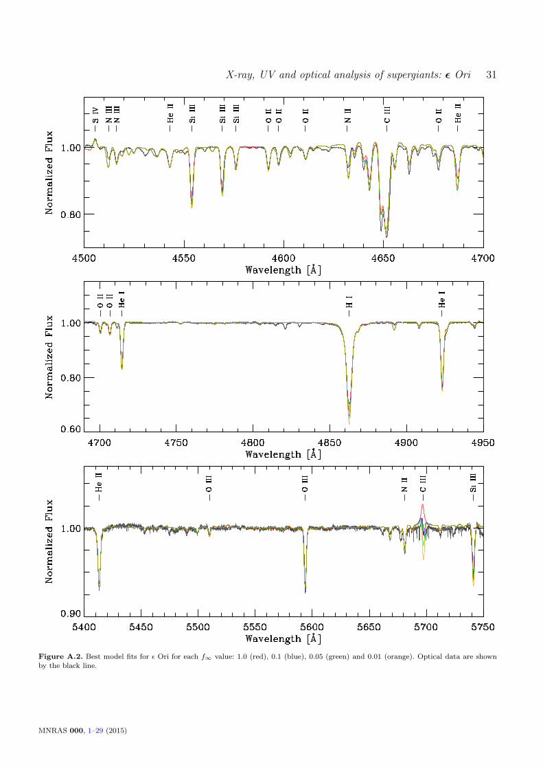
X-ray, UV and optical analysis of supergiants: ǫ Ori 31
Figure A.2. Best model fits for ǫ Ori for each f∞ value: 1.0 (red), 0.1 (blue), 0.05 (green) and 0.01 (orange). Optical data are shownby the black line.
MNRAS 000, 1–29 (2015)
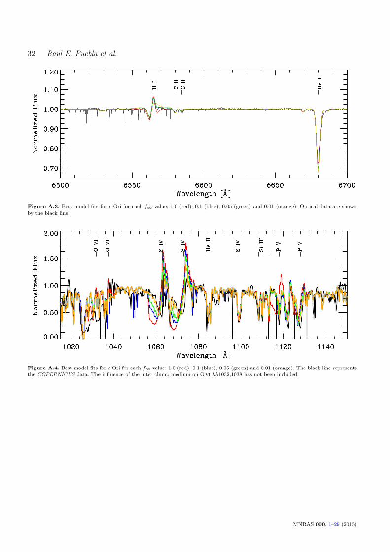
32 Raul E. Puebla et al.
Figure A.3. Best model fits for ǫ Ori for each f∞ value: 1.0 (red), 0.1 (blue), 0.05 (green) and 0.01 (orange). Optical data are shownby the black line.
Figure A.4. Best model fits for ǫ Ori for each f∞ value: 1.0 (red), 0.1 (blue), 0.05 (green) and 0.01 (orange). The black line representsthe COPERNICUS data. The influence of the inter clump medium on Ovi λλ1032,1038 has not been included.
MNRAS 000, 1–29 (2015)

X-ray, UV and optical analysis of supergiants: ǫ Ori 33
Figure A.5. Best model fits for ǫ Ori for each f∞ value: 1.0 (red), 0.1 (blue), 0.05 (green) and 0.01 (orange). The black line representsthe IUE data. The influence of the inter clump medium on Nv λλ1238,1242 has not been included.
MNRAS 000, 1–29 (2015)