X-ray Absorption Spectroscopy · X-ray Absorption Fine Structure Spectroscopy GRANT BUNKER...
86
X-ray Absorption Spectroscopy Overview of XAFS Spectroscopy and its uses Theory (a little) Experiment (a little) Data Analysis (a little) Conclusion Grant Bunker Professor and Chair Department of Physics Illinois Institute of Technology
Transcript of X-ray Absorption Spectroscopy · X-ray Absorption Fine Structure Spectroscopy GRANT BUNKER...
X-ray Absorption Spectroscopy
Overview of XAFS Spectroscopy and its uses
Theory (a little)
Experiment (a little)
Data Analysis (a little)
Conclusion
Grant Bunker Professor and Chair
Department of PhysicsIllinois Institute of Technology
Acknowledgements~42 years and counting
Ed Stern, Dale Sayers, Farrel Lytle, John Rehr, Bruce Bunker, Steve Heald, Tim Elam, Gerd Rosenbaum, many others...
XAFS community that grew from it
Students and postdocs

Introduction to
XAFSA Practical Guide to X-ray Absorption Fine Structure Spectroscopy
G R A N T BU N K ER
Introduction to
XAFS Introduction to XAFS
X-ray absorption fine structure spectroscopy (XAFS) is a powerful and versatile
technique for studying structures of materials in chemistry, physics, biology, and
other fields. This textbook is a comprehensive, practical guide to carrying out and
interpreting XAFS experiments.
Assuming only undergraduate-level physics and mathematics, the textbook is
ideally suited for graduate students in physics and chemistry starting XAFS-based
research. It contains concise executable example programs in Mathematica 7.
The textbook addresses experiment, theory, and data analysis, but is not tied to
specific data analysis programs or philosophies. This makes it accessible to a broad
audience in the sciences, and a useful guide for researchers entering the subject.
Supplementary material available at www.cambridge.org/9780521767750
�� Mathematica code from the book
�� Related Mathematica programs
�� Worked data analysis examples
GRANT BUNKER is Professor of Physics at the Illinois Institute of Technology. He has over 30 years’ experience in all aspects of XAFS spectroscopy, from technique development, instrumentation, and computation, to applications in biology, chemistry, and physics.
BU
NK
ER
Cover illustration: © Alan Crosthwaite.
Cover designed by Hart McLeod Ltd
concise guide to essentials of XAFS
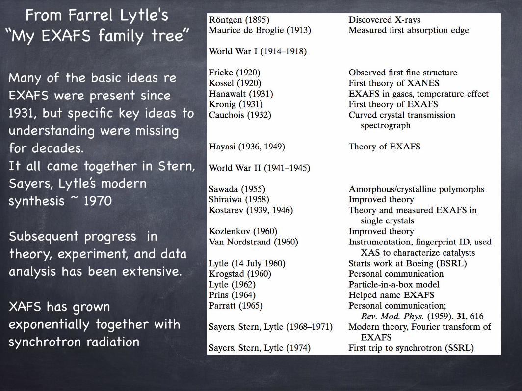
From Farrel Lytle's“My EXAFS family tree”
Many of the basic ideas re EXAFS were present since 1931, but specific key ideas to understanding were missing for decades. It all came together in Stern, Sayers, Lytle’s modern synthesis ~ 1970
Subsequent progress in theory, experiment, and data analysis has been extensive.
XAFS has grown exponentially together with synchrotron radiation
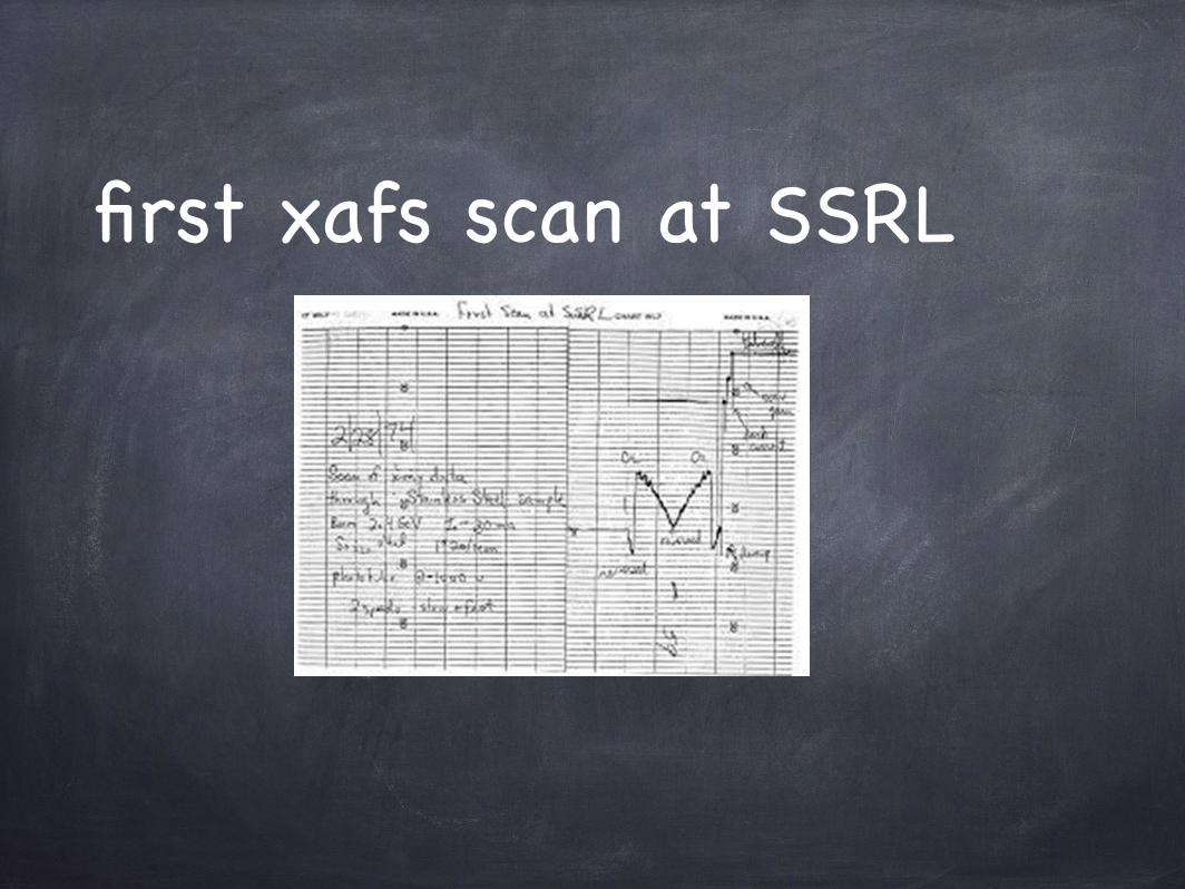
first xafs scan at SSRL

Sadly, Ed recently passed away at age 85 on May 17, 2016. Ed was an
inspired physicist who always strived to get to the essence of things. He
would invent or create whatever was necessary to do research. He also was a kind, thoughtful, person with a good
sense of humor. He will be missed.
Ed Stern, Dale Sayers, and Farrel Lytle receiving Warren Prize 1979
Some SternLab denizens
~ 1983gb in middle
Dale Sayers, a gifted and energetic physicist and teacher, tragically passed away
unexpectedly at age 60 on Nov 25, 2004
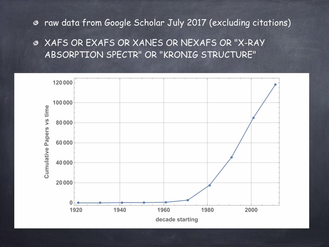
raw data from Google Scholar July 2017 (excluding citations)
XAFS OR EXAFS OR XANES OR NEXAFS OR "X-RAY ABSORPTION SPECTR" OR "KRONIG STRUCTURE"
● ● ● ● ● ●
●
●
●
●
1920 1940 1960 1980 20000
20000
40000
60000
80000
100000
120000
decade starting
CumulativePapersvstime
What is XAFS?X-ray Absorption Fine Structure spectroscopy uses the x-ray photoelectric effect and the wave nature of the electron to determine local structures around selected atomic species in materials
Unlike x-ray diffraction, it does not require long range translational order in the sample – it works equally well in amorphous materials, liquids, (poly)crystalline solids, and molecular gases.
XANES (near-edge structure) can be sensitive to charge transfer, orbital occupancy, and symmetry.
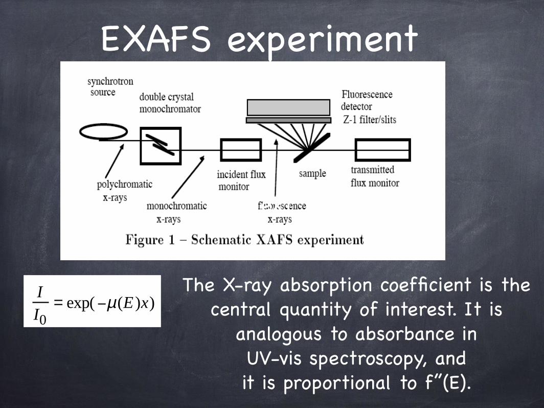
The X-ray absorption coefficient is the central quantity of interest. It is
analogous to absorbance inUV-vis spectroscopy, and it is proportional to f’’(E).
II0
= exp(−µ(E )x)
EXAFS experiment
Text
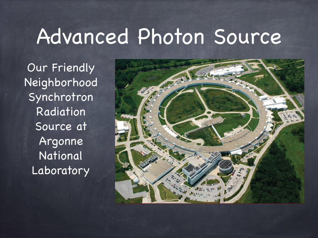
Advanced Photon Source
Our FriendlyNeighborhoodSynchrotronRadiationSource at Argonne National
Laboratory

absorption cross section, linear scale
solid: photoelectric
dotted: scattering
dashed: photoelectric + scattering
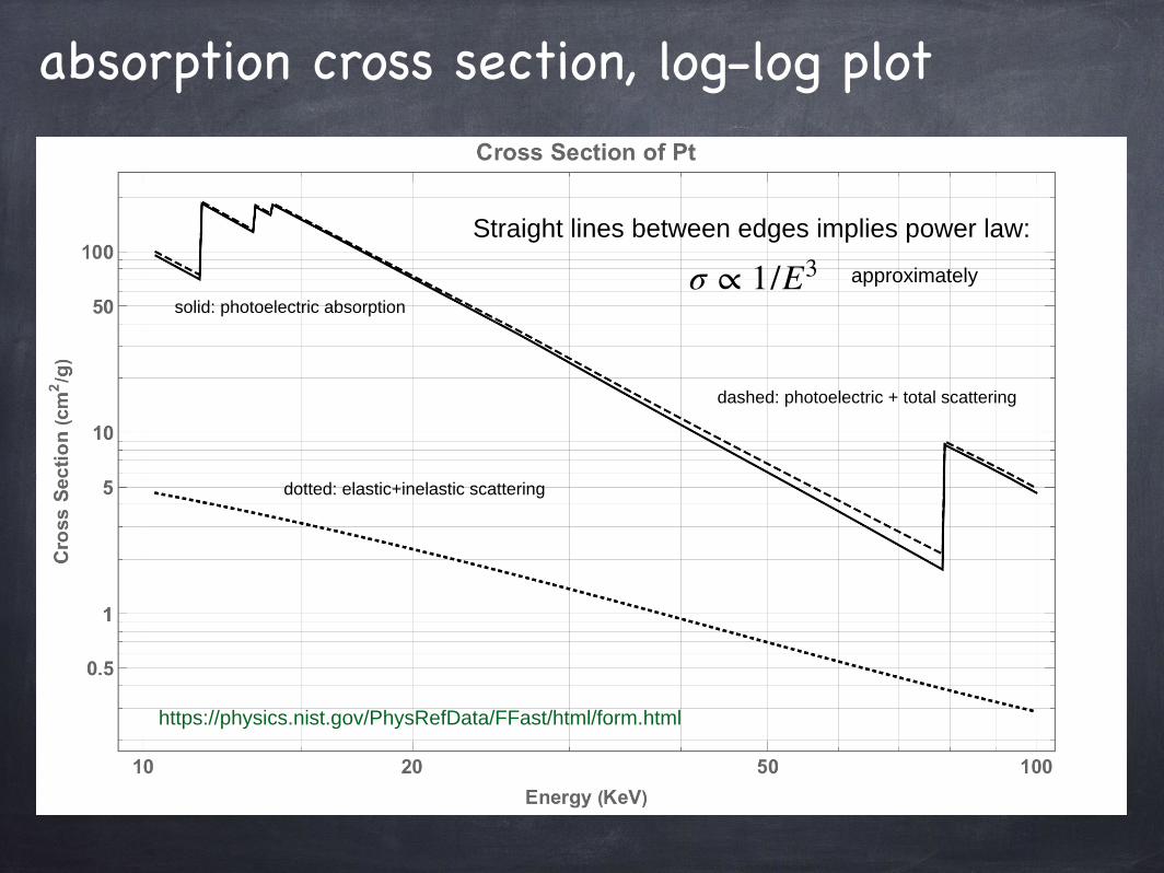
absorption cross section, log-log plot
Straight lines between edges implies power law:
dotted: elastic+inelastic scattering
dashed: photoelectric + total scattering
solid: photoelectric absorption
https://physics.nist.gov/PhysRefData/FFast/html/form.html
σ ∝ 1/E3 approximately

expt: Molecular gasesGeH4, GeH3Cl, GeCl4
tetrahedral coordination
11 000 11 100 11 200 11 300 11 400 11 500 11 600 11 7000.0
0.2
0.4
0.6
0.8
1.0
Energy HeVL
mx
GECL4.001
11 000 11 100 11 200 11 300 11 400 11 500 11 600 11 7000.0
0.2
0.4
0.6
0.8
1.0
1.2
1.4
Energy HeVL
mx
GEH3CL.001
11 000 11 100 11 200 11 300 11 400 11 500 11 600 11 7000.0
0.5
1.0
1.5
2.0
2.5
3.0
3.5
Energy HeVL
mx
GEH4.020
C. E. Bouldin, G. Bunker, D. A. McKeown, R. A. Forman, and J. J. Ritter, (1988) Phys. Rev. B 38, 10816

-0.05
0
0.05
0.1
0.15
0.2
0.25
-100 -50 0 50 100 150 200 250 300
ZnS transmission µ
x
E-E0 (eV)
XANES EXAFS
XANES+EXAFS=XAFS
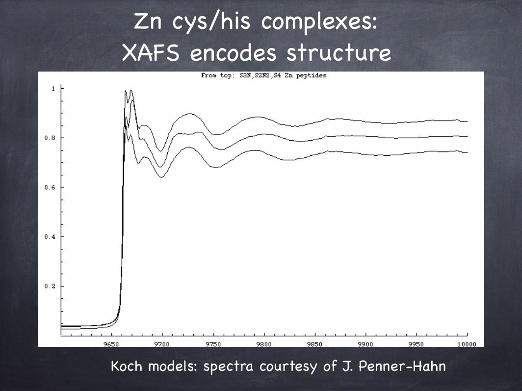
Zn cys/his complexes: XAFS encodes structure
Koch models: spectra courtesy of J. Penner-Hahn

6500 6600 6700 6800 6900 7000 71000.0
0.2
0.4
0.6
0.8
1.0
Energy HeVL
mx
MNO.080
MnOrock saltstructureT=80K

XAFS is element selectiveBy choosing the
energy of excitationyou can “tune into”different elements ina complex sample.
K-edge:Ca: 4.0 keVFe: 7.1 keVZn: 9.7 keV
Mo: 20.0 keV
EKedge ⇡ Z2.16
20/4⇡ (42/20)2.16
5020 30
10 000
5000
20 000
3000
30 000
15 000
7000
Atomic Number
Ener
gyExample:Ca vs Mo
It is usually feasible to workin a convenient energy range by choosing an appropriate edge
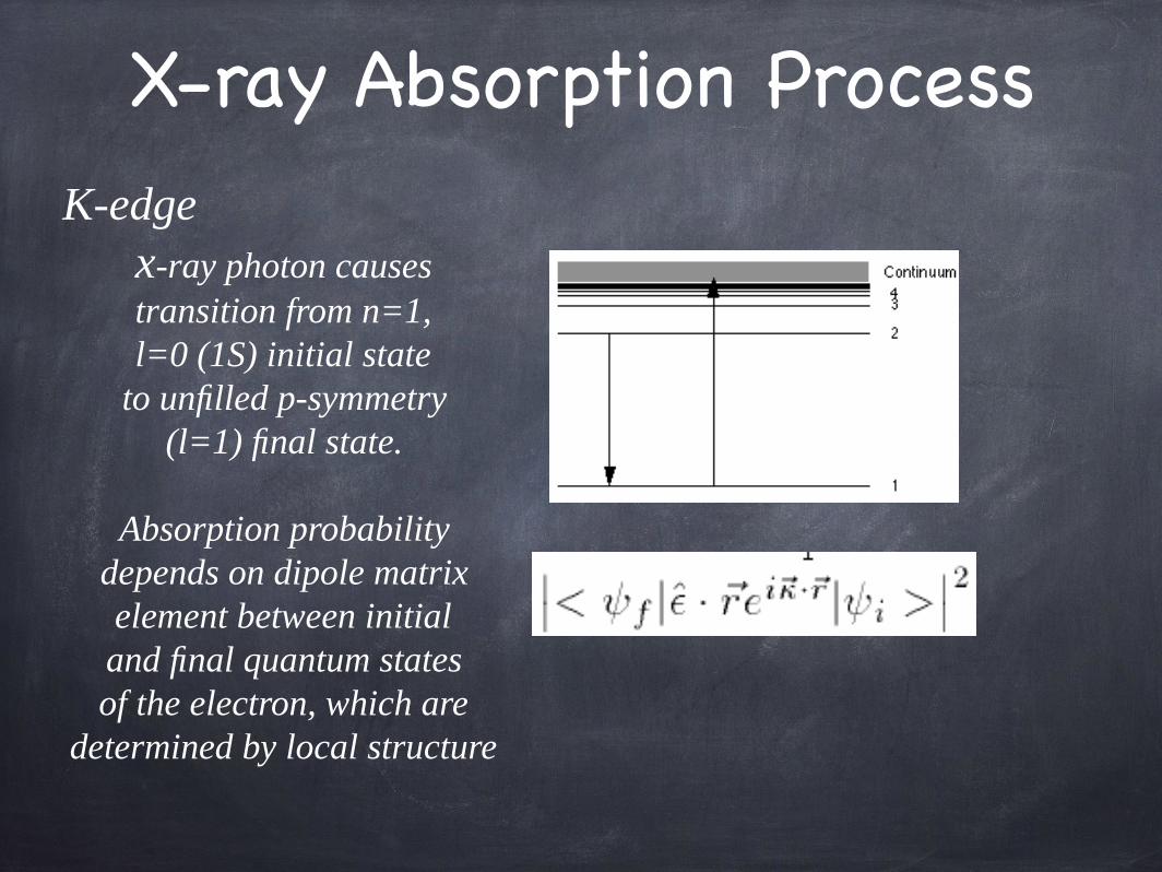
x-ray photon causestransition from n=1, l=0 (1S) initial state
to unfilled p-symmetry(l=1) final state.
Absorption probabilitydepends on dipole matrixelement between initialand final quantum statesof the electron, which are
determined by local structure
X-ray Absorption ProcessK-edge
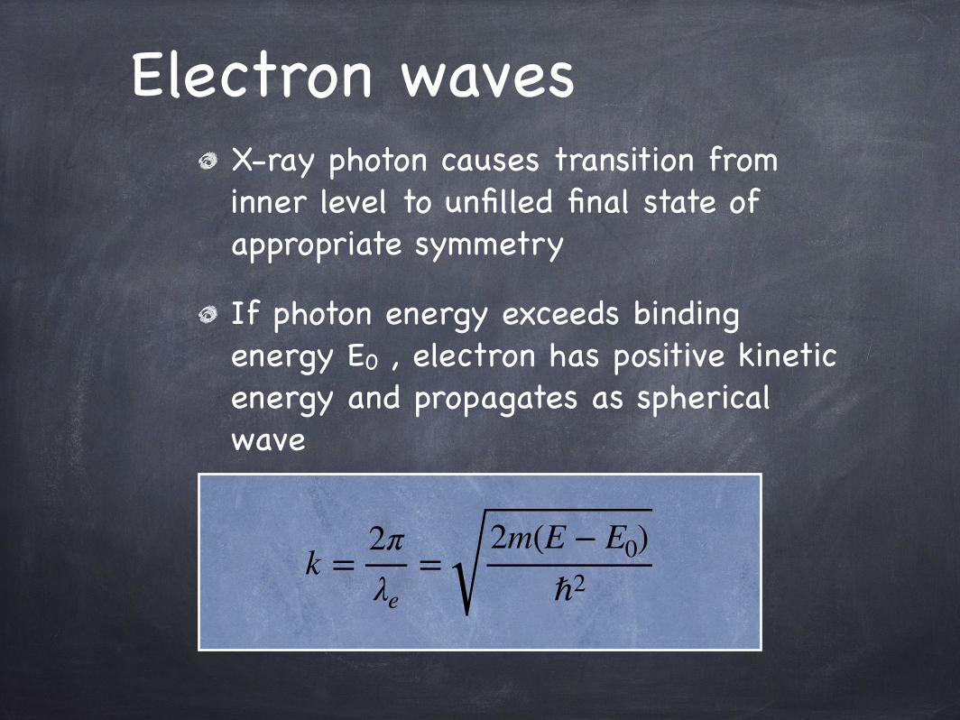
X-ray photon causes transition from inner level to unfilled final state of appropriate symmetry
If photon energy exceeds binding energy E0 , electron has positive kinetic energy and propagates as spherical wave
Electron waves
k =2πλe
=2m(E − E0)
ℏ2

Electron wave emitted by central atom is scattered by
neighboring atoms. The outgoing and scattered parts
of the final state wavefunction interfere where the initial state is localized.
Interference is constructive or destructive depending on the
distances and electron wavelength. Scanning the wavelength records an interferogram of distance distribution

Outgoing p-symmetry electron wave
Isolated atom has no final state wavefunction
interferences.
Absorption coefficient varies smoothly with electron wavelength.
This directionalitycan be useful forpolarized XAFS.

Outgoing electron wave, with scatterers (animation)
Scattering fromneighboring atoms
modifies wavefunctionnear center of absorber, modulating the energy
dependence of the transition matrix element
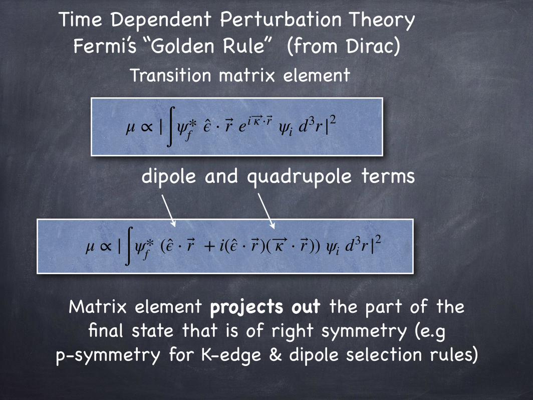
μ ∝ |∫ ψ*f ( ̂ϵ ⋅ ⃗r + i( ̂ϵ ⋅ ⃗r )( ⃗κ ⋅ ⃗r )) ψi d3r |2
Transition matrix element
dipole and quadrupole terms
Matrix element projects out the part of the final state that is of right symmetry (e.g
p-symmetry for K-edge & dipole selection rules)
Time Dependent Perturbation Theory Fermi’s “Golden Rule” (from Dirac)
μ ∝ |∫ ψ*f ̂ϵ ⋅ ⃗r ei ⃗κ ⋅ ⃗r ψi d3r |2
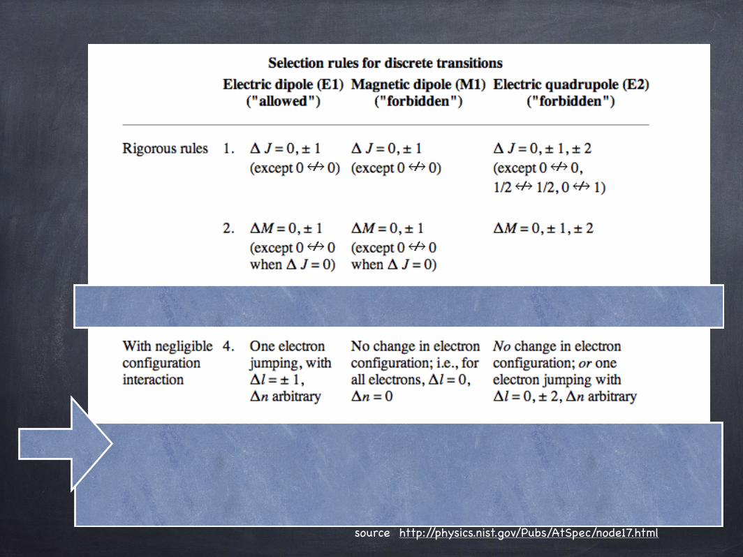
Selection rules (LS coupling)
Text
source http://physics.nist.gov/Pubs/AtSpec/node17.html
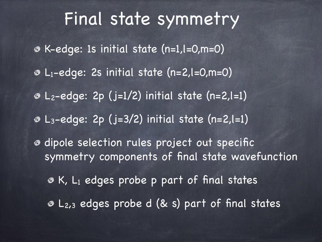
Final state symmetryK-edge: 1s initial state (n=1,l=0,m=0)
L1-edge: 2s initial state (n=2,l=0,m=0)
L2-edge: 2p (j=1/2) initial state (n=2,l=1)
L3-edge: 2p (j=3/2) initial state (n=2,l=1)
dipole selection rules project out specific symmetry components of final state wavefunction
K, L1 edges probe p part of final states
L2,3 edges probe d (& s) part of final states

The measured spectrum is a ensemble average of the “snapshot” spectra (~10-15 sec) of all the atoms of the selected type that are probed by the x-ray beam
In general, XAFS determines the statistical properties of the distribution of atoms relative to the central absorbers. In the case of single scattering the pair correlation function is probed. Multiple scattering gives information on higher order correlations. This information is encoded in the chi function:
µ(E) = µ0(E)(1+c(E)); c(E) = µ(E)�µ0(E)µ0(E)

EXAFS oscillations
Modulations in chi encode information about the local structure
chi function represents the fractional change in the absorption coefficient that is due to the presence of neighboring atoms
µ(E) = µ0(E)(1+c(E)); c(E) = µ(E)�µ0(E)µ0(E)
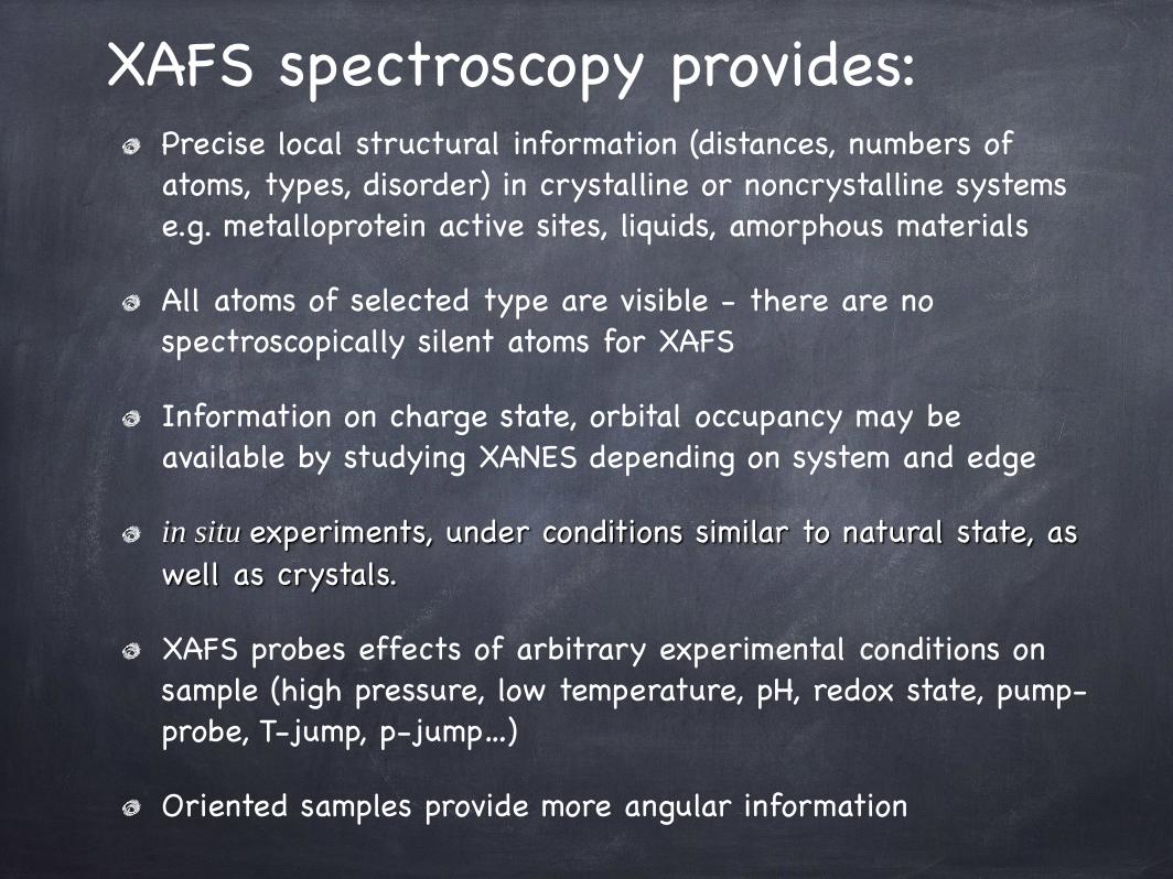
XAFS spectroscopy provides:Precise local structural information (distances, numbers of atoms, types, disorder) in crystalline or noncrystalline systems e.g. metalloprotein active sites, liquids, amorphous materials
All atoms of selected type are visible - there are no spectroscopically silent atoms for XAFS
Information on charge state, orbital occupancy may be available by studying XANES depending on system and edge
in situ experiments, under conditions similar to natural state, as well as crystals.
XAFS probes effects of arbitrary experimental conditions on sample (high pressure, low temperature, pH, redox state, pump-probe, T-jump, p-jump…)
Oriented samples provide more angular information
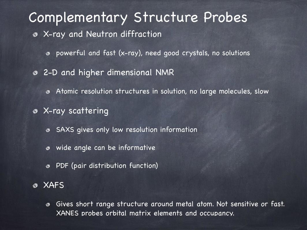
Complementary Structure ProbesX-ray and Neutron diffraction
powerful and fast (x-ray), need good crystals, no solutions
2-D and higher dimensional NMR
Atomic resolution structures in solution, no large molecules, slow
X-ray scattering
SAXS gives only low resolution information
wide angle can be informative
PDF (pair distribution function)
XAFS
Gives short range structure around metal atom. Not sensitive or fast. XANES probes orbital matrix elements and occupancy.

Related techniquesXMCD: X-ray Magnetic Circular Dichroism uses circularly polarized x-rays to probe magnetic structure
IXS: Inelastic X-ray Scattering analyzes the fluorescence radiation at high resolution, providing a 2-D excitation map. Provides a great deal of information in the near-edge region
X-ray Raman: essentially allows one to obtain XAFS-like information using high energy x-rays
DAFS: hybrid diffraction/XAFS gives sensitivity to inequivalent sites in crystals and multilayers
XPS, ARPEFS, fluorescence holography...

Single Scattering EXAFS EquationStern, Sayers, Lytle
The k-dependence of scattering amplitudes and phases helps distinguish types of backscatterers.
This equation is a bit too simple {large disorder, multiple scattering [focussing effect]}, but it can be generalized.
Experimental data are fit using the EXAFS equationwith theoretically calculated (or empirically measured)
scattering functions to determine structural parameters.
�(k) = S20
X
j
Nj
kR2j
e�2k2�2j e�2Rj/�(k)fj(k;Rj) sin (2kRj + �j(k;Rj))

k-dependence of scattering amplitudes and phases helps identify scatterers
Te
Se
S
O
0 5 10 15 200.00
0.05
0.10
0.15
0.20
k HÅ-1L
k*AHkL
k*AHkL for electron scatteringFe-O,Fe-S,Fe-Se,Fe-Te
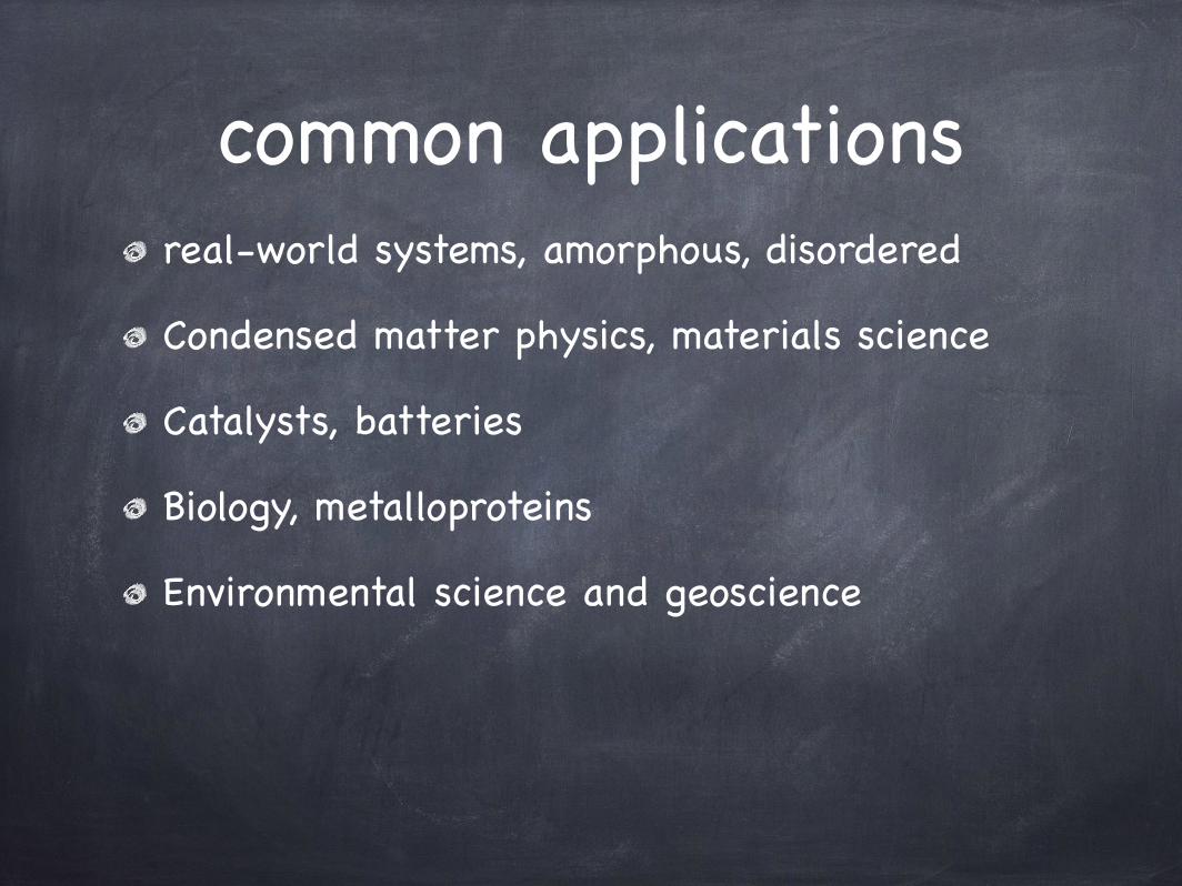
common applicationsreal-world systems, amorphous, disordered
Condensed matter physics, materials science
Catalysts, batteries
Biology, metalloproteins
Environmental science and geoscience
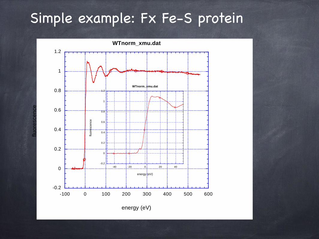
Simple example: Fx Fe-S protein
-0.2
0
0.2
0.4
0.6
0.8
1
1.2
-100 0 100 200 300 400 500 600
WTnorm_xmu.datflu
ores
cenc
e
energy (eV)
-0.2
0
0.2
0.4
0.6
0.8
1
1.2
-40 -20 0 20 40
WTnorm_xmu.datflu
ores
cenc
e
energy (eV)
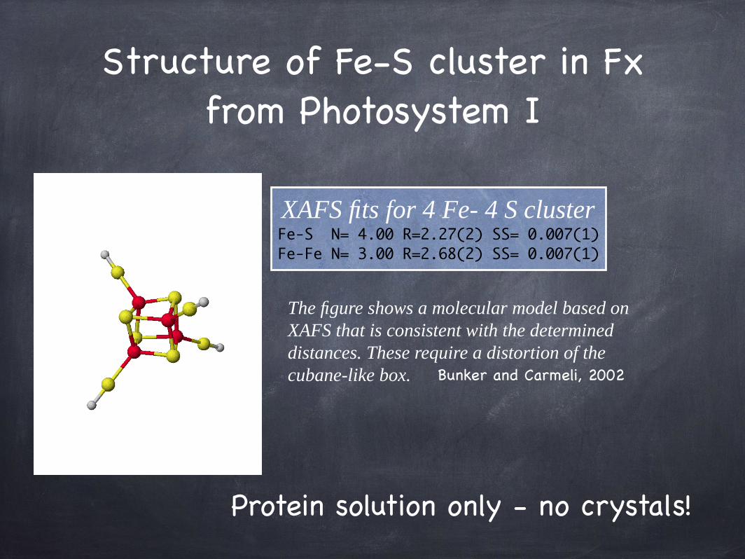
Structure of Fe-S cluster in Fx from Photosystem I
XAFS fits for 4 Fe- 4 S cluster Fe-S N= 4.00 R=2.27(2) SS= 0.007(1)Fe-Fe N= 3.00 R=2.68(2) SS= 0.007(1)
The figure shows a molecular model based on XAFS that is consistent with the determined distances. These require a distortion of the cubane-like box. Bunker and Carmeli, 2002
Protein solution only - no crystals!
Single Scattering EXAFS equation
Brief Article
The Author
August 15, 2007
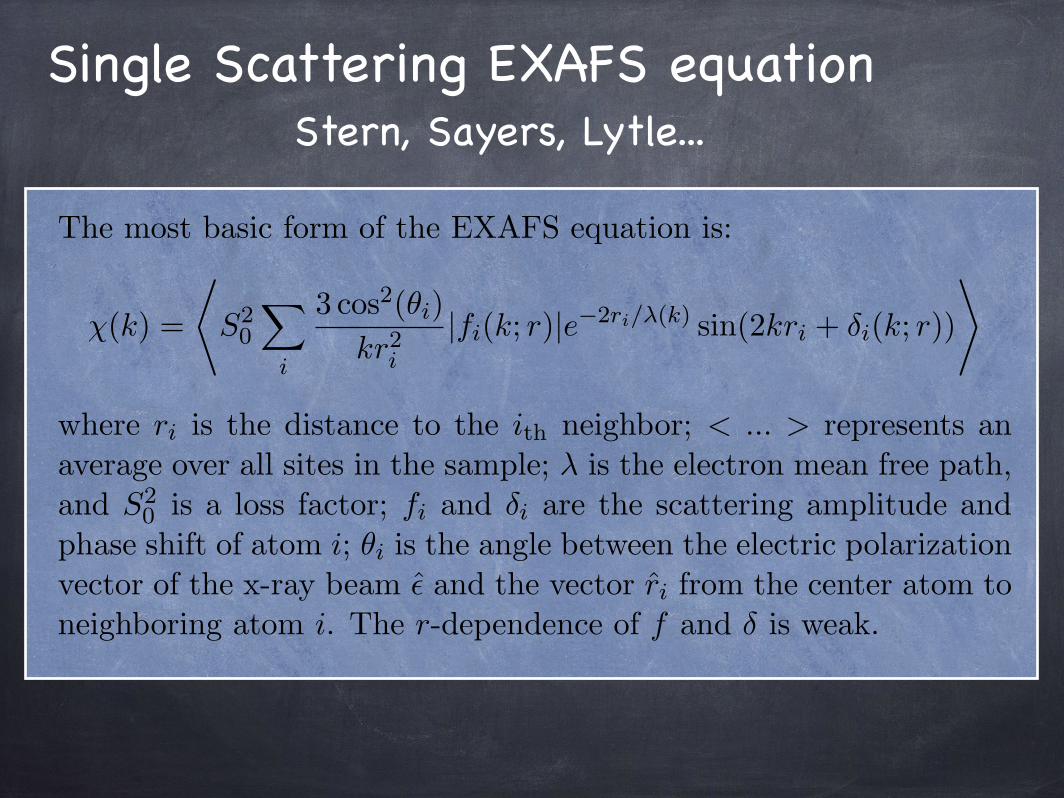
The most basic form of the EXAFS equation is:
⌃(k) =
�S2
0
⇤
i
3 cos2(⇤i)kr2
i
|fi(k; r)|e�2ri/�(k) sin(2kri + �i(k; r))
⇥
where ri is the distance to the ith neighbor; < ... > represents anaverage over all sites in the sample; ⌅ is the electron mean free path,and S2
0 is a loss factor; fi and �i are the scattering amplitude andphase shift of atom i; ⇤i is the angle between the electric polarizationvector of the x-ray beam ⇥̂ and the vector r̂i from the center atom toneighboring atom i. The r-dependence of f and � is weak.
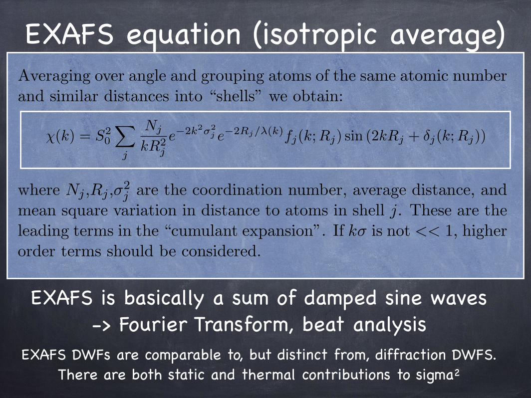
Averaging over angle and grouping atoms of the same atomic numberand similar distances into ”shells” we obtain:
⌃(k) = S20
⇤
i
Nj
kR2j
|fi(k; r)|e�2k2⇥2j e�2Rj/�(k) sin(2kRj + �j(k; r)),
where Nj ,Rj ,⇧2j are the coordination number, average distance, and
mean square variation in distance to atoms in shell j. These are theleading terms in the ”cumulant expansion”. If k⇧ is not << 1, higherorder terms should be considered.
1
Stern, Sayers, Lytle...
EXAFS equation (isotropic average)
Brief Article
The Author
August 15, 2007
The most basic form of the EXAFS equation is:
⌃(k) =
�S2
0
⇤
i
3 cos2(⇤i)kr2
i
|fi(k; r)|e�2ri/�(k) sin(2kri + �i(k; r))
⇥
where ri is the distance to the ith neighbor; < ... > represents anaverage over all sites in the sample; ⌅ is the electron mean free path,and S2
0 is a loss factor; fi and �i are the scattering amplitude andphase shift of atom i; ⇤i is the angle between the electric polarizationvector of the x-ray beam ⇥̂ and the vector r̂i from the center atom toneighboring atom i. The r-dependence of f and � is weak.
Averaging over angle and grouping atoms of the same atomic numberand similar distances into “shells” we obtain:
⌃(k) = S20
⇤
i
Nj
kR2j
|fj(k; r)|e�2k2⇥2j e�2Rj/�(k) sin(2kRj + �j(k; r)),
where Nj ,Rj ,⇧2j are the coordination number, average distance, and
mean square variation in distance to atoms in shell j. These are theleading terms in the “cumulant expansion”. If k⇧ is not << 1, higherorder terms should be considered.
1
EXAFS is basically a sum of damped sine waves-> Fourier Transform, beat analysis
EXAFS DWFs are comparable to, but distinct from, diffraction DWFS. There are both static and thermal contributions to sigma2
�(k) = S20
X
j
Nj
kR2j
e�2k2�2j e�2Rj/�(k)fj(k;Rj) sin (2kRj + �j(k;Rj))
Multiple Scattering Expansion
Brief Article
The Author
August 16, 2007
The most basic form of the EXAFS equation is:
⌥(k) =
⇧S2
0
⌥
i
3 cos2(⇤i)kr2
i
|fi(k; r)|e�2ri/⇥(k) sin(2kri + �i(k; r))
⌃
where ri is the distance to the ith neighbor; < ... > represents anaverage over all sites in the sample; ⌅ is the electron mean free path,and S2
0 is a loss factor; fi and �i are the scattering amplitude andphase shift of atom i; ⇤i is the angle between the electric polarizationvector of the x-ray beam ⇥̂ and the vector r̂i from the center atom toneighboring atom i. The r-dependence of f and � is weak.
Averaging over angle and grouping atoms of the same atomic numberand similar distances into “shells” we obtain:
⌥(k) = S20
⌥
i
Nj
kR2j
|fj(k; r)|e�2k2⌅2j e�2Rj/⇥(k) sin(2kRj + �j(k; r)),
where Nj ,Rj ,⌃2j are the coordination number, average distance, and
mean square variation in distance to atoms in shell j. These are theleading terms in the “cumulant expansion”. If k⌃ is not << 1, higherorder terms should be considered.
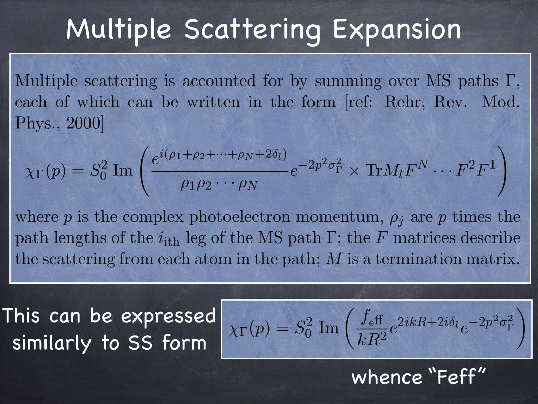
Multiple scattering is accounted for by summing over MS paths �,each of which can be written in the form [ref: Rehr, Rev. Mod.Phys., 2000]
⌥�(p) = S20 Im
⇤ei(⇤1+⇤2+···+⇤N+2�l)
⇧1⇧2 · · · ⇧Ne�2p2⌅2
� ⇥ TrMlFN · · · F 2F 1
⌅
where p is the complex photoelectron momentum, ⇧j are p times thepath lengths of the iith leg of the MS path �; the F matrices describethe scattering from each atom in the path; M is a termination matrix.
⌥�(p) = S20 Im
�fe⇥
kR2e2ikR+2i�le�2p2⌅2
�
⇥
1
This can be expressed similarly to SS form
Brief Article
The Author
August 16, 2007
The most basic form of the EXAFS equation is:
⌥(k) =
⇧S2
0
⌥
i
3 cos2(⇤i)kr2
i
|fi(k; r)|e�2ri/⇥(k) sin(2kri + �i(k; r))
⌃
where ri is the distance to the ith neighbor; < ... > represents anaverage over all sites in the sample; ⌅ is the electron mean free path,and S2
0 is a loss factor; fi and �i are the scattering amplitude andphase shift of atom i; ⇤i is the angle between the electric polarizationvector of the x-ray beam ⇥̂ and the vector r̂i from the center atom toneighboring atom i. The r-dependence of f and � is weak.
Averaging over angle and grouping atoms of the same atomic numberand similar distances into “shells” we obtain:
⌥(k) = S20
⌥
i
Nj
kR2j
|fj(k; r)|e�2k2⌅2j e�2Rj/⇥(k) sin(2kRj + �j(k; r)),
where Nj ,Rj ,⌃2j are the coordination number, average distance, and
mean square variation in distance to atoms in shell j. These are theleading terms in the “cumulant expansion”. If k⌃ is not << 1, higherorder terms should be considered.
Multiple scattering is accounted for by summing over MS paths �,each of which can be written in the form [ref: Rehr, Rev. Mod.Phys., 2000]
⌥�(p) = S20 Im
⇤ei(⇤1+⇤2+···+⇤N+2�l)
⇧1⇧2 · · · ⇧Ne�2p2⌅2
� ⇥ TrMlFN · · · F 2F 1
⌅
where p is the complex photoelectron momentum, ⇧j are p times thepath lengths of the iith leg of the MS path �; the F matrices describethe scattering from each atom in the path; M is a termination matrix.
⌥�(p) = S20 Im
�fe⇥
kR2e2ikR+2i�le�2p2⌅2
�
⇥
1 whence “Feff”
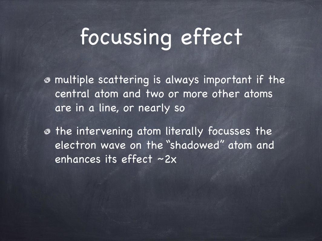
focussing effect
multiple scattering is always important if the central atom and two or more other atoms are in a line, or nearly so
the intervening atom literally focusses the electron wave on the “shadowed” atom and enhances its effect ~2x

Leading MS paths tetrahedral MnO4
reff=1.9399 reff=3.52382 reff=3.87979
reff=3.87979 reff=5.10774 reff=5.46371
2 legs 3 legs 4 legs
4 legs 4 legs 5 legs
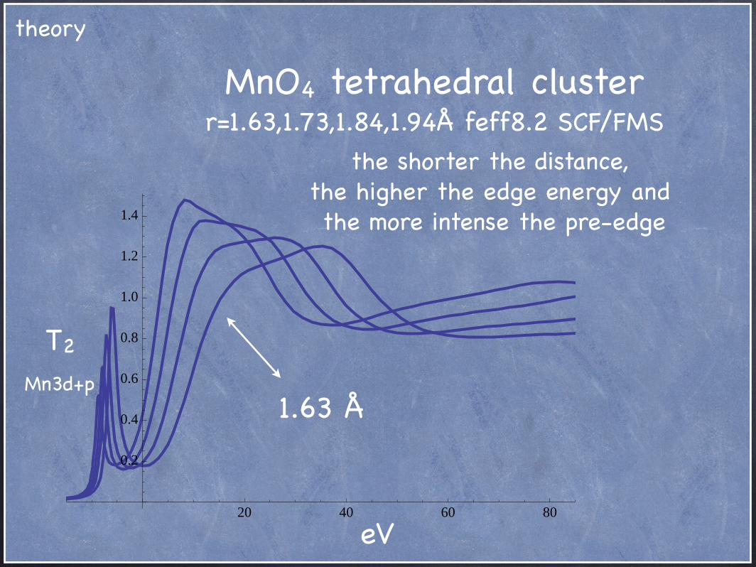
MnO4 tetrahedral cluster r=1.63,1.73,1.84,1.94Å feff8.2 SCF/FMS
eV
the shorter the distance,the higher the edge energy and the more intense the pre-edge
20 40 60 80
0.2
0.4
0.6
0.8
1.0
1.2
1.4
1.63 Å
T2
Mn3d+p
theory
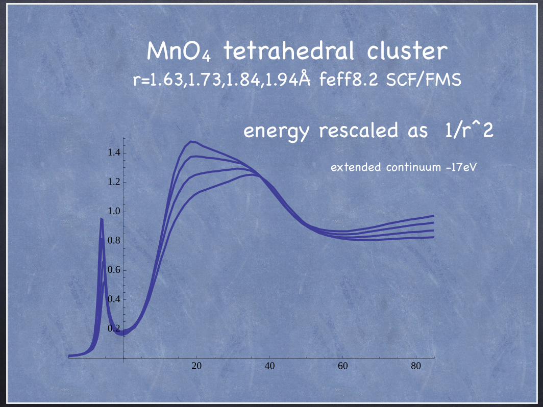
energy rescaled as 1/r^2
MnO4 tetrahedral cluster r=1.63,1.73,1.84,1.94Å feff8.2 SCF/FMS
extended continuum -17eV
20 40 60 80
0.2
0.4
0.6
0.8
1.0
1.2
1.4
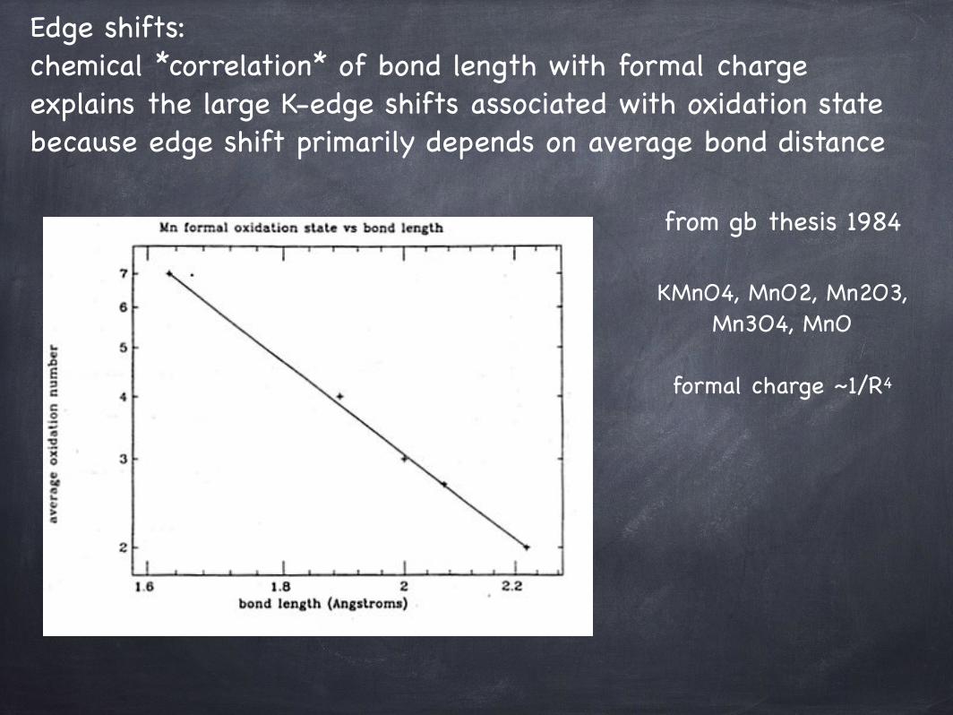
Edge shifts: chemical *correlation* of bond length with formal charge explains the large K-edge shifts associated with oxidation state because edge shift primarily depends on average bond distance
from gb thesis 1984
KMnO4, MnO2, Mn2O3, Mn3O4, MnO
formal charge ~1/R4

20 40 60 80
0.1
0.2
0.3
0.4
0.5
0.6
0.7
Solid KMnO4 at 80K and 300Kexperimental data*
the temperature sensitivefine structure over edgeis single scattering from atoms beyond first shellwith very large DWFs
* G Bunker thesis 1984
expt.

Bunker and SternPRL 52, 22 (1984)
XANES landscape is from SS+MSamong nearest neighbor tetrahedron
SS from distant atoms addstemp dependent fine structure

now for somethingcompletely different

XAFS experimental requirementssuitable sample (depends on measurement mode)
intense broad-band or scannable source
monochromatic (~ 1 eV bandwidth), scannable beam, energy suitable for elements of interest
suitable detectors (depends on mode)
special equipment (cryostats, goniometers..)
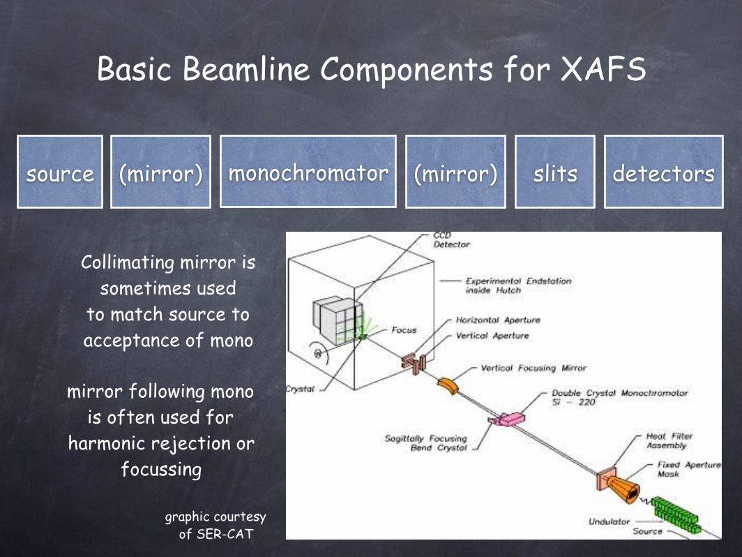
Basic Beamline Components for XAFS
(mirror)source monochromator detectorsslits(mirror)
Collimating mirror is sometimes used
to match source to acceptance of mono
mirror following mono is often used for
harmonic rejection or focussing
graphic courtesy of SER-CAT
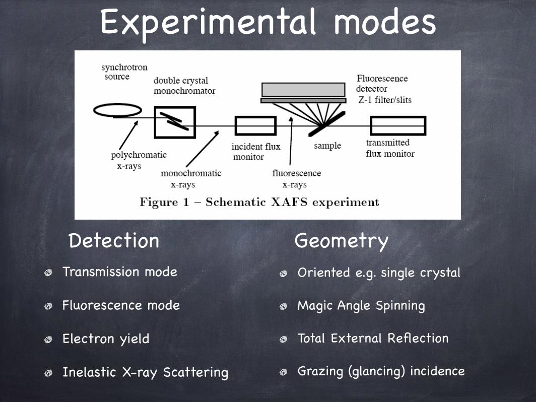
Experimental modes
Transmission mode
Fluorescence mode
Electron yield
Inelastic X-ray Scattering
Oriented e.g. single crystal
Magic Angle Spinning
Total External Reflection
Grazing (glancing) incidence
Detection Geometry
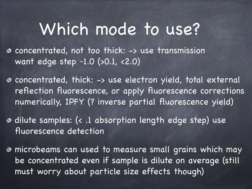
Which mode to use?concentrated, not too thick: -> use transmission want edge step ~1.0 (>0.1, <2.0)
concentrated, thick: -> use electron yield, total external reflection fluorescence, or apply fluorescence corrections numerically, IPFY (? inverse partial fluorescence yield)
dilute samples: (< .1 absorption length edge step) use fluorescence detection
microbeams can used to measure small grains which may be concentrated even if sample is dilute on average (still must worry about particle size effects though)
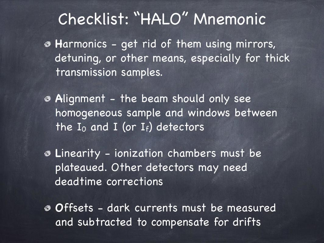
Checklist: “HALO” MnemonicHarmonics - get rid of them using mirrors, detuning, or other means, especially for thick transmission samples.
Alignment - the beam should only see homogeneous sample and windows between the I0 and I (or If) detectors
Linearity - ionization chambers must be plateaued. Other detectors may need deadtime corrections
Offsets - dark currents must be measured and subtracted to compensate for drifts
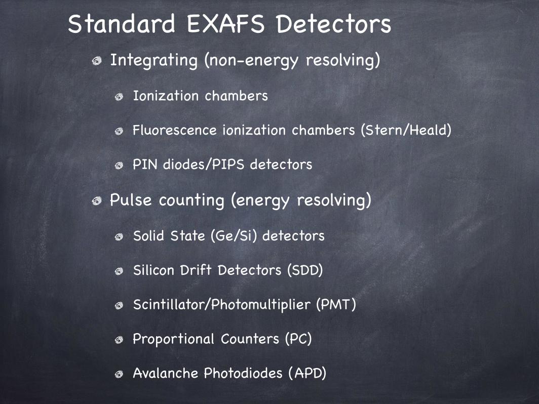
Standard EXAFS DetectorsIntegrating (non-energy resolving)
Ionization chambers
Fluorescence ionization chambers (Stern/Heald)
PIN diodes/PIPS detectors
Pulse counting (energy resolving)
Solid State (Ge/Si) detectors
Silicon Drift Detectors (SDD)
Scintillator/Photomultiplier (PMT)
Proportional Counters (PC)
Avalanche Photodiodes (APD)
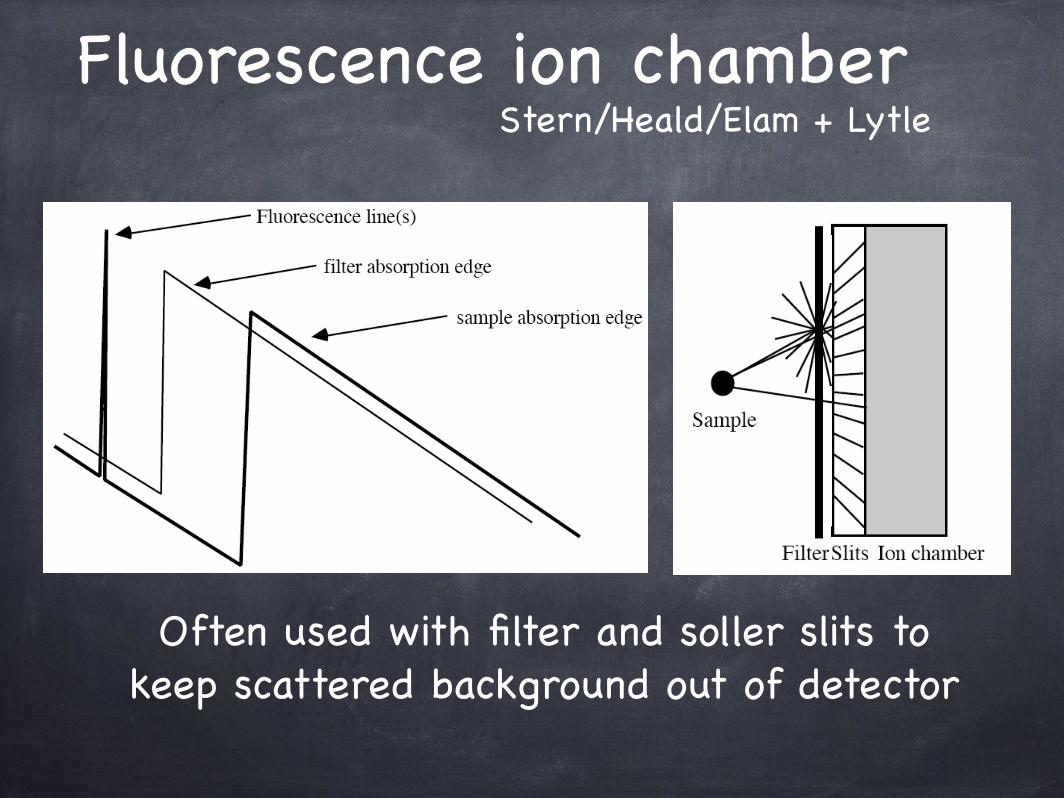
Fluorescence ion chamber
Often used with filter and soller slits to keep scattered background out of detector
Stern/Heald/Elam + Lytle

Stern/Heald/Lytle DetectorsPerformance for dilute systems depends critically on filter and
slit quality, and correct choice of filter thickness. This approach cannot eliminate fluorescence at lower energies.
for more info see: http://gbxafs.iit.edu/training/tutorials.html
excellentfilter and ideal slits
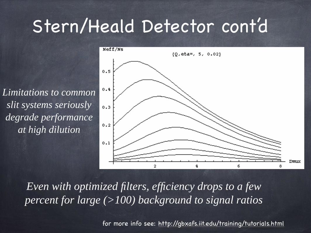
Limitations to commonslit systems seriouslydegrade performance
at high dilution
Even with optimized filters, efficiency drops to a few percent for large (>100) background to signal ratios
Stern/Heald Detector cont’d
for more info see: http://gbxafs.iit.edu/training/tutorials.html
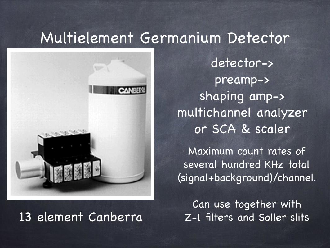
Multielement Germanium Detectordetector->preamp->
shaping amp->multichannel analyzer
or SCA & scaler
13 element Canberra
Maximum count rates of several hundred KHz total
(signal+background)/channel.
Can use together with Z-1 filters and Soller slits

SDD Arrays
77 element prototypesilicon drift detector
C. Fiorini et alTotal active area
6.7 cm^2
higher count rates are under active development
4-element high count rate silicon drift detector

X-ray AnalyzersConventional solid state detectors can be easily saturated at high flux beamlines
They spend most of their time counting background photons you throw out anyway
Multilayer, bent crystal Laue, and other analyzers eliminate background before it gets to detector
graphite log-spiral analyzer (Pease), Bragg log spiral analyzer (Attenkofer et al) are also good approaches
Effectively no count rate limits, and good collection efficiency, or better resolution
No count rate limit due to pulsed nature of source
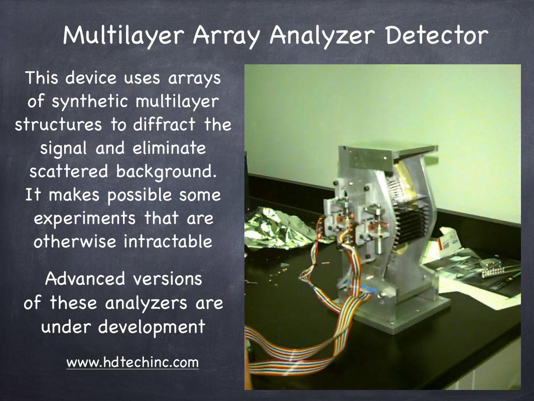
Multilayer Array Analyzer DetectorThis device uses arraysof synthetic multilayer
structures to diffract thesignal and eliminate
scattered background. It makes possible someexperiments that are otherwise intractable
Advanced versions of these analyzers are
under development
www.hdtechinc.com
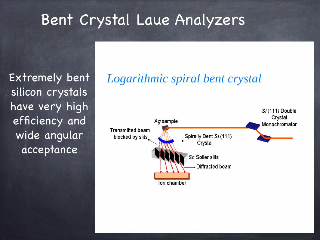
Bent Crystal Laue Analyzers
Extremely bent silicon crystalshave very highefficiency andwide angularacceptance
Logarithmic spiral bent crystal

Bent Laue Analyzer
Bent Laue Analyzer (set in bend & angle to diffract desired emission
line)
Soller Slits (matches beam divergence)
Area Integrating Detector (i.e. ionization detector)
Sample’s x-rayfluorescence

Bent Crystal Laue Analyzer
www.quercustech.com
www.fmb-oxford.com
Data AnalysisModern codes for calculating theoretical XAFS spectra are accurate enough to use to fit experimental data directly. “FEFF9” (J.J. Rehr et al) is a leading program for calculating spectra. Others include GNXAS and EXCURV.
FEFF does not analyze the data for you, however. Add-on programs of various kinds (e.g. Artemis/Athena/Horae/Demeter, Larch, Sixpack, EXAFSPAK…) use (or can use) FEFF-calculated spectra to fit the data by perturbing from an initial guess structure. Parameterizing the fitting process can be simple or quite involved.
Another approach (Dimakis & Bunker) basically uses FEFF as a subroutine and combines it with other info (e.g. DFT calculations) to estimate DWFs.
Apply instrumental Corrections (e.g. detector dead-time)Normalize data to unit edge step (compensates for sample
concentration/thickness)Convert from E -> k space (makes oscillations more uniform
spatial frequency, for BKG and Fourier transform)Subtract background using cubic splines or other methodsWeight data with kn, 1<=n<=3; (compensates for amplitude
decay)Fourier transform to distinguish shells at different distancesFourier Filter to isolate shells (optional)
Data Reduction
Data ModelingFit data in k-space, r-space, or E-space using single or
multiple scattering theory, and theoretical calculations (e.g. Feff9, GNXAS, EXCURV)
Fitting is done by describing an approximate hypothetical structure in terms of a limited number of parameters, which are adjusted to give an acceptable fit.
Good open-source software is available e.g. feff6 (Rehr), ifeffit/Artemis/Athena (Ravel/Newville), SixPack (Webb) GNXAS (Di Cicco/Filliponi), RoundMidnight(Michalowicz), EXAFSPAK (George)...
FEFF9 must be licensed, but it’s at reasonable cost.Other programs e.g. Mathematica, R can be useful.
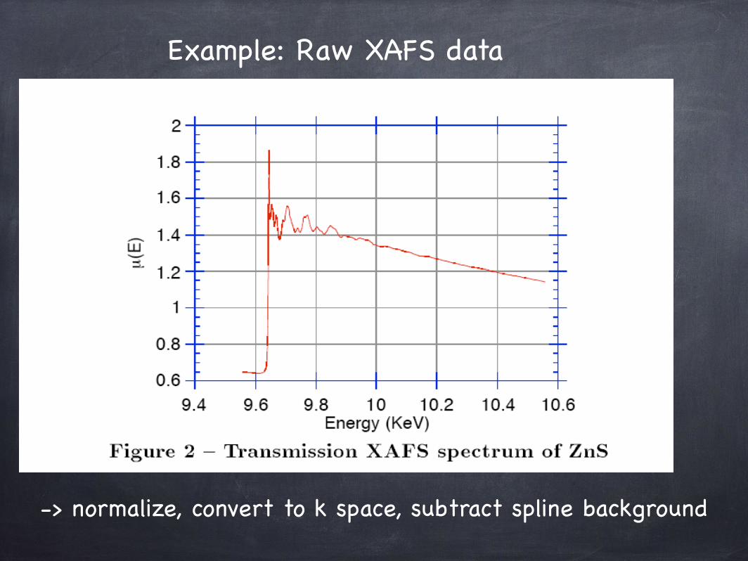
Example: Raw XAFS data
-> normalize, convert to k space, subtract spline background
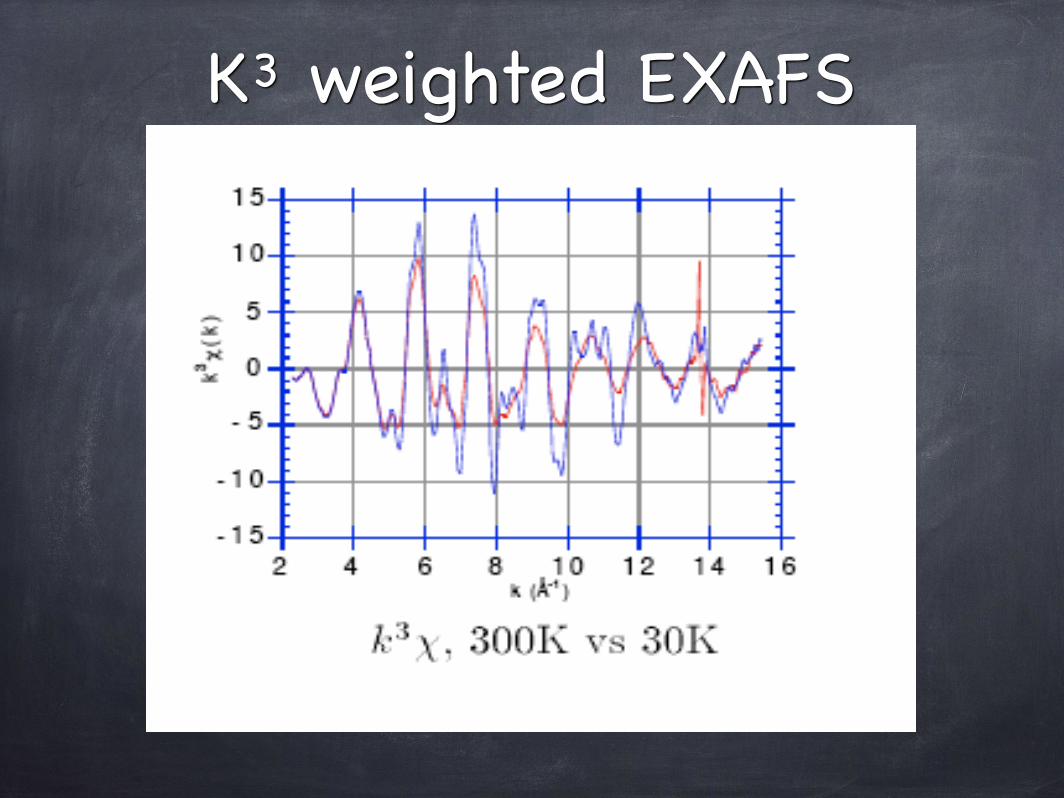
K3 weighted EXAFS
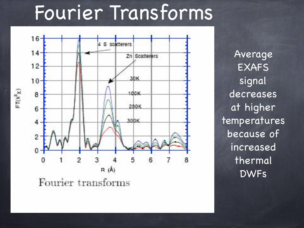
Fourier Transforms
Average EXAFSsignal
decreasesat higher
temperaturesbecause of increasedthermal DWFs

Fourier Filtered First Shell
determine single shell’s
amplitude and phase from real and imaginary parts of
inverse FT
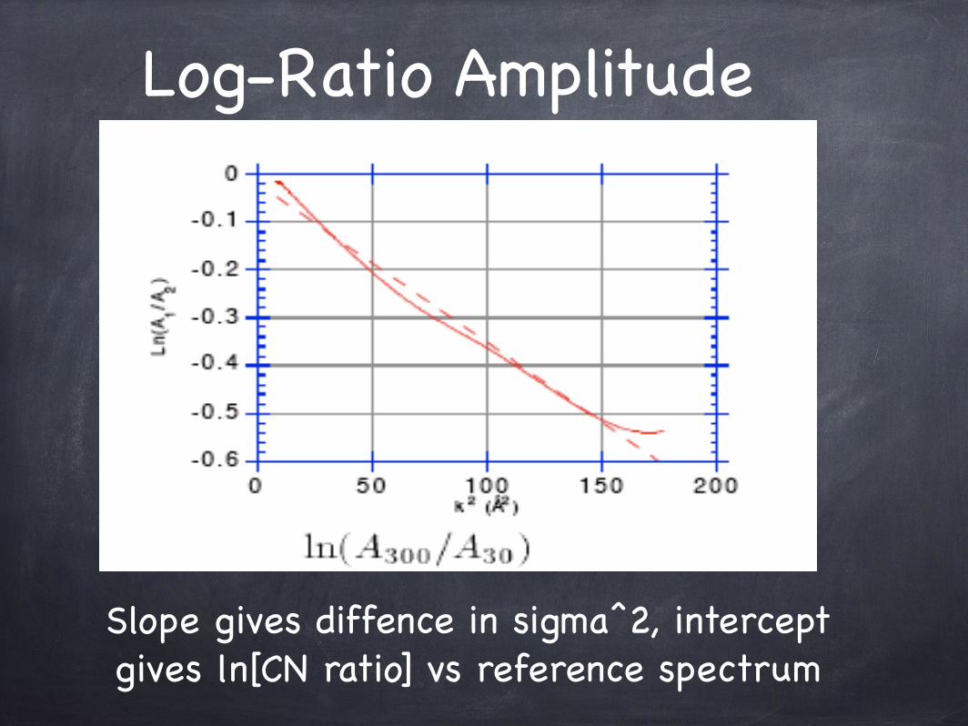
Log-Ratio Amplitude
Slope gives diffence in sigma^2, intercept gives ln[CN ratio] vs reference spectrum
Single Scattering fittingIf SS is a good approximation, and shells are well isolated, you can fit shell by shell
Complications still occur because of large disorder, accidental cancellations, and high correlation between fitting parameters
Multishell fits in SS approximation
Multiple scattering fittingMS often cannot be neglected (e.g. focussing effect)
MS fitting introduces a host of complications but also potential advantages
SS contains no information about bond angles
MS does contain bond angle information (3-body and higher correlations)
Parameter explosion -> how to handle DWFs?
Dangers of garbage-in, garbage-out
(more on this later in the talk)
TheoryImproved Theory and Practical Implementations
Fast sophisticated electron multiple scattering codes
Still limitations in near-edge (XANES) region
Solves the forward problem (structure->spectrum), but not the inverse problem (spectrum -> structure),
More work on better fitting direct methods is needed
Sophisticated quantum chemistry codes have been made easier to use; they can be leveraged to combine DFT and XAFS
correlate electronic and vibrational structure
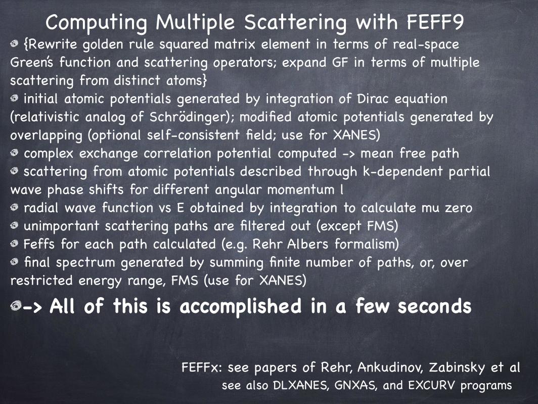
Computing Multiple Scattering with FEFF9 {Rewrite golden rule squared matrix element in terms of real-space
Green’s function and scattering operators; expand GF in terms of multiple scattering from distinct atoms} initial atomic potentials generated by integration of Dirac equation
(relativistic analog of Schrödinger); modified atomic potentials generated by overlapping (optional self-consistent field; use for XANES) complex exchange correlation potential computed -> mean free path scattering from atomic potentials described through k-dependent partial
wave phase shifts for different angular momentum l radial wave function vs E obtained by integration to calculate mu zero unimportant scattering paths are filtered out (except FMS) Feffs for each path calculated (e.g. Rehr Albers formalism) final spectrum generated by summing finite number of paths, or, over
restricted energy range, FMS (use for XANES)
-> All of this is accomplished in a few seconds
FEFFx: see papers of Rehr, Ankudinov, Zabinsky et al see also DLXANES, GNXAS, and EXCURV programs

Example: Multiple Scatteringwithin Histidine Imidazole Ring
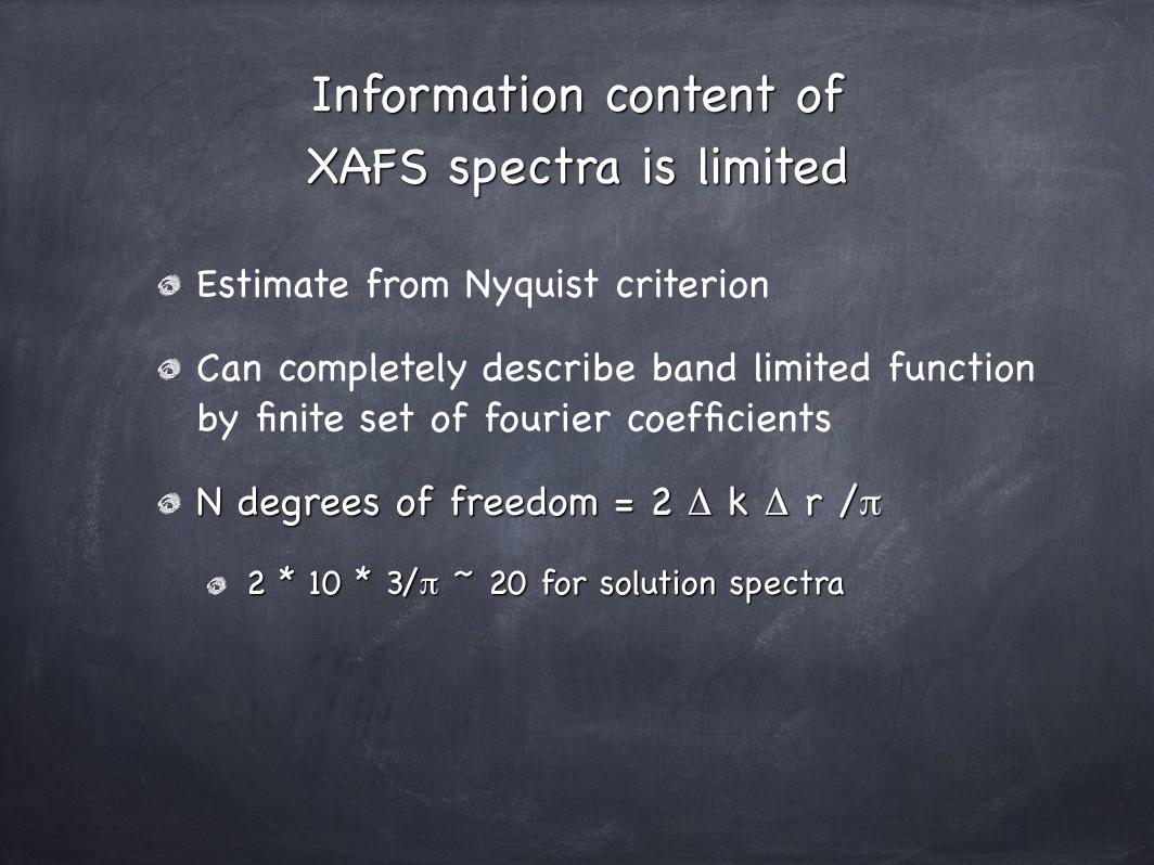
Information content of XAFS spectra is limited
Estimate from Nyquist criterion
Can completely describe band limited function by finite set of fourier coefficients
N degrees of freedom = 2 Δ k Δ r /π
2 * 10 * 3/π ~ 20 for solution spectra

Parameter explosion in MS fitting
Multiple scattering expansion
May be tens or hundreds of important paths
Each path has degeneracy, pathlength, debye waller factor, …
Geometry allows you to interrelate the pathlengths within certain limits
Group fitting (Hodgson & Co)
Determining all the MS Debye Waller parameters by fitting is a hopeless task
What can you do?
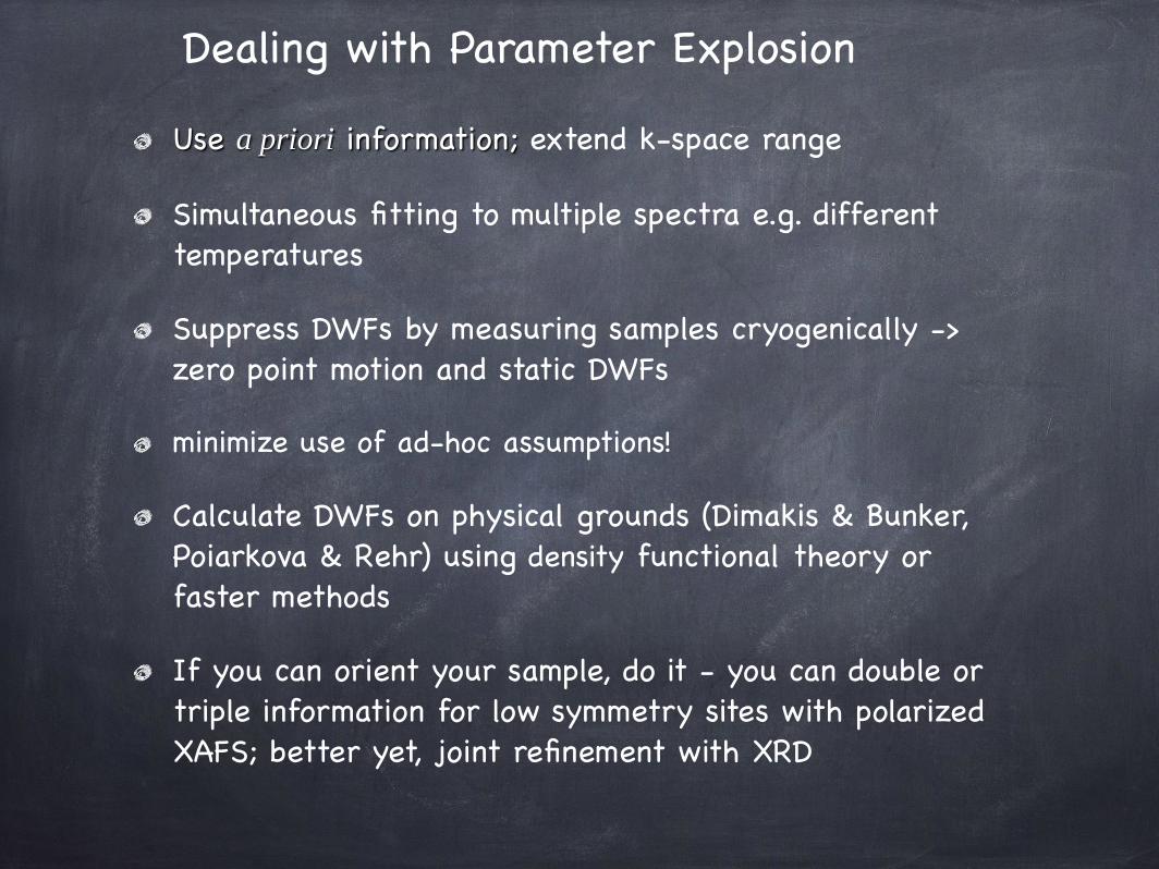
Dealing with Parameter Explosion
Use a priori information; extend k-space range
Simultaneous fitting to multiple spectra e.g. different temperatures
Suppress DWFs by measuring samples cryogenically -> zero point motion and static DWFs
minimize use of ad-hoc assumptions!
Calculate DWFs on physical grounds (Dimakis & Bunker, Poiarkova & Rehr) using density functional theory or faster methods
If you can orient your sample, do it - you can double or triple information for low symmetry sites with polarized XAFS; better yet, joint refinement with XRD
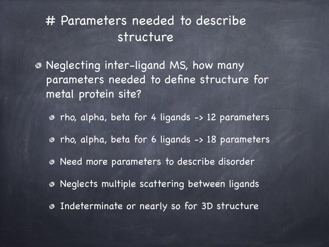
# Parameters needed to describe structure
Neglecting inter-ligand MS, how many parameters needed to define structure for metal protein site?
rho, alpha, beta for 4 ligands -> 12 parameters
rho, alpha, beta for 6 ligands -> 18 parameters
Need more parameters to describe disorder
Neglects multiple scattering between ligands
Indeterminate or nearly so for 3D structure

Polarized XAFS helpsSecond rank tensor – 3 by 3 matrix - 9 components, each a function of energy
Diagonalize to 3 independent functions
Isotropic average in solution (and cubic symmetry) to one independent function – the usual XAFS
Low symmetry structures – can get up to 3 times the information (~60 parameters) from polarized XAFS
Can use crystals that are not perfect enough for atomic resolution diffraction
In principle could solve for 3D active site structure in crystal
Joint refinement: crystallography and XAFS
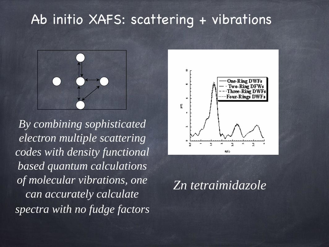
Ab initio XAFS: scattering + vibrations
By combining sophisticatedelectron multiple scattering
codes with density functional based quantum calculations of molecular vibrations, one
can accurately calculatespectra with no fudge factors
Zn tetraimidazole

His(3),Cys(1)
Zn site:Automated
fittingusing a genetic
algorithm,+ FEFF7 +ab initio DWFs.
(Dimakis& Bunker,
Biophys. Lett. 2006)

Direct methods for determining radial distribution functions fromEXAFS using Projected Landweber-Friedman Regularization
Direct Methods
Khelashvili & Bunker
Chemical SpeciationMobility and toxicity of metals in the environment strongly depends on their chemical state, which can be probed in situ with XAFS
Under appropriate conditions, the total absorption coefficient is linear combination of constituent spectra
Use singular value decomposition, principal component analysis, and linear programming (Tannazi) methods to determine species
These deliver direct methods for determining speciation
Nonlinearities arising from particle size effects theoretically and experimentally (Tannazi & Bunker)
summaryXAFS is a powerful tool for studying the local structure in both disordered and ordered materials.
Recent advances have made the technique more powerful and flexible. Much more can be and is being done to build upon and exploit recent advances in theory, experiment, and data analysis.
for more info, see http://gbxafs.iit.edu/ and book “Introduction to X-ray Absorption Fine Structure Spectroscopy”, G. Bunker, Cambridge University Press (2010)


![SESSION I X-ray Absorption Spectroscopy of …Applications of XAFS spectroscopy in mineralogy and geochemistry [10], environmental geochemistry/chemistry [11,12], interfacial chemistry](https://static.fdocuments.us/doc/165x107/5edc78f8ad6a402d666724c2/session-i-x-ray-absorption-spectroscopy-of-applications-of-xafs-spectroscopy-in.jpg)