�������� ����� ��

WSPM: Wavelet-based statistical parametric mapping

Dimitri Van De Ville, Mohamed L. Seghier, Francois Lazeyras, ThierryBlu, Michael Unser

PII: S1053-8119(07)00513-7DOI: doi: 10.1016/j.neuroimage.2007.06.011Reference: YNIMG 4735

To appear in: NeuroImage

Received date: 16 February 2007Revised date: 23 May 2007Accepted date: 3 June 2007

Please cite this article as: Van De Ville, Dimitri, Seghier, Mohamed L., Lazeyras, Fran-cois, Blu, Thierry, Unser, Michael, WSPM: Wavelet-based statistical parametric map-ping, NeuroImage (2007), doi: 10.1016/j.neuroimage.2007.06.011

This is a PDF file of an unedited manuscript that has been accepted for publication.As a service to our customers we are providing this early version of the manuscript.The manuscript will undergo copyediting, typesetting, and review of the resulting proofbefore it is published in its final form. Please note that during the production processerrors may be discovered which could affect the content, and all legal disclaimers thatapply to the journal pertain.

ACC

EPTE

D M

ANU

SCR

IPT

ACCEPTED MANUSCRIPT

WSPM: Wavelet-based statistical parametric

mapping

Dimitri Van De Ville a,∗ Mohamed L. Seghier b

Francois Lazeyras c Thierry Blu a Michael Unser a

aBiomedical Imaging Group,Ecole Polytechnique Federale de Lausanne (EPFL),Switzerland

bWellcome Trust Centre for Neuroimaging, UCL, London, UKcDepartment of Radiology and Medical Informatics, University Hospital Geneva,

Switzerland

Abstract

Recently, we have introduced an integrated framework that combines wavelet-basedprocessing with statistical testing in the spatial domain. In this paper, we proposetwo important enhancements of the framework. First, we revisit the underlyingparadigm; i.e., that the effect of the wavelet processing can be considered as anadaptive denoising step to “improve” the parameter map, followed by a statisticaldetection procedure that takes into account the non-linear processing of the data.With an appropriate modification of the framework, we show that it is possible toreduce the bias of the method with respect to the best linear estimate, providingconservative results that are closer to the original data. Second, we propose an exten-sion of our earlier technique that compensates for the lack of shift-invariance of thewavelet transform. We demonstrate experimentally that both enhancements havea positive effect on performance. In particular, we present a reproducibility studyfor multi-session data that compares WSPM against SPM with different amountsof smoothing. The full approach is available as a toolbox, named WSPM, for theSPM2 software; it takes advantage of multiple options and features of SPM such asthe general linear model.

Key words: wavelets, wavelet thresholding, statistical testing, bias reduction,shift-invariant transform, reproducibility study

∗ Corresponding author. Telephone +41-21-6935142. Fax +41-21-6933701.Email addresses: Dimitri.VanDeVille@epfl.ch (Dimitri Van De Ville),

m.seghier@fil.ion.ucl.ac.uk (Mohamed L. Seghier),Francois.Lazeyras@sim.hcuge.ch (Francois Lazeyras), Thierry.Blu@epfl.ch(Thierry Blu), Michael.Unser@epfl.ch (Michael Unser).

Preprint submitted to Elsevier Science 23 May 2007

ACC

EPTE

D M

ANU

SCR

IPT

ACCEPTED MANUSCRIPTSubmitted to NeuroImage

1 Introduction

Statistical Parametric Mapping (SPM) (Friston et al. (1995); Frackowiak et al.(1997)) is probably the most popular parametric hypothesis-driven methodfor the analysis of fMRI data. To control the multiple testing problem, SPMconsiders the data as a lattice representation of a continuous Gaussian RandomField (GRF). To conform with this hypothesis, the data is pre-smoothed witha Gaussian filter with fixed size (Worsley et al. (1996); Poline et al. (1997)).The user has the option to adjust the smoothing strength for optimal detection(compromise between SNR enhancement and spatial definition).

The discrete wavelet transform (DWT) has also been applied to the analysisof fMRI data for parametric hypothesis testing. Three important propertiesjustify the use of wavelets in this application. First, they typically encodeactivation patterns with a small set of wavelet coefficients; this is referredto as the DWT’s sparsity property. Second, an orthogonal DWT leaves thenoise evenly distributed in the wavelet domain; it therefore increases the SNR.Third, the DWT acts (approximately) as a decorrelator. Therefore, a conserva-tive Bonferroni correction for multiple hypothesis testing is closer to optimalin the wavelet domain than in the spatial domain. Basically, the standardwavelet approach to parametric hypothesis testing consists in statistical test-ing the wavelet domain representation of the parameter map (Ruttimann et al.(1998); Turkheimer et al. (2000)). The remaining difficulty is how to fully ex-ploit the reconstruction of the parameter map after thresholding in the waveletdomain. Several approaches have been proposed, such as variance reconstruc-tion or estimation of the residual in the spatial domain (Desco et al. (2005);Aston et al. (2005)), Bayesian modelling (Turkheimer et al. (2006); Flandinand Penny (2007)), optimizing statistical power while controlling false dis-covery rate (Sendur et al. (2005); Srikanth et al. (2006)), or considering thewavelet processing as a alternative preprocessing step (Wink and Roerdink(2004)). Recently, we have proposed a variation of the wavelet-based frame-work (WSPM) that performs the model-fitting and processing in the waveletdomain, but transfers the statistical testing back into the spatial domain (VanDe Ville et al. (2004)).

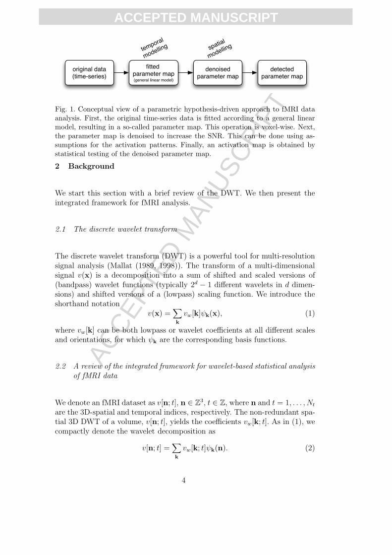
Most parametric hypothesis-driven approaches that have been proposed so farfall within the general conceptual framework that is summarized in Fig. 1. InSPM, the initial smoothing with a Gaussian filter can be seen as a denoisingprocedure to increase the SNR of the data. The subsequent detection pro-cedure is applied on the parameter map obtained from the smoothed datausing the GLM; it is based on GRF theory. The temporal processing by the

2

ACC

EPTE

D M

ANU

SCR

IPT

ACCEPTED MANUSCRIPTGLM and the spatial processing by the Gaussian filter are both linear andseparable (time × space) operations and therefore can be interchanged; i.e.,SPM’s parameter map can also be obtained by filtering the parameter mapobtained from unsmoothed data. In our wavelet-based framework, we can alsoseparate the different processing steps according to Fig. 1: temporal modellingby the GLM followed by (non-linear) denoising in the wavelet domain. Thesubsequent statistical testing takes into account the influence of the waveletprocessing but remains in the spatial domain, which has obvious advantages.

In this paper, we further investigate and extend the integrated WSPM frame-work in two important aspects:

(1) Reduction of spatial bias: Although the framework takes into accountthe statistical effect of denoising, it can still manifest spatial bias. Forinstance, weak activations in the parameter map may resemble the un-derlying pattern poorly if only a limited subset of wavelet coefficientsis retained. Notice that a similar effect can be observed with SPM: thedata is denoised by the Gaussian filtering and so is the parameter mapas well, which potentially introduces spatial bias. We extend the waveletframework to reduce this effect. Consequently, the final detected param-eter map can be considered as more closely related to the measured datawith respect to spatial bias.

(2) Better shift-invariance: The fact that the DWT is shift-variant is oftenrecognized as a major disadvantage. We show how to incorporate resultsof multiple non-redundant DWTs, for different shifts of the data, whichessentially makes the analysis shift-invariant.

The proposed framework has been integrated into SPM2 as a “WSPM tool-box”, allowing the user to have the usual SPM-based analysis and the wavelet-based framework side by side. With respect to temporal domain modelling,the full GLM fitting as provided by SPM (including compensation for serialcorrelation) is used.

In what follows, we briefly review the standard wavelet-based method, andthen introduce the enhanced framework with bias reduction and the shift-invariant extension. We illustrate and discuss the concept with several exam-ples. First, we present a 1D synthetic dataset to demonstrate the main effect ofthe proposed enhancements. Then, we analyze an experimental multi-sessiondataset using a reproducibility approach to estimate the sensitivity and speci-ficity of WSPM and SPM at different smoothing settings. We extend the typi-cal receiver-operating-characteristics (ROC) curves by a third dimension thatmeasures the bias of the methods with respect to the best-linear-unbiased es-timated of the non-smoothed data. These tri-variate plots allow us to evaluatethe trade-off that is provided by the various methods and settings.

3

ACC

EPTE

D M

ANU

SCR

IPT

ACCEPTED MANUSCRIPT

Fig. 1. Conceptual view of a parametric hypothesis-driven approach to fMRI dataanalysis. First, the original time-series data is fitted according to a general linearmodel, resulting in a so-called parameter map. This operation is voxel-wise. Next,the parameter map is denoised to increase the SNR. This can be done using as-sumptions for the activation patterns. Finally, an activation map is obtained bystatistical testing of the denoised parameter map.

2 Background

We start this section with a brief review of the DWT. We then present theintegrated framework for fMRI analysis.

2.1 The discrete wavelet transform

The discrete wavelet transform (DWT) is a powerful tool for multi-resolutionsignal analysis (Mallat (1989, 1998)). The transform of a multi-dimensionalsignal v(x) is a decomposition into a sum of shifted and scaled versions of(bandpass) wavelet functions (typically 2d − 1 different wavelets in d dimen-sions) and shifted versions of a (lowpass) scaling function. We introduce theshorthand notation

v(x) =∑k

vw[k]ψk(x), (1)

where vw[k] can be both lowpass or wavelet coefficients at all different scalesand orientations, for which ψk are the corresponding basis functions.

2.2 A review of the integrated framework for wavelet-based statistical analysis

of fMRI data

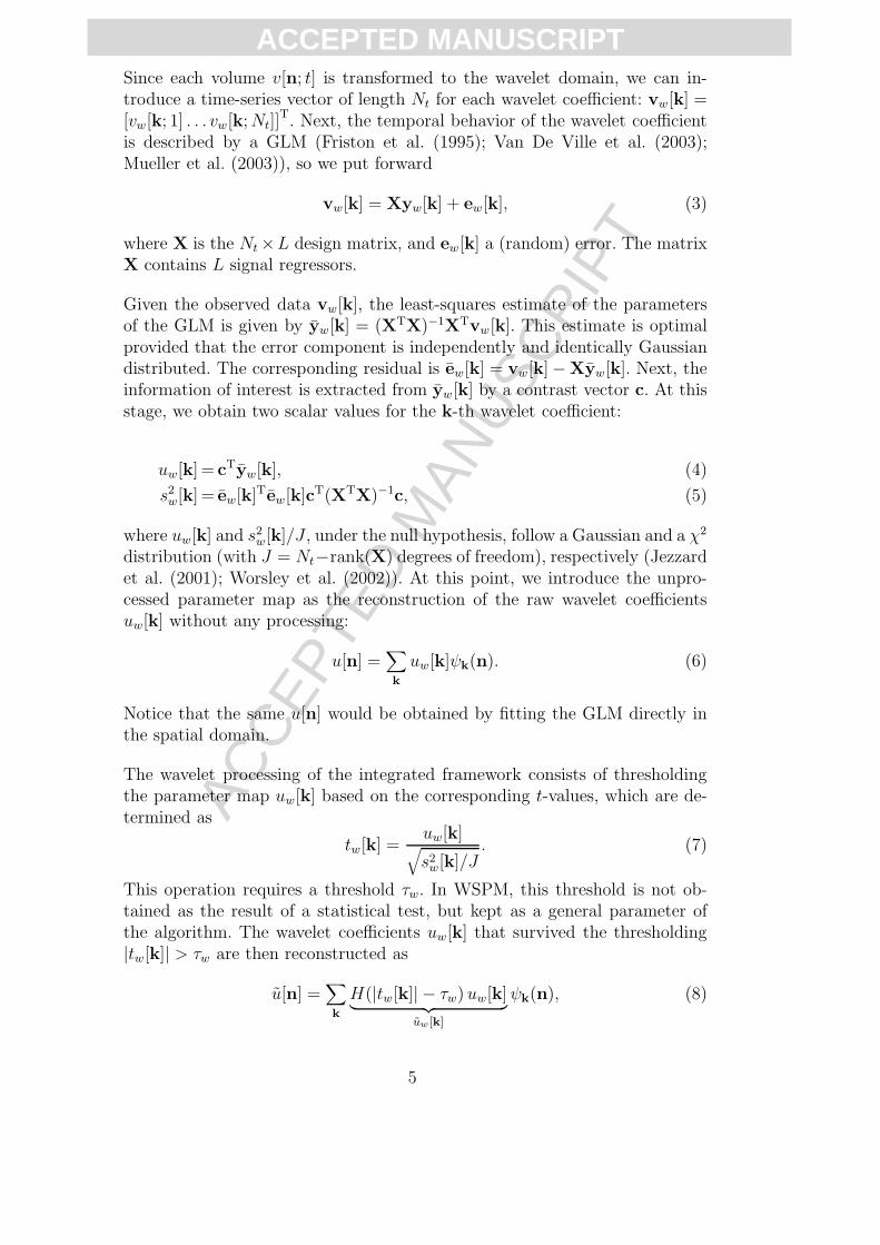
We denote an fMRI dataset as v[n; t], n ∈ Z3, t ∈ Z, where n and t = 1, . . . , Nt

are the 3D-spatial and temporal indices, respectively. The non-redundant spa-tial 3D DWT of a volume, v[n; t], yields the coefficients vw[k; t]. As in (1), wecompactly denote the wavelet decomposition as

v[n; t] =∑k

vw[k; t]ψk(n). (2)

4

ACC

EPTE

D M

ANU

SCR

IPT

ACCEPTED MANUSCRIPTSince each volume v[n; t] is transformed to the wavelet domain, we can in-troduce a time-series vector of length Nt for each wavelet coefficient: vw[k] =[vw[k; 1] . . . vw[k; Nt]]

T. Next, the temporal behavior of the wavelet coefficientis described by a GLM (Friston et al. (1995); Van De Ville et al. (2003);Mueller et al. (2003)), so we put forward

vw[k] = Xyw[k] + ew[k], (3)

where X is the Nt ×L design matrix, and ew[k] a (random) error. The matrixX contains L signal regressors.

Given the observed data vw[k], the least-squares estimate of the parametersof the GLM is given by yw[k] = (XTX)−1XTvw[k]. This estimate is optimalprovided that the error component is independently and identically Gaussiandistributed. The corresponding residual is ew[k] = vw[k] −Xyw[k]. Next, theinformation of interest is extracted from yw[k] by a contrast vector c. At thisstage, we obtain two scalar values for the k-th wavelet coefficient:

uw[k] = cTyw[k], (4)

s2w[k] = ew[k]Tew[k]cT(XTX)−1c, (5)

where uw[k] and s2w[k]/J , under the null hypothesis, follow a Gaussian and a χ2

distribution (with J = Nt−rank(X) degrees of freedom), respectively (Jezzardet al. (2001); Worsley et al. (2002)). At this point, we introduce the unpro-cessed parameter map as the reconstruction of the raw wavelet coefficientsuw[k] without any processing:

u[n] =∑k

uw[k]ψk(n). (6)

Notice that the same u[n] would be obtained by fitting the GLM directly inthe spatial domain.

The wavelet processing of the integrated framework consists of thresholdingthe parameter map uw[k] based on the corresponding t-values, which are de-termined as

tw[k] =uw[k]√s2

w[k]/J. (7)

This operation requires a threshold τw. In WSPM, this threshold is not ob-tained as the result of a statistical test, but kept as a general parameter ofthe algorithm. The wavelet coefficients uw[k] that survived the thresholding|tw[k]| > τw are then reconstructed as

u[n] =∑k

H(|tw[k]| − τw) uw[k]︸ ︷︷ ︸uw[k]

ψk(n), (8)

5

ACC

EPTE

D M

ANU

SCR

IPT

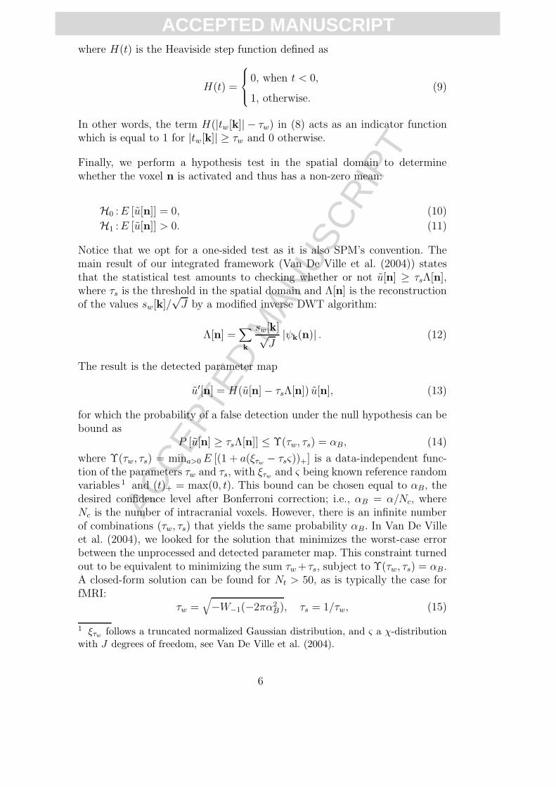
ACCEPTED MANUSCRIPTwhere H(t) is the Heaviside step function defined as

H(t) =

⎧⎪⎨⎪⎩

0, when t < 0,

1, otherwise.(9)

In other words, the term H(|tw[k]| − τw) in (8) acts as an indicator functionwhich is equal to 1 for |tw[k]| ≥ τw and 0 otherwise.

Finally, we perform a hypothesis test in the spatial domain to determinewhether the voxel n is activated and thus has a non-zero mean:

H0 : E [u[n]] = 0, (10)

H1 : E [u[n]] > 0. (11)

Notice that we opt for a one-sided test as it is also SPM’s convention. Themain result of our integrated framework (Van De Ville et al. (2004)) statesthat the statistical test amounts to checking whether or not u[n] ≥ τsΛ[n],where τs is the threshold in the spatial domain and Λ[n] is the reconstructionof the values sw[k]/

√J by a modified inverse DWT algorithm:

Λ[n] =∑k

sw[k]√J

|ψk(n)| . (12)

The result is the detected parameter map

u′[n] = H(u[n] − τsΛ[n]) u[n], (13)

for which the probability of a false detection under the null hypothesis can bebound as

P [u[n] ≥ τsΛ[n]] ≤ Υ(τw, τs) = αB, (14)

where Υ(τw, τs) = mina>0 E [(1 + a(ξτw− τsς))+] is a data-independent func-

tion of the parameters τw and τs, with ξτwand ς being known reference random

variables 1 and (t)+ = max(0, t). This bound can be chosen equal to αB, thedesired confidence level after Bonferroni correction; i.e., αB = α/Nc, whereNc is the number of intracranial voxels. However, there is an infinite numberof combinations (τw, τs) that yields the same probability αB. In Van De Villeet al. (2004), we looked for the solution that minimizes the worst-case errorbetween the unprocessed and detected parameter map. This constraint turnedout to be equivalent to minimizing the sum τw + τs, subject to Υ(τw, τs) = αB.A closed-form solution can be found for Nt > 50, as is typically the case forfMRI:

τw =√−W−1(−2πα2

B), τs = 1/τw, (15)

1 ξτwfollows a truncated normalized Gaussian distribution, and ς a χ-distribution

with J degrees of freedom, see Van De Ville et al. (2004).

6

ACC

EPTE

D M

ANU

SCR

IPT

ACCEPTED MANUSCRIPT

v[n; t] u[n]

⎧⎪⎨⎪⎩

u[n]

Λ[n]u′[n]

vw[k; t]

⎧⎪⎨⎪⎩

uw[k]

s2w[k]

⎧⎪⎪⎪⎨⎪⎪⎪⎩

uw[k]H(|tw[k]| − τw)︸ ︷︷ ︸uw[k]

sw[k]/√

J

τw τs

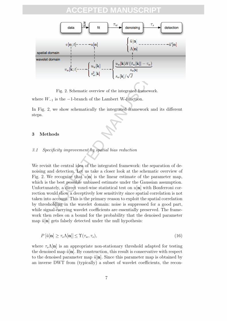
Fig. 2. Schematic overview of the integrated framework.

where W−1 is the −1-branch of the Lambert W-function.

In Fig. 2, we show schematically the integrated framework and its differentsteps.

3 Methods

3.1 Specificity improvement by spatial bias reduction

We revisit the central idea of the integrated framework: the separation of de-noising and detection. Let us take a closer look at the schematic overview ofFig. 2. We recognize that u[n] is the linear estimate of the parameter map,which is the best possible unbiased estimate under the Gaussian assumption.Unfortunately, a direct voxel-wise statistical test on u[n] with Bonferroni cor-rection would show a deceptively low sensitivity since spatial correlation is nottaken into account. This is the primary reason to exploit the spatial correlationby thresholding in the wavelet domain: noise is suppressed for a good part,while signal-carrying wavelet coefficients are essentially preserved. The frame-work then relies on a bound for the probability that the denoised parametermap u[n] gets falsely detected under the null hypothesis:

P [u[n] ≥ τsΛ[n]]≤Υ(τw, τs), (16)

where τsΛ[n] is an appropriate non-stationary threshold adapted for testingthe denoised map u[n]. By construction, this result is conservative with respectto the denoised parameter map u[n]. Since this parameter map is obtained byan inverse DWT from (typically) a subset of wavelet coefficients, the recon-

7

ACC

EPTE

D M

ANU

SCR

IPT

ACCEPTED MANUSCRIPTstruction can be spatially biased by the synthesis process.

We first recall that checking (16) corresponds to a one-sided test; i.e., largervalues of u[n] increase the probability of detection. With this in mind, we pro-pose to construct an improved parameter map u[n] out of u[n] with reducedspatial bias. We opt for a conservative point-of-view; i.e., we want to correctfor the case when the parameter is overestimated by the reconstruction afterthresholding in the wavelet domain. This typically arises when the threshold-ing operation keeps isolated wavelet coefficients in which case the secondaryripples of the wavelet function may survive spatial thresholding (“ringing” ef-fect). Therefore, we compare the denoised map u[n] against the linear estimateu[n], and we construct the corrected map as

u[n] =min(u[n], u[n]) ≤ u[n]. (17)

Basically, this means that we do only follow the denoised map if it is nothigher than the linear estimate. Our choice could miss activations that areunderestimated by the linear approach (as the denoised map will be correctedaccordingly). However, the linear estimate is unbiased and we believe thatspatial bias introduced by the basis functions is important to compensate for.

The conservativeness of the spatial bias reduction (17) follows from u[n] beingobviously closer to u[n] than u[n] is; i.e., ||u − u|| ≤ ||u − u||. Because u[n] ≤u[n], we automatically have that u[n] ≥ τsΛ[n] also implies u[n] ≥ τsΛ[n].Consequently, we have

P [u[n] ≥ τsΛ[n]] ≤ P [u[n] ≥ τsΛ[n]] , (18)

which, in turn, is upper bounded by Υ(τw, τs). We can thus perform the sametest on u[n] as we did on u[n], with the same bound. Finally, the detectedparameter map becomes

u′[n] = H(u[n] − τsΛ[n]) u[n]. (19)

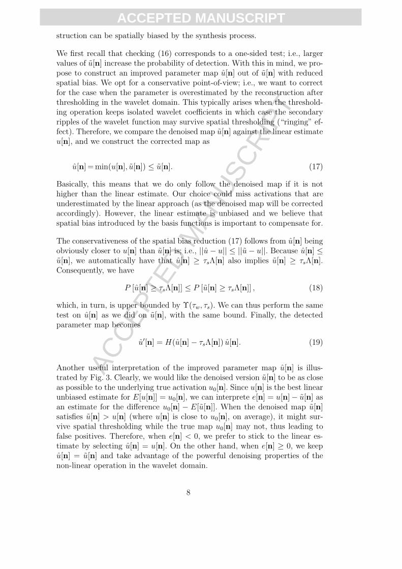
Another useful interpretation of the improved parameter map u[n] is illus-trated by Fig. 3. Clearly, we would like the denoised version u[n] to be as closeas possible to the underlying true activation u0[n]. Since u[n] is the best linearunbiased estimate for E[u[n]] = u0[n], we can interprete e[n] = u[n]− u[n] asan estimate for the difference u0[n] − E[u[n]]. When the denoised map u[n]satisfies u[n] > u[n] (where u[n] is close to u0[n], on average), it might sur-vive spatial thresholding while the true map u0[n] may not, thus leading tofalse positives. Therefore, when e[n] < 0, we prefer to stick to the linear es-timate by selecting u[n] = u[n]. On the other hand, when e[n] ≥ 0, we keepu[n] = u[n] and take advantage of the powerful denoising properties of thenon-linear operation in the wavelet domain.

8

ACC

EPTE

D M

ANU

SCR

IPT

ACCEPTED MANUSCRIPT

u0[n] v[n; t] u[n] u[n] u[n] u′[n]

Fig. 3. The denoising procedure of the integrated framework has been extended toobtain a parameter map u[n] after denoising and bias reduction.

We recall that the framework is characterized by the two threshold values τw

and τs. For the original framework, we showed that minimizing the worst-casedifference between the linear fit u[n] and the detected parameter map u′[n],corresponds to minimizing the sum τw + τs. For the extended framework,we ask a similar question, but this time for the new end-to-end difference|u[n] − u′[n]|. By expressing this difference as

|u[n] − u′[n]|= |u[n] − u[n] + u[n] − u′[n]|≤ |u[n] − u[n]| + |u[n] − u′[n]|= |u[n] − min(u[n], u[n])| + |u[n]| (1 − H(u[n] − τsΛ[n]))

≤ |u[n] − u[n]| + τsΛ[n]

≤ (τw + τs)Λ[n],

we see that the optimal values of τw and τs remain unmodified; i.e., they areobtained by minimizing their sum subject to Υ(τw, τs) = αB.

3.2 Shift-invariant wavelet processing

One of the major disadvantages of the non-redundant DWT is its shift vari-ance; i.e., a shift of the input signal does not simply translate into a shiftof the wavelet coefficients. Consequently, shifting an activation region couldturn out to give different detected patterns. The potential of the redundant(translation-invariant) DWT has been suggested before by Turkheimer et al.(2000) in the context of direct statistical testing in the wavelet domain. At firstsight, plugging in the redundant DWT into our framework looks very temptingsince the threshold values τw and τs would remain unchanged. Unfortunately,there is a catch. Small activation regions or activations barely detected wouldbe detected by a few coefficients only, whose energy has been decreased by theredundancy factor. Therefore, the denoised parameter map would show lowervalues than in the non-redundant case (assuming the non-redundant transformis located at the “right” shift), and detection would become less sensitive.

We propose to mitigate this problem by analyzing the data under M differentshifts. The data volumes are shifted by a vector dm, m = 1, . . . , M , analyzed

9

ACC

EPTE

D M

ANU

SCR

IPT

ACCEPTED MANUSCRIPTusing the normal DWT, and the results are shifted back by −dm. That way,we obtain for each shift:

P[u(m)[n] ≥ τsΛ

(m)[n]]≤ Υ(τw, τs). (20)

We combine these results by selecting the one that results into the highestnormalized value:

P

[max

m

(u(m)[n]

Λ(m)[n]

)≥ τs

]= P

[M∨

m=1

u(m)[n] ≥ τsΛ(m)[n]

](21)

≤M∑

m=1

P[u(m)[n] ≥ τsΛ

(m)[n]]

(22)

≤MΥ(τw, τs). (23)

Clearly, the redundancy factor M increases the threshold values with respectto the non-redundant case. From this point of view, the proposed extension isnot yet completely optimal, since it does not take into account the correlationbetween the different shifted versions. Despite the higher threshold values,experimental results will show that the combinations increases sensitivity, al-though the threshold values are slightly higher.

To be fully shift-invariant with Jw decomposition levels, we need M = 22Jw

shifts in 2-D, and M = 23Jw in 3-D. They can be constructed easily by con-sidering all possible shifts 0, . . . , 2Jw in every dimension. For example, in 3-Dwe have

dm =

⎛⎜⎜⎜⎜⎜⎝

m

�m/2Jw��m/22Jw�

⎞⎟⎟⎟⎟⎟⎠ modulo 2Jw , m = 0, . . . , 23Jw . (24)

In practice, it is sufficient to keep M low and to be only shift-invariant at thefirst decomposition level; i.e., 4 when the wavelet transform is deployed in 2-Dor 8 for 3-D.

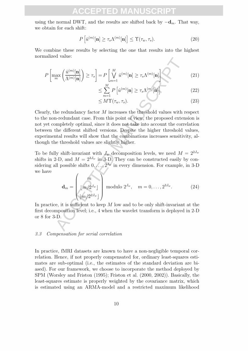
3.3 Compensation for serial correlation

In practice, fMRI datasets are known to have a non-negligible temporal cor-relation. Hence, if not properly compensated for, ordinary least-squares esti-mates are sub-optimal (i.e., the estimates of the standard deviation are bi-ased). For our framework, we choose to incorporate the method deployed bySPM (Worsley and Friston (1995); Friston et al. (2000, 2002)). Basically, theleast-squares estimate is properly weighted by the covariance matrix, whichis estimated using an ARMA-model and a restricted maximum likelihood

10

ACC

EPTE

D M

ANU

SCR

IPT

ACCEPTED MANUSCRIPT(ReML) method, which is then incorporated into the linear model to pre-whiten the data. The degrees of freedom are estimated by the Satterthwaiteapproximation (Worsley and Friston (1995)). Since the temporal model is spa-tially stationary, it can be transposed without any problem to the time-seriesof the wavelet coefficients. Whitening and parameter estimation are dealt withby functions available from SPM.

4 WSPM: A new toolbox for SPM

The extended framework has been implemented as a “WSPM toolbox” (ver-sion 1.2) for SPM2. In this way, the user can setup his experiments as usualusing SPM’s extensive features for preprocessing (e.g., registration) and GLMspecification, including the HRF modelling. Next to the standard analysis per-formed by SPM, the toolbox allows to use our framework for spatio-waveletstatistical testing. Its results are added as new “contrasts” to the SPM struc-ture related to the experiment, and they can be explored using SPM’s exten-sive features for visualization and cluster analysis. This toolbox can be freelydownloaded from http://bigwww.epfl.ch/wspm/.

5 Simulation results

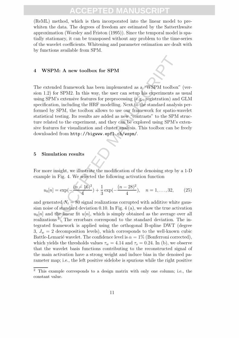
For more insight, we illustrate the modification of the denoising step by a 1-Dexample in Fig. 4. We selected the following activation function

u0[n] = exp(−(n − 16)2

4) +

1

3exp(−(n − 28)2

4), n = 1, . . . , 32, (25)

and generated Nt = 80 signal realizations corrupted with additive white gaus-sian noise of standard deviation 0.10. In Fig. 4 (a), we show the true activationu0[n] and the linear fit u[n], which is simply obtained as the average over allrealizations 2 . The errorbars correspond to the standard deviation. The in-tegrated framework is applied using the orthogonal B-spline DWT (degree3, Jw = 2 decomposition levels), which corresponds to the well-known cubicBattle-Lemarie wavelet. The confidence level is α = 1% (Bonferroni corrected),which yields the thresholds values τw = 4.14 and τs = 0.24. In (b), we observethat the wavelet basis functions contributing to the reconstructed signal ofthe main activation have a strong weight and induce bias in the denoised pa-rameter map; i.e., the left positive sidelobe is spurious while the right positive

2 This example corresponds to a design matrix with only one column; i.e., theconstant value.

11

ACC

EPTE

D M

ANU

SCR

IPT

ACCEPTED MANUSCRIPT

5 10 15 20 25 30

0.2

0

0.2

0.4

0.6

0.8

1

1

2

5 10 15 20 25 30

0.2

0

0.2

0.4

0.6

0.8

1

1

3

4

(a) (b)

5 10 15 20 25 30

0.2

0

0.2

0.4

0.6

0.8

1

1

5

4

(c)

Fig. 4. One-dimensional example to illustrate the effect of the spatial bias reductionafter the denoising step. (a) Original signal and linear estimate. (b) Non-linearestimate after adaptive denoising in the wavelet domain. (c) Non-linear estimateafter bias reduction. Legend: 1: ground truth u0; 2: linear estimate u; 3: non-linearestimate u; 4: spatial threshold τsΛ; 5: non-linear estimate with bias reduction u.

sidelobe reinforces the smaller activation. In (c), we see how the systematicovershoot (positive sidelobes) has been suppressed in the bias-reduced param-eter map u; the negative lobes are still remaining but they have no incidenceon detections, as a one-sided test is used.

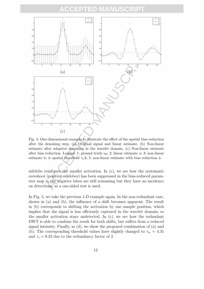
In Fig. 5, we take the previous 1-D example again. In the non-redundant case,shown in (a) and (b), the influence of a shift becomes apparent. The resultin (b) corresponds to shifting the activation by one sample position, whichimplies that the signal is less efficiently captured in the wavelet domain; sothe smaller activation stays undetected. In (c), we see how the redundantDWT is able to combine the result for both shifts, but suffers from a reducedsignal intensity. Finally, in (d), we show the proposed combination of (a) and(b). The corresponding threshold values have slightly changed to τw = 4.31and τs = 0.23 due to the redundancy factor of 2.

12

ACC

EPTE

D M

ANU

SCR

IPT

ACCEPTED MANUSCRIPT

5 10 15 20 25 30

0.2

0

0.2

0.4

0.6

0.8

1

1

5

4

5 10 15 20 25 30

0.2

0

0.2

0.4

0.6

0.8

1

1

6

4

(a) (b)

5 10 15 20 25 30

0.2

0

0.2

0.4

0.6

0.8

1

1

7

8

5 10 15 20 25 30

0.2

0

0.2

0.4

0.6

0.8

1

1

9

10

(c) (d)

Fig. 5. One-dimensional example to illustrate the effect of translation. (a) Non-lin-ear estimate for non-redundant DWT. (b) Non-linear estimate for non-redundantDWT, but signal shifted by one position. (c) Non-linear estimate for redundantDWT. (d) Combining the estimates using the non-redundant DWT. Legend: 1:ground truth u0; 4: spatial threshold τsΛ; 5: non-linear estimate u(1) using non-re-dundant DWT; 6: non-linear estimate u(2) using non-redundant DWT but withshifted signal; 7: non-linear estimate ured using the redundant DWT; 8: spatialthreshold τsΛred using the redundant DWT; 9: non-linear estimate umax combiningthe non-redundant DWTs; 10: spatial threshold τsΛmax.

6 Experimental results

In this section, we propose an evaluation of WSPM compared to SPM2, basedon real multi-session fMRI data. The dataset here comes from a carefully con-ducted experiment with auditory stimulation. All experiments were approvedby the Ethical Committee of the Geneva University Hospital.

13

ACC

EPTE

D M

ANU

SCR

IPT

ACCEPTED MANUSCRIPT6.1 Paradigm and stimuli

A block paradigm that alternates between “rest” and “stimulation” sequencesis applied. One period of the design consists of 24s of auditory stimulationfollowed by 12s of silence. The subject is exposed to single-frequency acousticstimulation, which are 0.5s sinusoidal tone bursts at a rate of 1Hz. Thesestimuli are delivered binaurally at a comfortable loudness level. Four differentfrequencies are used: 300Hz, 1126Hz, 2729Hz, and 4690Hz. A total of 4 sessionsis carried out within the same fMRI experiment, and the order of blocks ofauditory stimulation at different frequencies is permutated across sessions. Ineach session, the stimulation/silent block is repeated twice for each of the 4frequency values for a total acquisition time of about 5 minutes per session.

6.2 MRI acquisition

The MRI data is acquired on a 1.5T system (Philips Medical Systems, Best,The Netherlands). The multi-slice volume is positioned using sagittal scout im-ages. Before the functional MR scans, an anatomical scan (a GRE T1-weightedsequence, TR/TE/Flip = 162ms / 4.47ms / 80◦, FOV = 230mm, matrix =256×256, slice-thickness = 3mm) is performed to acquire the same volume asin the functional session. Functional imaging consists of an EPI GRE sequence(TR/TE/Flip = 1.2s / 40ms / 80◦, FOV = 230mm, matrix = 128 × 128, 14contiguous 3mm axial slices, spatial resolution 1.8×1.8×3mm). The exploredvolume is measured 20 times during each period of auditory stimulation and10 times during each silent period. Functional scanning is always preceded by8s of dummy scans to ensure tissue steady-state magnetization. The subject’shead is placed within a custom-designed headset with insulation, which filtersout most of the MR scanners noise (70dB attenuation for 250-8000Hz range).

6.3 Data analysis

Data processing is carried out with the Statistical Parametric Mapping SPM2software package (Wellcome Department of Imaging Neuroscience, LondonUK, http://www.fil.ion.ucl.ac.uk/spm/). All functional volumes of the 4sessions are spatially realigned to a reference functional volume. Realigned im-ages are then smoothed with an isotropic Gaussian kernel of appropriate size(FWHM). The pre-processed functional volumes of each subject are then sub-mitted to fixed-effects analysis using the general linear model (GLM) appliedat each voxel across the whole brain. Each condition of interest (i.e. auditorystimulation and silent blocks) is modelled by a boxcar waveform convolved

14

ACC

EPTE

D M

ANU

SCR

IPT

ACCEPTED MANUSCRIPTwith a canonical hæmodynamic response function (with no dispersion or tem-poral derivatives) and subjected to a multiple regression analysis with sixcovariates of no interest representing the head motion parameters, see Fristonet al. (1996a); Johnstone et al. (2006). The estimation process also includeshigh-pass filtering (1/128 Hz cutoff) to remove low-frequency noise and signaldrift, as well as AR-modeling to compensate for serial correlation.

The statistical tests with SPM are performed on the smoothed and realignedimages. Contrast volumes are computed for the main effect of auditory stim-ulation (“all frequencies”) versus silent periods over the 4 sessions. Statisticalparametric maps of the t statistics (SPMt) are obtained; these are correctedfor multiple testing based on SPM’s Gaussian Random Field theory (FWE cor-rection). To evaluate the influence of smoothing, we considered three Gaussianfilter settings: 4mm, 6mm, and 8mm FWHM (voxel size=1.8 × 1.8 × 3mm).

For the WSPM analysis, the same realigned images (but without smoothing)are decomposed using the following wavelet transforms:

• 2D orthogonal B-spline wavelet transform of degree 1.0, number of decom-position levels Jw = 1 and Jw = 2.

• 3D orthogonal B-spline wavelet transform of degree 1.0, number of decom-position levels Jw = 1 and Jw = 2.

WSPM uses simple Bonferroni correction to deal with the multiple testingproblem.

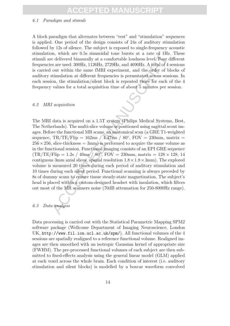
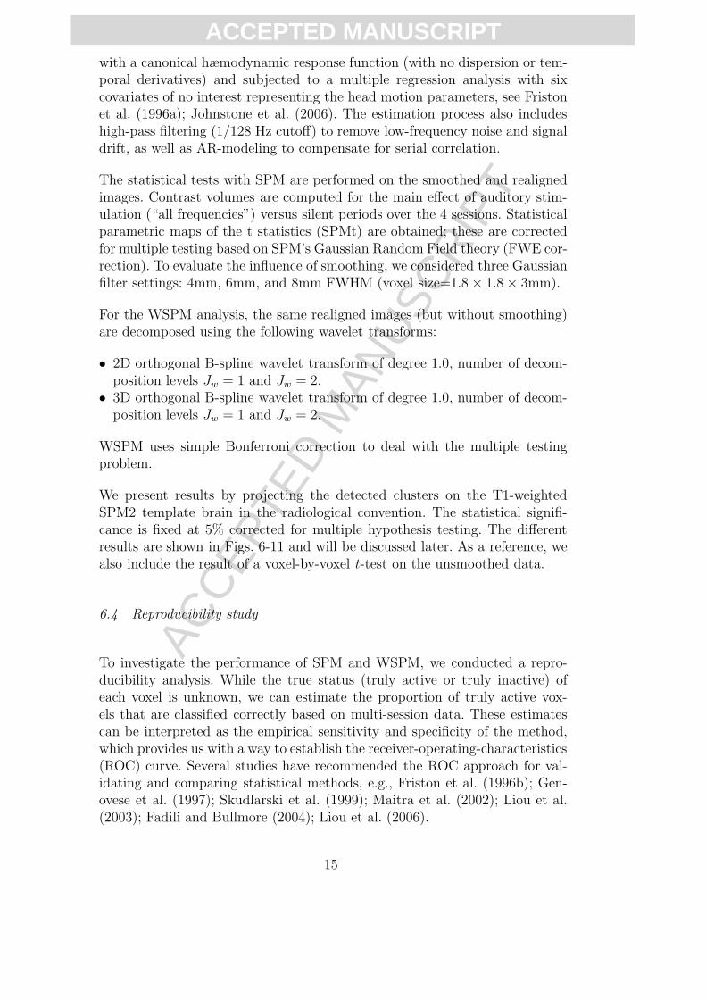
We present results by projecting the detected clusters on the T1-weightedSPM2 template brain in the radiological convention. The statistical signifi-cance is fixed at 5% corrected for multiple hypothesis testing. The differentresults are shown in Figs. 6-11 and will be discussed later. As a reference, wealso include the result of a voxel-by-voxel t-test on the unsmoothed data.

6.4 Reproducibility study

To investigate the performance of SPM and WSPM, we conducted a repro-ducibility analysis. While the true status (truly active or truly inactive) ofeach voxel is unknown, we can estimate the proportion of truly active vox-els that are classified correctly based on multi-session data. These estimatescan be interpreted as the empirical sensitivity and specificity of the method,which provides us with a way to establish the receiver-operating-characteristics(ROC) curve. Several studies have recommended the ROC approach for val-idating and comparing statistical methods, e.g., Friston et al. (1996b); Gen-ovese et al. (1997); Skudlarski et al. (1999); Maitra et al. (2002); Liou et al.(2003); Fadili and Bullmore (2004); Liou et al. (2006).

15

ACC

EPTE

D M

ANU

SCR

IPT

ACCEPTED MANUSCRIPT4mm

6mm

8mm

Fig. 6. Activation maps for the contrast “all frequencies – rest” obtained by SPMat various smoothing, 5% (FWE correction).

16

ACC

EPTE

D M

ANU

SCR

IPT

ACCEPTED MANUSCRIPT

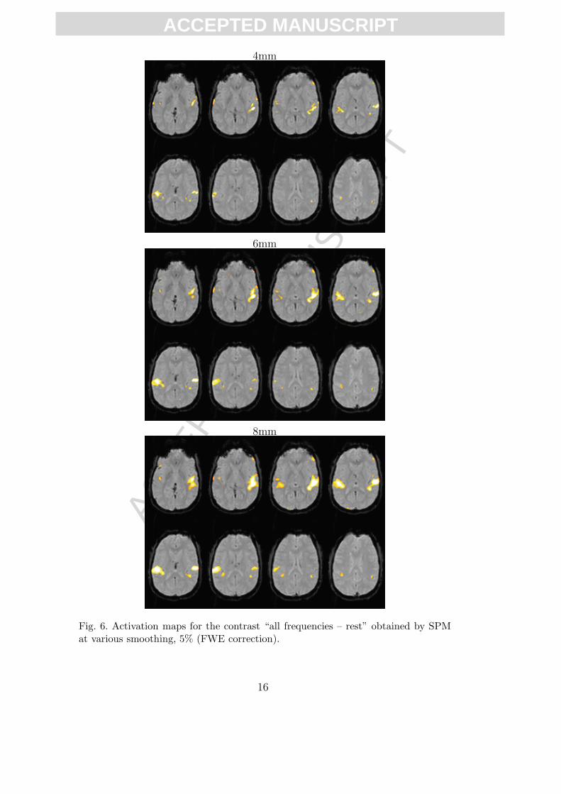
Fig. 7. Activation maps for the contrast “all frequencies – rest” obtained by voxel–wise t-test, 5%(Bonferroni corrected).

bias reduction no bias reduction

Fig. 8. Activation maps for the contrast “all frequencies – rest” obtained by WSPM,5% (Bonferroni corrected), for the 2D wavelet transform without redundancy (2decomposition levels). Left: with bias reduction; right: without bias reduction.

The main idea is to exploit the consistency in the detections over multiplesessions. To that end, we consider the cumulative sum of the individual binaryactivation maps, which takes values between 0 and K, where K is the numberof sessions. The normalized histogram of the cumulative map is denoted byq[k], k = 0, . . . , K, and considered to be a realization of a process that followsthe binomial mixture law:⎛

⎜⎝ K

k

⎞⎟⎠ [

λpk

A(1 − pA)K−k + (1 − λ)pk

I(1 − pI)K−k

], (26)

where pA and pI denote the sensitivity and false positive rate, respectively, andλ the mixture parameter that represents the proportion of truly active voxels.

17

ACC

EPTE

D M

ANU

SCR

IPT

ACCEPTED MANUSCRIPTno shift one voxel shift horizontal

one voxel shift vertical one voxel shift horizontal & vertical

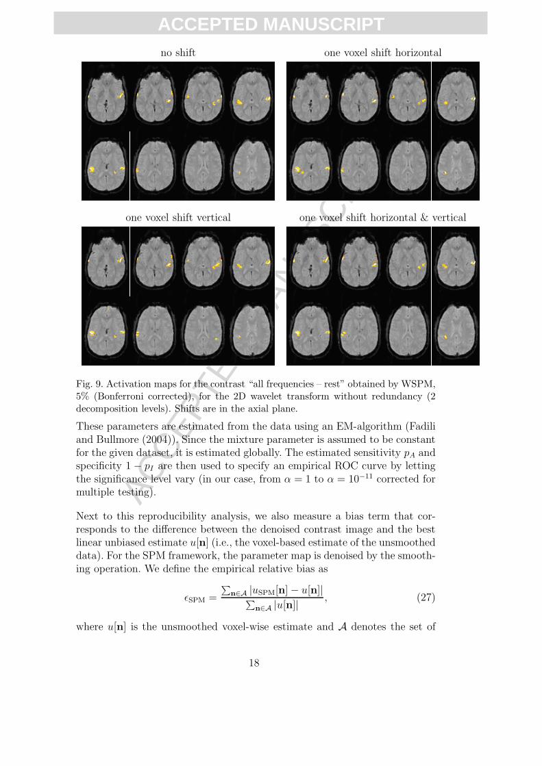
Fig. 9. Activation maps for the contrast “all frequencies – rest” obtained by WSPM,5% (Bonferroni corrected), for the 2D wavelet transform without redundancy (2decomposition levels). Shifts are in the axial plane.

These parameters are estimated from the data using an EM-algorithm (Fadiliand Bullmore (2004)). Since the mixture parameter is assumed to be constantfor the given dataset, it is estimated globally. The estimated sensitivity pA andspecificity 1 − pI are then used to specify an empirical ROC curve by lettingthe significance level vary (in our case, from α = 1 to α = 10−11 corrected formultiple testing).

Next to this reproducibility analysis, we also measure a bias term that cor-responds to the difference between the denoised contrast image and the bestlinear unbiased estimate u[n] (i.e., the voxel-based estimate of the unsmootheddata). For the SPM framework, the parameter map is denoised by the smooth-ing operation. We define the empirical relative bias as

εSPM =

∑n∈A |uSPM[n] − u[n]|∑

n∈A |u[n]| , (27)

where u[n] is the unsmoothed voxel-wise estimate and A denotes the set of

18

ACC

EPTE

D M

ANU

SCR

IPT

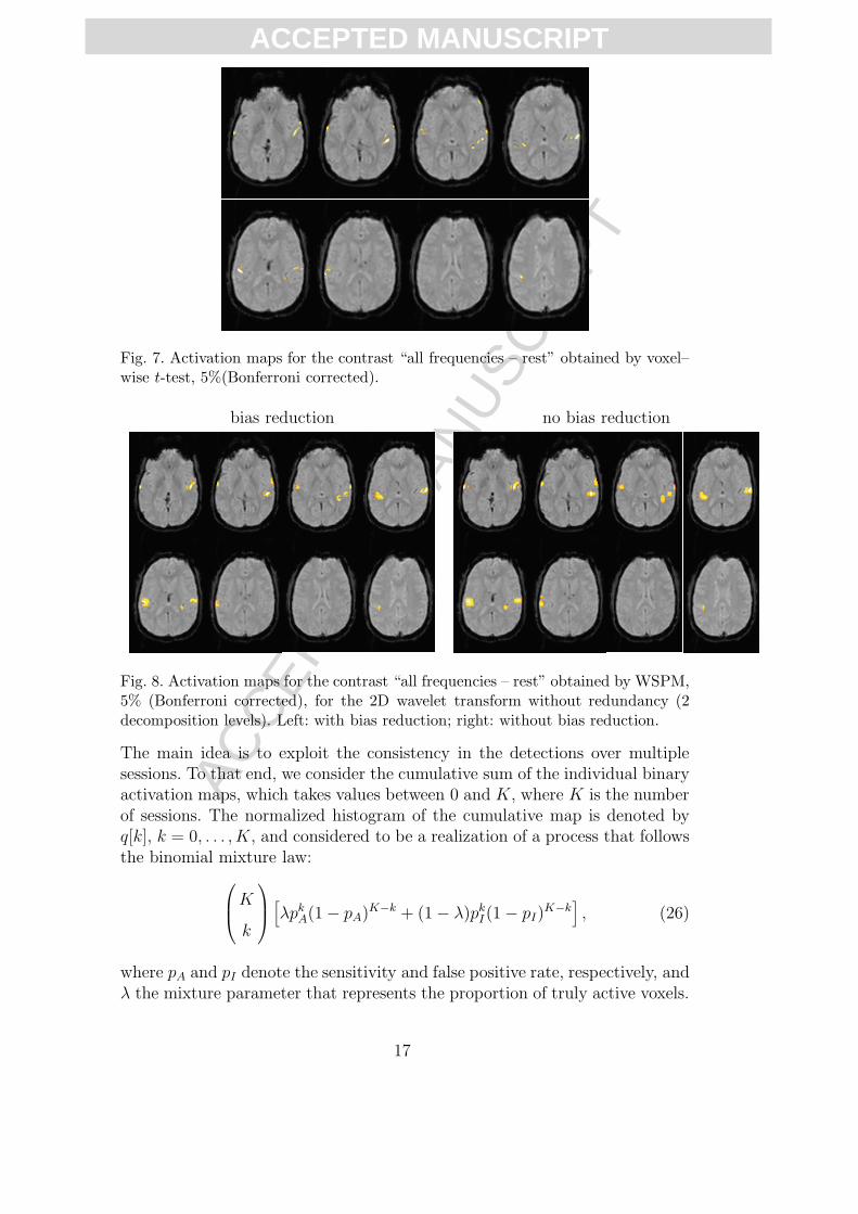
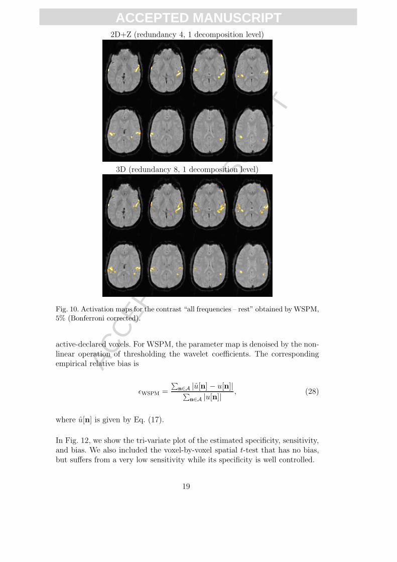
ACCEPTED MANUSCRIPT2D+Z (redundancy 4, 1 decomposition level)

3D (redundancy 8, 1 decomposition level)

Fig. 10. Activation maps for the contrast “all frequencies – rest” obtained by WSPM,5% (Bonferroni corrected).

active-declared voxels. For WSPM, the parameter map is denoised by the non-linear operation of thresholding the wavelet coefficients. The correspondingempirical relative bias is

εWSPM =

∑n∈A |u[n] − u[n]|∑

n∈A |u[n]| , (28)

where u[n] is given by Eq. (17).

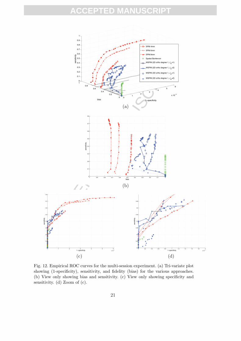
In Fig. 12, we show the tri-variate plot of the estimated specificity, sensitivity,and bias. We also included the voxel-by-voxel spatial t-test that has no bias,but suffers from a very low sensitivity while its specificity is well controlled.

19

ACC

EPTE

D M

ANU

SCR

IPT

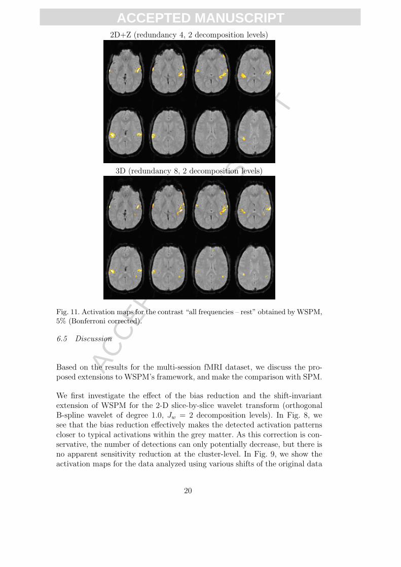
ACCEPTED MANUSCRIPT2D+Z (redundancy 4, 2 decomposition levels)

3D (redundancy 8, 2 decomposition levels)

Fig. 11. Activation maps for the contrast “all frequencies – rest” obtained by WSPM,5% (Bonferroni corrected).

6.5 Discussion

Based on the results for the multi-session fMRI dataset, we discuss the pro-posed extensions to WSPM’s framework, and make the comparison with SPM.

We first investigate the effect of the bias reduction and the shift-invariantextension of WSPM for the 2-D slice-by-slice wavelet transform (orthogonalB-spline wavelet of degree 1.0, Jw = 2 decomposition levels). In Fig. 8, wesee that the bias reduction effectively makes the detected activation patternscloser to typical activations within the grey matter. As this correction is con-servative, the number of detections can only potentially decrease, but there isno apparent sensitivity reduction at the cluster-level. In Fig. 9, we show theactivation maps for the data analyzed using various shifts of the original data

20

ACC

EPTE

D M

ANU

SCR

IPT

ACCEPTED MANUSCRIPT

01

23

45

6

x 103

0

0.2

0.4

0.6

0.8

10

0.1

0.2

0.3

0.4

0.5

0.6

0.7

0.8

0.9

1

1 specificitybias

sensitiv

ity

SPM 4mm

SPM 6mm

SPM 8mm

Spatial Bonferroni

WSPM (2D ortho degree 1, Jw

=1)

WSPM (2D ortho degree 1, Jw

=2)

WSPM (3D ortho degree 1, Jw

=1)

WSPM (3D ortho degree 1, Jw

=2)

(a)

00.10.20.30.40.50.60.70.80.910

0.1

0.2

0.3

0.4

0.5

0.6

0.7

0.8

bias

sensitiv

ity

(b)

0 1 2 3 4 5 6

x 103

0

0.1

0.2

0.3

0.4

0.5

0.6

0.7

0.8

1 specificity

sensitiv

ity

0 0.2 0.4 0.6 0.8 1 1.2 1.4 1.6 1.8 2

x 103

0.2

0.25

0.3

0.35

0.4

0.45

0.5

0.55

1 specificity

sensitiv

ity

(c) (d)

Fig. 12. Empirical ROC curves for the multi-session experiment. (a) Tri-variate plotshowing (1-specificity), sensitivity, and fidelity (bias) for the various approaches.(b) View only showing bias and sensitivity. (c) View only showing specificity andsensitivity. (d) Zoom of (c).

21

ACC

EPTE

D M

ANU

SCR

IPT

ACCEPTED MANUSCRIPTin the axial plane. The influence of such a shift is clearly not negligible andleads to different detections and shapes. Using the shift-invariant extension ofthe framework (Fig. 11, top), we see that the results for the various shifts areproperly combined. While the redundancy by a factor of 4 slightly increasesthe threshold values, there is no noticeable loss in sensitivity. From now on, weconsider only WSPM results using the bias reduction and the shift-invariantextension (4 shifts for 2-D, 8 shifts for 3-D).

We now take a closer look at the results for SPM as shown in Fig. 6. Forthis type of auditory stimulation, we expect that activated regions are mainlylocated bilaterally in the auditory cortex with more extent in the left hemi-sphere (e.g., see Bilecen et al. (1998)). Indeed, we observe different activatedfoci in the auditory cortex and extended anterior-lateral to posterior-mesialwithin the Heschl’s gyrus. Increasing the Gaussian smoothing strength resultsinto a grouping of activated clusters and an enlargement of their extent (leftauditory cortex in Fig. 6), which is in line with previous assessments of theeffects of data smoothing; e.g., Worsley et al. (1996). This increase in the spa-tial extent of activation is inherently accompanied by a decrease in the spatialdefinition (i.e. the ability to identify distinct activated foci), which might berelevant when high spatial resolution acquisitions are performed to better de-limit subdivisions of the auditory cortex or to visualize tonotopy. Critically,the activated clusters outside the auditory cortex (which are more likely tobe false positives) are also increasing with spatial smoothing, as illustrated byfrontal or occipital foci in SPM with 8mm smoothed data (Fig. 6, bottom).Finally, we notice that the sensitivity of SPM has indeed greatly improvedwith respect to the voxel-wise spatial t-test.

In Figs. 10 and 11, we show the various results for WSPM (2-D and 3-Dwavelet transform, 1 and 2 decomposition levels). In general, functional pat-terns detected by WSPM are comparable to those by SPM but with somenotable differences. Interestingly, significant clusters are localized with highspatial definition, which seems to be fairly independent of the type of wavelettransform. The 3-D transform has a higher sensitivity than the 2-D one; e.g.,a cluster located in the anterior-lateral part of the left auditory cortex is leftundetected by the 2-D transform. This superior performance can be explainedby inter-slice correlations that are exploited by the additional transform alongthe Z-direction for the 3-D transform. However, the inter-slice correlation arelocal, and having more than 1 decomposition level starts degrading the resultfor the 3-D transform. Slice timing correction did not influence the results inthis case, but it should be considered for higher TR (with non-sequential sliceacquisition schemes or event-related paradigms). For datasets with less inter-slice correlation, the use of the 2-D transform can be more appropriate sinceit is computationally faster, and its shift-invariant extension is less redundant.

The ROC curves obtained from the reproducibility study over the multiple

22

ACC

EPTE

D M

ANU

SCR

IPT

ACCEPTED MANUSCRIPTsessions are shown in Fig. 12. By definition, the voxel-wise statistical test hasno bias, but a very low sensitivity. SPM’s Gaussian smoothing introduces abias but also significantly increases sensitivity. It is interesting to see that,with WSPM, we obtain a lower bias than SPM–4mm for all types of wavelettransforms. For very high significance levels, the bias of WSPM approaches thelinear unbiased estimate. In addition to a lower bias, we also observe an im-proved ROC behavior. In particular, the 3-D transform with 1 decompositionlevel yields a higher sensitivity than SPM 4mm for the same empirical speci-ficity. The only exception is the 3-D transform with 2 decomposition levels.Finally, we note that the wiggly curves for WSPM are due to the (non-linear)thresholding operation in the wavelet domain.

These findings suggest that WSPM should be useful for high spatial resolu-tion mapping. As shown above, the false positives are well controlled, whilethe true positives are precisely localized. The latter property is a consequenceof the spatial adaptivity of the wavelet represention and of the bias reductionprocedure that tends to preserve smaller activations. Preserving localization isa key consideration in many fMRI studies. For example, investigations of theauditory cortex that try to identify cortical subdivisions or visualize tonotopyhave analyzed raw fMRI data without spatial smoothing (e.g., Talavage et al.(2000, 2004); Schonwiesner et al. (2002); Formisano et al. (2003); Seghier et al.(2005)). Indeed, it is highly desirable to preserve the high spatial resolutionprovided by the scanner and to avoid integration of signal from different vox-els that may have different functional properties. However, better resolutionusually comes at the expense of noise and many authors have employed spatialsmoothing (e.g., Bilecen et al. (2002); Wessinger et al. (2001)) to improve thesignal-to-noise ratio and to increase the sensitivity of the statistical analysis.Within this context, WSPM can be seen as an adaptive technique, in whichthe spatial filtering is performed by wavelets that can preserve edges and canpotentially recover high-resolution activation patterns. We have shown thatthis can be achieved without any compromise in sensitivity. For instance, it isnoteworthy that five different foci can be distinguished within the left auditorycortex (Fig. 10, bottom); these may correspond to subdivisions of the primaryauditory cortex (Morosan et al. (2001)) or to different secondary auditoryareas (Rivier and Clarke (1997); Talavage et al. (2000)).

In this study, we opted for the orthogonal B-spline wavelet of degree 1 (Bat-tle (1987); Unser and Blu (2000)). Thanks to orthogonality, the measurementnoise remains white in the wavelet domain; therefore, the denoising operationby coefficient-wise thresholding is very efficient. The transform has 2 vanishingmoments, which means that constant and linear trends in the data are filteredout, which could compensate for inhomogeneity effects. While the activationmaps and ROC curves for the current study show that a single decompositionlevel yields the better results, we expect a beneficial effect of more decomposi-tion levels for data with higher spatial resolution (leading to relatively larger

23

ACC

EPTE

D M

ANU

SCR

IPT

ACCEPTED MANUSCRIPTactivation patterns that can be more efficiently represented by larger basisfunctions). A similar effect has been observed when applying the frameworkto analyze data from optical imaging, as in Bathellier et al. (2007).

Finally, we recall that WSPM relies on SPM’s temporal modeling (GLM andAR-model). One shortcoming of this model is that it may produce overesti-mates when there is serial correlation in the data that has not been dealt withcorrectly. One possibility could be to deploy more advanced methods to dealwith colored noise; e.g., Bullmore et al. (2001); Fadili and Bullmore (2002).

7 Conclusions & Outlook

In this paper, we extended WSPM’s framework to further improve the re-sults for fixed-effect analysis using the spatial discrete wavelet transform. Inparticular, we proposed a simple bias reduction method, and an approach toovercome the shift-variance of the wavelet transform.

The beneficial influence of both extensions has been illustrated using syntheticand experimental data, including a comparison against SPM’s results for var-ious degrees of smoothing. This evaluation also clarified the trade-off betweenbias, sensitivity, and specificity that WSPM achieves.

We believe that the use of WSPM is particularly interesting for the analysis ofhigh spatial-resolution fMRI data, such as studies involving sensory (Beauchampet al. (2004)) or visual (Menon et al. (1997); Kim et al. (2000)) cortex. Anotherpotential area of application is clinical fMRI. Indeed, the characterisation ofperi-lesional activation is highly significant for the assessment of recovery andplasticity in patients after brain insult (e.g. Breier et al. (2004)) and it is ofparamount importance to obtain the most accurate spatial mapping.

Acknowledgments

The authors would like to thank Marco Pelizzone from the Centre romandd’implants cochleaires (University Hospital Geneva) for the experimental data.This work was supported in part by the Swiss National Science Foundationunder Grant 200020-101821 and Center for Biomedical Imaging (CIBM) ofthe Geneva - Lausanne Universities and the EPFL, as well as the foundationsLeenaards and Louis-Jeantet.

24

ACC

EPTE

D M

ANU

SCR

IPT

ACCEPTED MANUSCRIPTReferences

Aston, J., Gunn, R. N., Hinz, R., Turkheimer, F., Mar. 2005. Wavelet vari-ance components in image space for spatio-temporal neuroimaging data.NeuroImage 25 (1), 159–168.

Bathellier, B., Van De Ville, D., Blu, T., Unser, M., Carleton, A., 2007.Wavelet-based multi-resolution statistics for optical imaging signals: appli-cation to automated detection of odour activated glomeruli in the mouseolfactory bulb. NeuroImage 34, 1020–1035.

Battle, G., 1987. A block spin construction of ondelettes. Part I: Lemariefunctions. Commun. Math. Phys. 110, 601–615.

Beauchamp, M. S., Argall, B., Bodurka, J., Duyn, J., Martin, A., 2004. Un-raveling multisensory integration: patchy organization within human STSmultisensory cortex. Nature Neuroscience 7, 1190–1192.

Bilecen, D., E., S., Scheffler, K., Henning, J., Schulte, A. C., 2002. Amplitopic-ity of the human auditory cortex: an fMRI study. NeuroImage 17, 710–718.

Bilecen, D., Scheffler, K., Schmid, N., Tschopp, K., Seelig, J., 1998. Tonotopicorganization of the human auditory cortex as detected by BOLD-fMRI.Hear Res 126, 19–27.

Breier, J. I., Castillo, E. M., Boake, C., Billingsley, R., Maher, L., Francisco,G., Papanicolaou, A. C., 2004. Spatiotemporal patterns of language-specificbrain activity in patients with chronic aphasia after stroke using magne-toencephalography. NeuroImage 23, 1308–1316.

Bullmore, E., Long, C., Suckling, J., Fadili, J., Calvert, G., Zelaya, F., Car-penter, T., Brammer, M., 2001. Colored noise and computational inferencein neurophysiological time series analysis: Resampling methods in time andwavelet domains. Human Brain Mapping 12, 61–78.

Desco, M., Penedo, M., Gispert, J. D., Vaquero, J. J., Reig, S., Garcia-Barreno,P., 2005. ROC evaluation of statistical wavelet-based analysis of brain acti-vation in [15O] − H2O PET scans. NeuroImage 24, 763–770.

Fadili, M. J., Bullmore, E., 2002. Wavelet-generalised least squares: a newBLU estimator of linear regression models with 1/f errors. NeuroImage 15,217–232.

Fadili, M. J., Bullmore, E. T., 2004. A comparative evaluation of wavelet-based methods for multiple hypothesis testing of brain activation maps.NeuroImage 23 (3), 1112–1128.

Flandin, G., Penny, W. D., 2007. Bayesian fMRI data analysis with sparsespatial basis function priors. NeuroImage 34, 1108–1125.

Formisano, E., Kim, D. S., Di Salle, F., van de Moortele, P. F., Ugurbil,K., Goebel, R., 2003. Mirror-symmetric tonotopic maps in human primaryauditory cortex. Neuron 40, 859–869.

Frackowiak, R., Friston, K., Frith, C., Dolan, R., Mazziotta, J., 1997. HumanBrain Function. Academic Press.

Friston, D. J., Williams, S., Howard, R., Frackowiak, R. S., Turner, R.,1996a. Movement-related effects in fMRI time-series. Magnetic Resonance

25

ACC

EPTE

D M

ANU

SCR

IPT

ACCEPTED MANUSCRIPTin Medicine 35, 346–355.

Friston, K. J., Holmes, A., Poline, J.-B., Price, C. J., Frith, C., 1996b. Detect-ing activations in PET and fMRI: levels of inference and power. NeuroImage4, 223–235.

Friston, K. J., Holmes, A. P., Worsley, K. J., Poline, J. P., Frith, C. D., Frack-owiak, R. S. J., 1995. Statistical parametric maps in functional imaging: Ageneral linear approach. Human Brain Mapping 2, 189–210.

Friston, K. J., Josephs, O., Zarahn, E., Holmes, A. P., Poline, J.-B., 2000. Tosmooth or not to smooth? Bias and efficiency in fMRI time series analysis.NeuroImage 12, 196–208.

Friston, K. J., Penny, W., Phillips, C., Kiebel, S., Hinton, G., Ashburner, J.,2002. Classical and Bayesian inference in neuroimaging: Theory. NeuroIm-age 16, 465–483.

Genovese, C. R., Noll, D. C., Eddy, W. F., 1997. Estimating test-retest relia-bility in functional MR imaging I: Statistical methodology. Magnetic Reso-nance in Medicine 38, 497–507.

Jezzard, P., Matthews, P. M., Smith, S. M., 2001. Functional MRI an intro-duction to methods. Oxford University Press.

Johnstone, T., Ores Walsh, K. S., Greischar, L. L., Alexander, A. L., Fox,A. S., Davidson, R. J., Oakes, T. R., 2006. Motion correction and the use ofmotion covariates in multiple-subject fMRI analysis. Human Brain Mapping27, 779–788.

Kim, D. S., Duong, T. Q., Kim, S. G., 2000. High-resolution mapping of iso-orientation columns by fMRI. Nature Neuroscience 3, 164–169.

Liou, M., Su, H., Lee, J., Cheng, P., Huang, C., Tsai, C., 2003. Bridgingfunctional MR images and scientific inference: reproducibility maps. Journalof Cognitive Neuroscience 15, 935–945.

Liou, M., Su, H. R., Lee, J., Aston, J., Tsai, A., Cheng, P. E., 2006. A methodfor generating reproducible evidence in fMRI studies. NeuroImage 29, 383–395.

Maitra, R., Roys, S. R., Gullapalli, R. P., 2002. Test-retest reliability estima-tion of functional MRI data. Magnetic Resonance in Medicine 48, 62–70.

Mallat, S., 1989. A theory for multiresolution signal decomposition: Thewavelet decomposition. IEEE Trans. Pattern Anal. Mach. Intell. 11, 674–693.

Mallat, S., 1998. A Wavelet Tour of Signal Processing. Academic Press, SanDiego (CA).

Menon, R. S., Ogawa, S., Strupp, J. P., Ugurbil, K., 1997. Ocular dominancecolumns in human V1 demonstrated by functional magnetic imaging. J.Neurophysiol. 77, 2780–2787.

Morosan, P., Rademacher, J., Schleicher, A., Amunts, K., Schormann, T.,Zilles, K., 2001. Human primary auditory cortex: cytoarchitectonic subdivi-sions and mapping into a spatial reference system. NeuroImage 13, 684–701.

Mueller, K., Lohmann, G., Zysset, S., von Carmon, Y., 2003. Wavelet statisticsof functional MRI data and the general linear model. Journal of Magnetic

26

ACC

EPTE

D M

ANU

SCR

IPT

ACCEPTED MANUSCRIPTResonance Imaging 17, 20–30.

Poline, J., Worsley, K., Evans, A., Friston, K., 1997. Combining spatial extentand peak intensity to test for activations in functional imaging. NeuroImage5 (2), 83—96.

Rivier, F., Clarke, S., 1997. Cytochrome oxidase, acetylcholinesterase, andNADPPH-diapphorase staining in human supratemporal and insular cortex:evidence for multiple auditory areas. NeuroImage 6, 288–304.

Ruttimann, U., Unser, M., Rawlings, R., Rio, D., Ramsey, N., Mattay, V.,Hommer, D., Frank, J., Weinberger, D., 1998. Statistical analysis of func-tional MRI data in the wavelet domain. IEEE Transactions on MedicalImaging 17 (2), 142–154.

Schonwiesner, M., von Cramon, Y. D., Rubsamen, R., 2002. Is it tonotopyafter all? NeuroImage 17, 1144–1161.

Seghier, M. L., Boex, C., Lazeyras, F., Sigrist, A., Pelizzone, M., 2005. FMRIevidence for activation of multiple cortical regions in the primary auditorycortex of deaf subjects users of multichannel cochlear implants. CerebralCortex 15, 40–48.

Sendur, L., Maxim, V., Whitcher, B., Bullmore, E., Sep. 2005. Multiple hy-pothesis and mapping of functional MRI data in orthogonal and complexwavelet domains. IEEE Transactions on Signal Processing 53 (9), 3413–3426.

Skudlarski, P., Constable, R. T., Gore, J. C., 1999. ROC analysis of statisticalmethods used in functional MRI: individual subjects. NeuroImage 9, 311–329.

Srikanth, R., Casanova, R., Laurienti, P. J., Peiffer, A. M., Maldjian, J. A.,2006. Estimation of false discovery rate for wavelet-denoised statistical para-metric maps. NeuroImage 33, 72–84.

Talavage, T. M., Ledden, P. J., Benson, R. R., Rosen, B. R., Melcher, J. R.,2000. Frequency-dependent responses exhibited by multiple regions in hu-man auditory cortex. Hear Res 15, 225–244.

Talavage, T. M., Sereno, M., Melcher, J., Ledden, P. J., Rosen, B. R., Dale,A. M., 2004. Tonotopic organization in human auditory cortex revealed byprogressions of frequency sensitivity. J. Neurophysiol. 91, 1282–1296.

Turkheimer, F. E., Aston, J. A. D., Asselin, M.-C., Hinz, R., 2006. Multi-resolution Bayesian regression in PET dynamic studies using wavelets. Neu-roImage 32, 111–121.

Turkheimer, F. E., Brett, M., Aston, J. A. D., Leff, A. P., Sargent, P. A., Wise,R. J., Grasby, P. M., Cunningham, V. J., 2000. Statistical modelling ofpositron emission tomography images in wavelet space. Journal of CerebralBlood Flow and Metabolism 20, 1610–1618.

Unser, M., Blu, T., 2000. Fractional splines and wavelets. SIAM Review 42,43–67.

Van De Ville, D., Blu, T., Unser, M., Aug. 2003. Wavelets versus resels in thecontext of fMRI: establishing the link with SPM. In: SPIE’s Symposium onOptical Science and Technology: Wavelets X. Vol. 5207. SPIE, San Diego

27

ACC

EPTE

D M

ANU

SCR

IPT

ACCEPTED MANUSCRIPTCA, USA.

Van De Ville, D., Blu, T., Unser, M., Dec. 2004. Integrated wavelet processingand spatial statistical testing of fMRI data. NeuroImage 23 (4), 1472–1485.

Wessinger, C. M., VanMeter, J., Tian, B., Van Lare, J., Pekar, J., Rauschecker,J. P., 2001. Hierarchical organization of the human auditory cortex revealedby functional magnetic resonance imaging. J. Cogn. Neurosci. 13, 1–7.

Wink, A. M., Roerdink, J. B. T. M., Jun. 2004. Denoising functional MRimages: a comparison of wavelet denoising and Gaussian smoothing. IEEETransactions on Medical Imaging 23 (3), 374–387.

Worsley, K., Liao, C., Aston, J., Petre, V., Duncan, G., Evans, A., 2002. Ageneral statistical analysis for fMRI data. NeuroImage 15, 1–15.

Worsley, K., Marrett, S., Neelin, P., Evans, A., 1996. Searching scale space foractivation in PET images. Human Brain Mapping 4 (1), 74–90.

Worsley, K. J., Friston, K. J., 1995. Analysis of fMRI time-series revisited—again. NeuroImage 2, 173–181.

28