1

Paper SAS3258-2019

Writing a Gradient Boosting Model Node for SAS® Visual Forecasting

Yue Li, Jingrui Xie, and Iman Vasheghani Farahani, SAS Institute Inc.

ABSTRACT

SAS Visual Forecasting, the new-generation forecasting product from SAS, includes a web-based user

interface for creating and running projects that generate forecasts from historical data. It is designed to use

the highly parallel and distributed architecture of SAS® Viya®, a cloud-enabled, in-memory analytics engine

that is powered by SAS® Cloud Analytic Services (CAS), to effectively model and forecast time series on a

large scale. SAS Visual Forecasting includes several built-in modeling strategies, which serve as ready-to-

use models for generating forecasts. It also supports custom modeling nodes, where you can write and

import your own code-based modeling strategies. Similar to the ready-to-use models, these custom

modeling nodes can also be shared with other projects and forecasters. Forecasters can use SAS Visual

Forecasting to create projects by using visual flow diagrams (called pipelines), running multiple built-in or

custom models on the same data, and choosing a champion model based on the results. This paper uses

a gradient boosting model as an example to demonstrate how you can use a custom modeling node in SAS

Visual Forecasting to develop and implement your own modeling strategy.

INTRODUCTION

SAS Visual Forecasting includes a web-based user interface for creating and running projects to generate

forecasts. It provides automation and analytical sophistication to generate millions of forecasts in the fast

turnaround time that is necessary to run your business. Forecasters can create projects by using visual

flow diagrams (also called pipelines), and can run multiple models on the same data set and choose a

champion model on the basis of the forecast results.

Because SAS Visual Forecasting runs in SAS Viya, which has a highly parallel and distributed architecture,

is designed to effectively model and forecast time series on a large scale. SAS Cloud Analytic Services

(CAS) provides the speed and scalability needed to create the models and generate forecasts for millions

of time series. Massive parallel processing within a distributed architecture is one of the key advantages in

SAS Visual Forecasting for large-scale time series forecasting.

2

SAS Visual Forecasting includes a number of modeling strategies that you can use to generate forecasts.

These strategies include two hierarchical forecasting models, a panel neural network model, an auto-

forecasting model, a naïve model, a multistage forecasting model, a stacked model, and more.

Furthermore, you can create your own modeling strategies that you can share with other projects and

forecasters. These custom modeling strategies are called pluggable modeling strategies.

The following sections use a gradient boosting model (GBM) as an example to illustrate the steps for writing

a pluggable modeling strategy. Gradient boosting is a popular machine learning technique

for regression and classification problems. It produces a prediction model in the form of an ensemble of

weak prediction models. The example in this paper uses the GRADBOOST procedure in SAS® Visual Data

Mining and Machine Learning to implement a GBM. PROC GRADBOOST enables you to build a GBM that

consists of multiple decision trees.

FILES REQUIRED TO DEFINE A PLUGGABLE MODELING STRATEGY

The following files are required to define a pluggable modeling strategy in SAS Visual Forecasting 8.3:

• code.sas, which contains the SAS® code to be executed

• validation.xml, which defines the validation rules for the strategy specification settings

(properties)

• template.json, which defines the metadata of the strategy

Starting from SAS Visual Forecasting 8.4, another file is required, metadata.json. This file guarantees

that the version of the modeling strategies matches the current version of Model Studio. You can

download an existing strategy from the exchange and copy the metadata.json file to your modeling

strategy to make sure you have the correct version.

These files are packed in a .zip file for uploading to or downloading from The Exchange in SAS Visual

Forecasting. You can download an existing pluggable modeling strategy and learn from the downloaded

example files. Then you can modify the contents accordingly and use the modified files.

To download an existing pluggable modeling strategy:

3

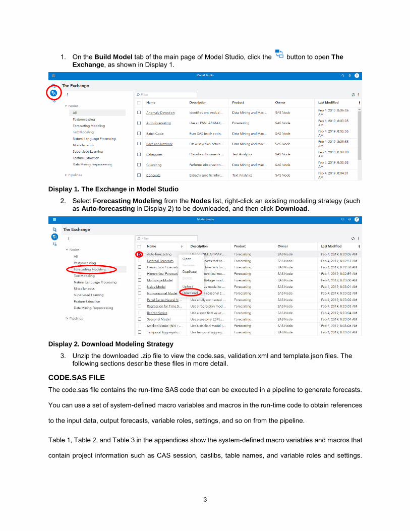
1. On the Build Model tab of the main page of Model Studio, click the button to open The Exchange, as shown in Display 1.

Display 1. The Exchange in Model Studio

2. Select Forecasting Modeling from the Nodes list, right-click an existing modeling strategy (such as Auto-forecasting in Display 2) to be downloaded, and then click Download.

Display 2. Download Modeling Strategy

3. Unzip the downloaded .zip file to view the code.sas, validation.xml and template.json files. The following sections describe these files in more detail.

CODE.SAS FILE

The code.sas file contains the run-time SAS code that can be executed in a pipeline to generate forecasts.

You can use a set of system-defined macro variables and macros in the run-time code to obtain references

to the input data, output forecasts, variable roles, settings, and so on from the pipeline.

Table 1, Table 2, and Table 3 in the appendices show the system-defined macro variables and macros that

contain project information such as CAS session, caslibs, table names, and variable roles and settings.

4

When you write the run-time code, you can refer to these macro variables and macros to retrieve information

and generate TSMODEL procedure statements.

Figure 1 shows the contents of the code.sas file, which contains the run-time code.

The code first defines a %fx_prepare_input macro that uses the built-in data preparation macro code

to prepare input data. The input table is prepared by the Data node in the pipeline. For more information

about the input data, see the chapter “Setting Up Your Project” in SAS Visual Forecasting: User’s Guide. If

you want to refer to the input table in code, you can use the macro variable definition, as follows.

&vf_libIn.."&vf_inData"n

The main code, which is wrapped in a %gbm_run macro, first calls the data preparation macro to prepare

the input and transform the dependent variable (if needed), and then calls PROC GRADBOOST to build a

gradient boosting model. When lag variables for the dependent variable are used in the model, a DATA

step is used to recursively score both the historical and future periods according to score code output from

the GBM. Another DATA step is then used to prepare the required output. At the end of the file, the main

code macro is invoked.

/*

Macro for adding features into input data

I: &vf_libIn.."&vf_inData"n

O: &vf_libOut..&vf_tableOutPrefix..&outTblName

*/

%macro fx_prepare_input(outTblName=, byVars=,

trendVariable=, seasonalDummy=,

seasonalDummyInterval=,

esmY=, lagXNumber=, lagYNumber=,

holdoutSampleSize=, holdoutSamplePercent=,

criteria=, back=);

%local filerootpath;

%let filerootpath = &sas_root_location/misc/codegenscrpt/source/sas;

%include "&filerootpath./vf_data_prep.sas";

%let temp_work_location = %sysfunc(pathname(work));

%include "&temp_work_location./vfDataPrepMacro.sas";

%mend;

/*

Main macro for forecasting using a gradient boosting model

*/

%macro gbm_run;

/*Protection against problematic _seasonDummy value*/

5

%if (not %symexist(_seasonDummy)) %then

%let _seasonDummy=&vf_timeIDInterval;

%if "&_seasonDummy" eq "" %then

%let _seasonDummy = &vf_timeIDInterval;

%if %sysfunc(INTTEST( &_seasonDummy )) eq 0 %then %do;

%put Invalid seasonal dummy interval.

Use &vf_timeIDInterval instead.;

%let _seasonDummy = &vf_timeIDInterval;

%end;

/*Parepare input data with extracted feature used for modeling*/

%fx_prepare_input(outTblName=fxInData, byVars=&vf_byVars,

trendVariable = &_trend,

seasonalDummy = &_seasonDummy,

seasonalDummyInterval = &_seasonDummyInterval,

esmY =FALSE, lagXNumber=&_lagXNumber,

lagYNumber=&_lagYNumber,

holdoutSampleSize=&_holdoutSampleSize,

holdoutSamplePercent=&_holdoutSamplePercent,

criteria=RMSE, back=0);

/*Dependent variable transformation if needed*/

%let targetVar=gbmTargetVar;

%let predictVar=P_&targetVar;

data &vf_libOut.."&vf_tableOutPrefix..fxInData"n /

SESSREF=&vf_session;

set &vf_libOut.."&vf_tableOutPrefix..fxInData"n;

&targetVar = &vf_depVar;

%if %upcase(&_depTransform) eq LOG %then %do;

if not missing(&vf_depVar) and &vf_depVar > 0 then

&targetVar = log(&vf_depVar);

else call missing(&targetVar);

%end;

run;

/*Train the gradient boosting model*/

proc gradboost data=&vf_libOut.."&vf_tableOutPrefix..fxInData"n

seed=12345;

id &vf_byVars &vf_timeID;

partition rolevar=_roleVar(TRAIN="1" VALIDATE="2" TEST="3");

input &vf_byVars /level=NOMINAL;

%if "&vf_indepVars" ne "" %then %do;

input &vf_indepVars /level=INTERVAL;

%end;

%if %intervalFeatureVarList ne %then %do;

input %intervalFeatureVarList /level=INTERVAL;

%end;

%if %nominalFeatureVarList ne %then %do;

input %nominalFeatureVarList /level=NOMINAL;

%end;

target &targetVar / level=interval;

autotune maxtime=3600

tuningparameters=( ntrees(lb=50 ub=500 init=50)) ;

%if %eval(&_lagYNumber>0) %then %do;

code file="&temp_work_location./_gbScore.sas";

%end;

%else %do;

6

output out=&vf_libOut.."scored_gb"n

copyvars=(&vf_byVars &vf_timeID &vf_depVar);

%end;

run;

%if %eval(&_lagYNumber>0) %then %do;

/*When lagYNumber is nonzero,

score the model for the whole data set with

recurrent dependent variable value for the future periods*/

%let count=%sysfunc(countw(&vf_byVars,%str( )));

%let lastByVar=%scan(&vf_byVars, &count, %str( ));

data &vf_libOut.."scored_gb"n /SINGLE=YES;

set &vf_libOut.."&vf_tableOutPrefix..fxInData"n;

by &vf_byVars &vf_timeID;

retain copyY . %do i=1 %to &_lagYNumber;

copyY_lag&i. . %end;;

gbmLastByVar = &lastByVar;

if first.gbmLastByVar then do;

copyY=.;

%do i=1 %to &_lagYNumber; copyY_lag&i.=.; %end;

end;

%do i=&_lagYNumber %to 1 %by -1;

%if &i eq 1 %then %do;

if not missing(copyY) then copyY_lag1=copyY;

%end;

%else %do;

if not missing(copyY_lag%eval(&i -1)) then

copyY_lag&i = copyY_lag%eval(&i -1);

%end;

%end;

%do i=1 %to &_lagYNumber; _lagY&i = copyY_lag&i.; %end;

%include "&temp_work_location./_gbScore.sas";

if &vf_timeID >= &vf_horizonStart then copyY = &predictVar;

else copyY = &targetVar;

drop copyY %do i=1 %to &_lagYNumber; copyY_lag&i. %end;;

run;

%end;

/*Prepare the required output tables*/

data &vf_libOut.."&vf_outFor"n;

set &vf_libOut.."scored_gb"n;

actual = &targetVar;

predict = &predictVar;

%if %upcase(&_depTransform) eq LOG %then %do;

if not missing(actual) then actual = exp(actual);

if not missing(predict) then predict = exp(predict);

%end;

%if "&vf_allowNegativeForecasts" eq "FALSE" %then %do;

if not missing(predict) and predict < 0 then predict = 0;

%end;

%if &targetVar ne &vf_depVar or &predictVar ne predict %then %do;

drop &targetVar &predictVar;

%end;

run;

%mend;

7

/*Invoke the main macro */

%gbm_run;

Figure 1. Contents of code.sas File for the Gradient Boosting Model Example

The only required output table is the OUTFOR table. The other tables are all optional.

The required OUTFOR table contains forecasts from the forecast models; it can be referred to as follows:

&vf_libOut..&vf_outFor

The OUTFOR table must have the following columns:

• byVars

• timeID

• actual (actual value of the dependent variable)

• predict (predicted value of the dependent variable)

The OUTFOR table can also have the following columns:

• std (standard deviation of errors)

• lower (lower confidence limit of predicted values)

• upper (upper confidence limit of predicted values)

SAS Visual Forecasting automatically validates the OUTFOR table and promotes it so that it can be used

as a global CAS table. If the required columns do not exist, the modeling node reports errors. SAS Visual

Forecasting also checks the OUTFOR table for invalid values (such as extreme values and negative values)

and reports warning messages if it detects any.

The optional OUTSTAT table contains forecast accuracy measures such as MAPE and RMSE; it can be

referred to as follows:

&vf_libOut..&vf_outStat

The OUTSTAT table must have the following columns:

• byVars

• summary statistics, including DFE N NOBS NMISSA NMISSP NPARMS TSS SST SSE MSE RMSE UMSE URMSE MAPE MAE RSQUARE ADJRSQ AADJRSQ RWRSQ AIC AICC SBC

8

APC MAXERR MINERR MAXPE MINPE ME MPE MDAPE GMAPE MINPPE MAXPPE MPPE MAPPE MDAPPE GMAPPE MINSPE MAXSPE MSPE SMAPE MDASPE GMASPE MINRE MAXRE MRE MRAE MDRAE GMRAE MASE MINAPES MAXAPES MAPES MDAPES GMAPES

If the pluggable modeling strategy run-time code generates this table, the pipeline will validate the table

and promote it so that it can be used as a global CAS table. If any required columns or measurements are

missing from the table or the run-time code does not output this table, the pipeline will automatically

compute the statistics and generate this table on the basis of actual and predicted series from the OUTFOR

table.

SAS Visual Forecasting automatically promotes the OUTFOR table and the OUTSTAT table (if it exists) so

that they can be used as global CAS tables. You can promote any additional output tables in the run-time

code by calling the %vf_promoteCASTable macro.

VALIDATION.XML FILE

The validation.xml file validates the specification settings against valid values in XML format. The file

conforms to an XML schema that is used to validate any XML you provide to the validation service when

you define a new validation model.

When a pluggable modeling strategy is added to a pipeline, the strategy specifications (type, name,

displayName, choicelist, and so on) are retrieved from the validation.xml file and are displayed on the right

panel of the modeling pipeline interface, with the default values defined in the template.json file and the

allowable values defined in the validation.xml file.

A validation model can be best described via an example. Display 3 shows how the GBM example modeling

node specifications are displayed in a pipeline.

9

Display 3. Modeling Pipeline Interface with the GBM Node Property

Figure 2 shows the contents of the validation.xml file for this GBM example. The root element in this file is

validationModel; it can have a name and a description as shown in Figure 2.

<?xml version="1.0" encoding="UTF-8" standalone="yes"?>

<validationModel

description="Generate forecast with Gradient Boosting Model."

name="Gradient Boosting Model" revision="0">

<links/>

<version>1</version>

<properties>

<property name="_holdoutSampleSize"

displayName="Size of data to be used for holdout"

type="integer">

<constraints>

<range min="0" includeMin="true"/>

</constraints>

</property>

<property name="_holdoutSamplePercent"

displayName="Percentage of data to be used for holdout"

type="double">

<constraints>

<range min="0" max="100"

includeMin="true" includeMax="false"/>

</constraints>

</property>

<property name="_trend"

displayName="Specifies whether to include the dependent

variable trend as an independent variable"

10

type="string">

<constraints>

<choicelist>

<choice value="None" displayValue="No trend"/>

<choice value="Linear" displayValue="Linear trend"/>

<choice value="Damptrend" displayValue="Damped trend"/>

</choicelist>

</constraints>

</property>

<property name="_seasonDummy"

displayName="Include seasonal dummy

as independent variables"

type="boolean"/>

<property name="_seasonDummyInterval"

displayName = "Time interval for creating

seasonal dummy variables"

type = "string" required="false"

enabledWhen="_seasonDummy">

</property>

<property name="_lagXNumber"

displayName="Number of lags for the independent variables"

type="integer">

<constraints>

<range min="0" includeMin="true"/>

</constraints>

</property>

<property name="_lagYNumber"

displayName="Number of lags for the dependent variable"

type="integer">

<constraints>

<range min="0" includeMin="true"/>

</constraints>

</property>

<property name="_depTransform"

displayName="Dependent variable transformation"

type="string">

<constraints>

<choicelist>

<choice value="NONE" displayValue="None"/>

<choice value="LOG" displayValue="Logistic"/>

</choicelist>

</constraints>

</property>

</properties>

</validationModel>

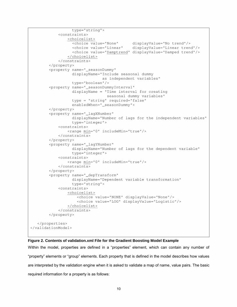
Figure 2. Contents of validation.xml File for the Gradient Boosting Model Example

Within the model, properties are defined in a “properties” element, which can contain any number of

“property” elements or “group” elements. Each property that is defined in the model describes how values

are interpreted by the validation engine when it is asked to validate a map of name, value pairs. The basic

required information for a property is as follows:

11

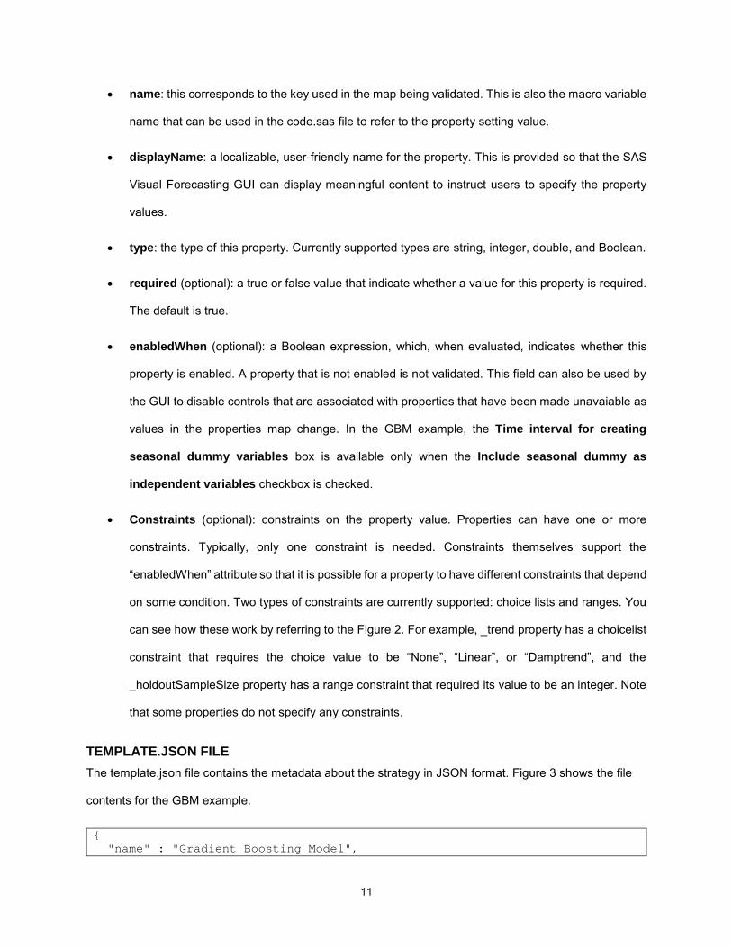
• name: this corresponds to the key used in the map being validated. This is also the macro variable

name that can be used in the code.sas file to refer to the property setting value.

• displayName: a localizable, user-friendly name for the property. This is provided so that the SAS

Visual Forecasting GUI can display meaningful content to instruct users to specify the property

values.

• type: the type of this property. Currently supported types are string, integer, double, and Boolean.

• required (optional): a true or false value that indicate whether a value for this property is required.

The default is true.

• enabledWhen (optional): a Boolean expression, which, when evaluated, indicates whether this

property is enabled. A property that is not enabled is not validated. This field can also be used by

the GUI to disable controls that are associated with properties that have been made unavaiable as

values in the properties map change. In the GBM example, the Time interval for creating

seasonal dummy variables box is available only when the Include seasonal dummy as

independent variables checkbox is checked.

• Constraints (optional): constraints on the property value. Properties can have one or more

constraints. Typically, only one constraint is needed. Constraints themselves support the

“enabledWhen” attribute so that it is possible for a property to have different constraints that depend

on some condition. Two types of constraints are currently supported: choice lists and ranges. You

can see how these work by referring to the Figure 2. For example, _trend property has a choicelist

constraint that requires the choice value to be “None”, “Linear”, or “Damptrend”, and the

_holdoutSampleSize property has a range constraint that required its value to be an integer. Note

that some properties do not specify any constraints.

TEMPLATE.JSON FILE

The template.json file contains the metadata about the strategy in JSON format. Figure 3 shows the file

contents for the GBM example.

{

"name" : "Gradient Boosting Model",

12

"description" : "Generate forecast with Gradient Boosting Model.",

"revision" : 0,

"version" : 1,

"prototype" : {

"name" : "Gradient Boosting Model",

"revision" : 0,

"executionProviderId" : "Compute",

"status" : "undefined",

"componentProperties" : {

"_holdoutSampleSize": 0,

"_holdoutSamplePercent": 20,

"_trend": "Linear",

"_seasonDummy": true,

"_lagXNumber": 0,

"_lagYNumber": 0,

"_depTransform": "NONE",

"preProcessTransformationsCode": ""

}

},

"applicationId" : "forecasting",

"classification" : "pluggable",

"providerId" : "CustomTemplate",

"group" : "modeling",

"hidden" : false

}

Figure 3. Contents of template.json File for the Gradient Boosting Model Example

The following information is included in this file:

• name: name of the strategy; this name will be displayed as the name of the node

• description: description of the strategy; this description will be displayed as the description of the

node

• revision: revision information

• version: version information

• prototype

o name: Specify the same value as the first name field

o revision: Specify the same value as the first revision field

o executionProviderId: Specify “Compute”

o status: Specify “undefined”

13

o componentProperties: contains the specifications and the corresponding default values.

The file can contain two types of properties:

▪ Model properties: In this example, seven out of the eight specifications that are

defined in the validation.xml file are declared in this file with default values. It is not

necessary to declare the "_seasonDummyInterval” option because

required="false" is specified in the validation.xml file.

▪ Process property: You also need to include one additional property called

preProcessTransformationsCode with default value set to “” to make sure the

pipeline works as expected.

• applicationId: Specify the application, which can be “forecasting”, “text”, or “datamining”. The value

“forecasting” should always be used for SAS Visual Forecasting strategies.

• classification: Specify “pluggable”

• providerId: Specify “CustomTemplate”

• group: Specify “modeling”

• hidden: Specify false

PUTTING EVERYTHING TOGETHER

After you create a .zip file from the files of the pluggable modeling strategy, you can upload the .zip file

through The Exchange as follows:

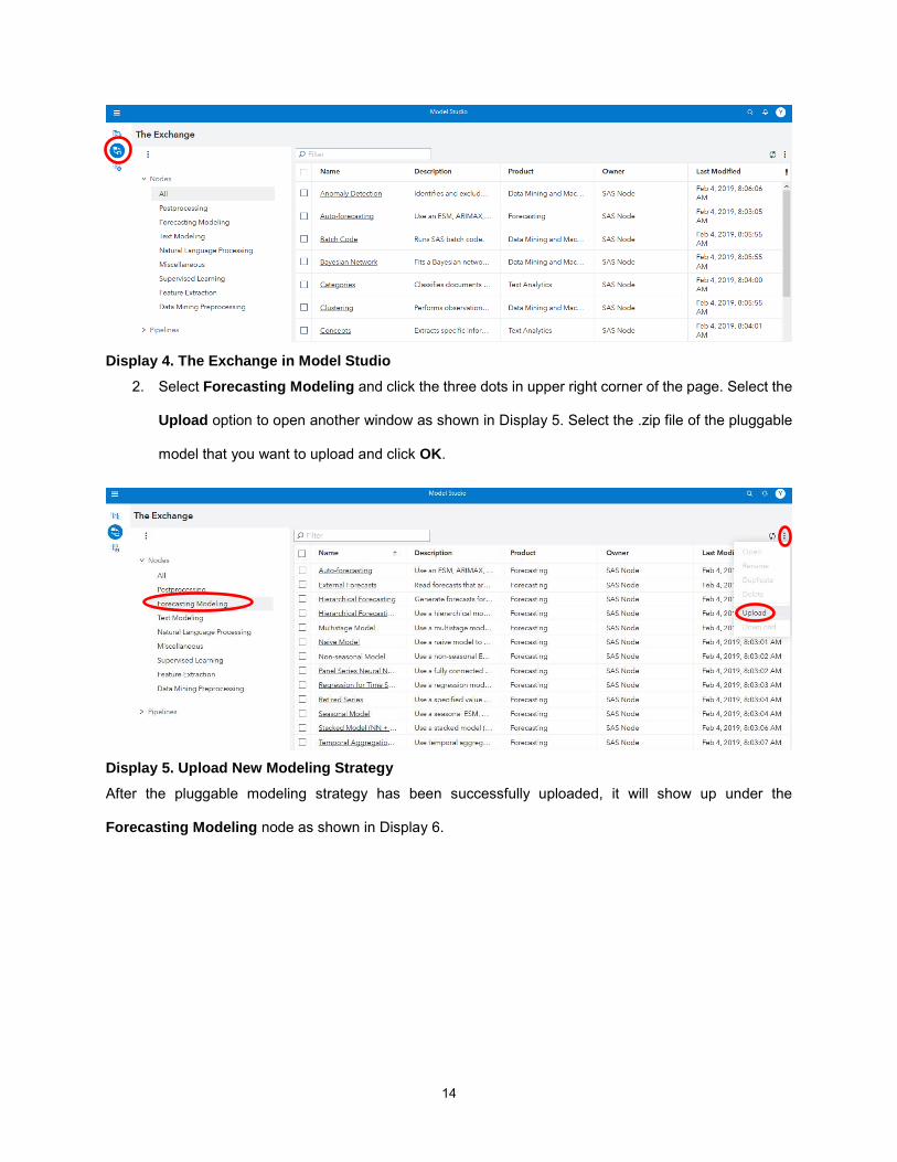
1. On the Build Model tab of the main page of Model Studio, click the button to open The

Exchange.

14

Display 4. The Exchange in Model Studio

2. Select Forecasting Modeling and click the three dots in upper right corner of the page. Select the

Upload option to open another window as shown in Display 5. Select the .zip file of the pluggable

model that you want to upload and click OK.

Display 5. Upload New Modeling Strategy

After the pluggable modeling strategy has been successfully uploaded, it will show up under the

Forecasting Modeling node as shown in Display 6.

15

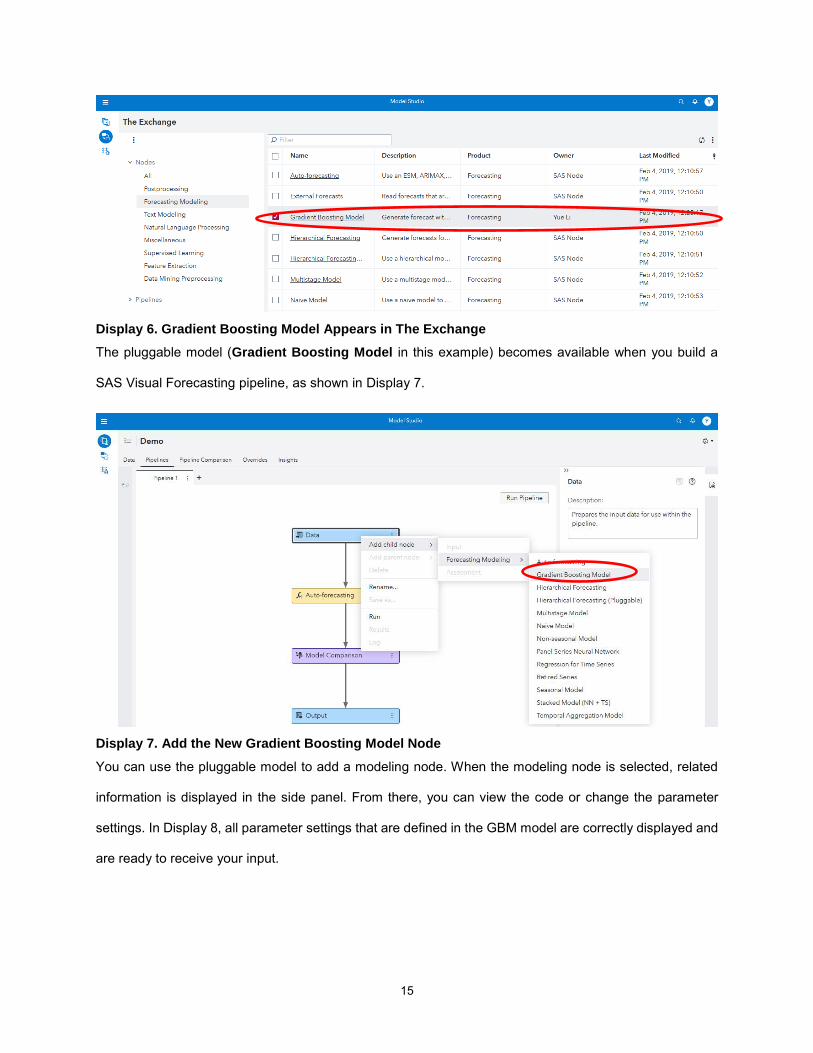
Display 6. Gradient Boosting Model Appears in The Exchange

The pluggable model (Gradient Boosting Model in this example) becomes available when you build a

SAS Visual Forecasting pipeline, as shown in Display 7.

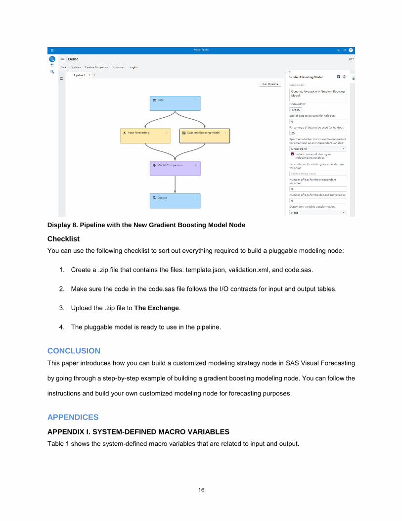
Display 7. Add the New Gradient Boosting Model Node

You can use the pluggable model to add a modeling node. When the modeling node is selected, related

information is displayed in the side panel. From there, you can view the code or change the parameter

settings. In Display 8, all parameter settings that are defined in the GBM model are correctly displayed and

are ready to receive your input.

16

Display 8. Pipeline with the New Gradient Boosting Model Node

Checklist

You can use the following checklist to sort out everything required to build a pluggable modeling node:

1. Create a .zip file that contains the files: template.json, validation.xml, and code.sas.

2. Make sure the code in the code.sas file follows the I/O contracts for input and output tables.

3. Upload the .zip file to The Exchange.

4. The pluggable model is ready to use in the pipeline.

CONCLUSION

This paper introduces how you can build a customized modeling strategy node in SAS Visual Forecasting

by going through a step-by-step example of building a gradient boosting modeling node. You can follow the

instructions and build your own customized modeling node for forecasting purposes.

APPENDICES

APPENDIX I. SYSTEM-DEFINED MACRO VARIABLES

Table 1 shows the system-defined macro variables that are related to input and output.

17

Macro Variable Description

vf_session CAS session name vf_sessionID CAS session ID vf_caslibIn caslib where input data is stored vf_caslibOut caslib where output data is stored vf_libIn CAS engine libref for input data vf_libOut CAS engine libref for output data vf_tableInPrefix Input table name prefix, which is used to differentiate input tables among different

projects vf_tableOutPrefix Output table name prefix, which is used to differentiate output tables among

different projects vf_inData Input table name Vf_inAttribute Input attribute table name vf_outFor Output forecast table name vf_outStat Output statistics table name vf_outInformation Output information table name vf_outSelect Output model selection table name vf_outModelInfo Output model information table name vf_outLog Output log name

Table 1. System-Defined Macro Variables That Are Related to Input and Output

Table 2 shows the macro variables that are related to data specification.

Macro Variable Description

vf_depVar Dependent variable name vf_depVarAcc Accumulation setting for the dependent variable vf_depVarAgg Aggregation setting for the dependent variable vf_depVarSetMissing Missing-value interpretation setting for the dependent variable vf_byVars BY variables defined for the project vf_timeID Time ID variable name vf_timeIDInterval Time series interval vf_timeIDSeasonality Time series seasonality vf_setMissing Missing-value interpretation setting for the time ID vf_lead Forecast lead vf_horizonStart Forecast horizon start date vf_reconcileLevelNumber Reconcile level number specified for the project; the _TOP_ level

number is 0 vf_reconcileLevel BY variable that corresponds to the reconcile level specified for the

project vf_allowNegativeForecasts Boolean value indicating whether negative values are allowed in the

forecast results vf_indepVars Strings that specify the independent variable names (for example,

promotion, price, and inventory) vf_indepVarsAcc Accumulation settings for the independent variables vf_indepVarsAgg Aggregation settings for the independent variables vf_indepVarsSetMissing Missing-value interpretation settings for the independent variables

18

Macro Variable Description

vf_indepVarsRequired Specification of whether independent variables are required (YES, NO) vf_indepVarsExtend Forecast method for extension vf_events List of events defined in the project vf_eventsRequired Specification of whether the events are required vf_inEventData Event definition data vf_inEventObj inEventObj with all event data definitions specified, which can be used in

PROC TSMODEL with the ATSM package

Table 2. Macro Variables That Are Related to Data Specification

APPENDIX II. SYSTEM-DEFINED MACROS

Table 3 shows the system-defined macros.

Macro Description

%vf_depVarTSMODEL Declares the dependent variable for PROC TSMODEL (Note 1)

%vf_indepVarsTSMODEL Declares the independent variables for PROC TSMODEL (Note 1)

%vf_varsTSMODEL Declares statement both the dependent variable and independent variables for PROC TSMODEL (Note 1)

%vf_addXTSMODEL(tsdf) Adds independent variables tothe ATSM package data frame in PROC TSMODEL (Note 2)

%vf_addEvents(tsdf, eventsObj) Declares and adds event specification to the ATSM package data frame and event object in PROC TSMODEL (Note 3)

%vf_promoteCASTable(localCASTable = , globalCASTable = )

Promotes a local CAS table to a global CAS table (Note 4)

Table 3. List of Macros

Notes:

1. The %vf_varsTSMODEL macro generates the VAR statements of the PROC TSMODEL to define

the dependent and independent variables. It combines the statements that are generated by the

%vf_depVarTSMODEL and %vf_indepVarsTSMODEL macros. The statements also include the

ACC= and SETMISS= settings for the corresponding variables. For example, when there is one

dependent variable, y, and two independent variables, x1 and x2, the macro generates the following

statement:

var y /acc=SUM setmiss=MISSING;

var x1/acc=AVG setmiss=AVG;

var x2/acc=AVG setmiss=FIRST;

2. The %vf_addXTSMODEL macro generates an addX function call of the Time Series Data Frame

(TSDF) object from the Automatic Time Series Modeling (ATSM) package for all the independent

variables. The following example shows the use of the %vf_addXTSMODEL macro:

19

declare object dataFrame(tsdf);

%if "&vf_indepVars" ne "" %then %do;

%vf_addXTSMODEL(dataFrame);

%end;

3. The %vf_addEvents macro adds event specifications of the TSDF object and the event object from

the ATSM package. The following example shows the use of the %vf_addEvents macro:

declare object dataFrame(tsdf);

%if "&vf_inEventObj" ne "" or "&vf_events" ne "" %then %do;

declare object ev1(event);

rc = ev1.Initialize();

%vf_addEvents(dataframe, ev1);

%end;

4. The %vf_promoteCASTable macro promotes a local CAS table to the global level. If you want to

make any table other than the system-defined output tables available for further use, you need to

use the %vf_promoteCASTable macro to promote them.

CONTACT INFORMATION

Your comments and questions are valued and encouraged. Contact the author:

Iman Vasheghani FarahaniSAS Institute Inc Iman.VasheghaniFarahani@sas.com

SAS and all other SAS Institute Inc. product or service names are registered trademarks or trademarks of SAS Institute Inc. in the USA and other countries. ® indicates USA registration.

Other brand and product names are trademarks of their respective companies.