WP5.2: Combination of MAR and adjusted conventional ...

© 2011 TECHNEAU TECHNEAU is an Integrated Project Funded by the European Commission under the Sixth Framework Programme, Sustainable Development, Global Change and Ecosystems Thematic Priority Area (contractnumber 018320). All rights reserved. No part of this book may be reproduced, stored in a database or retrieval system, or published, in any form or in any way, electronically, mechanically, by print, photoprint, microfilm or any other means without prior written permission from the publisher

WP5.2: Combination of MAR and adjusted conventional treatment processes for an Integrated Water Resources Management

Deliverable 5.2.10 Comparative cost analysis for BF systems and direct surface water use under different boundary conditions

Techneau, March 2011

© TECHNEAU Executive Summary

Summary Work package WP 5.2 “Combination of Managed Aquifer Recharge (MAR) and adjusted conventional treatment processes for an Integrated Water Resources Management“ within the European Project TECHNEAU (“Technology enabled universal access to safe water”) investigates bank filtration (BF) + post-treatment as a MAR technique to provide sustainable and safe drinking water supply to developing and newly industrialised countries. One of the tasks within this work package is to assess the cost-efficiency of BF systems. For this a comparative cost analysis (CCA) between groundwater waterworks using BF as natural pre-treatment step and surface water treatment plants (SWTPs) is performed. The CCA yielded that, under the assumption of equally low surface water quality, BF systems are more cost-efficient than SWTPs. This result is in line with the general water source priority of water suppliers, which prefer resources with the best water quality and security under the constraint of guaranteeing sufficient water availability. Furthermore the sensitivity analysis confirmed that the natural boundary condition 'pumping rate per production well' has a major impact on the specific total costs of BF systems. Lower pumping rates lead to increasing capital costs for the additional production wells, which are not fully compensated through pumping cost savings and thus lead to increasing total costs. In addition the result of the monitoring scenario clearly confirmed that for this aspect groundwater waterworks have a structural disadvantage compared to surface waterworks. Subsequently, if monitoring costs are taken into account, a higher critical pumping rate per production well is required to exceed the break-even-point. In a nutshell the CCA shall support water supply managers in the complex process of making rational investment decisions. However, since within this analysis only water abstraction and treatment process costs are considered, the CCA does not cover the total cost structure of a waterworks (e.g. costs of building sites). Thus the application of the CCA is only valid if both (i) neglected costs and (ii) benefits are in the same order of magnitude for all alternatives (exception: most cost-efficient alternative provides excess benefits). In case that the above stated prerequisites are not fulfilled, the CCA is only a first step in the economic assessment and more powerful evaluation methods (e.g. cost-benefit analysis) are needed. Contact Michael Rustler, Dipl.-Geoök., KompetenzZentrum Wasser Berlin gGmbH Email: [email protected] Phone: +49 (0) 30 536 53 825 Dr. Gesche Grützmacher, KompetenzZentrum Wasser Berlin gGmbH Email: [email protected] Phone: +49 (0) 30 536 53 813

Comparative cost analysis for BF systems and direct surface water use under different boundary conditions

March, 2011


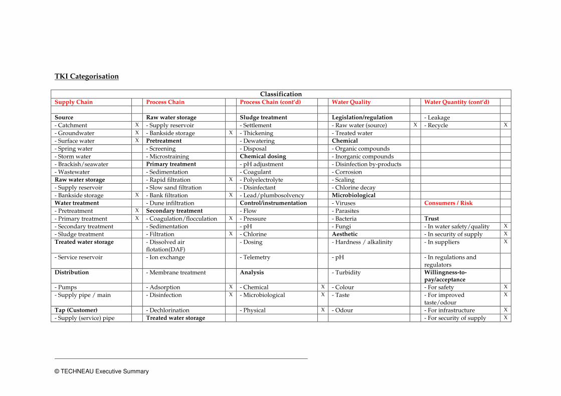
TKI Categorisation

Classification Supply Chain Process Chain Process Chain (cont’d) Water Quality Water Quantity (cont’d)

Source Raw water storage Sludge treatment Legislation/regulation - Leakage

- Catchment X - Supply reservoir - Settlement - Raw water (source) X - Recycle X

- Groundwater X - Bankside storage X - Thickening - Treated water

- Surface water X Pretreatment - Dewatering Chemical

- Spring water - Screening - Disposal - Organic compounds

- Storm water - Microstraining Chemical dosing - Inorganic compounds

- Brackish/seawater Primary treatment - pH adjustment - Disinfection by-products

- Wastewater - Sedimentation - Coagulant - Corrosion

Raw water storage - Rapid filtration X - Polyelectrolyte - Scaling

- Supply reservoir - Slow sand filtration - Disinfectant - Chlorine decay

- Bankside storage X - Bank filtration X - Lead/plumbosolvency Microbiological

Water treatment - Dune infiltration Control/instrumentation - Viruses Consumers / Risk

- Pretreatment X Secondary treatment - Flow - Parasites

- Primary treatment X - Coagulation/flocculation X - Pressure - Bacteria Trust

- Secondary treatment - Sedimentation - pH - Fungi - In water safety/quality X

- Sludge treatment - Filtration X - Chlorine Aesthetic - In security of supply X

Treated water storage - Dissolved air flotation(DAF)

- Dosing - Hardness / alkalinity - In suppliers X

- Service reservoir - Ion exchange - Telemetry - pH - In regulations and regulators

Distribution - Membrane treatment Analysis - Turbidity Willingness-to-pay/acceptance

- Pumps - Adsorption X - Chemical X - Colour - For safety X

- Supply pipe / main - Disinfection X - Microbiological X - Taste - For improved taste/odour

X

Tap (Customer) - Dechlorination - Physical X - Odour - For infrastructure X

- Supply (service) pipe Treated water storage - For security of supply X


Internal plumbing - Service reservoir Water Quantity Risk Communication

- Internal storage Distribution - Communication strategies

- Disinfection Source - Potential pitfalls

- Lead/plumbosolvency - Source management X - Proven techniques X

- Manganese control - Alternative source(s) X

- Biofilm control Management

Tap (Customer) - Water balance X

- Point-of-entry (POE) - Demand/supply trend(s) X

- Point-of-use (POU) - Demand reduction

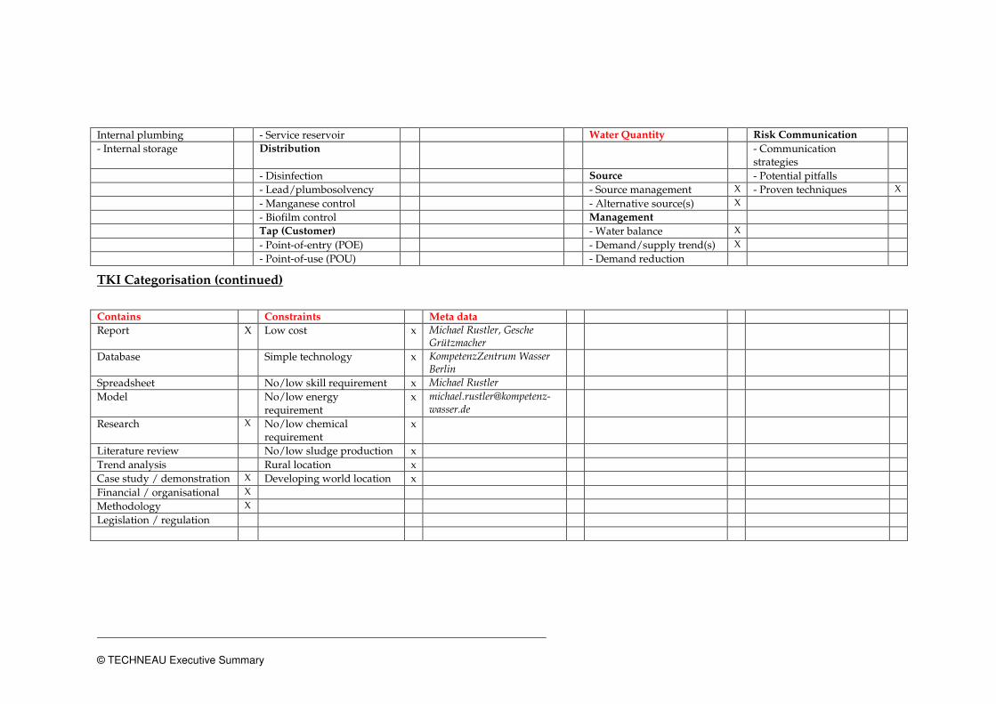
TKI Categorisation (continued)

Contains Constraints Meta data

Report X Low cost x Michael Rustler, Gesche Grützmacher

Database Simple technology x KompetenzZentrum Wasser Berlin

Spreadsheet No/low skill requirement x Michael Rustler Model No/low energy

requirement x michael.rustler@kompetenz-

wasser.de

Research X No/low chemical requirement

x

Literature review No/low sludge production x Trend analysis Rural location x Case study / demonstration X Developing world location x Financial / organisational X Methodology X Legislation / regulation

Colophon

Title Comparative cost analysis for BF systems and direct surface water use under different boundary conditions Authors Michael Rustler (KWB), Ulf Miehe (KWB), Gesche Grützmacher (KWB) Quality Assurance By Christian Remy (KWB), Gegina Gnirss (BWB), Glenn Dillon (WRc) Deliverable number D 5.2.10

This report is: PU (for public)

TECHNEAU report 5.2.10

© TECHNEAU - i - 07 March 2011

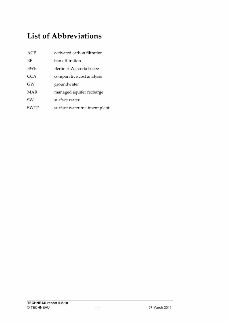
List of Abbreviations

ACF activated carbon filtration

BF bank filtration

BWB Berliner Wasserbetriebe

CCA comparative cost analysis

GW groundwater

MAR managed aquifer recharge

SW surface water

SWTP surface water treatment plant


© TECHNEAU - ii - 07 March 2011

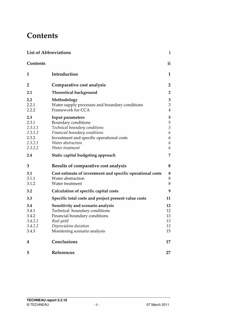
Contents

List of Abbreviations i

Contents ii

1 Introduction 1

2 Comparative cost analysis 2

2.1 Theoretical background 2

2.2 Methodology 3

2.2.1 Water supply processes and boundary conditions 3

2.2.2 Framework for CCA 4

2.3 Input parameters 5

2.3.1 Boundary conditions 5

2.3.1.1 Technical boundary conditions 5

2.3.1.2 Financial boundary conditions 6

2.3.2 Investment and specific operational costs 6

2.3.2.1 Water abstraction 6

2.3.2.2 Water treatment 6

2.4 Static capital budgeting approach 7

3 Results of comparative cost analysis 8

3.1 Cost estimate of investment and specific operational costs 8

3.1.1 Water abstraction 8

3.1.2 Water treatment 8

3.2 Calculation of specific capital costs 9

3.3 Specific total costs and project present value costs 11

3.4 Sensitivity and scenario analysis 12

3.4.1 Technical boundary conditions 12

3.4.2 Financial boundary conditions 13

3.4.2.1 Real yield 13

3.4.2.2 Depreciation duration 13

3.4.3 Monitoring scenario analysis 15

4 Conclusions 17

5 References 27


© TECHNEAU - 1 - 07 March 2011

1 Introduction

Context

Work package WP5.2 “Combination of Managed Aquifer Recharge (MAR) and adjusted conventional treatment processes for an Integrated Water Resources Management“ within the European Project TECHNEAU (“Technology enabled universal access to safe water”) investigates bank filtration (BF) + post-treatment as a MAR technique to provide sustainable and safe drinking water to developing and newly-industrialised countries. One of the tasks within this work package is to assess the cost-efficiency of BF systems. This report summarizes the outcomes of this analysis and shall support water supply managers in the complex process of making rational investment decisions. Background and Aim

On the one hand BF as a natural pre-treatment step has a structural advantage for the water treatment process compared to direct surface water use, since it is a low-tech and low-cost technology (e.g. SHAMRUKH & ABDEL-WAHAB 2008). On the other hand this initial benefit could be offset through excess expenditures for the water abstraction process, due to higher operational and capital costs if raw water is extracted from wells. However, to the authors’ knowledge there is no publication that quantitatively evaluates the cost-efficiency of BF systems by taking operational and capital costs for both water supply processes into account (e.g. CHAWEZA 2006 reports only operational costs). Thus it is the aim of this report to assess whether groundwater waterworks using BF as natural pre-treatment step really have a cost advantage compared to direct surface water use if both, water abstraction and treatment processes are considered. In addition the impact of (i) site-specific boundary conditions (e.g. technical, financial) and (ii) different monitoring demand of groundwater and surface water abstractions on the cost-efficiency of BF systems is assessed in the framework of a sensitivity and scenario analysis.



2 Comparative cost analysis

2.1 Theoretical background

The information on the comparative cost analysis (CCA) is completely compiled from (LAWA 2005) and the interested reader is referred to this publication for further methodological details. The objective of the CCA is to select the most cost-efficient solution out of different alternatives that satisfies a predefined performance criterion (here: produced water in compliance with drinking water ordinance, i.e. TRINKWV 2001 in Germany). According to LAWA (2005) the application of the CCA is limited to the following prerequisites:

- normative objective (predefined performance is stringent to provide) - benefit equity of alternatives, exception: the more cost-efficient alternative shows in

addition the most benefit excess compared to the other alternatives - equivalence of monetary non-assessable cost effects, e.g. in monetary terms non-

assessable negative consequences (intangible social costs) must not be important or have to be in the same order of magnitude for all considered alternatives, since they are not considered in the CCA.

As a consequence the comparative cost analysis is only useful if (i) a relative economic comparison is sufficient and (ii) the considered alternatives are equivalent concerning their benefits and social costs. This prerequisite is not fulfilled if surface water and groundwater (bank filtration) abstraction alternatives are evaluated, since BF has additional benefits compared to surface water (e.g. temporal mitigation of abstraction impacts on surface water body, improved source water reliability). However, this limitation does not matter as long as the total costs of the BF alternative do not exceed the costs of the surface water alternative. If this prerequisite is not fulfilled the CCA is only the first step in the overall assessment and more powerful evaluation methods (e.g. cost-benefit analysis) are needed in order to cover the required information need for making a rational investment decision (see Appendix A, Table 4 for a systematic comparison of available economic evaluation methods). Note that the objective of the CCA is limited to find the most cost-efficient investment alternative and cannot be used for financial budgeting, asset valuation or bill of charges. For these purposes a separate assessment is needed to avoid fundamental errors. Consequently the CCA supports water supply managers in the complex planning process of future investment decisions.



2.2 Methodology

2.2.1 Water supply processes and boundary conditions

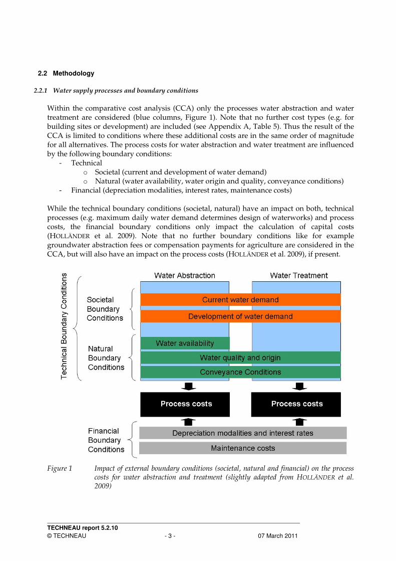
Within the comparative cost analysis (CCA) only the processes water abstraction and water treatment are considered (blue columns, Figure 1). Note that no further cost types (e.g. for building sites or development) are included (see Appendix A, Table 5). Thus the result of the CCA is limited to conditions where these additional costs are in the same order of magnitude for all alternatives. The process costs for water abstraction and water treatment are influenced by the following boundary conditions:

- Technical o Societal (current and development of water demand) o Natural (water availability, water origin and quality, conveyance conditions)

- Financial (depreciation modalities, interest rates, maintenance costs) While the technical boundary conditions (societal, natural) have an impact on both, technical processes (e.g. maximum daily water demand determines design of waterworks) and process costs, the financial boundary conditions only impact the calculation of capital costs (HOLLÄNDER et al. 2009). Note that no further boundary conditions like for example groundwater abstraction fees or compensation payments for agriculture are considered in the CCA, but will also have an impact on the process costs (HOLLÄNDER et al. 2009), if present.

Figure 1 Impact of external boundary conditions (societal, natural and financial) on the process

costs for water abstraction and treatment (slightly adapted from HOLLÄNDER et al. 2009)



2.2.2 Framework for CCA

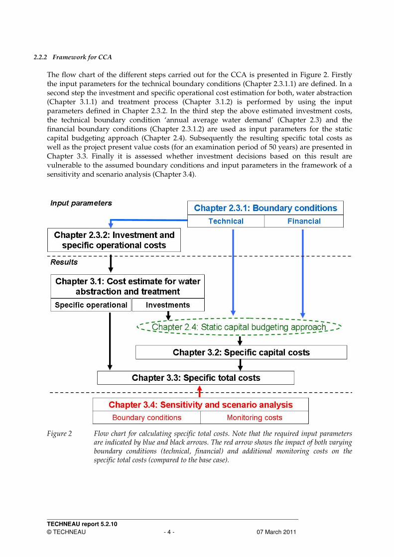
The flow chart of the different steps carried out for the CCA is presented in Figure 2. Firstly the input parameters for the technical boundary conditions (Chapter 2.3.1.1) are defined. In a second step the investment and specific operational cost estimation for both, water abstraction (Chapter 3.1.1) and treatment process (Chapter 3.1.2) is performed by using the input parameters defined in Chapter 2.3.2. In the third step the above estimated investment costs, the technical boundary condition ‘annual average water demand’ (Chapter 2.3) and the financial boundary conditions (Chapter 2.3.1.2) are used as input parameters for the static capital budgeting approach (Chapter 2.4). Subsequently the resulting specific total costs as well as the project present value costs (for an examination period of 50 years) are presented in Chapter 3.3. Finally it is assessed whether investment decisions based on this result are vulnerable to the assumed boundary conditions and input parameters in the framework of a sensitivity and scenario analysis (Chapter 3.4).

Figure 2 Flow chart for calculating specific total costs. Note that the required input parameters

are indicated by blue and black arrows. The red arrow shows the impact of both varying boundary conditions (technical, financial) and additional monitoring costs on the specific total costs (compared to the base case).



2.3 Input parameters

2.3.1 Boundary conditions

2.3.1.1 Technical boundary conditions The following input parameters and scenarios are used to represent the technical boundary conditions (see Figure 1) in the CCA:

- Water demand: it is assumed that the annual average water demand is 10.000.000 m³/a (drinking water supply from maximum 238.237 inhabitants assuming a per capita demand of 115 l/d) and the maximum daily water demand is 46.565 m³/d (peak load factor: 1.7, MÖLLER & BURGSCHWEIGER 2008). Consequently the waterworks treatment plant is designed for a maximum capacity of 46.565 m³/d, which is equal to the maximum daily water demand (assumption of a water storage tank to balance shorter water demand fluctuations). In addition a 10% capacity redundancy is assumed for water abstraction due to possible maintenance interruptions (maximum abstraction capacity: 49.315 m³/d). Note that the annual average water demand is only relevant for the static capital budgeting approach (see Chapter 2.4).

- Water availability: it is assumed that groundwater and surface water availability are sufficient, so that no additional raw water has to be imported from other water suppliers. However, in case of groundwater abstractions the maximum pumping rate per production well is limited by the hydrogeological setting. For the CCA a value of 100 m³/h is assumed, which is in line with BWB data (median value: 89 m³/h, ORLIKOWSKI & SCHWARZMÜLLER 2009)

- Water quality and origin: in Table 1 scenarios are defined which represent (i) three waterworks with comparable low surface water qualities but different raw water qualities and (ii) one waterworks with very good surface and raw water quality. The latter is not directly comparable with the other ones but can serve as a reference scenario to assess their structural disadvantage! Note that the four scenarios are based on the treatment process schemes of real waterworks but do not take further costs into account (e.g. costs for building sites or development).

- Conveyance conditions: it is assumed that the lifting height for groundwater abstractions is 14 m (average hydraulic head of production wells below ground level based on BWB data: 11m + estimated additional lifting height to waterworks: 3m) while only 3 m is required for surface water abstractions (see also Chapter 2.3.2.1).

Table 1 Natural boundary condition: surface and raw water quality scenarios (SW: surface water, GW: groundwater); Note that the four raw water quality scenarios require distinct water treatment schemes for drinking water production, which are presented in detail in Appendix A Table 7

Scenario Type 'Lake Constance'

Type 'Rostock-Warnow'

Type 'Mühlheim' Type 'Berlin'

Water Source SW SW GW (short BF, <10d) GW (long BF, >50d)

Surface Water Quality Low

Raw Water Quality Very good

Low Medium (DOC: -20%) Good (DOC: -20%, no microorganisms but

Fe/Mn)



2.3.1.2 Financial boundary conditions For the financial boundary conditions (see Figure 1) the following input parameters are defined which are required for the static capital budgeting approach (see Chapter 2.4):

- Interest rate: real yield of 3% (recommendation according to LAWA 2005) for average fixed capital (50% of investment costs) is used instead of nominal interest rate (e.g. BWB: 6.5%). This assumes an inflation rate of 3.5%.

- Depreciation duration [a]: equal with average lifetime of infrastructure o 50 years: buildings, wells o 25 years: raw water pipe o 12.5 years: equipment, filters

- Maintenance factor [%] o 0.5% of investment costs p.a. for buildings o 2% of investment costs p.a. for wells, equipment, filters and raw water pipe

2.3.2 Investment and specific operational costs

2.3.2.1 Water abstraction The investment costs include the construction of the water abstraction sytems. For groundwater abstraction it is assumed that the pumping rate per production well is limited to 100m³/h. As a consequence 23 production wells (including a 10% redundancy for maintenance reasons) are needed to deliver the required raw water. It is further assumed that the investment costs per production well are 121.000 € (MUTSCHMANN & STIMMELMAYR 2007) which is in line with actual costs of the water supplier BWB. In case of surface water abstraction it is assumed that the infrastructure costs only account 30% of the construction costs for the production wells (conservative ‘worst-case’ estimate). Furthermore it is assumed that for BF additional 5000m raw water pipes are needed with 300€ costs per running meter (KRINGS & DÜLLMANN 2002). For the specific operational water abstraction costs only pumping costs are considered (see Appendix A, Table 6) and the following assumptions are used for the calculation:

• Lifting height of 14 m for BF and 3m for surface water (estimated) • Electrical energy demand: 0.2 kWh/m³ (BWB data) • Electricity tariff: 0.13 €/kWh (estimated) • Scaling of BF pumping costs per meter lifting height (assumption: no further head

losses in raw water pipe)

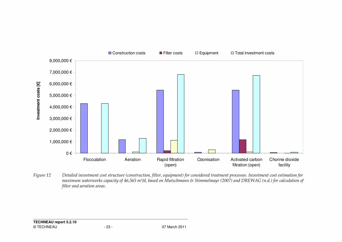
2.3.2.2 Water treatment The investment costs for water treatment processes are estimated from MUTSCHMANN & STIMMELMAYR (2007) on process scale (see Appendix A, Table 7 and Figure 12). In addition the calculation of the required filter and aeration areas is based on the real treatment process design of the waterworks Dresden-Hosterwitz (DREWAG n.d.). Note that the investment costs depend on both (i) raw water quality scenarios (see Appendix A, Table 7 and Figure 12) and (ii) maximum possible daily production rate of the waterworks (here: 46565 m³/d). The specific operational water treatment costs (€/m³) are based on the results of a benchmarking report for several German water suppliers (WICHMANN et al. 2008). However, these are only available on the aggregated treatment function scale (e.g. particle elimination). Consequently, since both investment and operational costs need to be assessed on the same level of detail for



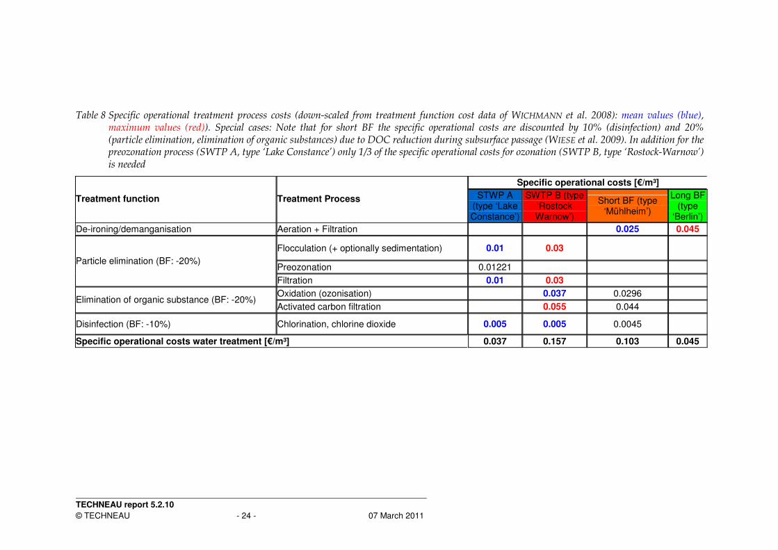
the CCA, the specific operational treatment costs are down-scaled to the underlying treatment processes as defined in Appendix A, Table 8. For this it is assumed that the specific operational treatment costs of BF are discounted by 10% (disinfection) and 20% (particle elimination, elimination of organic substance) compared to surface water treatment plants (SWTPs), due to the fact that BF acts as barrier against organic water constituents (WIESE et al. 2009) and suspended solids.

2.4 Static capital budgeting approach

Basically the methods of capital budgeting can be subdivided into static and dynamic methods. The difference between both methods is that dynamic methods consider temporal different incurring costs through accumulation and discounting, while static methods do not (LAWA 2005). Within this work the static capital budgeting approach is used, which requires the following simplifying assumptions:

- All investments are executed at the reference date (no accumulation needed) - Real costs and yield (reduced by inflation rate) are used instead of nominal costs/yield - No discounting for reinvestments necessary, since real costs are used!

The specific capital costs (€/m³) are calculated according to the following equation ( 2.4a):

mandageWaterDeAnnualAver

CostsInvestmentorenanceFactMa

mandageWaterDeAnnualAveronDurationDepreciati

alYieldCostsInvestmentmpitalCostsSpecificCa

onDurationDepreciati⋅

+⋅

+=

int)Re1(³]/[€

with:

- Investment costs [€]: of the respective water supply infrastructure (estimated in Chapter 2.3.2.1 and 2.3.2.2).

- Financial boundary conditions (as defined in Chapter 2.3.1.2) o Real yield [%] o Depreciation duration [a] o Maintenance factor [%]

- Annual average water demand [m³/a]: 10.000.000 m³ (as defined in Chapter 2.3.1) Note that the depreciation duration has to be equal with the assumed average lifetime of the investment, since a static capital budgeting approach is applied. If this prerequisite is not fulfilled (e.g. depreciation duration much shorter than the average lifetime of the investment) the capital cost assessment would lead to a wrong result since the capital costs have to be divided by the assumed depreciation duration for the specific capital cost calculation (here: shorter depreciation period will lead to increasing specific capital costs). Furthermore it has to be kept in mind that only costs for the water abstraction and water treatment processes are considered in the CCA. However the total cost structure of a waterworks includes much more cost types, for example costs for building sites or development (for details see Appendix A, Table 5). Thus the calculated specific capital costs (see Chapter 3.2) are much lower than they would be for a real waterworks (not shown). In case that only specific investment costs are calculated (i.e. for assessing the difference between specific capital and investment costs) the input parameters maintenance factor and real yield are not required, which leads to the following simplified equation ( 2.4b):

mandageWaterDeAnnualAveronDurationDepreciati

CostsInvestmentmstsvestmentCoSpecificIn

⋅=³]/[€



3 Results of comparative cost analysis

3.1 Cost estimate of investment and specific operational costs

The CCA is performed for a hypothetic waterworks treatment plant with a maximum daily capacity of 46.565 m³ and an annual average water production rate of 10 million m³. The considered cost types used in this analysis are limited to the two processes water abstraction and treatment, which are presented in detail in Appendix A, Table 6. Consequently this CCA does not cover all cost types of the considered water supply alternatives (see Appendix A, Table 5). Thus the results of the CCA are limited to conditions for which the neglected cost types are in the same order of magnitude for all alternatives.

3.1.1 Water abstraction

The costs for the water abstraction process are summarized in Table 2. It can be seen that both investment costs (-3.5 m €) and specific operational costs (-0.014 €/m³) are much lower in case of surface water abstraction. Consequently BF systems have a structural disadvantage compared to surface water. This can only be compensated through cost savings for the water treatment process, which is analysed in the following Chapter 3.1.2.

Table 2 Impact of water abstraction scenario on investment costs and specific operational costs for water abstraction process (input data, see Chapter 2.3.2.1)

Water abstraction scenario Investment costs [€] Specific operational costs [€/m³]

SW 837,448 0.006

GW (short BF, long BF) 4,291,494 0.020

3.1.2 Water treatment

The results for the water treatment costs estimation are illustrated in Table 3. Note that the lower the raw water quality, the higher are investment and specific operational costs. The very good raw water quality scenario (SWTP A, type ‘Lake Constance’) has the lowest investment and specific operational costs, however it is not directly comparable to the other scenarios since its surface water quality is very good whilst all others are evaluated as low (see also Table 1).

Table 3 Impact of raw water quality scenarios on investment costs and specific operational costs for water treatment (input data, see Chapter 2.3.2.2)

Scenario Surface water

quality Raw water

quality Investment

costs [€] Specific operational

costs [€/m³]

SWTP A (type ‘Lake Constance’) Very good Very good 6,901,423 0.037

SWTP B (type ‘Rostock-Warnow’) Low 20,658,928 0.157

Short BF (type ‘Mühlheim’) Medium 17,636,614 0.103

Long BF (type ‘Berlin’)

Low

Good 8,098,490 0.045



Nevertheless it is included as a reference scenario to assess the structural advantage of very good quality raw water on the water treatment costs. In case of long BF with good raw water quality this structural advantage is very low (difference in investment costs: +1.2 m €, specific operational costs: +0.008 €/m³) while it increases for short BF with medium raw water quality (difference in investment costs: +10.7 m €, operational costs: +0.066 €/m³) and is highest in case of SWTP B (type ‘Rostock-Warnow’) with low raw water quality (difference in investment costs: +13.7 m €, specific operational costs: +0.12 €/m³) In a nutshell, assuming equal surface water quality, BF systems provide treatment cost savings compared to the direct surface water treatment with low quality source water, since both investment and specific operational costs are lower. In addition long BF (minimum travel time > 50 days) provides a better raw water quality, which requires no advanced post-treatment (i.e. ozonation and activated carbon filtration) and thus is more cost efficient compared to short BF (minimum travel time < 10 days). However, whether these treatment cost savings are sufficient to compensate the structural disadvantage of higher water abstraction costs in case of BF (see Chapter 3.1.1) will be presented in Chapter 3.3.

3.2 Calculation of specific capital costs

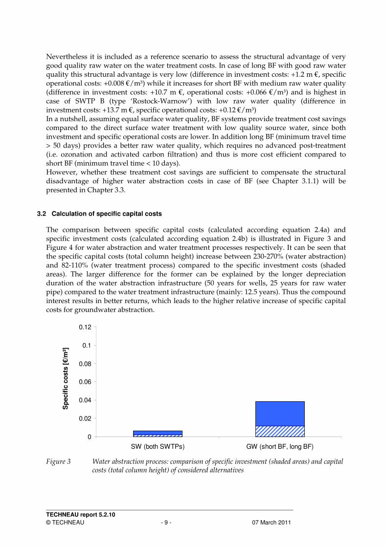
The comparison between specific capital costs (calculated according equation 2.4a) and specific investment costs (calculated according equation 2.4b) is illustrated in Figure 3 and Figure 4 for water abstraction and water treatment processes respectively. It can be seen that the specific capital costs (total column height) increase between 230-270% (water abstraction) and 82-110% (water treatment process) compared to the specific investment costs (shaded areas). The larger difference for the former can be explained by the longer depreciation duration of the water abstraction infrastructure (50 years for wells, 25 years for raw water pipe) compared to the water treatment infrastructure (mainly: 12.5 years). Thus the compound interest results in better returns, which leads to the higher relative increase of specific capital costs for groundwater abstraction.

0

0.02

0.04

0.06

0.08

0.1

0.12

SW (both SWTPs) GW (short BF, long BF)

Sp

ecif

ic c

osts

[€/m

³]

Figure 3 Water abstraction process: comparison of specific investment (shaded areas) and capital

costs (total column height) of considered alternatives



0

0.02

0.04

0.06

0.08

0.1

0.12

SWTP A

(type 'Lake

Constance')

SWTP B

(type 'Rostock-

Warnow')

short BF

(type 'Mühlheim')

long BF

(type 'Berlin')

Sp

ecif

ic c

osts

[€/m

³]

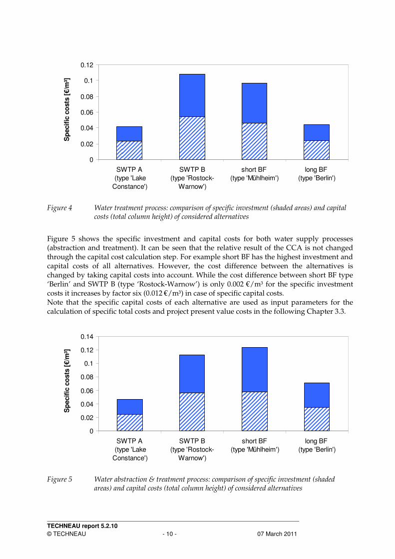
Figure 4 Water treatment process: comparison of specific investment (shaded areas) and capital

costs (total column height) of considered alternatives

Figure 5 shows the specific investment and capital costs for both water supply processes (abstraction and treatment). It can be seen that the relative result of the CCA is not changed through the capital cost calculation step. For example short BF has the highest investment and capital costs of all alternatives. However, the cost difference between the alternatives is changed by taking capital costs into account. While the cost difference between short BF type ‘Berlin’ and SWTP B (type ‘Rostock-Warnow’) is only 0.002 €/m³ for the specific investment costs it increases by factor six (0.012 €/m³) in case of specific capital costs. Note that the specific capital costs of each alternative are used as input parameters for the calculation of specific total costs and project present value costs in the following Chapter 3.3.

0

0.02

0.04

0.06

0.08

0.1

0.12

0.14

SWTP A

(type 'Lake

Constance')

SWTP B

(type 'Rostock-

Warnow')

short BF

(type 'Mühlheim')

long BF

(type 'Berlin')

Sp

ecif

ic c

osts

[€/m

³]

Figure 5 Water abstraction & treatment process: comparison of specific investment (shaded

areas) and capital costs (total column height) of considered alternatives



3.3 Specific total costs and project present value costs

The specific total costs (left y-axis) and the project present value costs (right y-axis) for the four considered alternatives are shown in Figure 6. Note that the specific total costs are the sum of the specific operational costs (estimated in Chapters 3.1.1 and 3.1.2.) and the specific capital costs (see Chapter 3.2). The project present value costs are calculated by multiplying the specific total costs with the average annual water demand (10 Mio m³) and the examination period (50 years) which is equal with the assumed lifetime of the waterworks.

0.00

0.05

0.10

0.15

0.20

0.25

0.30

SWTP A

(type 'Lake

Constance')

SWTP B

(type 'Rostock-

Warnow')

Short BF

(type 'Mühlheim')

Long BF

(type 'Berlin')

Sp

ecif

ic t

ota

l co

sts

[€/m

³]

0

20

40

60

80

100

120

140

Pro

ject

pre

sen

t valu

e c

osts

[m

€]

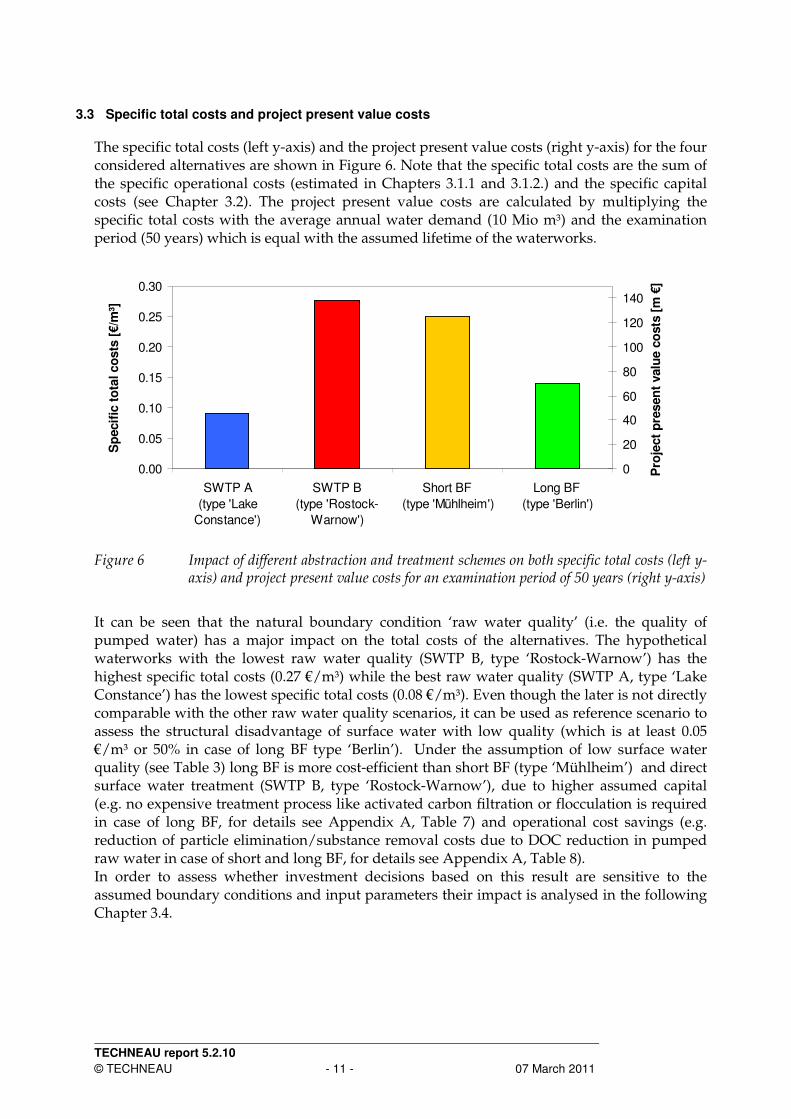
Figure 6 Impact of different abstraction and treatment schemes on both specific total costs (left y-

axis) and project present value costs for an examination period of 50 years (right y-axis)

It can be seen that the natural boundary condition ‘raw water quality’ (i.e. the quality of pumped water) has a major impact on the total costs of the alternatives. The hypothetical waterworks with the lowest raw water quality (SWTP B, type ‘Rostock-Warnow’) has the highest specific total costs (0.27 €/m³) while the best raw water quality (SWTP A, type ‘Lake Constance’) has the lowest specific total costs (0.08 €/m³). Even though the later is not directly comparable with the other raw water quality scenarios, it can be used as reference scenario to assess the structural disadvantage of surface water with low quality (which is at least 0.05 €/m³ or 50% in case of long BF type ‘Berlin’). Under the assumption of low surface water quality (see Table 3) long BF is more cost-efficient than short BF (type ‘Mühlheim’) and direct surface water treatment (SWTP B, type ‘Rostock-Warnow’), due to higher assumed capital (e.g. no expensive treatment process like activated carbon filtration or flocculation is required in case of long BF, for details see Appendix A, Table 7) and operational cost savings (e.g. reduction of particle elimination/substance removal costs due to DOC reduction in pumped raw water in case of short and long BF, for details see Appendix A, Table 8). In order to assess whether investment decisions based on this result are sensitive to the assumed boundary conditions and input parameters their impact is analysed in the following Chapter 3.4.



3.4 Sensitivity and scenario analysis

A sensitivity analysis is carried out in order to assess the impact of varying technical (Chapter 3.4.1) and financial boundary conditions (Chapter 3.4.2) on the the cost-efficiency of BF compared to direct surface water treatment. In addition a scenario analysis (Chapter 3.4.3) is performed to assess the impact of the higher monitoring demand for groundwater abstractions in case of BF systems.

3.4.1 Technical boundary conditions

The impact of the technical boundary condition ‘average pumping rate per production well’ on the specific total costs is given in Figure 7. If the pumping rate is lowered by factor ten (compared to the reference scenario: 100 m³/h) the number of production wells has to increase by factor ten so that the same quantity of raw water can be delivered. Consequently the specific capital costs for water abstraction increase by 0.10 €/m³. Nevertheless the total costs of long BF (type ’Berlin’) are still 0.04 €/m³ below the total costs of the SWTP B (type ‘Rostock-Warnow). However in case of short BF (type ‘Mühlheim’) there is a critical pumping rate of about 26 m³/h (break-even-point) which needs to be exceeded so that BF is more cost-efficient than the SWTP B (type ’Rostock-Warnow’). Note that in this calculation the lifting height remains constant for all pumping rates, which is an unrealistic assumption since pumping rate and lifting height are inversely dependent. However neglecting this dependency has only a minor impact on the CCA result since the portion of pumping costs for BF accounts only 0.02 €/m³ (see Table 2) of the specific total costs. Consequently, if the pumping rate per well is at least reduced to 40 m³/h the increased capital costs (≥ 0.017 €/m³) for the additional production wells can never be fully compensated by potential pumping cost savings.

0.00

0.05

0.10

0.15

0.20

0.25

0.30

0.35

0.40

10 20 30 40 50 60 70 80 90 100

Pumping rate per well [m³/h]

Sp

ecif

ic t

ota

l co

sts

[€/m

³]

Long BF (type 'Berlin') SWTP A (type 'Lake Constance')

Short BF (type 'Mühlheim') SWTP B (type 'Rostock-Warnow')

Figure 7 Impact of varying pumping rate per production well on the cost-efficiency of BF



3.4.2 Financial boundary conditions

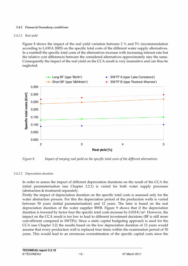
3.4.2.1 Real yield Figure 8 shows the impact of the real yield variation between 2 % and 5% (recommendation according to LAWA 2005) on the specific total costs of the different water supply alternatives. In a nutshell the specific total costs of the alternatives increase with increasing interest rate but the relative cost differences between the considered alternatives approximately stay the same. Consequently the impact of the real yield on the CCA result is very insensitive and can thus be neglected.

0.000

0.050

0.100

0.150

0.200

0.250

0.300

0.350

2 3 4 5

Real yield [%]

Sp

ecif

ic t

ota

l co

sts

[€/m

³]



Figure 8 Impact of varying real yield on the specific total costs of the different alternatives

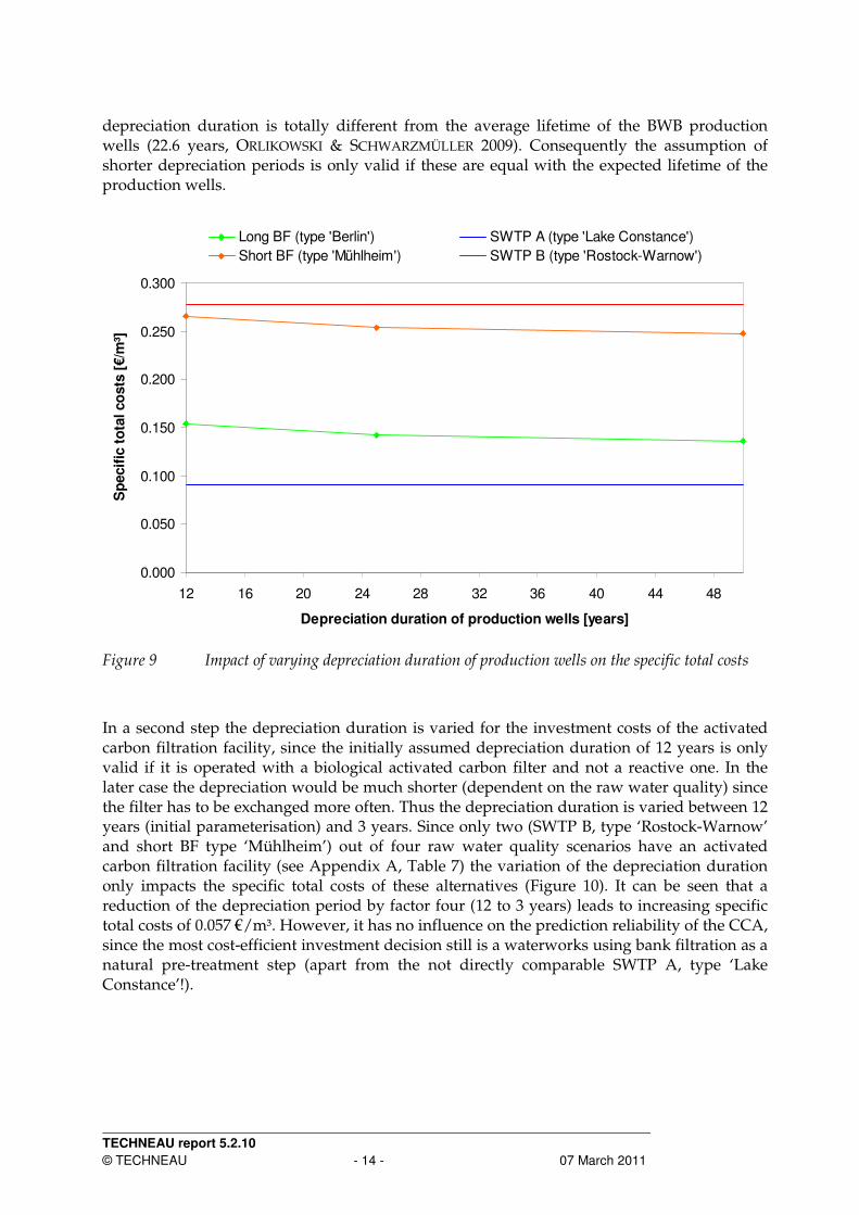
3.4.2.2 Depreciation duration In order to assess the impact of different depreciation durations on the result of the CCA the initial parameterisation (see Chapter 2.2.1) is varied for both water supply processes (abstraction & treatment) separately. Firstly the impact of depreciation duration on the specific total costs is assessed only for the water abstraction process. For this the depreciation period of the production wells is varied between 50 years (initial parameterisation) and 12 years. The later is based on the real depreciation duration of the water supplier BWB. Figure 9 shows that if the depreciation duration is lowered by factor four the specific total costs increase by 0.018 €/m³. However, the impact on the CCA result is too low to lead to different investment decisions (BF is still more cost-efficient compared to SWTPs). Since a static capital budgeting approach is used for the CCA (see Chapter 3.2) the results based on the low depreciation duration of 12 years would assume that every production well is replaced four times within the examination period of 50 years. This would lead to an erroneous overestimation of the specific capital costs since the



depreciation duration is totally different from the average lifetime of the BWB production wells (22.6 years, ORLIKOWSKI & SCHWARZMÜLLER 2009). Consequently the assumption of shorter depreciation periods is only valid if these are equal with the expected lifetime of the production wells.

0.000

0.050

0.100

0.150

0.200

0.250

0.300

12 16 20 24 28 32 36 40 44 48

Depreciation duration of production wells [years]

Sp

ecif

ic t

ota

l co

sts

[€/m

³]



Figure 9 Impact of varying depreciation duration of production wells on the specific total costs

In a second step the depreciation duration is varied for the investment costs of the activated carbon filtration facility, since the initially assumed depreciation duration of 12 years is only valid if it is operated with a biological activated carbon filter and not a reactive one. In the later case the depreciation would be much shorter (dependent on the raw water quality) since the filter has to be exchanged more often. Thus the depreciation duration is varied between 12 years (initial parameterisation) and 3 years. Since only two (SWTP B, type ‘Rostock-Warnow’ and short BF type ‘Mühlheim’) out of four raw water quality scenarios have an activated carbon filtration facility (see Appendix A, Table 7) the variation of the depreciation duration only impacts the specific total costs of these alternatives (Figure 10). It can be seen that a reduction of the depreciation period by factor four (12 to 3 years) leads to increasing specific total costs of 0.057 €/m³. However, it has no influence on the prediction reliability of the CCA, since the most cost-efficient investment decision still is a waterworks using bank filtration as a natural pre-treatment step (apart from the not directly comparable SWTP A, type ‘Lake Constance’!).



0.000

0.100

0.200

0.300

0.400

0.500

0.600

3 4 5 6 7 8 9 10 11 12

Depreciation duration of ACF facility [years]

Sp

ecif

ic t

ota

l co

sts

[€/m

³]



Figure 10 Impact of varying depreciation duration of activated carbon filtration (ACF) facility on

specific total costs

3.4.3 Monitoring scenario analysis

The monitoring scenario analysis is based on the same boundary conditions (water demand and water availability) as defined in Chapter 2.2.1. However, the impact of the monitoring demand for surface water and groundwater abstractions is included in the analysis since there is a large systematic difference between them:

- Higher investment costs need to be taken into account for additional monitoring wells in case of BF systems

- Higher sampling frequency in case of SW abstractions due to higher temporal variability of surface water quality.

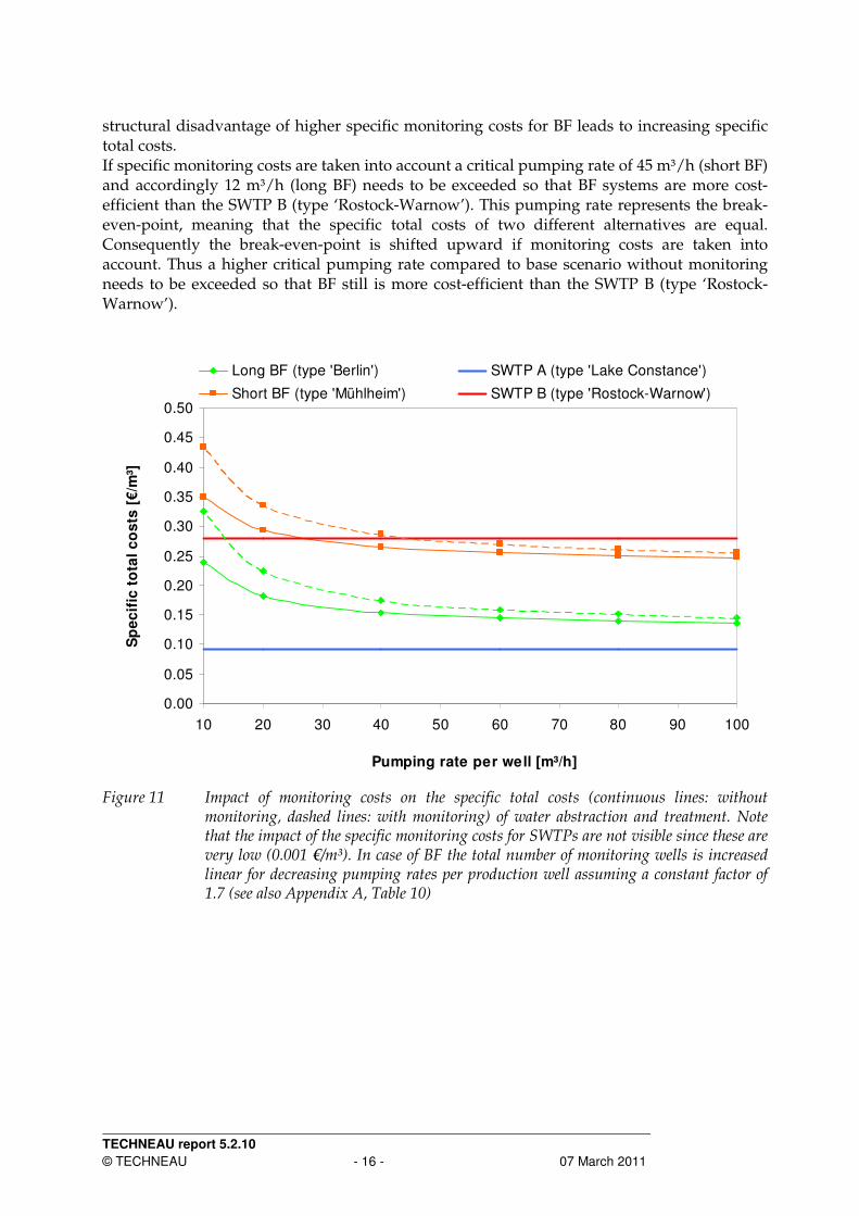
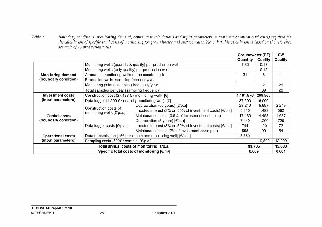
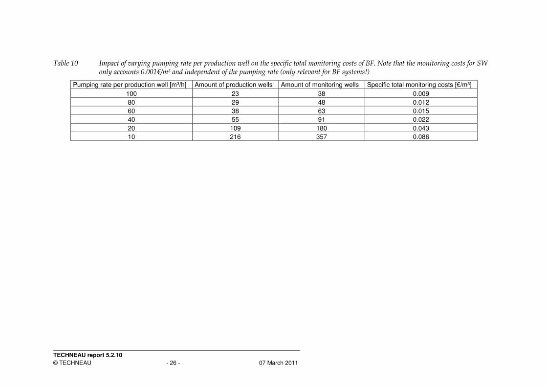
The assumed boundary conditions and input parameters (investment & operational costs) for the monitoring scenario are listed in Appendix A, Table 9. The result of the monitoring scenario analysis on the specific total costs (dashed lines: with monitoring, continuous lines: without monitoring) for the four considered alternatives is shown in Figure 11. In addition the impact of varying pumping rates per production well on the specific monitoring costs is also considered in the framework of a sensitivity analysis (assuming a constant factor of monitoring wells per production well, see Appendix A, Table 9). Note that the assumption of a constant factor ‘monitoring wells per production well’ may not be appropriate. For example less monitoring wells are needed for very compact well fields, while the opposite is the case for long ranging well fields (e.g. in different subsurface catchments). In case of SWTPs the impact of monitoring costs on the specific total costs is very low (0.001 €/m³) and thus not visible in Figure 11. However, for groundwater abstractions (BF systems) the specific monitoring costs account 0.009 €/m³ for a pumping rate of 100 m³/h and 0.086 €/m³ for a pumping rate of 10 m³/h (see Appendix A, Table 10 for detailed calculation). This



structural disadvantage of higher specific monitoring costs for BF leads to increasing specific total costs. If specific monitoring costs are taken into account a critical pumping rate of 45 m³/h (short BF) and accordingly 12 m³/h (long BF) needs to be exceeded so that BF systems are more cost-efficient than the SWTP B (type ‘Rostock-Warnow’). This pumping rate represents the break-even-point, meaning that the specific total costs of two different alternatives are equal. Consequently the break-even-point is shifted upward if monitoring costs are taken into account. Thus a higher critical pumping rate compared to base scenario without monitoring needs to be exceeded so that BF still is more cost-efficient than the SWTP B (type ‘Rostock-Warnow’).

0.00

0.05

0.10

0.15

0.20

0.25

0.30

0.35

0.40

0.45

0.50

10 20 30 40 50 60 70 80 90 100

Pumping rate per well [m³/h]

Sp

ec

ific

to

tal

co

sts

[€

/m³]



Figure 11 Impact of monitoring costs on the specific total costs (continuous lines: without

monitoring, dashed lines: with monitoring) of water abstraction and treatment. Note that the impact of the specific monitoring costs for SWTPs are not visible since these are very low (0.001 €/m³). In case of BF the total number of monitoring wells is increased linear for decreasing pumping rates per production well assuming a constant factor of 1.7 (see also Appendix A, Table 10)



4 Conclusions

In general water suppliers prefer water sources that yield the best water quality and security under the constraint of guaranteeing a sufficient water availability according the following descending order (MUTSCHMANN & STIMMELMAYR 2007):

1. Groundwater, without treatment 2. Groundwater, with treatment 3. Groundwater, with artificial recharge (BF or MAR) 4. Drinking water reservoir 5. Lake water 6. River water

The considered water source alternatives for the CCA documented in this report are limited to groundwater with artificial recharge (BF systems) and surface water from lakes (SWTP A, type ‘Lake Constance’) or rivers (SWTP B, type ‘Rostock-Warnow’). Under the assumption of equally low surface water quality the CCA for the water supply processes abstraction and treatment yielded that BF systems are more cost-efficient than SWTPs (see Chapter 3.3), which is in line with the water suppliers water source priority stated above. On the one hand surface water abstractions are more cost-efficient compared to BF systems for the water abstraction process (see Chapter 3.1.1). On the other hand this initial benefit is overcompensated in case of low raw water quality (SWTP B, type ‘Rostock-Warnow’), leading to higher treatment costs compared to both BF systems with medium (short BF, <10d) or good (long BF, >50d) raw water quality (see Chapter 3.1.2). Furthermore the sensitivity analysis confirmed that the natural boundary condition ‘pumping rate per production well’, which is determined by the hydrogeological setting, has a major impact on the specific total costs of BF systems (see Chapter 3.4.1). The lower the ‘pumping rate per well’ (varied between 100 m³/h and 10 m³/h) the more production wells are needed to deliver the required raw water, which leads to increasing capital costs for the additional wells (up to 0.10 €/m³). Consequently, short BF is only more cost efficient compared to direct surface water use (SWTP B, type ‘Rostock-Warnow’) if the pumping rate per well stays above a critical value of 16 m³/h, while in case of long BF no critical value is identified. In addition the result of the monitoring scenario analysis clearly confirmed that for this aspect groundwater waterworks have a structural disadvantage compared to surface waterworks, which varies between 0.008 and 0.085 €/m³ (depending on the amount of monitoring wells, see Appendix A, Table 10). Subsequently, if monitoring costs are taken into account, a higher critical pumping rate per production well (short BF: 45 m³/h, long BF: 12 m³/h) is required to exceed the break-even-point compared to the base case without monitoring (short BF: 16m³/h, long BF: no critical pumping rate identified) As usual, the results of the CCA are limited by the input data quality that is used for the assessment. While investment costs are estimated relatively easy on process scale for both water abstraction and treatment this was not possible for the specific operational costs, which are aggregated either on waterworks (energy demand: BWB data) or functional scale (treatment: WICHMANN et al. 2008). Subsequently it is difficult to assign them to the underlying processes properly, which restricts the prediction reliability of the CCA. Furthermore the application of the CCA is only adequate if the methodological prerequisites are fulfilled. Since the CCA is a fully cost orientated evaluation method it is a prerequisite that the total cost structure of each alternative is considered, which is not the case within this work (see Appendix A, Table 5).



In addition the prerequisite of benefit equity of the considered alternatives is not fulfilled, since BF provides unconsidered added values compared to direct surface water use:

• Temporal mitigation of abstraction impact on surface water bodies (see e.g. BREDEHOEFT & KENDY 2008)

• Improved source water reliability (RAY et al. 2002)

Nevertheless the CCA results are valid as long as BF is the most cost-efficient solution and the unconsidered cost types are in the same order of magnitude for all alternatives (e.g. costs for building sites or development). Within these assumptions the CCA is a valuable tool for water supply managers in the complex process of making rational investment decisions. However, if the above stated prerequisites and exceptions are not fulfilled (e.g. critical pumping rate per production well is not exceeded, see Chapter 3.4.1 and 3.4.3), the CCA is only a first step in the economic assessment and more powerful evaluation methods (e.g. cost-benefit analysis) are needed. In a nutshell it needs to be stated that in case of poor surface water quality, taking water abstraction and water treatment processes into account BF usually yields lower total costs compared to direct surface water use. On the other hand, there may be no cost benefit in cases of very good surface water quality (i.e. less treatment necessary) or unfavourable hydrogeological settings (i.e. low aquifer yield). However, even in this case there might still be unconsidered non-monetary benefits (e.g. additional safety barrier for hazardous substances, higher source water reliability) that might outweigh the higher costs identified within this study.



Appendix A

Table 4 Comparison of basic evaluation methods for cost-benefit analysis by means of a general method model, translated from LAWA (2005)

Evaluation method

Task

Comparative cost analysis

Extended comparative cost analysis

Cost-benefit analysis Value benefit analysis Cost effectiveness analysis

Combinations and open evaluation methods

1. Problem definition

Working steps for the preliminary clarification of the task are performed according to the purpose of analysis, scope and complexity of methods as well as to determination of the predefined target

Macroeconomic / microeconomic cost effects

Ascertainment of target system, analytical evaluation with regard to

(Prerequisite: benefit equity)

+ economic difference benefit between alternatives

Economic efficiency (in terms of macroeconomy, regionality etc.)

Target system to be developed for specific problem areas

Cost effects to be integrated and target system to be developed for specific problem areas

In the most comprehensive case: macroeconomic efficiency, environmental quality, regional development, social welfare

2.

Target emphasis No longer required Target emphasis for all target criteria In certain sub-areas

3. Determination of decision field

No method-specific differences

4. Pre-selection of further measures to be analysed

Pr

eli

min

ar

y s

ta

ge

No method-specific differences

Input causing costs 5. Determination of the decision relevant method impacts (impact analysis)

+ difference gains between the alternatives

Required quantities, quantitative gains and savings

Target gains Input causing costs + target gains

In the most comprehensive case: all positive and negative (quantity) effects

6. Definition of the measurement scale and parameters

Ratio scale for monetary units

Striving for cardinal scales for non-monetary units

Cost effective disadvantages like cost comparison, extended cost comparison, cost-benefit analysis Advantages and other disadvantages like value benefit analysis

Different scales, monetary and non-monetary units

7. Evaluation of method impacts

Cost series Cost series and series of difference benefit

Cost and benefit series Target values Cost series and target values

Cost and benefit series, target values, indicators

8. Cost-Benefit comparison

Mo

re

s

pe

cif

ic a

na

lys

is

Not required, only comparison of cost cash values and annual cost respectively

In parts: comparison of cost cash values by calculating difference benefit cash values

Comparison of the capital values or benefit-cost ration (problem-independent!)

Comparison of benefit values

Application of the principle of efficiency and economy or comparison of benefit-cost ration (problem-dependent!)

Partial balancing, comparison of target earnings and renunciation (trade-offs)



Evaluation method

Absolute statement Relative statement Delivers in view of evaluation target (step 2)

Relative statement on the advantageousness in case of mutually exclusive alternatives in case of mutually exclusive and non exclusive alternatives

Relative statement as mentioned alongside or open

9. Sensitivity check

Limiting the uncertainty and risk factors in the calculations of steps 6 and 7 as well as in the calculation hypothesis in step 8 and their impacts on the results of step 8. Determination of critical values; differences in processing immediately result from type and scope of input data of the steps mentioned.

10. Demonstration of non-ascertainable method impact

Intangible costs, monetary and non-monetary benefit differences

Intangible costs and benefit differences

Intangible and extra economic impacts

Not required Model-theoretic

Not required Model-theoretic

In individual partial balances, according to the particular linking of evaluation methods

11. Overall evaluation of methods

Joining the partial results from steps 8 and 9 with those of step 10 into a complete edition

Development of a complete edition based on the results from step 8 including the findings from step 9

For open methods Preparation of the results for the coordination process

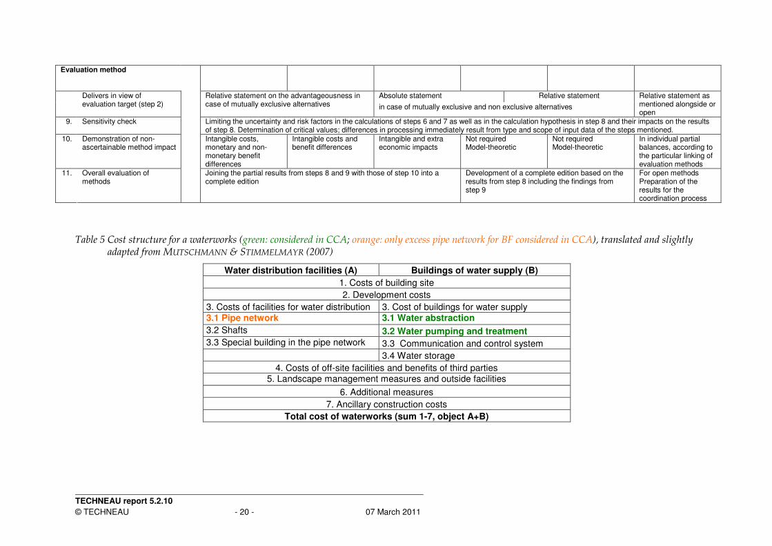
Table 5 Cost structure for a waterworks (green: considered in CCA; orange: only excess pipe network for BF considered in CCA), translated and slightly adapted from MUTSCHMANN & STIMMELMAYR (2007)

Water distribution facilities (A) Buildings of water supply (B)

1. Costs of building site

2. Development costs

3. Costs of facilities for water distribution 3. Cost of buildings for water supply 3.1 Pipe network 3.1 Water abstraction

3.2 Shafts 3.2 Water pumping and treatment

3.3 Special building in the pipe network 3.3 Communication and control system

3.4 Water storage

4. Costs of off-site facilities and benefits of third parties 5. Landscape management measures and outside facilities

6. Additional measures

7. Ancillary construction costs

Total cost of waterworks (sum 1-7, object A+B)



Table 6 Classification of specific total costs for water abstraction and treatment to cost units and cost type (slightly adapted from HOLLÄNDER et

al. 2009) and considered cost types in CCA (unconsidered cost types are marked in red)

Cost units to primary processes Cost type (rough classification)

Cost type (precise classification)

Cost types and parameters considered in

CCA

Depreciation √√√√ (wells: 50 years)

Imputed interest √√√√ (real yield: 3% on 50% of investment costs)

Specific capital costs water abstraction [€/m³]

Maintenance √√√√ (2% of investment costs)

Staff

Energy and material costs √√√√ (only electrical energy costs!)

Specific costs water abstraction [€/m³]

Specific operating costs water abstraction [€/m³]

Other operating costs

Depreciation √√√√ (buildings, equipment filters: 12.5 years)

Imputed interest √√√√ (real yield: 3% on 50% of investment costs)

Specific capital costs water treatment [€/m³]

Maintenance √√√√ (0.5% for buildings and 2% of investment costs)

Staff

Energy and material costs

Sp

ecif

ic t

ota

l co

sts

[€/m

³]

Specific costs water treatment [€/m³]

Specific operating costs water treatment [€/m³]

Other operating costs

√√√√ (only rough classification),

precise classification is only available for

flocculation at SWTP Spandau



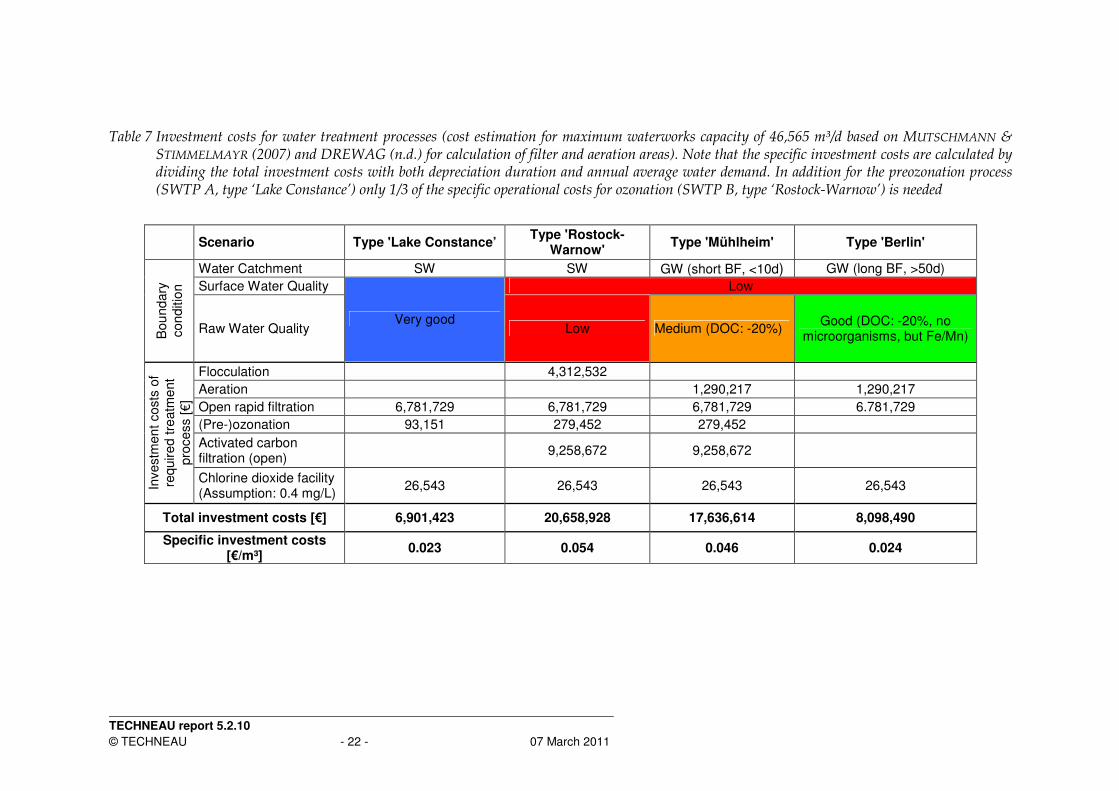
Table 7 Investment costs for water treatment processes (cost estimation for maximum waterworks capacity of 46,565 m³/d based on MUTSCHMANN & STIMMELMAYR (2007) and DREWAG (n.d.) for calculation of filter and aeration areas). Note that the specific investment costs are calculated by dividing the total investment costs with both depreciation duration and annual average water demand. In addition for the preozonation process (SWTP A, type ‘Lake Constance’) only 1/3 of the specific operational costs for ozonation (SWTP B, type ‘Rostock-Warnow’) is needed

Scenario Type 'Lake Constance’ Type 'Rostock-

Warnow' Type 'Mühlheim' Type 'Berlin'

Water Catchment SW SW GW (short BF, <10d) GW (long BF, >50d)

Surface Water Quality Low

Bou

ndary

conditio

n

Raw Water Quality Very good

Low Medium (DOC: -20%) Good (DOC: -20%, no

microorganisms, but Fe/Mn)

Flocculation 4,312,532

Aeration 1,290,217 1,290,217

Open rapid filtration 6,781,729 6,781,729 6,781,729 6.781,729

(Pre-)ozonation 93,151 279,452 279,452

Activated carbon filtration (open)

9,258,672 9,258,672

Investm

en

t costs

of

require

d tre

atm

ent

pro

cess [€]

Chlorine dioxide facility (Assumption: 0.4 mg/L)

26,543 26,543 26,543 26,543

Total investment costs [€] 6,901,423 20,658,928 17,636,614 8,098,490

Specific investment costs [€/m³]

0.023 0.054 0.046 0.024



0 €

1,000,000 €

2,000,000 €

3,000,000 €

4,000,000 €

5,000,000 €

6,000,000 €

7,000,000 €

8,000,000 €

Flocculation Aeration Rapid filtration

(open)

Ozonisation Activated carbon

filtration (open)

Chorine dioxide

facility

Investm

en

t co

sts

[€]

Construction costs Filter costs Equipment Total investment costs

Figure 12 Detailed investment cost structure (construction, filter, equipment) for considered treatment processes. Investment cost estimation for

maximum waterworks capacity of 46,565 m³/d, based on Mutschmann & Stimmelmayr (2007) and DREWAG (n.d.) for calculation of filter and aeration areas.



Table 8 Specific operational treatment process costs (down-scaled from treatment function cost data of WICHMANN et al. 2008): mean values (blue), maximum values (red)). Special cases: Note that for short BF the specific operational costs are discounted by 10% (disinfection) and 20% (particle elimination, elimination of organic substances) due to DOC reduction during subsurface passage (WIESE et al. 2009). In addition for the preozonation process (SWTP A, type ‘Lake Constance’) only 1/3 of the specific operational costs for ozonation (SWTP B, type ‘Rostock-Warnow’) is needed

Specific operational costs [€/m³]

Treatment function Treatment Process STWP A (type ‘Lake Constance’)

SWTP B (type ‘Rostock Warnow’)

Short BF (type ‘Mühlheim’)

Long BF (type

‘Berlin’)

De-ironing/demanganisation Aeration + Filtration 0.025 0.045

Flocculation (+ optionally sedimentation) 0.01 0.03

Preozonation 0.01221 Particle elimination (BF: -20%)

Filtration 0.01 0.03

Oxidation (ozonisation) 0.037 0.0296 Elimination of organic substance (BF: -20%)

Activated carbon filtration 0.055 0.044

Disinfection (BF: -10%) Chlorination, chlorine dioxide 0.005 0.005 0.0045

Specific operational costs water treatment [€/m³] 0.037 0.157 0.103 0.045



Table 9 Boundary conditions (monitoring demand, capital cost calculation) and input parameters (investment & operational costs) required for the calculation of specific total costs of monitoring for groundwater and surface water. Note that this calculation is based on the reference scenario of 23 production wells

Groundwater (BF) SW

Quantity Quality Quality

Monitoring wells (quantity & quality) per production well 1.32 0.18

Monitoring wells (only quality) per production well 0.15

Amount of monitoring wells (to be constructed) 31 8 1

Production wells: sampling frequency/year 1

Monitoring points: sampling frequency/year 2 26

Monitoring demand (boundary condition)

Total samples per year (sampling frequency 39 26

Construction cost (37,483 € / monitoring well) [€] 1,161,976 299,865 Investment costs (input parameters) Data logger (1,200 € / quantity monitoring well) [€] 37,200 6,000

Depreciation (50 years) [€/p.a] 23,240 5,997 2,249

Imputed interest (3% on 50% of investment costs) [€/p.a] 5,810 1,499 562 Construction costs of monitoring wells [€/p.a.]

Maintenance costs (0.5% of investment costs p.a.) 17,430 4,498 1,687

Depreciation (5 years) [€/p.a] 7,440 1,200 720

Imputed interest (3% on 50% of investment costs) [€/p.a] 744 120 72

Capital costs (boundary condition)

Data logger costs [€/p.a.]

Maintenance costs (2% of investment costs p.a.) 558 90 54

Data transmission (15€ per month and monitoring well) [€/p.a.] 5,580 Operational costs (input parameters) Sampling costs (500€ / sample) [€/p.a.] 19,500 13,000

Total annual costs of monitoring [€/p.a.] 93,706 13,000

Specific total costs of monitoring [€/m³] 0.009 0.001



Table 10 Impact of varying pumping rate per production well on the specific total monitoring costs of BF. Note that the monitoring costs for SW only accounts 0.001€/m³ and independent of the pumping rate (only relevant for BF systems!)

Pumping rate per production well [m³/h] Amount of production wells Amount of monitoring wells Specific total monitoring costs [€/m³]

100 23 38 0.009

80 29 48 0.012

60 38 63 0.015

40 55 91 0.022

20 109 180 0.043

10 216 357 0.086



5 References

BREDEHOEFT, J. & KENDY, E. (2008): Strategies for offsetting seasonal impacts of pumping on a nearby stream Ground Water 46(1): 23-29 CHAWEZA, D. P. (2006): Feasability of riverbank filtration for water treatment in selected cities of Malawi, UNESCO-IHE. MSc DREWAG (n.d.): Wasserwerk Dresden-Hosterwitz: 8 p., http://www.drewag.de/media/pdf/de/drewag_treff_infomaterial/info_hosterwitz_08.pdf HOLLÄNDER, R.; FÄLSCH, M.; GEYLER, S. & LAUTENSCHLÄGER, S. (2009): Trinkwasserpreise in Deutschland - Wie lassen sich verschiedene Rahmenbedingungen für die Wasserversorgung anhand von Indikatoren abbilden?: 71 p. KRINGS, S. & DÜLLMANN, H. (2002): Grundwasserproblematik im Stadtgebiet Korschenbroich - Konzeptentwicklung und gutachtliche Bewertung von langfristigen Lösungen zur Abwendung von Gebäudeschäden, Geotechnisches Büro Prof. Dr.-Ing. H. Düllmann: 85, http://www.korschenbroich.de/downloads/pdf/publikationen/Grundwassergutachten_Duellmann_1202.pdf http://www.korschenbroich.de/downloads/pdf/publikationen/Grundwassergutachten_Du

ellmann_1202_Kostenvariante3.pdf http://www.korschenbroich.de/downloads/pdf/publikationen/Grundwassergutachten_Du

ellmann_1202_Kostenvariante4.pdf LAWA (2005): Leitlinien zur Durchführung dynamischer Kostenvergleichsrechnungen (KVR-Leitlinien), Länderarbeitsgemeinschaft Wasser. MÖLLER, K. & BURGSCHWEIGER, J. (2008): Wasserversorgungskonzept für Berlin und für das von den BWB versorgte Umland (Entwicklung bis 2040), Berliner Wasserbetriebe: 85 p., http://www.berlin.de/sen/umwelt/wasser/grundwasser/de/wvk2040.shtml MUTSCHMANN, J. & STIMMELMAYR, F. (2007): Taschenbuch der Wasserversorgung. Wiesbaden, Friedr. Vieweg & Sohn Verlag | GWV Fachverlage GmbH Wiesbaden. ORLIKOWSKI, D. & SCHWARZMÜLLER, H. (2009): Advanced statistical analyses of well data. Project: Wellma-1. Berlin, Kompetenzzentrum Wasser Berlin (unveröffentlicht) RAY, C.; SCHUBERT, J.; MELIN, G. & LINSKY, R. B. (2002): Introduction. Riverbank Filtration - Improving Source-Water Quality. Chittaranjan, R.; Melin, G. & Linsky, R. B., Kluwer Academic Press: p. 1-18. SHAMRUKH, M. & ABDEL-WAHAB, A. (2008): Riverbank filtration for sustainable water supply: application to a large-scale facility on the Nile River Clean Technologies and Environmental Policy, http://dx.doi.org/10.1007/s10098-007-0143-2 TRINKWV (2001): Trinkwasserverordnung vom 21. Mai 2001 ('Drinking Water Ordinance'). http://bundesrecht.juris.de/bundesrecht/trinkwv_2001/



WICHMANN, K.; HEIN, A.; MÖLLER, K. & LÉVAI, P. (2008): Bewertung der technischen Prozesse in Wasserwirtschaft, -gewinnung und -aufbereitung. Prozesskennzahlen und Benchmarking: Perspektiven einer nachhaltigen Wasserwirtschaft (21. Mühlheimer Wassertechnisches Seminar, 6. März 2008), Berichte aus dem IWW - Rheinisch-Westfälisches Institut für Wasserforschung gGmbH. vol. 47: 27-50. WIESE, B.; ORLIKOWSKI, D.; HÜLSHOFF, I. & GRÜTZMACHER, G. (2009): Removal of 38 organic water constitutents by bank filtration in Berlin. Berlin, KompetenzZentrum Wasser Berlin

WP5.2: Combination of MAR and adjusted conventional ...

Documents

Transcript of WP5.2: Combination of MAR and adjusted conventional ...