World Happiness Report | EUR
172
World Happiness Report 2018 John F. Helliwell, Richard Layard and Jeffrey D. Sachs
Transcript of World Happiness Report | EUR
World Happiness Report
2018
John F. Helliwell, Richard Layard and Jeffrey D. Sachs

The World Happiness Report was written by a group of independent experts acting in their personal capacities. Any views expressed in this report do not necessarily reflect the views of any organization, agency or programme of the United Nations.
Table of Contents
World Happiness Report 2018Editors: John F. Helliwell, Richard Layard, and Jeffrey D. Sachs Associate Editors: Jan-Emmanuel De Neve, Haifang Huang and Shun Wang
1 Happiness and Migration: An Overview . . . . . . . . . . . . . . . . . . . 3 John F. Helliwell, Richard Layard and Jeffrey D. Sachs
2 International Migration and World Happiness . . . . . . . . . . . . . .13 John F. Helliwell, Haifang Huang, Shun Wang and Hugh Shiplett
3 Do International Migrants Increase Their Happiness and That of Their Families by Migrating? . . . . . . . . . . . . . . . . . 45 Martijn Hendriks, Martijn J. Burger, Julie Ray and Neli Esipova
4 Rural-Urban Migration and Happiness in China . . . . . . . . . . . . 67
John Knight and Ramani Gunatilaka
5 Happiness and International Migration in Latin America . . . . . . . . . . . . . . . . . . . . . . . . . . . . . . . . . . . . . . . . 89 Carol Graham and Milena Nikolova
6 Happiness in Latin America Has Social Foundations . . . . . . . 115
Mariano Rojas
7 America’s Health Crisis and the Easterlin Paradox . . . . . . . . 146
Jeffrey D. Sachs
Annex: Migrant Acceptance Index: Do Migrants Have Better Lives in Countries That Accept Them? . . . . . . . . . . . . . . . . . 160 Neli Esipova, Julie Ray, John Fleming and Anita Pugliese


2
3Chapter 1
Happiness and Migration: An Overview
John F. Helliwell, Vancouver School of Economics at the University of British Columbia, and Canadian Institute for Advanced Research
Richard Layard, Wellbeing Programme, Centre for Economic Performance, at the London School of Economics and Political Science
Jeffrey D. Sachs, Director, SDSN, and Director, Center for Sustainable Development, Columbia University
The authors are grateful to the Ernesto Illy Foundation and the Canadian Institute for Advanced Research for research support, and to Gallup for data access and assistance. The authors are also grateful for helpful advice and comments from Claire Bulger, Jan-Emmanuel De Neve, Neli Esposito, Carol Graham, Jon Hall, Martijn Hendricks, Haifang Huang, Marie McAuliffe, Julie Ray, Martin Ruhs, and Shun Wang.

World Happiness Report 2018
Increasingly, with globalisation, the people of
the world are on the move; and most of these
migrants are seeking a happier life. But do they
achieve it? That is the central issue considered
in this 2018 World Happiness Report.
But what if they do? The migrants are not the
only people affected by their decision to move.
Two other major groups of people are affected
by migration:
• those left behind in the area of origin, and
• those already living in the area of destination.
This chapter assesses the happiness consequences
of migration for all three groups. We shall do this
separately, first for rural-urban migration within
countries, and then for international migration.
Rural-Urban Migration
Rural-urban migration within countries has been
far larger than international migration, and
remains so, especially in the developing world.
There has been, since the Neolithic agricultural
revolution, a net movement of people from the
countryside to the towns. In bad times this trend
gets partially reversed. But in modern times it
has hugely accelerated. The timing has differed
in the various parts of the world, with the biggest
movements linked to boosts in agricultural
productivity combined with opportunities for
employment elsewhere, most frequently in an
urban setting. It has been a major engine of
economic growth, transferring people from lower
productivity agriculture to higher productivity
activities in towns.
In some industrial countries this process has
gone on for two hundred years, and in recent
times rural-urban migration within countries has
been slowing down. But elsewhere, in poorer
countries like China, the recent transformation
from rural to urban living has been dramatic
enough to be called “the greatest mass migra-
tion in human history”. Over the years 1990-2015
the Chinese urban population has grown by 463
million, of whom roughly half are migrants from
villages to towns and cities.1 By contrast, over the
same period the increase in the number of
international migrants in the entire world has
been 90 million, less than half as many as rural
to urban migrants in China alone. Thus internal
migration is an order of magnitude larger than
international migration. But it has received less
attention from students of wellbeing – even
though both types of migration raise similar
issues for the migrants, for those left behind,
and for the populations receiving the migrants.
The shift to the towns is most easily seen by
looking at the growth of urban population in
developing countries (see Table 1.1). Between
1990 and 2015 the fraction of people in these
countries who live in towns rose from 30% to
nearly 50%, and the numbers living in towns
increased by over 1,500 million people. A part of
this came from natural population growth within
towns or from villages becoming towns. But at
least half of it came from net migration into the
towns. In the more developed parts of the world
there was also some rural-urban migration, but
most of that had already happened before 1990.
Table 1.1: Change in the Urban Population in Developing Countries 1990–2015
Change in urban
population
Change in %
urbanised
China + 463m + 30%
Other East Asian and Pacific
+ 211m +11%
South Asia + 293m + 8%
Middle East and North Africa
+ 135m + 9%
Sub-Saharan Africa
+ 242m + 4%
Latin America and Caribbean
+ 191m + 10%
Total + 1,535m + 19%
Source: Chapter 4.
4
5
International Migration
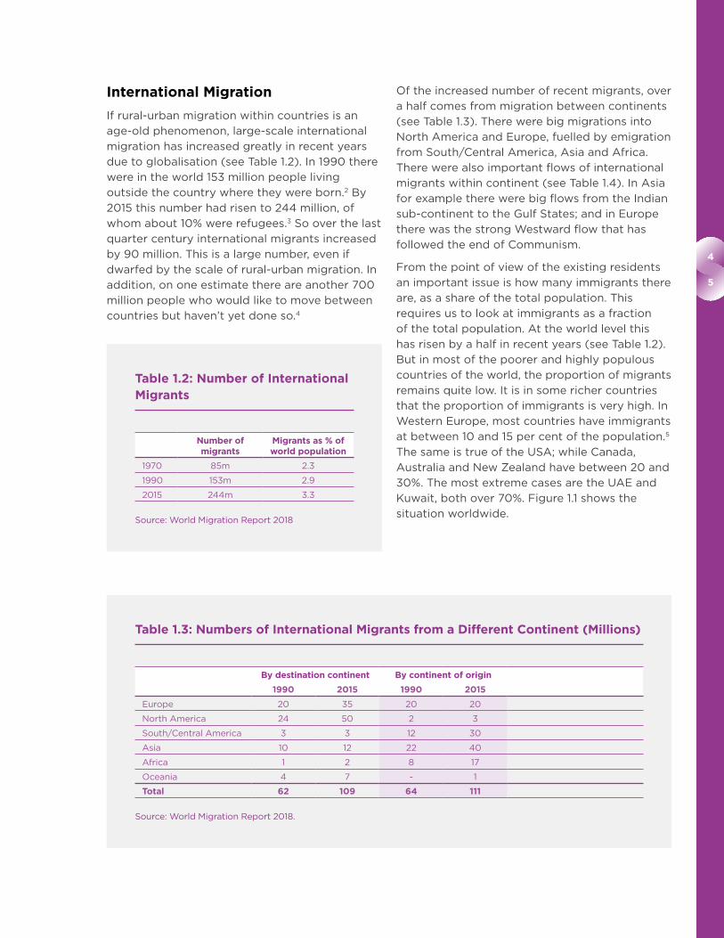
If rural-urban migration within countries is an
age-old phenomenon, large-scale international
migration has increased greatly in recent years
due to globalisation (see Table 1.2). In 1990 there
were in the world 153 million people living
outside the country where they were born.2 By
2015 this number had risen to 244 million, of
whom about 10% were refugees.3 So over the last
quarter century international migrants increased
by 90 million. This is a large number, even if
dwarfed by the scale of rural-urban migration. In
addition, on one estimate there are another 700
million people who would like to move between
countries but haven’t yet done so.4
Of the increased number of recent migrants, over
a half comes from migration between continents
(see Table 1.3). There were big migrations into
North America and Europe, fuelled by emigration
from South/Central America, Asia and Africa.
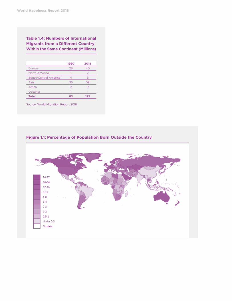
There were also important flows of international
migrants within continent (see Table 1.4). In Asia
for example there were big flows from the Indian
sub-continent to the Gulf States; and in Europe
there was the strong Westward flow that has
followed the end of Communism.
From the point of view of the existing residents
an important issue is how many immigrants there
are, as a share of the total population. This
requires us to look at immigrants as a fraction
of the total population. At the world level this
has risen by a half in recent years (see Table 1.2).
But in most of the poorer and highly populous
countries of the world, the proportion of migrants
remains quite low. It is in some richer countries
that the proportion of immigrants is very high. In
Western Europe, most countries have immigrants
at between 10 and 15 per cent of the population.5
The same is true of the USA; while Canada,
Australia and New Zealand have between 20 and
30%. The most extreme cases are the UAE and
Kuwait, both over 70%. Figure 1.1 shows the
situation worldwide.
Table 1.2: Number of International Migrants
Number of migrants
Migrants as % of world population
1970 85m 2.3
1990 153m 2.9
2015 244m 3.3
Source: World Migration Report 2018
Table 1.3: Numbers of International Migrants from a Different Continent (Millions)
By destination continent By continent of origin
1990 2015 1990 2015
Europe 20 35 20 20
North America 24 50 2 3
South/Central America 3 3 12 30
Asia 10 12 22 40
Africa 1 2 8 17
Oceania 4 7 - 1
Total 62 109 64 111
Source: World Migration Report 2018.
World Happiness Report 2018
Table 1.4: Numbers of International Migrants from a Different Country Within the Same Continent (Millions)
1990 2015
Europe 28 40
North America 1 2
South/Central America 4 6
Asia 36 59
Africa 13 17
Oceania 1 1
Total 83 125
Source: World Migration Report 2018
Figure 1.1: Percentage of Population Born Outside the Country

6
7
The Happiness of International Migrants
As already noted, migration within and between
countries has in general shifted people from less
to more productive work, and from lower to
higher incomes. In many cases the differences
have been quite extreme. International migration
has also saved many people from extremes of
oppression and physical danger – some 10%
of all international migrants are refugees, or
25 million people in total.
But what can be said about the happiness of
international migrants after they have reached
their destination? Chapter 2 of this report begins
with its usual ranking and analysis of the levels
and changes in the happiness of all residents,
whether locally born or immigrants, based on
samples of 1,000 per year, averaged for 2015-2017,
for 156 countries surveyed by the Gallup World
Poll. The focus is then switched to international
migration, separating out immigrants to permit
ranking of the average life evaluations of
immigrants for the 117 countries having more
than 100 foreign-born respondents between
2005 and 2017. (These foreign-born residents
may include short-term guest workers, longer
term immigrants, and serial migrants who shift
their residency more often, at different stages
of their upbringing, careers, and later lives).
So what determines the happiness of immigrants
living in different countries and coming from
different, other countries? Three striking facts
emerge.
1. In the typical country, immigrants are
about as happy as people born locally.
(The difference is under 0.1 point out of 10).
This is shown in Figure 1.2. However the figure
also shows that in the happiest countries
immigrants are significantly less happy than
locals, while the reverse is true in the least
happy countries. This is because of the
second finding.
2. The happiness of each migrant depends
not only on the happiness of locals (with a
weight of roughly 0.75) but also on the level
of happiness in the migrant’s country of
origin (with a weight of roughly 0.25). Thus
if a migrant goes (like many migrants) from
a less happy to a more happy country, the
migrant ends up somewhat less happy than
the locals. But the reverse is true if a migrant
goes from a more to a less happy country.
This explains the pattern shown in Figure 1.2
– and is a general (approximate) truth about
all bilateral flows. Another way of describing
this result is to say that on average, a migrant
gains in happiness about three-quarters of
the difference in average happiness between
the country of origin and the destination
country.
3. The happiness of immigrants also depends
importantly on how accepting the locals are
towards immigrants. (To measure acceptance
local residents were asked whether the
following were “good things” or “bad things”:
having immigrants in the country, having an
immigrant as a neighbour, and having an
immigrant marry your close relative). In a
country that was more accepting (by one
standard deviation) immigrants were happier
by 0.1 points (on a 0 to 10 scale).
Thus the analysis in Chapter 2 argues that
migrants gain on average if they move from
a less happy to a more happy country (which
is the main direction of migration). But that
argument was based on a simple comparison
Figure 1.2: Average Life Evaluation of Foreign-Born and Locally-Born Adults: by Country
Source: Chapter 2
World Happiness Report 2018
of the happiness of migrants with people in the
countries they have left. What if the migrants
were different types of people from those left
behind? Does this change the conclusion? As
Chapter 3 shows, the answer is, No. In Chapter 3
the happiness of migrants is compared with
individuals in their country of origin who are as
closely matched to the migrants as possible and
are thinking of moving. This again uses the data
from the Gallup World Poll. The results from
comparing the migrants with their look-a-likes
who stayed at home suggests that the average
international migrant gained 0.47 points (out of
10) in happiness by migration (as measured by
the Cantril ladder). This is a substantial gain.
But there is an important caveat: the majority
gain, but many lose. For example, in the only
controlled experiment that we know of, Tongans
applying to migrate to New Zealand were selected
on randomised basis.6 After moving, those who
had been selected to move were on average less
happy than those who (forcibly) stayed behind.
Migration clearly has its risks. These include
separation from loved ones, discrimination in the
new location, and a feeling of relative deprivation,
because you now compare yourself with others
who are richer than your previous reference
group back home.
One obvious question is: Do migrants become
happier or less happy the longer they have been
in a country? The answer is on average, neither
– their happiness remains flat. And in some
countries (where this has been studied) there is
evidence that second-generation migrants are no
happier than their immigrant parents.7 One way
of explaining these findings (which is developed
further in Chapter 4) is in terms of reference
groups: When people first move to a happier
country, their reference group is still largely their
country of origin. They experience an immediate
gain in happiness. As time passes, their objective
situation improves (which makes them still
happier) but their reference group becomes
increasingly the destination country (which
makes them less happy). These two effects
roughly offset each other. This process continues
in the second generation.
The Gallup World Poll excludes many current
refugees, since refugee camps are not surveyed.
Only in Germany is there sufficient evidence on
refugees, and in Germany refugees are 0.4 points
less happy than other migrants. But before they
moved, the refugees were also much less happy
than the other migrants were before they moved.
So refugees too are likely to have benefitted
from migration.
Thus average international migration benefits the
majority of migrants, but not all. Does the same
finding hold for the vast of the army of people
who have moved from the country to the towns
within less developed countries?
The Happiness of Rural-Urban Migrants
The fullest evidence on this comes from China and
is presented in Chapter 4. That chapter compares
the happiness of three groups of people:
• rural dwellers, who remain in the country,
• rural-urban migrants, now living in towns, and
• urban dwellers, who always lived in towns.
Migrants have roughly doubled their work
income by moving from the countryside, but
they are less happy than the people still living
in rural areas. Chapter 4 therefore goes on to
consider possible reasons for this. Could it be
that many of the migrants suffer because of the
remittances they send home? The evidence says,
No. Could it be that the people who migrate were
intrinsically less happy? The evidence says, No.
Could it be that urban life is more insecure than
life in the countryside – and involves fewer
friends and more discrimination? Perhaps.
The biggest factor affecting the happiness
of migrants is a change of reference group: the
happiness equation for migrants is similar to that
of urban dwellers, and different from that of rural
dwellers. This could explain why migrants say
they are happier as a result of moving – they
would no longer appreciate the simple pleasures
of rural life.
Human psychology is complicated, and be-
havioural economics has now documented
hundreds of ways in which people mispredict the
impact of decisions upon their happiness. It does
not follow that we should over-regulate their
lives, which would also cause unhappiness. It
does follow that we should protect people after
they make their decisions, by ensuring that
they can make positive social connections in
their new communities (hence avoiding or
reducing discrimination), and that they are
8
9
helped to fulfil the dreams that led them to
move in the first place.
It is unfortunate that there are not more studies
of rural-urban migration in other countries. In
Thailand one study finds an increase in happiness
among migrants8, while in South Africa one study
finds a decrease9.
The Happiness of Families Left Behind
In any case the migrants are not the only people
who matter. What about the happiness of the
families left behind? They frequently receive
remittances (altogether some $500 billion into
2015).10 But they lose the company and direct
support of the migrant. For international migrants,
we are able to examine this question in Chapter 3.
This is done by studying people in the country
of origin and examining the effect of having a
relative who is living abroad. On average this
experience increases both life-satisfaction and
positive affect. But there is also a rise in negative
affect (sadness, worry, anger), especially if
the migrant is abroad on temporary work.
Unfortunately, there is no comparable analysis of
families left behind by rural-urban migrants who
move to towns and cities in the same country.
The Happiness of the Original Residents in the Host Country
The final issue is how the arrival of migrants
affects the existing residents in the host country
or city. This is one of the most difficult issues in
all social science.
One approach is simply to explain happiness in
different countries by a whole host of variables
including the ratio of immigrants to the locally-
born population (the “immigrant share”). This is
done in Chapter 2 and shows no effect of the
immigrant share on the average happiness of
the locally born.11 It does however show that the
locally born population (like immigrants) are
happier, other things equal, if the country is
more accepting of immigrants.12
Nevertheless, we know that immigration can
create tensions, as shown by its high political
salience in many immigrant-receiving countries,
especially those on migration trails from unhappy
source countries to hoped-for havens in the north.
Several factors contribute to explaining whether
migration is welcomed by the local populations.13
First, scale is important. Moderate levels of
immigration cause fewer problems than rapid
surges.14 Second, the impact of unskilled
immigration falls mainly on unskilled people in
the host country, though the impact on public
services is often exaggerated and the positive
contribution of immigrants is often underestimated.
Third, the degree of social distress caused to the
existing residents depends importantly on their
own frame of mind – a more open-minded
attitude is better both for immigrants and for
the original residents. Fourth, the attitude of
immigrants is also important – if they are to find
and accept opportunities to connect with the
local populations, this is better for everyone.
Even if such integration may initially seem
difficult, in the long run it has better results –
familiarity eventually breeds acceptance,15 and
inter-marriage more than anything blurs the
differences. The importance of attitudes is
documented in the Gallup Annex on migrant
acceptance, and in Chapter 2, where the migrant
acceptance index is shown to increase the
happiness of both sectors of the population –
immigrants and the locally born.
Chapter 5 completes the set of migration chapters.
It seeks to explain why so many people emigrate
from Latin American countries, and also to
assess the happiness consequences for those
who do migrate. In Latin America, as elsewhere,
those who plan to emigrate are on average less
happy than others similar to themselves in
income, gender and age. They are also on average
wealthier – in other words they are “frustrated
achievers”. But those who do emigrate from Latin
American countries also gain less in happiness
than emigrants from some other continents. This
is because, as shown in chapters 2 and 6, they
come from pretty happy countries. Their choice
of destination countries is also a less happy mix.
This combination lessens their average gains,
because of the convergence of immigrant
happiness to the general happiness levels in the
countries to which they move, as documented in
Chapter 2. If immigrants from Latin America are
compared to other migrants to the same countries,
they do very well in relation both to other
immigrants and to the local population. This is
shown in Chapter 2 for immigration to Canada
and the United Kingdom – countries with large

World Happiness Report 2018
enough happiness surveys to permit comparison
of the happiness levels of immigrants from up to
100 different source countries.
Chapter 6 completes the Latin American special
package by seeking to explain the happiness
bulge in Latin America. Life satisfaction in Latin
America is substantially higher than would be
predicted based on income, corruption, and
other standard variables, including having
someone to count on. Even more remarkable are
the levels of positive affect, with eight of the
world’s top ten countries being found in Latin
America. To explain these differences, Chapter 6
convincingly demonstrates the strength of family
relationships in Latin America. In a nutshell, the
source of the extra Latin American happiness lies
in the remarkable warmth and strength of family
bonds, coupled with the greater importance that
Latin Americans attach to social life in general,
and especially to the family. They are more
satisfied with their family life and, more than
elsewhere, say that one of their main goals is
making their parents proud.
Conclusion
In conclusion, there are large gaps in happiness
between countries, and these will continue to
create major pressures to migrate. Some of those
who migrate between countries will benefit and
others will lose. In general, those who move to
happier countries than their own will gain in
happiness, while those who move to unhappier
countries will tend to lose. Those left behind will
not on average lose, although once again there
will be gainers and losers. Immigration will
continue to pose both opportunities and costs
for those who move, for those who remain
behind, and for natives of the immigrant-
receiving countries.
Where immigrants are welcome and where they
integrate well, immigration works best. A more
tolerant attitude in the host country will prove
best for migrants and for the original residents.
But there are clearly limits to the annual flows
which can be accommodated without damage to
the social fabric that provides the very basis of
the country’s attraction to immigrants. One
obvious solution, which has no upper limit, is to
raise the happiness of people in the sending
countries – perhaps by the traditional means of
foreign aid and better access to rich-country
markets, but more importantly by helping them
to grow their own levels of trust, and institutions
of the sort that make possible better lives in the
happier countries.

10
11
To re-cap, the structure of the chapters that
follow is:
Chapter 2 analyses the happiness of the total
population in each country, the happiness of the
immigrants there, and also the happiness of
those born locally.
Chapter 3 estimates how international migrants
have improved (or reduced) their happiness by
moving, and how their move has affected the
families left behind.
Chapter 4 analyses how rural-urban migration
within a country (here China) affects the happiness
of the migrants.
Chapter 5 looks at Latin America and analyses
the causes and consequences of emigration.
Chapter 6 explains why people in Latin American
countries are on average, other things equal,
unusually happy.
In addition,
Chapter 7 uses US data set in a global context to
describe some growing health risks created by
human behaviour, especially obesity, substance
abuse, and depression.

World Happiness Report 2018
Endnotes
1 As Chapter 4 documents, in 2015 the number of rural hukou residents in towns was 225 million.
2 This is based on the definitions given in the sources to UN-DESA (2015) most of which are “foreign born”.
3 See IOM (2017).
4 See Esipova, N., Ray, J. and Pugliese, A. (2017).
5 See World Migration Report 2018, Chapter 3.
6 See Chapter 3.
7 See Safi, M. (2009).
8 De Jong et al. (2002)
9 Mulcahy & Kollamparambil (2016)
10 Ratha et al. (2016)
11 In this analysis, the equation includes all the standard explanatory variables as well, making it possible to identify the causal effect of the immigrant share. (This share also of course depends on the happiness level of the country but in a much different equation). A similar approach, using individual data, is used by Akay et al (2014) comparing across German regions, and by Betz and Simpson (2013) across the countries covered by the European Social Survey. Both found effects that were positive (for only some regions in Akay et al (2014) but quantitatively tiny. Our results do not rule out the possibility of small effects of either sign.
12 One standard deviation raises their happiness on average by 0.15 points. This estimate comes from an equation including, also on the right-hand side, all the standard variables explaining country-happiness used in Chapter 2. This provides identification of an effect running from acceptance to happiness rather than vice versa.
13 See Putnam, R. D. (2007).
14 Another important factor is the availability of sparsely- populated space. Earlier migrations into North America and Oceania benefitted from more of this.
15 See for example Rao (2018).
References
Akay, A., et al. (2014). The impact of immigration on the well-being of natives. Journal of Economic Behavior & Organization, 103(C), 72-92.
Betz, W., & Simpson, N. (2013). The effects of international migration on the well-being of native populations in Europe. IZA Journal of Migration, 2(1), 1-21.
De Jong, G. F., et al. (2002). For Better, For Worse: Life Satisfaction Consequences of Migration. International Migration Review, 36(3), 838-863. doi: 10.1111/j.1747-7379.2002.tb00106.x
Esipova, N., Ray, J. and Pugliese, A. (2017) Number of potential migrants worldwide tops 700 million. Retrieved February 28, 2018 from http://news.gallup.com/poll/211883/number-potential-migrants-worldwide-tops-700-million.aspx?g_source=link_NEWSV9&g_medium=TOPIC&g_ campaign=item_&g_content=Number%2520of%2520Potential %2520Migrants%2520Worldwide%2520 Tops%2520700%-2520Million
IOM (2017), World Migration Report 2018, UN, New York.
Mulcahy, K., & Kollamparambil, U. (2016). The Impact of Rural-Urban Migration on Subjective Well-Being in South Africa. The Journal of Development Studies, 52(9), 1357-1371. doi: 10.1080/00220388.2016.1171844
Putnam, R. D. (2007). E Pluribus Unum: Diversity and Commu-nity in the Twenty-first Century The 2006 Johan Skytte Prize Lecture. Scandinavian Political Studies, 30(2), 137-174. doi: 10.1111/j.1467-9477.2007.00176.x
Rao, G. (2018). Familiarity Does Not Breed Contempt: Diversity, Discrimination and Generosity in Delhi Schools.
Ratha, D., et al. (2016). Migration and remittances Factbook 2016: World Bank Publications.
Safi, M. (2009). Immigrants’ life satisfaction in Europe: Between assimilation and discrimination. European Sociological Review, 26(2), 159-176.
UN-DESA. (2015). International Migrant Stock: The 2015 Revision. Retrieved from: www.un.org/en/development/desa/population/migration/data/estimates2/index.shtml
12
13Chapter 2
International Migration and World Happiness
John F. Helliwell, Canadian Institute for Advanced Research and Vancouver School of Economics, University of British Columbia
Haifang Huang, Associate Professor, Department of Economics, University of Alberta
Shun Wang, Associate Professor, KDI School of Public Policy and Management
Hugh Shiplett, Vancouver School of Economics, University of British Columbia
The authors are grateful to the Canadian Institute for Advanced Research, the KDI School, and the Ernesto Illy Foundation for research support, and to the UK Office for National Statistics and Gallup for data access and assistance. The authors are also grateful for helpful advice and comments from Claire Bulger, Jan-Emmanuel De Neve, Neli Esposito, Carol Graham, Jon Hall, Martijn Hendricks, Richard Layard, Max Norton, Julie Ray, Mariano Rojas, and Meik Wiking.

World Happiness Report 2018
Introduction
This is the sixth World Happiness Report. Its
central purpose remains just what it was in the
first Report in April 2012, to survey the science
of measuring and understanding subjective
well-being. In addition to presenting updated
rankings and analysis of life evaluations through-
out the world, each World Happiness Report has
had a variety of topic chapters, often dealing
with an underlying theme for the report as a
whole. For the World Happiness Report 2018 our
special focus is on migration. Chapter 1 sets
global migration in broad context, while in this
chapter we shall concentrate on life evaluations
of the foreign-born populations of each country
where the available samples are large enough to
provide reasonable estimates. We will compare
these levels with those of respondents who were
born in the country where they were surveyed.
Chapter 3 will then examine the evidence on
specific migration flows, assessing the likely
happiness consequences (as represented both
by life evaluations and measures of positive
and negative affect) for international migrants
and those left behind in their birth countries.
Chapter 4 considers internal migration in more
detail, concentrating on the Chinese experience,
by far the largest example of migration from the
countryside to the city. Chapter 5 completes our
migration package with special attention to Latin
American migration.
Before presenting our evidence and rankings of
immigrant happiness, we first present, as usual,
the global and regional population-weighted
distributions of life evaluations using the average
for surveys conducted in the three years 2015-2017.
This is followed by our rankings of national
average life evaluations, again based on data
from 2015-2017, and then an analysis of changes
in life evaluations, once again for the entire
resident populations of each country, from
2008-2010 to 2015-2017.
Our rankings of national average life evaluations
will be accompanied by our latest attempts to
show how six key variables contribute to explaining
the full sample of national annual average scores
over the whole period 2005-2017. These variables
are GDP per capita, social support, healthy life
expectancy, social freedom, generosity, and
absence of corruption. Note that we do not
construct our happiness measure in each country
using these six factors – the scores are instead
based on individuals’ own assessments of their
subjective well-being. Rather, we use the variables
to explain the variation of happiness across
countries. We shall also show how measures of
experienced well-being, especially positive
emotions, supplement life circumstances in
explaining higher life evaluations.
Then we turn to the main focus, which is migration
and happiness. The principal results in this
chapter are for the life evaluations of the foreign-
born and domestically born populations of every
country where there is a sufficiently large
sample of the foreign-born to provide reasonable
estimates. So that we may consider a sufficiently
large number of countries, we do not use just the
2015-2017 data used for the main happiness
rankings, but instead use all survey available
since the start of the Gallup World Poll in 2005.
Life Evaluations Around the World
We first consider the population-weighted global
and regional distributions of individual life
evaluations, based on how respondents rate their
lives. In the rest of this chapter, the Cantril ladder
is the primary measure of life evaluations used,
and “happiness” and “subjective well-being” are
used interchangeably. All the global analysis on
the levels or changes of subjective well-being
refers only to life evaluations, specifically, the
Cantril ladder. But in several of the subsequent
chapters, parallel analysis will be done for
measures of positive and negative affect, thus
broadening the range of data used to assess
the consequences of migration.
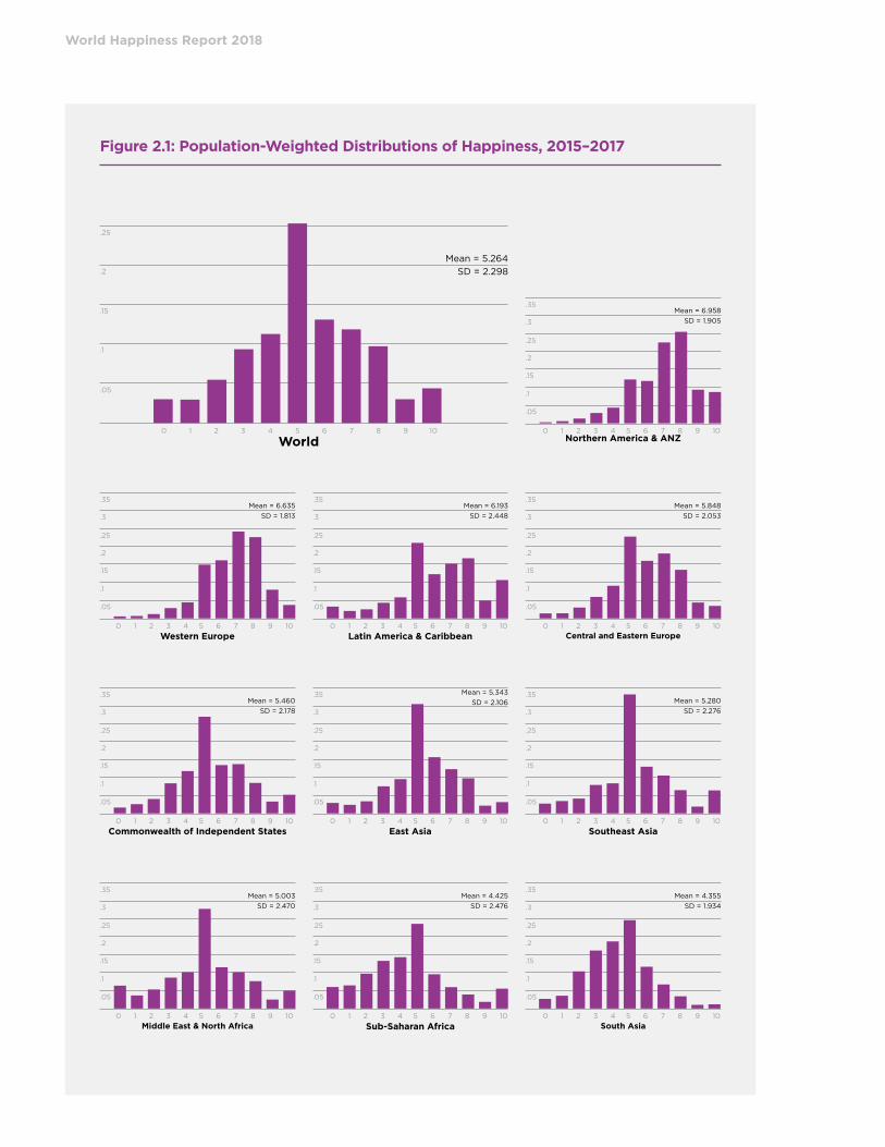
The various panels of Figure 2.1 contain bar
charts showing for the world as a whole, and for
each of 10 global regions,1 the distribution of the
2015-2017 answers to the Cantril ladder question
asking respondents to value their lives today on
a 0 to 10 scale, with the worst possible life as a 0
and the best possible life as a 10. It is important
to consider not just average happiness in a
community or country, but also how it is
distributed. Most studies of inequality have
focused on inequality in the distribution of
income and wealth,2 while in Chapter 2 of World
Happiness Report 2016 Update we argued that
just as income is too limited an indicator for the
overall quality of life, income inequality is too

14
15
limited a measure of overall inequality.3 For
example, inequalities in the distribution of
health care4 and education5 have effects on life
satisfaction above and beyond those flowing
through their effects on income. We showed
there, and have verified in fresh estimates for this
report,6 that the effects of happiness equality are
often larger and more systematic than those of
income inequality. Figure 2.1 shows that well-
being inequality is least in Western Europe,
Northern America and Oceania, and South Asia;
and greatest in Latin America, sub-Saharan
Africa, and the Middle East and North Africa.
In Table 2.1 we present our latest modeling of
national average life evaluations and measures of
positive and negative affect (emotion) by country
and year.7 For ease of comparison, the table has
the same basic structure as Table 2.1 in World
Happiness Report 2017. The major difference
comes from the inclusion of data for 2017,
thereby increasing by about 150 (or 12%) the
number of country-year observations. The resulting
changes to the estimated equation are very
slight.8 There are four equations in Table 2.1. The
first equation provides the basis for constructing
the sub-bars shown in Figure 2.2.
The results in the first column of Table 2.1 explain
national average life evaluations in terms of six key
variables: GDP per capita, social support, healthy
life expectancy, freedom to make life choices,
generosity, and freedom from corruption.9 Taken
together, these six variables explain almost
three-quarters of the variation in national annual
average ladder scores among countries, using
data from the years 2005 to 2017. The model’s
predictive power is little changed if the year
fixed effects in the model are removed, falling
from 74.2% to 73.5% in terms of the adjusted
R-squared.
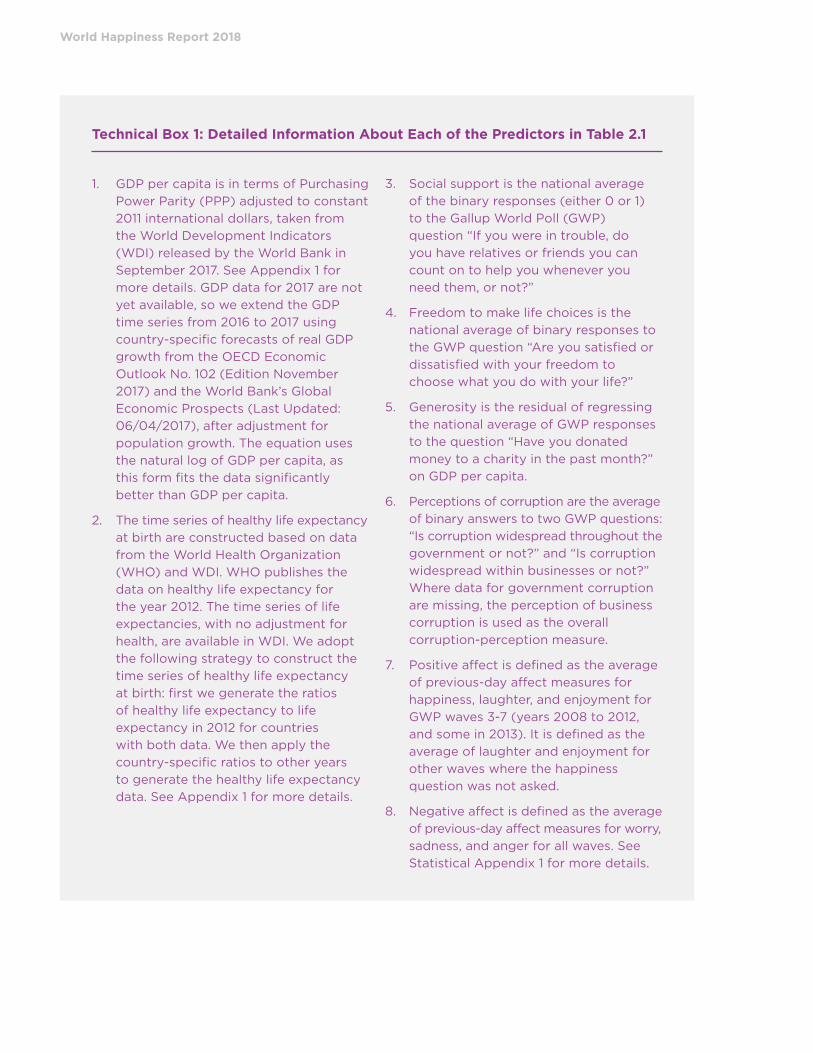
The second and third columns of Table 2.1 use
the same six variables to estimate equations
for national averages of positive and negative
affect, where both are based on answers about
yesterday’s emotional experiences (see Technical
Box 1 for how the affect measures are constructed).
In general, the emotional measures, and especially
negative emotions, are differently, and much less
fully, explained by the six variables than are life
evaluations. Per-capita income and healthy life
expectancy have significant effects on life
evaluations, but not, in these national average
data, on either positive or negative affect. The
situation changes when we consider social
variables. Bearing in mind that positive and
negative affect are measured on a 0 to 1 scale,
while life evaluations are on a 0 to 10 scale, social
support can be seen to have similar proportionate
effects on positive and negative emotions as on
life evaluations. Freedom and generosity have
even larger influences on positive affect than on
the ladder. Negative affect is significantly reduced
by social support, freedom, and absence of
corruption.
In the fourth column we re-estimate the life
evaluation equation from column 1, adding both
positive and negative affect to partially implement
the Aristotelian presumption that sustained
positive emotions are important supports for a
good life.10 The most striking feature is the extent to
which the results buttress a finding in psychology
that the existence of positive emotions matters
much more than the absence of negative ones.11
Positive affect has a large and highly significant
impact in the final equation of Table 2.1, while
negative affect has none.
As for the coefficients on the other variables in
the final equation, the changes are material only
on those variables – especially freedom and
generosity – that have the largest impacts on
positive affect. Thus we infer that positive
emotions play a strong role in support of life
evaluations, and that most of the impact of
freedom and generosity on life evaluations is
mediated by their influence on positive emotions.
That is, freedom and generosity have large
impacts on positive affect, which in turn has a
major impact on life evaluations. The Gallup
World Poll does not have a widely available
measure of life purpose to test whether it too
would play a strong role in support of high life
evaluations. However, newly available data from
the large samples of UK data does suggest that
life purpose plays a strongly supportive role,
independent of the roles of life circumstances
and positive emotions.
World Happiness Report 2018
Figure 2.1: Population-Weighted Distributions of Happiness, 2015–2017
.25
.15
.05
.2
.1
Mean = 5.264
SD = 2.298
World
.25
.1
.05
.3
.15
.35
.2
Mean = 6.958
SD = 1.905
Northern America & ANZ
.25
.1
.05
.3
.15
.35
.2
Mean = 5.848
SD = 2.053
Central and Eastern Europe
.25
.1
.05
.3
.15
.35
.2
Mean = 6.193
SD = 2.448
Latin America & Caribbean
.25
.1
.05
.3
.15
.35
.2
Mean = 6.635
SD = 1.813
Western Europe
.25
.1
.05
.3
.15
.35
.2
Mean = 5.280
SD = 2.276
Southeast Asia
.25
.1
.05
.3
.15
.35
.2
Mean = 5.343
SD = 2.106
East Asia
.25
.1
.05
.3
.15
.35
.2
Mean = 5.460
SD = 2.178
Commonwealth of Independent States
.25
.1
.05
.3
.15
.35
.2
Mean = 4.355
SD = 1.934
South Asia
.25
.1
.05
.3
.15
.35
.2
Mean = 4.425
SD = 2.476
Sub-Saharan Africa
.25
.1
.05
.3
.15
.35
.2
Mean = 5.003
SD = 2.470
Middle East & North Africa
0 1 2 3 4 5 6 7 8 9 10
0 1 2 3 4 5 6 7 8 9 10
0 1 2 3 4 5 6 7 8 9 100 1 2 3 4 5 6 7 8 9 10
0 1 2 3 4 5 6 7 8 9 10
0 1 2 3 4 5 6 7 8 9 10
0 1 2 3 4 5 6 7 8 9 10
0 1 2 3 4 5 6 7 8 9 10
0 1 2 3 4 5 6 7 8 9 10
0 1 2 3 4 5 6 7 8 9 10
0 1 2 3 4 5 6 7 8 9 10

16
17
Table 2.1: Regressions to Explain Average Happiness Across Countries (Pooled OLS)
Dependent Variable
Independent Variable Cantril Ladder Positive Affect Negative Affect Cantril Ladder
Log GDP per capita 0.311 -.003 0.011 0.316
(0.064)*** (0.009) (0.009) (0.063)***
Social support 2.447 0.26 -.289 1.933
(0.39)*** (0.049)*** (0.051)*** (0.395)***
Healthy life expectancy at birth 0.032 0.0002 0.001 0.031
(0.009)*** (0.001) (0.001) (0.009)***
Freedom to make life choices 1.189 0.343 -.071 0.451
(0.302)*** (0.038)*** (0.042)* (0.29)
Generosity 0.644 0.145 0.001 0.323
(0.274)** (0.03)*** (0.028) (0.272)
Perceptions of corruption -.542 0.03 0.098 -.626
(0.284)* (0.027) (0.025)*** (0.271)**
Positive affect 2.211
(0.396)***
Negative affect 0.204
(0.442)
Year fixed effects Included Included Included Included
Number of countries 157 157 157 157
Number of obs. 1394 1391 1393 1390
Adjusted R-squared 0.742 0.48 0.251 0.764
Notes: This is a pooled OLS regression for a tattered panel explaining annual national average Cantril ladder responses from all available surveys from 2005 to 2017. See Technical Box 1 for detailed information about each of the predictors. Coefficients are reported with robust standard errors clustered by country in parentheses. ***, **, and * indicate significance at the 1, 5 and 10 percent levels respectively.
World Happiness Report 2018
Technical Box 1: Detailed Information About Each of the Predictors in Table 2.1
1. GDP per capita is in terms of Purchasing
Power Parity (PPP) adjusted to constant
2011 international dollars, taken from
the World Development Indicators
(WDI) released by the World Bank in
September 2017. See Appendix 1 for
more details. GDP data for 2017 are not
yet available, so we extend the GDP
time series from 2016 to 2017 using
country-specific forecasts of real GDP
growth from the OECD Economic
Outlook No. 102 (Edition November
2017) and the World Bank’s Global
Economic Prospects (Last Updated:
06/04/2017), after adjustment for
population growth. The equation uses
the natural log of GDP per capita, as
this form fits the data significantly
better than GDP per capita.
2. The time series of healthy life expectancy
at birth are constructed based on data
from the World Health Organization
(WHO) and WDI. WHO publishes the
data on healthy life expectancy for
the year 2012. The time series of life
expectancies, with no adjustment for
health, are available in WDI. We adopt
the following strategy to construct the
time series of healthy life expectancy
at birth: first we generate the ratios
of healthy life expectancy to life
expectancy in 2012 for countries
with both data. We then apply the
country-specific ratios to other years
to generate the healthy life expectancy
data. See Appendix 1 for more details.
3. Social support is the national average
of the binary responses (either 0 or 1)
to the Gallup World Poll (GWP)
question “If you were in trouble, do
you have relatives or friends you can
count on to help you whenever you
need them, or not?”
4. Freedom to make life choices is the
national average of binary responses to
the GWP question “Are you satisfied or
dissatisfied with your freedom to
choose what you do with your life?”
5. Generosity is the residual of regressing
the national average of GWP responses
to the question “Have you donated
money to a charity in the past month?”
on GDP per capita.
6. Perceptions of corruption are the average
of binary answers to two GWP questions:
“Is corruption widespread throughout the
government or not?” and “Is corruption
widespread within businesses or not?”
Where data for government corruption
are missing, the perception of business
corruption is used as the overall
corruption-perception measure.
7. Positive affect is defined as the average
of previous-day affect measures for
happiness, laughter, and enjoyment for
GWP waves 3-7 (years 2008 to 2012,
and some in 2013). It is defined as the
average of laughter and enjoyment for
other waves where the happiness
question was not asked.
8. Negative affect is defined as the average
of previous-day affect measures for worry,
sadness, and anger for all waves. See
Statistical Appendix 1 for more details.
18
19
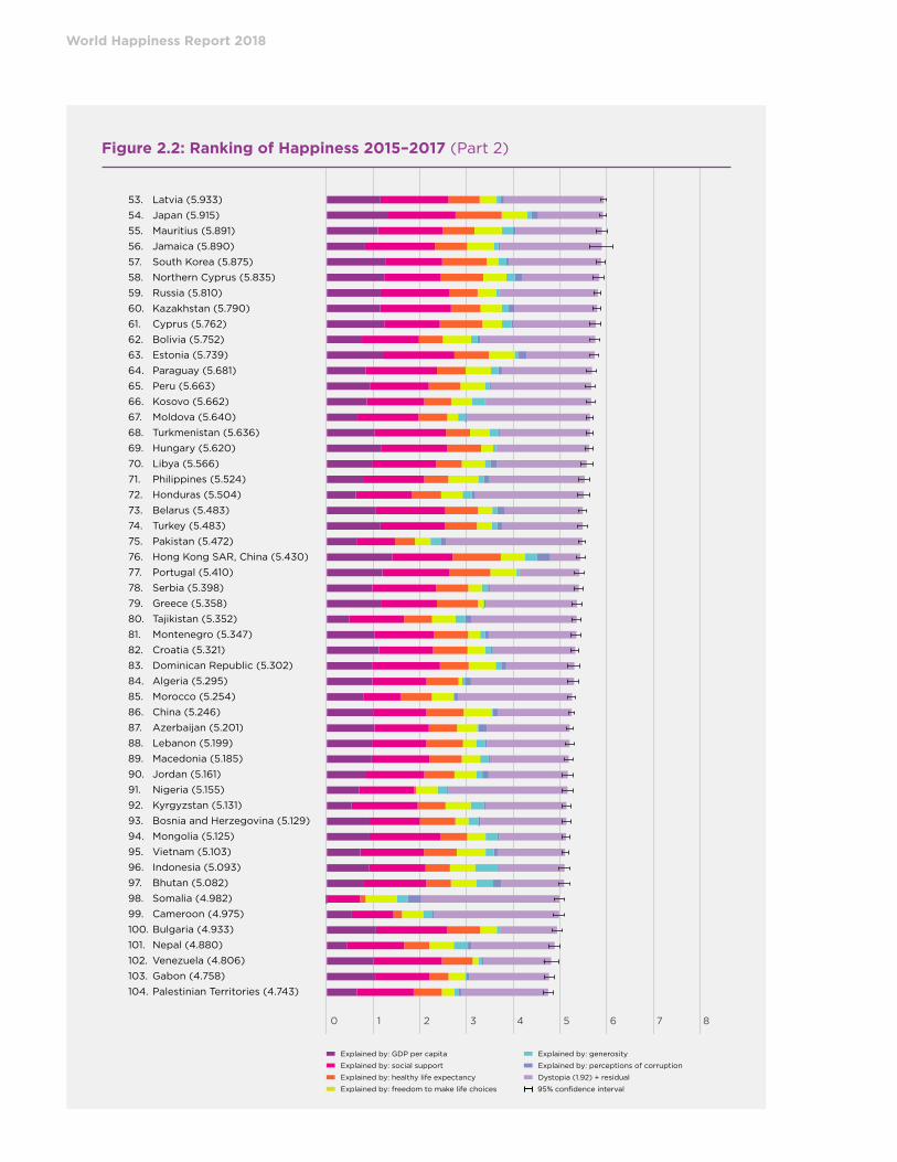
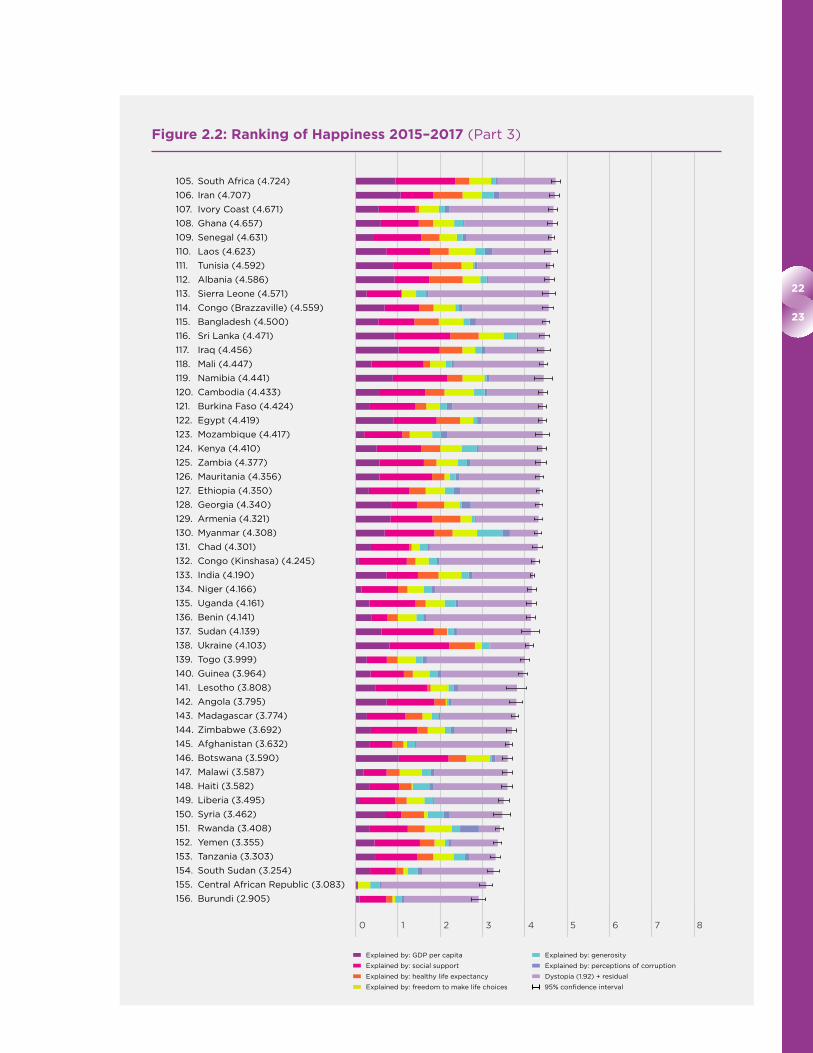
Ranking of Happiness by Country
Figure 2.2 (below) shows the average ladder
score (the average answer to the Cantril ladder
question, asking people to evaluate the quality of
their current lives on a scale of 0 to 10) for each
country, averaged over the years 2015-2017. Not
every country has surveys in every year; the total
sample sizes are reported in the statistical
appendix, and are reflected in Figure 2.2 by the
horizontal lines showing the 95% confidence
regions. The confidence regions are tighter for
countries with larger samples. To increase the
number of countries ranked, we also include four
that had no 2015-2017 surveys, but did have one
in 2014. This brings the number of countries
shown in Figure 2.2 to 156.
The overall length of each country bar represents
the average ladder score, which is also shown in
numerals. The rankings in Figure 2.2 depend only
on the average Cantril ladder scores reported by
the respondents.
Each of these bars is divided into seven
segments, showing our research efforts to find
possible sources for the ladder levels. The first
six sub-bars show how much each of the six
key variables is calculated to contribute to that
country’s ladder score, relative to that in a
hypothetical country called Dystopia, so named
because it has values equal to the world’s lowest
national averages for 2015-2017 for each of the six
key variables used in Table 2.1. We use Dystopia as
a benchmark against which to compare each
other country’s performance in terms of each of
the six factors. This choice of benchmark permits
every real country to have a non-negative
contribution from each of the six factors. We
calculate, based on the estimates in the first
column of Table 2.1, that Dystopia had a 2015-
2017 ladder score equal to 1.92 on the 0 to 10
scale. The final sub-bar is the sum of two
components: the calculated average 2015-2017
life evaluation in Dystopia (=1.92) and each
country’s own prediction error, which measures
the extent to which life evaluations are higher or
lower than predicted by our equation in the first
column of Table 2.1. These residuals are as likely
to be negative as positive.12
It might help to show in more detail how we
calculate each factor’s contribution to average
life evaluations. Taking the example of healthy life
expectancy, the sub-bar in the case of Tanzania
is equal to the number of years by which healthy
life expectancy in Tanzania exceeds the world’s
lowest value, multiplied by the Table 2.1 coefficient
for the influence of healthy life expectancy on
life evaluations. The width of these different
sub-bars then shows, country-by-country, how
much each of the six variables is estimated to
contribute to explaining the international ladder
differences. These calculations are illustrative
rather than conclusive, for several reasons. First,
the selection of candidate variables is restricted
by what is available for all these countries.
Traditional variables like GDP per capita and
healthy life expectancy are widely available. But
measures of the quality of the social context,
which have been shown in experiments and
national surveys to have strong links to life
evaluations and emotions, have not been
sufficiently surveyed in the Gallup or other
global polls, or otherwise measured in statistics
available for all countries. Even with this limited
choice, we find that four variables covering
different aspects of the social and institutional
context – having someone to count on, generosity,
freedom to make life choices and absence of
corruption – are together responsible for more
than half of the average difference between each
country’s predicted ladder score and that in
Dystopia in the 2015-2017 period. As shown in
Table 19 of Statistical Appendix 1, the average
country has a 2015-2017 ladder score that is 3.45
points above the Dystopia ladder score of 1.92.
Of the 3.45 points, the largest single part (35%)
comes from social support, followed by GDP per
capita (26%) and healthy life expectancy (17%),
and then freedom (13%), generosity (5%), and
corruption (3%).13
Our limited choice means that the variables we
use may be taking credit properly due to other
better variables, or to other unmeasured factors.
There are also likely to be vicious or virtuous
circles, with two-way linkages among the variables.
For example, there is much evidence that those
who have happier lives are likely to live longer,
be more trusting, be more cooperative, and be
generally better able to meet life’s demands.14
This will feed back to improve health, GDP,
generosity, corruption, and sense of freedom.
Finally, some of the variables are derived from
the same respondents as the life evaluations and
hence possibly determined by common factors.
This risk is less using national averages, because

World Happiness Report 2018
individual differences in personality and many
life circumstances tend to average out at the
national level.
To provide more assurance that our results are
not seriously biased because we are using the
same respondents to report life evaluations,
social support, freedom, generosity, and
corruption, we tested the robustness of our
procedure (see Statistical Appendix 1 for more
detail) by splitting each country’s respondents
randomly into two groups, and using the average
values for one group for social support, freedom,
generosity, and absence of corruption in the
equations to explain average life evaluations in
the other half of the sample. The coefficients on
each of the four variables fall, just as we would
expect. But the changes are reassuringly small
(ranging from 1% to 5%) and are far from being
statistically significant.15
The seventh and final segment is the sum of
two components. The first component is a fixed
number representing our calculation of the
2015-2017 ladder score for Dystopia (=1.92). The
second component is the 2015-2017 residual for
each country. The sum of these two components
comprises the right-hand sub-bar for each
country; it varies from one country to the next
because some countries have life evaluations
above their predicted values, and others lower.
The residual simply represents that part of
the national average ladder score that is not
explained by our model; with the residual
included, the sum of all the sub-bars adds up
to the actual average life evaluations on which
the rankings are based.
What do the latest data show for the 2015-2017
country rankings? Two features carry over from
previous editions of the World Happiness Report.
First, there is a lot of year-to-year consistency in
the way people rate their lives in different countries.
Thus there remains a four-point gap between the
10 top-ranked and the 10 bottom-ranked countries.
The top 10 countries in Figure 2.2 are the same
countries that were top-ranked in World Happiness
Report 2017, although there has been some
swapping of places, as is to be expected among
countries so closely grouped in average scores.
The top five countries are the same ones that
held the top five positions in World Happiness
Report 2017, but Finland has vaulted from
5th place to the top of the rankings this year.
Although four places may seem a big jump, all
the top five countries last year were within the
same statistical confidence band, as they are
again this year. Norway is now in 2nd place,
followed by Denmark, Iceland and Switzerland in
3rd, 4th and 5th places. The Netherlands, Canada
and New Zealand are 6th, 7th and 8th, just as
they were last year, while Australia and Sweden
have swapped positions since last year, with
Sweden now in 9th and Australia in 10th position.
In Figure 2.2, the average ladder score differs
only by 0.15 between the 1st and 5th position,
and another 0.21 between 5th and 10th positions.
Compared to the top 10 countries in the current
ranking, there is a much bigger range of scores
covered by the bottom 10 countries. Within this
group, average scores differ by as much as 0.7
points, more than one-fifth of the average
national score in the group. Tanzania, Rwanda
and Botswana have anomalous scores, in the
sense that their predicted values based on their
performance on the six key variables, would
suggest they would rank much higher than
shown by the survey answers.
Despite the general consistency among the top
countries scores, there have been many significant
changes in the rest of the countries. Looking at
changes over the longer term, many countries
have exhibited substantial changes in average
scores, and hence in country rankings, between
2008-2010 and 2015-2017, as shown later in
more detail.
When looking at average ladder scores, it is also
important to note the horizontal whisker lines at
the right-hand end of the main bar for each
country. These lines denote the 95% confidence
regions for the estimates, so that countries with
overlapping error bars have scores that do not
significantly differ from each other. Thus, as already
noted, the five top-ranked countries (Finland,
Norway, Denmark, Iceland, and Switzerland) have
overlapping confidence regions, and all have
national average ladder scores either above or
just below 7.5.
Average life evaluations in the top 10 countries
are thus more than twice as high as in the bottom
10. If we use the first equation of Table 2.1 to look
for possible reasons for these very different life
evaluations, it suggests that of the 4.10 point
difference, 3.22 points can be traced to differences
in the six key factors: 1.06 points from the GDP

20
21
Figure 2.2: Ranking of Happiness 2015–2017 (Part 1)
1. Finland (7.632)
2. Norway (7.594)
3. Denmark (7.555)
4. Iceland (7.495)
5. Switzerland (7.487)
6. Netherlands (7.441)
7. Canada (7.328)
8. New Zealand (7.324)
9. Sweden (7.314)
10. Australia (7.272)
11. Israel (7.190)
12. Austria (7.139)
13. Costa Rica (7.072)
14. Ireland (6.977)
15. Germany (6.965)
16. Belgium (6.927)
17. Luxembourg (6.910)
18. United States (6.886)
19. United Kingdom (6.814)
20. United Arab Emirates (6.774)
21. Czech Republic (6.711)
22. Malta (6.627)
23. France (6.489)
24. Mexico (6.488)
25. Chile (6.476)
26. Taiwan Province of China (6.441)
27. Panama (6.430)
28. Brazil (6.419)
29. Argentina (6.388)
30. Guatemala (6.382)
31. Uruguay (6.379)
32. Qatar (6.374)
33. Saudi (Arabia (6.371)
34. Singapore (6.343)
35. Malaysia (6.322)
36. Spain (6.310)
37. Colombia (6.260)
38. Trinidad & Tobago (6.192)
39. Slovakia (6.173)
40. El Salvador (6.167)
41. Nicaragua (6.141)
42. Poland (6.123)
43. Bahrain (6.105)
44. Uzbekistan (6.096)
45. Kuwait (6.083)
46. Thailand (6.072)
47. Italy (6.000)
48. Ecuador (5.973)
49. Belize (5.956)
50. Lithuania (5.952)
51. Slovenia (5.948)
52. Romania (5.945)
0 1 2 3 4 5 6 7 8
Explained by: GDP per capita
Explained by: social support
Explained by: healthy life expectancy
Explained by: freedom to make life choices
Explained by: generosity
Explained by: perceptions of corruption
Dystopia (1.92) + residual
95% confidence interval
World Happiness Report 2018
Figure 2.2: Ranking of Happiness 2015–2017 (Part 2)
53. Latvia (5.933)
54. Japan (5.915)
55. Mauritius (5.891)
56. Jamaica (5.890)
57. South Korea (5.875)
58. Northern Cyprus (5.835)
59. Russia (5.810)
60. Kazakhstan (5.790)
61. Cyprus (5.762)
62. Bolivia (5.752)
63. Estonia (5.739)
64. Paraguay (5.681)
65. Peru (5.663)
66. Kosovo (5.662)
67. Moldova (5.640)
68. Turkmenistan (5.636)
69. Hungary (5.620)
70. Libya (5.566)
71. Philippines (5.524)
72. Honduras (5.504)
73. Belarus (5.483)
74. Turkey (5.483)
75. Pakistan (5.472)
76. Hong Kong SAR, China (5.430)
77. Portugal (5.410)
78. Serbia (5.398)
79. Greece (5.358)
80. Tajikistan (5.352)
81. Montenegro (5.347)
82. Croatia (5.321)
83. Dominican Republic (5.302)
84. Algeria (5.295)
85. Morocco (5.254)
86. China (5.246)
87. Azerbaijan (5.201)
88. Lebanon (5.199)
89. Macedonia (5.185)
90. Jordan (5.161)
91. Nigeria (5.155)
92. Kyrgyzstan (5.131)
93. Bosnia and Herzegovina (5.129)
94. Mongolia (5.125)
95. Vietnam (5.103)
96. Indonesia (5.093)
97. Bhutan (5.082)
98. Somalia (4.982)
99. Cameroon (4.975)
100. Bulgaria (4.933)
101. Nepal (4.880)
102. Venezuela (4.806)
103. Gabon (4.758)
104. Palestinian Territories (4.743)
0 1 2 3 4 5 6 7 8
Explained by: GDP per capita
Explained by: social support
Explained by: healthy life expectancy
Explained by: freedom to make life choices
Explained by: generosity
Explained by: perceptions of corruption
Dystopia (1.92) + residual
95% confidence interval
22
23
Figure 2.2: Ranking of Happiness 2015–2017 (Part 3)
0 1 2 3 4 5 6 7 8
105. South Africa (4.724)
106. Iran (4.707)
107. Ivory Coast (4.671)
108. Ghana (4.657)
109. Senegal (4.631)
110. Laos (4.623)
111. Tunisia (4.592)
112. Albania (4.586)
113. Sierra Leone (4.571)
114. Congo (Brazzaville) (4.559)
115. Bangladesh (4.500)
116. Sri Lanka (4.471)
117. Iraq (4.456)
118. Mali (4.447)
119. Namibia (4.441)
120. Cambodia (4.433)
121. Burkina Faso (4.424)
122. Egypt (4.419)
123. Mozambique (4.417)
124. Kenya (4.410)
125. Zambia (4.377)
126. Mauritania (4.356)
127. Ethiopia (4.350)
128. Georgia (4.340)
129. Armenia (4.321)
130. Myanmar (4.308)
131. Chad (4.301)
132. Congo (Kinshasa) (4.245)
133. India (4.190)
134. Niger (4.166)
135. Uganda (4.161)
136. Benin (4.141)
137. Sudan (4.139)
138. Ukraine (4.103)
139. Togo (3.999)
140. Guinea (3.964)
141. Lesotho (3.808)
142. Angola (3.795)
143. Madagascar (3.774)
144. Zimbabwe (3.692)
145. Afghanistan (3.632)
146. Botswana (3.590)
147. Malawi (3.587)
148. Haiti (3.582)
149. Liberia (3.495)
150. Syria (3.462)
151. Rwanda (3.408)
152. Yemen (3.355)
153. Tanzania (3.303)
154. South Sudan (3.254)
155. Central African Republic (3.083)
156. Burundi (2.905)
Explained by: GDP per capita
Explained by: social support
Explained by: healthy life expectancy
Explained by: freedom to make life choices
Explained by: generosity
Explained by: perceptions of corruption
Dystopia (1.92) + residual
95% confidence interval

World Happiness Report 2018
per capita gap, 0.90 due to differences in
social support, 0.61 to differences in healthy
life expectancy, 0.37 to differences in freedom,
0.21 to differences in corruption perceptions,
and 0.07 to differences in generosity. Income
differences are the single largest contributing
factor, at one-third of the total, because, of the
six factors, income is by far the most unequally
distributed among countries. GDP per capita
is 30 times higher in the top 10 than in the
bottom 10 countries.16
Overall, the model explains quite well the life
evaluation differences within as well as between
regions and for the world as a whole.17 On average,
however, the countries of Latin America still have
mean life evaluations that are higher (by about
0.3 on the 0 to 10 scale) than predicted by the
model. This difference has been found in earlier
work and been attributed to a variety of factors,
including especially some unique features of
family and social life in Latin American countries.
To help explain what is special about social life in
Latin America, and how this affects emotions
and life evaluations, Chapter 6 by Mariano Rojas
presents a range of new evidence showing how
the social structure supports Latin American
happiness beyond what is captured by the vari-
ables available in the Gallup World Poll. In partial
contrast, the countries of East Asia have average
life evaluations below those predicted by the
model, a finding that has been thought to reflect,
at least in part, cultural differences in response
style.18 It is reassuring that our findings about the
relative importance of the six factors are generally
unaffected by whether or not we make explicit
allowance for these regional differences.19
Changes in the Levels of Happiness
In this section we consider how life evaluations
have changed. In previous reports we considered
changes from the beginning of the Gallup World
Poll until the three most recent years. In the
report, we use 2008-2010 as a base period, and
changes are measured from then to 2015-2017.
The new base period excludes all observations
prior to the 2007 economic crisis, whose effects
were a key part of the change analysis in earlier
World Happiness Reports. In Figure 2.3 we show
the changes in happiness levels for all 141 countries
that have sufficient numbers of observations for
both 2008-2010 and 2015-2017.
Of the 141 countries with data for 2008-2010 and
2015-2017, 114 had significant changes. 58 were
significant increases, ranging from 0.14 to 1.19
points on the 0 to 10 scale. There were also 59
significant decreases, ranging from -0.12 to -2.17
points, while the remaining 24 countries revealed
no significant trend from 2008-2010 to 2015-2017.
As shown in Table 35 in Statistical Appendix 1,
the significant gains and losses are very unevenly
distributed across the world, and sometimes also
within continents. For example, in Western
Europe there were 12 significant losses but only
three significant gains. In Central and Eastern
Europe, by contrast, these results were reversed,
with 13 significant gains against two losses. The
Commonwealth of Independent States was also
a significant net gainer, with seven gains against
two losses. The Middle East and North Africa
was net negative, with 11 losses against five
gains. In all other world regions, the numbers
of significant gains and losses were much more
equally divided.
Among the 20 top gainers, all of which showed
average ladder scores increasing by more than
0.5 points, 10 are in the Commonwealth of
Independent States or Central and Eastern
Europe, three are in sub-Saharan Africa, and
three in Asia. The other four were Malta, Iceland,
Nicaragua, and Morocco. Among the 20 largest
losers, all of which showed ladder reductions
exceeding about 0.5 points, seven were in
sub-Saharan Africa, three were in the Middle East
and North Africa, three in Latin America and the
Caribbean, three in the CIS and Central and
Eastern Europe, and two each in Western Europe
and South Asia.
These gains and losses are very large, especially
for the 10 most affected gainers and losers. For
each of the 10 top gainers, the average life
evaluation gains were more than twice as large
as those that would be expected from a doubling
of per capita incomes. For each of the 10 countries
with the biggest drops in average life evaluations,
the losses were more than twice as large as would
be expected from a halving of GDP per capita.
On the gaining side of the ledger, the inclusion
of six transition countries among the top 10
gainers reflects the rising average life evaluations
for the transition countries taken as a group. The
appearance of sub-Saharan African countries
among the biggest gainers and the biggest

24
25
Figure 2.3: Changes in Happiness from 2008–2010 to 2015–2017 (Part 1)
1. Togo (1.191)
2. Latvia (1.026)
3. Bulgaria (1.021)
4. Sierra Leone (1.006)
5. Serbia (0.978)
6. Macedonia (0.880)
7. Uzbekistan (0.874)
8. Morocco (0.870)
9. Hungary (0.810)
10. Romania (0.807)
11. Nicaragua (0.760)
12. Congo (Brazzaville) (0.739)
13. Malaysia (0.733)
14. Philippines (0.720)
15. Tajikistan (0.677)
16. Malta (0.667)
17. Azerbaijan (0.663)
18. Lithuania (0.660)
19. Iceland (0.607)
20. China (0.592)
21. Mongolia (0.585)
22. Taiwan Province of China (0.554)
23. Mali (0.496)
24. Burkina Faso (0.482)
25. Benin (0.474)
26. Ivory Coast (0.474)
27. Pakistan (0.470)
28. Czech Republic (0.461)
29. Cameroon (0.445)
30. Estonia (0.445)
31. Russia (0.422)
32. Uruguay (0.374)
33. Germany (0.369)
34. Georgia (0.317)
35. Bosnia and Herzegovina (0.313)
36. Nepal (0.311)
37. Thailand (0.300)
38. Dominican Republic (0.298)
39. Chad (0.296)
40. Bahrain (0.289)
41. Kenya (0.276)
42. Poland (0.275)
43. Sri Lanka (0.265)
44. Nigeria (0.263)
45. Congo (Kinshasa) (0.261)
46. Ecuador (0.255)
47. Peru (0.243)
48. Montenegro (0.221)
49. Turkey (0.208)
50. Palestinian Territories (0.197)
51. Kazakhstan (0.197)
52. Kyrgyzstan (0.196)
-2.5 -2.0 -1.5 -.1.0 -.05 0 0.5 1.0 1.5
Changes from 2008–2010 to 2015–2017 95% confidence interval

World Happiness Report 2018
Figure 2.3: Changes in Happiness from 2008–2010 to 2015–2017 (Part 2)
53. Cambodia (0.194)
54. Chile (0.186)
55. Lebanon (0.185)
56. Senegal (0.168)
57. South Korea (0.158)
58. Kosovo (0.136)
59. Slovakia (0.121)
60. Argentina (0.112)
61. Portugal (0.108)
62. Finland (0.100)
63. Moldova (0.091)
64. Ghana (0.066)
65. Hong Kong SAR, China (0.038)
66. Bolivia (0.029)
67. New Zealand (0.021)
68. Paraguay (0.018)
69. Saudi Arabia (0.016)
70. Guatemala (-0.004)
71. Japan (-0.012)
72. Colombia (-0.023)
73. Belarus (-0.034)
74. Niger (-0.036)
75. Switzerland (-0.037)
76. Norway (-0.039)
77. Slovenia (-0.050)
78. Belgium (-0.058)
79. Armenia (-0.078)
80. Australia (-0.079)
81. El Salvador (-0.092)
82. Sweden (-0.112)
83. Austria (-0.123)
84. Netherlands (-0.125)
85. Israel (-0.134)
86. Luxembourg (-0.141)
87. United Kingdom (-0.160)
88. Indonesia (-0.160)
89. Singapore (-0.164)
90. Algeria (-0.169)
91. Costa Rica (-0.175)
92. Qatar (-0.187)
93. Croatia (-0.198)
94. Mauritania (-0.206)
95. France (-0.208)
96. United Arab Emirates (-0.208)
97. Canada (-0.213)
98. Haiti (-0.224)
99. Mozambique (-0.237)
100. Spain (-0.248)
101. Denmark (-0.253)
102. Vietnam (-0.258)
103. Honduras (-0.269)
104. Zimbabwe (-0.278)
-2.5 -2.0 -1.5 -.1.0 -.05 0 0.5 1.0 1.5
Changes from 2008–2010 to 2015–2017 95% confidence interval

26
27
Figure 2.3: Changes in Happiness from 2008–2010 to 2015–2017 (Part 3)
105. Uganda (-0.297)
106. Sudan (-0.306)
107. United States (-0.315)
108. South Africa (-0.348)
109. Ireland (-0.363)
110. Tanzania (-0.366)
111. Mexico (-0.376)
112. Iraq (-0.399)
113. Egypt (-0.402)
114. Laos (-0.421)
115. Iran (-0.422)
116. Brazil (-0.424)
117. Jordan (-0.453)
118. Central African Republic (-0.485)
119. Italy (-0.489)
120. Bangladesh (-0.497)
121. Tunisia (-0.504)
122. Trinidad & Tobago (-0.505)
123. Greece (-0.581)
124. Kuwait (-0.609)
125. Zambia (-0.617)
126. Panama (-0.665)
127. Afghanistan (-0.688)
128. India (-0.698)
129. Liberia (-0.713)
130. Cyprus (-0.773)
131. Burundi (-0.773)
132. Rwanda (-0.788)
133. Albania (-0.791)
134. Madagascar (-0.866)
135. Botswana (-0.911)
136. Turkmenistan (-0.931)
137. Ukraine (-1.030)
138. Yemen (-1.224)
139. Syria (-1.401)
140. Malawi (-1.561)
141. Venezuela (-2.167)
-2.5 -2.0 -1.5 -.1.0 -.05 0 0.5 1.0 1.5
Changes from 2008–2010 to 2015–2017 95% confidence interval

World Happiness Report 2018
losers reflects the variety and volatility of
experiences among the sub-Saharan countries
for which changes are shown in Figure 2.3, and
whose experiences were analyzed in more detail
in Chapter 4 of World Happiness Report 2017.
Togo, the largest gainer since 2008-2010, by
almost 1.2 points, was the lowest ranked country
in World Happiness Report 2015 and now ranks
17 places higher.
The 10 countries with the largest declines in
average life evaluations typically suffered some
combination of economic, political, and social
stresses. The five largest drops since 2008-2010
were in Ukraine, Yemen, Syria, Malawi and
Venezuela, with drops over 1 point in each case,
the largest fall being almost 2.2 points in
Venezuela. By moving the base period until well
after the onset of the international banking crisis,
the four most affected European countries,
Greece, Italy, Spain and Portugal, no longer
appear among the countries with the largest
drops. Greece just remains in the group of 20
countries with the largest declines, Italy and
Spain are still significantly below their 2008-2010
levels, while Portugal shows a small increase.
Figure 18 and Table 34 in the Statistical Appendix
show the population-weighted actual and
predicted changes in happiness for the 10 re-
gions of the world from 2008-2010 to 2015-2017.
The correlation between the actual and predicted
changes is 0.3, but with actual changes being
less favorable than predicted. Only in Central and
Eastern Europe, where life evaluations were up
by 0.49 points on the 0 to 10 scale, was there an
actual increase that exceeded what was predicted.
South Asia had the largest drop in actual life
evaluations (more than half a point on the 0 to
10 scale) while predicted to have a substantial
increase. Sub-Saharan Africa was predicted to
have a substantial gain, while the actual change
was a very small drop. Latin America was
predicted to have a small gain, while it shows a
population-weighted actual drop of 0.3 points.
The MENA region was also predicted to be a
gainer, and instead lost almost 0.35 points. Given
the change in the base year, the countries of
Western Europe were predicted to have a small
gain, but instead experienced a small reduction.
For the remaining regions, the predicted and
actual changes were in the same direction, with
the substantial reductions in the United States
(the largest country in the NANZ group) being
larger than predicted. As Figure 18 shows,
changes in the six factors are not very successful
in capturing the evolving patterns of life over
what have been tumultuous times for many
countries. Eight of the nine regions were predicted
to have 2015-2017 life evaluations higher than in
2008-2010, but only half of them did so. In
general, the ranking of regions’ predicted changes
matched the ranking of regions’ actual changes,
despite typical experience being less favorable
than predicted. The notable exception is South
Asia, which experienced the largest drop, contrary
to predictions.
Immigration and Happiness
In this section, we measure and compare the
happiness of immigrants and the locally born
populations of their host countries by dividing
the residents of each country into two groups:
those born in another country (the foreign-born),
and the rest of the population. The United
Nations estimates the total numbers of the
foreign-born in each country every five years. We
combine these data with annual UN estimates for
total population to derive estimated foreign-born
population shares for each country. These
provide a valuable benchmark against which to
compare data derived from the Gallup World Poll
responses. We presented in Chapter 1 a map
showing UN data for all national foreign-born
populations, measured as a fraction of the total
population, for the most recent available year, 2015.
At the global level, the foreign-born population
in 2015 was 244 million, making up 3.3% of world
population. Over the 25 years between 1990 and
2015, the world’s foreign-born population grew
from 153 million to 244 million, an increase of
some 60%, thereby increasing from 2.9% to 3.3%
of the growing world population.
The foreign-born share in 2015 is highly variable
among the 160 countries covered by the UN
data, ranging from less than 2% in 56 countries
to over 10% in 44 countries. Averaging across
country averages, the mean foreign-born share
in 2015 was 8.6%. This is almost two and a half
times as high as the percentage of total world
population that is foreign-born, reflecting the
fact that the world’s most populous countries
have much lower shares of the foreign-born.
Of the 12 countries with populations exceeding
100 million in 2015, only three had foreign-born
28
29
population shares exceeding 1% – Japan at 1.7%,
Pakistan at 1.9% and the United States at 15%. For
the 10 countries with 2015 populations less than
one million, the foreign-born share averaged 12.6%,
with a wide range of variation, from 2% or less in
Guyana and Comoros to 46% in Luxembourg.
The 11 countries with the highest proportions of
international residents, as represented by foreign-
born population shares exceeding 30%, have an
average foreign-born share of 50%. The group
includes geographically small units like the Hong
Kong SAR at 39%, Luxembourg at 45.7% and
Singapore at 46%; and eight countries in the
Middle East, with the highest foreign-born
population shares being Qatar at 68%, Kuwait
at 73% and the UAE at 87%.
How international are the world’s happiest
countries? Looking at the 10 happiest countries
in Figure 2.2, they have foreign-born population
shares averaging 17.2%, about twice that for the
world as a whole. For the top five countries, four
of which have held the first-place position within
the past five years, the average 2015 share of the
foreign-born in the resident population is 14.3%,
well above the world average. For the countries
in 6th to 10th positions in the 2015-2017 rankings
of life evaluations, the average foreign-born
share is 20%, the highest being Australia at 28%.
For our estimates of the happiness of the foreign-
born populations of each country, we use data
on the foreign-born respondents from the Gallup
World Poll for the longest available period, from
2005 to 2017. In Statistical Appendix 2 we
present our data in three different ways: for the
162 countries with any foreign-born respondents,
for the 117 countries where there are more than
100 foreign-born respondents, and for 87 countries
where there are more than 200 foreign-born
respondents. For our main presentation in Figure
2.4 we use the sample with 117 countries, since it
gives the largest number of countries while still
maintaining a reasonable sample size. We ask
readers, when considering the rankings, to pay
attention to the size of the 95% confidence
regions for each country (shown as a horizontal
line at the right-hand end of the bar), since these
are a direct reflection of the sample sizes in
each country, and show where caution is needed
in interpreting the rankings. As discussed in
more detail in Chapter 3, the Gallup World Poll
samples are designed to reflect the total resident
population, without special regard for the
representativeness of the foreign-born
population shares. There are a number of reasons
why the foreign-born population shares may be
under-represented in total, since they may be
less likely to have addresses or listed phones that
would bring them into the sampling frame. In
addition, the limited range of language options
available may discourage participation by potential
foreign-born respondents not able speak one
of the available languages.20 We report in this
chapter data on the foreign-born respondents
of every country, while recognizing that the
samples may not represent each country’s
foreign-born population equally well.21 Since we
are not able to estimate the size of these possible
differences, we simply report the available data.
We can, however, compare the foreign-born
shares in the Gallup World Poll samples with
those in the corresponding UN population data
to get some impression of how serious a problem
we might be facing. Averaging across countries,
the UN data show the average national foreign-
born share to be 8.6%, as we reported earlier.
This can be compared with what we get from
looking at the entire 2005-2017 Gallup sample,
which typically includes 1,000 respondents per
year in each country. As shown in Statistical
Appendix 2, the Gallup sample has 93,000
foreign-born respondents, compared to
1,540,000 domestic-born respondents. The
foreign-born respondents thus make up 5.7%
of the total sample,22 or two-thirds the level of
the UN estimate for 2015. This represents, as
expected, some under-representation of the
foreign-born in the total sample, with possible
implications for what can safely be said about
the foreign-born. However, we are generally
confident in the representativeness of the Gallup
estimates of the number for foreign-born in
each country, for two reasons. First, the average
proportions become closer when it is recognized
that the Gallup surveys do not include refugee
camps, which make up about 3% of the UN
estimate of the foreign-born. Second, and more
importantly for our analysis, the cross-country
variation in the foreign-born population shares
matches very closely with the corresponding
intercountry variation in the UN estimates of
foreign-born population shares.23
Figure 2.4 ranks countries by the average ladder
score of their foreign-born respondents in all of

World Happiness Report 2018
the Gallup World Polls between 2005 and 2017.
For purposes of comparison, the figure also
shows for each country the corresponding
average life evaluations for domestically born
respondents.24 Error bars are shown for the
averages of the foreign-born, but not for the
domestically born respondents, since their
sample sizes from the pooled 2005-2017 surveys
are so large that they make the estimates of the
average very precise.
The most striking feature of Figure 2.4 is how
closely life evaluations for the foreign-born
match those for respondents born in the country
where the migrants are now living. For the 117
countries with more than 100 foreign-born
respondents, the cross-country correlation
between average life evaluations of the foreign-
born and domestically-born respondents is very
high, 0.96. Another way of describing this point
is that the rankings of countries according to the
life evaluations of their immigrants is very similar
to the ranking of Figure 2.2 for the entire resident
populations of each country 2015-2017, despite
the differences in the numbers of countries and
survey years.
Of the top 10 countries for immigrant happiness,
as shown by Figure 2.4, nine are also top-10
countries for total population life evaluations for
2015-2017, as shown in Figure 2.2. The only
exception is Mexico, which comes in just above
the Netherlands to take the 10th spot. However,
the small size of the foreign-born sample for
Mexico makes it a very uncertain call. Finland is
in the top spot for immigrant happiness 2005-
2017, just as it is also the overall happiness leader
for 2015-2017. Of the top five countries for overall
life evaluations, four are also in the top five for
happiness of the foreign-born. Switzerland,
which is currently in 5th position in the overall
population ranking, is in 9th position in the
immigrant happiness rankings, following several
high-immigration non-European countries – New
Zealand, Australia and Canada – and Sweden. This
is because, as shown in Figure 2.4, Switzerland
and the Netherlands have the largest top-10
shortfall of immigrant life evaluations relative to
those of locally born respondents.
Looking across the whole spectrum of countries,
what is the general relation between the life
evaluations for foreign-born and locally born
respondents? Figure 2.5 shows scatter plots of
life evaluations for the two population groups,
with life evaluations of the foreign-born on the
vertical axis, and life evaluations for the locally
born on the horizontal axis.
If the foreign-born and locally born have the
same average life evaluations, then the points
will tend to fall along the 45-degree lines marked
in each panel of the figure. The scatter plots,
especially those for sample sizes>100, show a
tight positive linkage, and also suggest that
immigrant life evaluations deviate from those of
the native-born in a systematic way. This is
shown by the fact that immigrants are more
likely to have life evaluations that are higher than
the locally born in countries where life evaluations
of the locally born are low, and vice versa. This
suggests, as does other evidence reviewed in
Chapter 3, that the life evaluations of immigrants
depend to some extent on their former lives in
their countries of birth. Such a ‘footprint’ effect
would be expected to give rise to the slope
between foreign-born life evaluations and
those of the locally born being flatter than the
45-degree line. If the distribution of migrants is
similar across countries, recipient countries with
higher ladder scores have more feeder countries
with ladder scores below their own, and hence
a larger gap between source and destination
happiness scores. In addition, as discussed in
Chapter 3, immigrants who have the chance to
choose where they go usually intend to move to
a country where life evaluations are high. As a
consequence, foreign-born population shares are
systematically higher in countries with higher
average life evaluations. For example, a country
with average life evaluations one point higher on
the 0 to 10 scale has 5% more of its population
made up of the foreign-born.25 The combination
of footprint effects and migrants tending to
move to happier countries is no doubt part of
the reason why the foreign-born in happier
countries are slightly less happy than the locally
born populations.
But there may also be other reasons for immi-
grant happiness to be lower, including the costs
of migration considered in more detail in Chapter
3. There is not a large gap to explain, as for those
117 countries with more than 100 foreign-born
respondents, the average life evaluations of a
country’s foreign-born population are 99.5% as
large as those of the locally-born population in
the same country. But this overall equality covers

30
31
Figure 2.4: Happiness Ranking for the Foreign-Born, 2005–2017, sample>100 (Part 1)
1. Finland (7.662)
2. Denmark (7.547)
3. Norway (7.435)
4. Iceland (7.427)
5. New Zealand (7.286)
6. Australia (7.249)
7. Canada (7.219)
8. Sweden (7.184)
9. Switzerland (7.177)
10. Mexico (7.031)
11. Netherlands (6.945)
12. Israel (6.921)
13. Ireland (6.916)
14. Austria (6.903)
15. United States (6.878)
16. Oman (6.829)
17. Luxembourg (6.802)
18. Costa Rica (6.726)
19. United Arab Emirates (6.685)
20. United Kingdom (6.677)
21. Singapore (6.607)
22. Belgium (6.601)
23. Malta (6.506)
24. Chile (6.495)
25. Japan (6.457)
26. Qatar (6.395)
27. Uruguay (6.374)
28. Germany (6.366)
29. France (6.352)
30. Cyprus (6.337)
31. Panama (6.336)
32. Ecuador (6.294)
33. Bahrain (6.240)
34. Kuwait (6.207)
35. Saudi Arabia (6.155)
36. Spain (6.107)
37. Venezuela (6.086)
38. Taiwan Province of China (6.012)
39. Italy (5.960)
40. Paraguay (5.899)
41. Czech Republic (5.880)
42. Argentina (5.843)
43. Belize (5.804)
44. Slovakia (5.747)
45. Kosovo (5.726)
46. Belarus (5.715)
47. Slovenia (5.703)
48. Portugal (5.688)
49. Poland (5.649)
50. Uzbekistan (5.600)
51. Russia (5.548)
0 1 2 3 4 5 6 7 8
Average happiness of foreign born
Average happiness of domestic born
95% confidence interval

World Happiness Report 2018
Figure 2.4: Happiness Ranking for the Foreign-Born, 2005–2017, sample>100 (Part 2)
52. Turkmenistan (5.547)
53. Turkey (5.488)
54. Malaysia (5.460)
55. Northern Cyprus (5.443)
56. Croatia (5.368)
57. Bosnia and Herzegovina (5.361)
58. Jordan (5.345)
59. Kazakhstan (5.342)
60. Zambia (5.286)
61. Greece (5.284)
62. Egypt (5.277)
63. Hungary (5.272)
64. Dominican Republic (5.239)
65. Libya (5.187)
66. Moldova (5.187)
67. Montenegro (5.181)
68. Cameroon (5.128)
69. Lebanon (5.116)
70. Nigeria (5.090)
71. Lithuania (5.036)
72. Serbia (5.036)
73. Iraq (5.003)
74. Estonia (4.998)
75. Pakistan (4.990)
76. Macedonia (4.970)
77. Hong Kong SAR, China (4.963)
78. Tajikistan (4.955)
79. Somaliland region (4.900)
80. South Africa (4.784)
81. Kyrgyzstan (4.750)
82. Nepal (4.740)
83. Azerbaijan (4.735)
84. Mauritania (4.733)
85. Latvia (4.728)
86. Palestinian Territories (4.689)
87. Congo (Kinshasa) (4.636)
88. Yemen (4.584)
89. Sierra Leone (4.583)
90. Gabon (4.581)
91. India (4.549)
92. Ukraine (4.546)
93. Senegal (4.514)
94. Botswana (4.496)
95. Liberia (4.479)
96. Mali (4.477)
97. Congo (Brazzaville) (4.427)
98. Zimbabwe (4.413)
99. Chad (4.339)
100. Malawi (4.338)
101. Sudan (4.325)
102. Uganda (4.191)
0 1 2 3 4 5 6 7 8
Average happiness of foreign born
Average happiness of domestic born
95% confidence interval
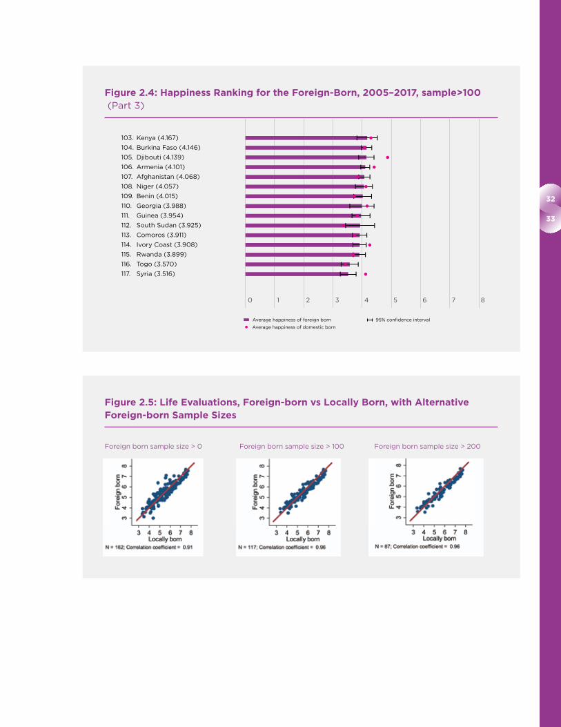
32
33
Figure 2.4: Happiness Ranking for the Foreign-Born, 2005–2017, sample>100 (Part 3)
103. Kenya (4.167)
104. Burkina Faso (4.146)
105. Djibouti (4.139)
106. Armenia (4.101)
107. Afghanistan (4.068)
108. Niger (4.057)
109. Benin (4.015)
110. Georgia (3.988)
111. Guinea (3.954)
112. South Sudan (3.925)
113. Comoros (3.911)
114. Ivory Coast (3.908)
115. Rwanda (3.899)
116. Togo (3.570)
117. Syria (3.516)
0 1 2 3 4 5 6 7 8
Average happiness of foreign born
Average happiness of domestic born
95% confidence interval
Figure 2.5: Life Evaluations, Foreign-born vs Locally Born, with Alternative Foreign-born Sample Sizes
Foreign born sample size > 0 Foreign born sample size > 100 Foreign born sample size > 200

World Happiness Report 2018
quite a range of experience. Among these 117
countries, there are 64 countries where immigrant
happiness is lower, averaging 94.5% of that of
the locally born; 48 countries where it is higher,
averaging 106% of the life evaluations of the
locally born; and five countries where the two
are essentially equal, with percentage differences
below 1%.26
The life evaluations of immigrants and of the
native-born are likely to depend on the extent
to which residents in each country are ready to
happily accept foreign migrants. To test this
possibility, we make use of a Migrant Acceptance
Index (MAI) developed by Gallup researchers27
and described in the Annex to this Report.28 Our
first test was to add the values of the MAI to the
first equation in Table 2.1. We found a positive
coefficient of 0.068, suggesting that immigrants,
local residents, or both, are happier in countries
where migrants are more welcome. An increase
of 2 points (about one standard deviation) on
the 9-point scale of migrant acceptance was
associated with average life evaluations higher
by 0.14 points on the 0 to 10 scale for life
evaluations. Is this gain among the immigrants
or the locally-born? We shall show later, when
we set up and test our main model for immigrant
happiness, that migrant acceptance makes both
immigrants and locally born happier, with the per
capita effects being one-third larger for immigrants.
But the fact that the foreign-born populations
are typically less than 15%, most of the total
happiness gains from migrant acceptance are
due to the locally born population, even if the
per-person effects are larger for the migrants.
Footprint effects, coupled with the fact that
happier countries are the major immigration
destinations, help to explain why immigrants
in happier countries are less happy than the
local population, while the reverse is true for
immigrants in less happy countries. Thus for
those 64 countries where immigrants have lower
life evaluations than the locally born, the average
life evaluation is 6.00, compared to 5.01 for the
48 countries where immigrants are happier than
the locally born. When the OECD studied the life
evaluations of immigrants in OECD countries,
they found that immigrants were less happy
than the locally born in three-quarters of their
member countries.29 That reflects the fact that
most of the happiest countries are also OECD
countries. In just over half of the non-OECD
countries, the foreign-born are happier than the
locally born.
Another way of looking for sources of possible
life evaluation differences between foreign-born
and locally born respondents is to see how
immigrants fare in different aspects of their lives.
All four of the social factors used in Table 2.1
show similar average values and cross-country
patterns for the two population groups, although
these patterns differ in interesting ways. The
correlation is lowest, although still very high
(at 0.91), for social support. It also has a lower
average value for the foreign-born, 79% of whom
feel they have someone to count on in times of
trouble, compared to 82% for the locally born
respondents. This possibly illustrates a conse-
quence of the uprooting effect of international
migration, as discussed in Chapter 3. The slope
of the relation is also slightly less than 45%,
showing that the immigrant vs locally born gap
for perceived social support is greatest for those
living in countries with high average values for
social support. Nonetheless, there is still a very
strong positive relation, so that immigrants
living in a country where the locally born have
internationally high values of social support feel
the same way themselves, even if in a slightly
muted way. When it comes to evaluations of the
institutional quality of their new countries,
immigrants rank these institutions very much as
do the locally-born, so that the cross-country
correlations of evaluations by the two groups are
very high, at 0.93 for freedom to make life
choices, and 0.97 for perceptions of corruption.
There are on average no footprint effects for
perceptions of corruption, as immigrants see less
evidence of corruption around them in their new
countries than do locally born, despite having
come, on average, from birth countries with
more corruption than where they are now living.
Generosity and freedom to make life choices are
essentially equal for immigrants and the locally
born, although slightly higher for the immigrants.
To a striking extent, the life evaluations of the
foreign-born are similar to those of the locally
born, as are the values of several of the key
social supports for better lives. But is the
happiness of immigrants and the locally born
affected to the same extent by these variables?
To assess this possibility, we divided the entire
accumulated individual Gallup World Poll
respondents 2005-2017, typically involving 1,000

34
35
observations per year in each country, into
separate foreign-born and domestically born
samples. As shown in Table 10 of Statistical
Appendix 2, immigrants and non-immigrants
evaluate their lives in almost identical ways, with
almost no significant differences.30
All of the evidence we have considered thus far
suggests that average life evaluations depend
first and foremost on the social and material
aspects of life in the communities and countries
where people live. Put another way, the substantial
differences across countries in average life
evaluations appear to depend more on the social
and material aspects of life in each community
and country than on characteristics inherent in
individuals. If this is true, then we would expect
to find that immigrants from countries with very
different average levels of life evaluations would
tend to have happiness levels much more like
those of others in their new countries than like
those of their previous friends, family and
compatriots still living in their original countries.
We can draw together the preceding lines of
evidence to propose and test a particular model
of immigrant happiness. Immigrant happiness
will be systematically higher in countries where
the local populations are happier, but the effect
will be less than one for one because of footprint
effects. Footprints themselves imply a positive
effect from the average happiness in the
countries from which the migrants came. Finally,
immigrant happiness will be happier in countries
where migrant acceptance is higher. All three
propositions are tested and confirmed by the
following equation, where average immigrant life
evaluations 2005-2017 (ladderimm) are ex-
plained by average happiness of the locally born
population (ladderdom), weighted average
happiness in the source countries (ladder-
source),31 and each country’s value for the Gallup
Migrant Acceptance Index as presented in the
Annex. The life evaluation used is the Cantril
ladder, as elsewhere in this chapter, with the
estimation sample including the 107 countries
that have more than 100 immigrant survey
responders and a value for the Migrant
Acceptance Index.
Ladderimm = 0.730 ladderdom +
(0.033)
0.243 laddersource +
(0.057)
0.049 migrant acceptance
(0.014)
Adjusted R2=0.941 n=107
All parts of the framework are strongly supported
by the results. It is also interesting to ask what
we can say about the effects of immigration on
the locally-born population. We have already
seen that immigrants more often move to happier
countries, as evidenced by the strong positive
simple correlation between immigrant share and
national happiness (r=+0.45). We cannot simply
use this to conclude also that a higher immigrant
share makes the domestic population happier. To
answer that question appropriately, we need to
take proper account of the established sources
of well-being. We can do this by adding the
immigrant share to a cross-sectional equation
explaining the life evaluations of the locally-born
by the standard variables used in Table 2.1. When
this is done, the estimated effect of the immigrant
population share32 is essentially zero.
A similar test using the same framework to
explain cross-country variations of the life evalua-
tions of immigrants also showed no impact from
the immigrant share of the population. The same
framework also showed that GDP per capita has
no effect on the average life evaluations, once the
effect flowing through the average life evaluations
of the locally born is taken into account.33
We can use the same framework to estimate the
effects of migrant acceptance on the happiness
of the host populations, by adding the index to a
cross-sectional equation explaining the average
life evaluations of the host populations 2005-
2017 by the six key variables of Table 2.1 plus the
Migrant Acceptance Index. The Migrant Acceptance
Index attracts a coefficient of 0.075 (SE=0.028),
showing that those who are not themselves
immigrants are happier living in societies where
immigrant acceptance is higher. The total effect
of the Migrant Acceptance Index on immigrants
is slightly larger, as can be seen by combining
the direct effect from the equation shown above
(0.049) plus that flowing indirectly through the
life evaluations of the locally born (0.73*0.075),34
giving a total effect of 0.103.
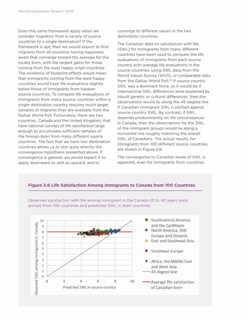
World Happiness Report 2018
Does this same framework apply when we
consider migration from a variety of source
countries to a single destination? If the
framework is apt, then we would expect to find
migrants from all countries having happiness
levels that converge toward the average for the
locally born, with the largest gains for those
coming from the least happy origin countries.
The existence of footprint effects would mean
that immigrants coming from the least happy
countries would have life evaluations slightly
below those of immigrants from happier
source countries. To compare life evaluations of
immigrants from many source countries within a
single destination country requires much larger
samples of migrants than are available from the
Gallup World Poll. Fortunately, there are two
countries, Canada and the United Kingdom, that
have national surveys of life satisfaction large
enough to accumulate sufficient samples of
the foreign-born from many different source
countries. The fact that we have two destination
countries allows us to test quite directly the
convergence hypothesis presented above. If
convergence is general, we would expect it to
apply downward as well as upward, and to
converge to different values in the two
destination countries.
The Canadian data on satisfaction with life
(SWL) for immigrants from many different
countries have been used to compare the life
evaluations of immigrants from each source
country with average life evaluations in the
source countries, using SWL data from the
World Values Survey (WVS), or comparable data
from the Gallup World Poll.35 If source country
SWL was a dominant force, as it would be if
international SWL differences were explained by
inbuilt genetic or cultural differences, then the
observations would lie along the 45-degree line
if Canadian immigrant SWL is plotted against
source-country SWL. By contrast, if SWL
depends predominantly on life circumstances
in Canada, then the observations for the SWL
of the immigrant groups would lie along a
horizontal line roughly matching the overall
SWL of Canadians. The actual results, for
immigrants from 100 different source countries,
are shown in Figure 2.6.
The convergence to Canadian levels of SWL is
apparent, even for immigrants from countries
Figure 2.6 Life Satisfaction Among Immigrants to Canada from 100 Countries
Observed satisfaction with life among immigrant in the Canada (0 to 40 years since
arrival) from 100 countries and predicted SWL in their countries
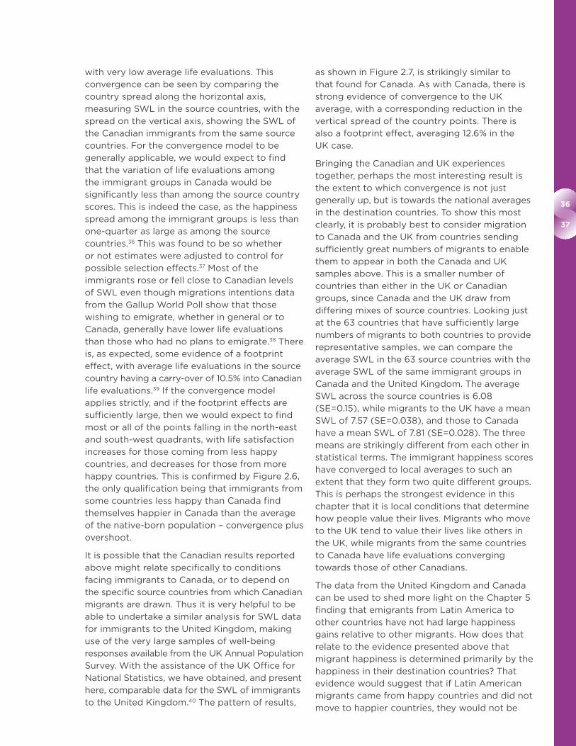
36
37
with very low average life evaluations. This
convergence can be seen by comparing the
country spread along the horizontal axis,
measuring SWL in the source countries, with the
spread on the vertical axis, showing the SWL of
the Canadian immigrants from the same source
countries. For the convergence model to be
generally applicable, we would expect to find
that the variation of life evaluations among
the immigrant groups in Canada would be
significantly less than among the source country
scores. This is indeed the case, as the happiness
spread among the immigrant groups is less than
one-quarter as large as among the source
countries.36 This was found to be so whether
or not estimates were adjusted to control for
possible selection effects.37 Most of the
immigrants rose or fell close to Canadian levels
of SWL even though migrations intentions data
from the Gallup World Poll show that those
wishing to emigrate, whether in general or to
Canada, generally have lower life evaluations
than those who had no plans to emigrate.38 There
is, as expected, some evidence of a footprint
effect, with average life evaluations in the source
country having a carry-over of 10.5% into Canadian
life evaluations.39 If the convergence model
applies strictly, and if the footprint effects are
sufficiently large, then we would expect to find
most or all of the points falling in the north-east
and south-west quadrants, with life satisfaction
increases for those coming from less happy
countries, and decreases for those from more
happy countries. This is confirmed by Figure 2.6,
the only qualification being that immigrants from
some countries less happy than Canada find
themselves happier in Canada than the average
of the native-born population – convergence plus
overshoot.
It is possible that the Canadian results reported
above might relate specifically to conditions
facing immigrants to Canada, or to depend on
the specific source countries from which Canadian
migrants are drawn. Thus it is very helpful to be
able to undertake a similar analysis for SWL data
for immigrants to the United Kingdom, making
use of the very large samples of well-being
responses available from the UK Annual Population
Survey. With the assistance of the UK Office for
National Statistics, we have obtained, and present
here, comparable data for the SWL of immigrants
to the United Kingdom.40 The pattern of results,
as shown in Figure 2.7, is strikingly similar to
that found for Canada. As with Canada, there is
strong evidence of convergence to the UK
average, with a corresponding reduction in the
vertical spread of the country points. There is
also a footprint effect, averaging 12.6% in the
UK case.
Bringing the Canadian and UK experiences
together, perhaps the most interesting result is
the extent to which convergence is not just
generally up, but is towards the national averages
in the destination countries. To show this most
clearly, it is probably best to consider migration
to Canada and the UK from countries sending
sufficiently great numbers of migrants to enable
them to appear in both the Canada and UK
samples above. This is a smaller number of
countries than either in the UK or Canadian
groups, since Canada and the UK draw from
differing mixes of source countries. Looking just
at the 63 countries that have sufficiently large
numbers of migrants to both countries to provide
representative samples, we can compare the
average SWL in the 63 source countries with the
average SWL of the same immigrant groups in
Canada and the United Kingdom. The average
SWL across the source countries is 6.08
(SE=0.15), while migrants to the UK have a mean
SWL of 7.57 (SE=0.038), and those to Canada
have a mean SWL of 7.81 (SE=0.028). The three
means are strikingly different from each other in
statistical terms. The immigrant happiness scores
have converged to local averages to such an
extent that they form two quite different groups.
This is perhaps the strongest evidence in this
chapter that it is local conditions that determine
how people value their lives. Migrants who move
to the UK tend to value their lives like others in
the UK, while migrants from the same countries
to Canada have life evaluations converging
towards those of other Canadians.
The data from the United Kingdom and Canada
can be used to shed more light on the Chapter 5
finding that emigrants from Latin America to
other countries have not had large happiness
gains relative to other migrants. How does that
relate to the evidence presented above that
migrant happiness is determined primarily by the
happiness in their destination countries? That
evidence would suggest that if Latin American
migrants came from happy countries and did not
move to happier countries, they would not be
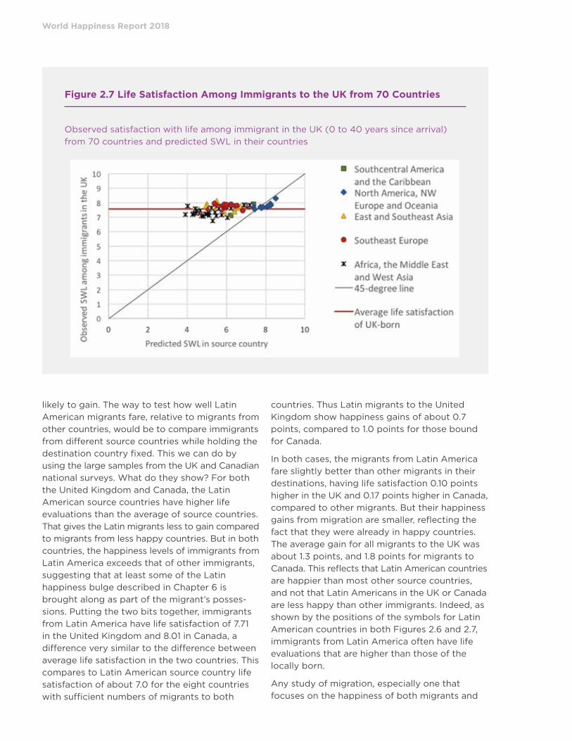
World Happiness Report 2018
likely to gain. The way to test how well Latin
American migrants fare, relative to migrants from
other countries, would be to compare immigrants
from different source countries while holding the
destination country fixed. This we can do by
using the large samples from the UK and Canadian
national surveys. What do they show? For both
the United Kingdom and Canada, the Latin
American source countries have higher life
evaluations than the average of source countries.
That gives the Latin migrants less to gain compared
to migrants from less happy countries. But in both
countries, the happiness levels of immigrants from
Latin America exceeds that of other immigrants,
suggesting that at least some of the Latin
happiness bulge described in Chapter 6 is
brought along as part of the migrant’s posses-
sions. Putting the two bits together, immigrants
from Latin America have life satisfaction of 7.71
in the United Kingdom and 8.01 in Canada, a
difference very similar to the difference between
average life satisfaction in the two countries. This
compares to Latin American source country life
satisfaction of about 7.0 for the eight countries
with sufficient numbers of migrants to both
countries. Thus Latin migrants to the United
Kingdom show happiness gains of about 0.7
points, compared to 1.0 points for those bound
for Canada.
In both cases, the migrants from Latin America
fare slightly better than other migrants in their
destinations, having life satisfaction 0.10 points
higher in the UK and 0.17 points higher in Canada,
compared to other migrants. But their happiness
gains from migration are smaller, reflecting the
fact that they were already in happy countries.
The average gain for all migrants to the UK was
about 1.3 points, and 1.8 points for migrants to
Canada. This reflects that Latin American countries
are happier than most other source countries,
and not that Latin Americans in the UK or Canada
are less happy than other immigrants. Indeed, as
shown by the positions of the symbols for Latin
American countries in both Figures 2.6 and 2.7,
immigrants from Latin America often have life
evaluations that are higher than those of the
locally born.
Any study of migration, especially one that
focuses on the happiness of both migrants and
Figure 2.7 Life Satisfaction Among Immigrants to the UK from 70 Countries
Observed satisfaction with life among immigrant in the UK (0 to 40 years since arrival)
from 70 countries and predicted SWL in their countries
38
39
non-migrants, leads naturally to considerations
of the possible linkages between migration and
world happiness. We have done our best to
assemble the available data on the life evaluations
of migrants and non-migrants alike. Many
countries, especially those where people
evaluate their lives highly, have many would-be
migrants, on top of the humanitarian need to
somehow accommodate those whose lives in
their birth countries have become impossibly
difficult. Is migration making the world as a
whole happier or unhappier? Is there any pre-
ferred level of migration that will best serve to
provide opportunities for newcomers, to build
positive linkages among countries, and accom-
modate the need to find new homes for refu-
gees, while still maintaining and improving the
quality of the social fabric that supports better
lives? There is no easy answer to this question.
Are countries with higher immigration rates
thereby happier places to live, for migrants and
non-migrants alike? We have already seen that
most migration is from less happy to happier
places, so we expect to find that happier countries
do tend to have higher foreign-born population
shares. But that does not answer the question,
since in this case the migration is responding to
the differences in happiness and other aspects of
life, and is probably not responsible for creating
the differences. One limited way of answering
the question might be to add the foreign-born
population share for each country to the equation
we used in Table 2.1 to explain annual observations
of life evaluations in the sample of 157 countries
using data from 2005 through 2017. We did this,
and there was no significant effect. Alternatively,
and preferably, we repeated that analysis using
country fixed effects, so that any influence we
found would be free of country effects, and
would instead look for happiness changes
within countries in response to changes in their
shares of foreign-born population. We found an
insignificant negative effect that remained
both negative and insignificant under several
alternative specifications.41 There are only limited
data for changes in each country’s shares of
foreign-born population, and many other factors
that might be in play, so there can be no firm
conclusions drawn from these limited experiments.
As described previously, we also tested whether
international differences in accumulated net
immigration (as measured by the foreign-born
population share) had any impact in explaining
cross-country variations in the average 2005-
2017 life evaluations for either the immigrant or
locally born populations, once account is taken
of the six main determinants of life evaluations.
We found no effect, either positive or negative.
Conclusions
This chapter, as usual, has a double focus. The
first half of the chapter presented our latest
ranking of countries according to their average
life evaluations over the previous three years,
followed by a ranking of changes in life evaluations
from 2008-2010 to 2015-2017. The second half
turned the focus to international migration,
ranking countries by the average life evaluations
of all the foreign-born respondents to the Gallup
World Poll between 2005 and 2017.
The rankings of country happiness are based this
year on the pooled results from Gallup World
Poll surveys from 2015-2017, and show both
change and stability. There is a new top ranking
country, Finland, but the top ten positions are
held by the same countries as in the last two
years, although with some swapping of places.
Four different countries have held top spot since
2015 – Switzerland, Denmark, Norway and now
Finland.
All the top countries tend to have high values for
all six of the key variables that have been found
to support well-being: income, healthy life
expectancy, social support, freedom, trust and
generosity, to such a degree that year to year
changes in the top ranking are to be expected.
This year the happiness changes reported are
those from 2008-2010, in the immediate aftermath
of the financial crisis of 2007-2008; to the most
recent years, covering 2015-2017. The winner of
the change category was Togo, as it posted the
largest gain since 2008-2010, almost 1.2 points. It
was the lowest ranked country in World Happiness
Report 2015 and now ranks 17 places higher.
Other signal success stories, countries with
average life evaluation gains of more than a full
point on the 0 to 10 scale since 2008-2010,
include Latvia, Bulgaria and Sierra Leone. The
largest happiness losses since 2008-2010 were
in Ukraine, Yemen, Syria, Malawi and Venezuela,
with drops over 1 point in each case, the largest
fall being almost 2.2 points in Venezuela.

World Happiness Report 2018
Five of this report’s seven chapters deal primarily
with migration. Perhaps the most striking finding
of the whole report is that a ranking of countries
according to the happiness of their immigrant
populations is almost exactly the same as for the
rest of the population. The immigrant happiness
rankings are based on the full span of Gallup
data from 2005 to 2017, which is sufficient to
have 117 countries with more than 100 immigrant
respondents. Finland picks up a second gold
medal here, as home to the world’s happiest
immigrants.
The closeness of the two rankings shows that
immigrant happiness depends predominantly on
the quality of life where they now live, illustrating
a general pattern of convergence. Happiness can
change, and does change, according to the
quality of the society in which people live.
Immigrant happiness, like that of the locally born
depends on a range of features of the social
fabric, extending far beyond the higher incomes
traditionally thought to inspire and reward
migration. Once the overall quality of life is taken
into account (with income given its due weight
as one of the six factors), there is no happiness
gain from moving to a higher income country.
That has been tested, but is already suggested
by the countries with the happiest immigrants
are not the richest countries, but instead the
countries with a more balanced set of social and
institutional supports for better lives.
While convergence to local happiness levels is
quite rapid, it is not complete, as there is a
‘footprint’ effect based on the happiness in each
source country. This effect ranges from 10% to
25%. This footprint effect, coupled with the fact
that most migration is from less happy to happier
countries, explains why, although on average
across the world immigrant happiness is very
close to that of the locally born, it is less than
that of the locals in the happiest countries and
greater in the less happy countries.
Since immigrants tend on average to have life
evaluations close to those of people already
living in destination countries, does this suggest
that world happiness would be higher if there
were more migration from unhappy to happy
places? Although this question underlies many
current political debates, the available evidence
is not yet good enough to provide anything like
definitive conclusions. What does seem apparent,
as will be shown in more detail in Chapter 3, is
that every migration pathway, and each migration
flow, has its own story, with often diverging
well-being outcomes for the migrants, their new
communities, and the communities left behind.
We have shown that the happiest counties have
higher than world average shares of foreign-born
population. The top 10 countries in the Figure 2.2
rankings of 2015-2017 life evaluations had foreign-
born population shares averaging 18% in 2015,
more than twice the global country average of
8.7%, and covering a wide range, from 6% to
30%. These same countries also had the happiest
foreign-born populations. Based on the average
life evaluations 2005-2017 for foreign-born
respondents (in Figure 2.4), the same countries
dominated the top spots in the world rankings,
with all of the top 10 countries in the overall
happiness rankings 2015-2017 being in the top
11 countries for 2005-2017 happiness of their
foreign-born populations. This is due to a
combination of factors: their attractiveness to
international migrants, their willingness to accept
migrants, and their ability to achieve integration
in ways that maintain life evaluations for both
immigrants and the locally born.
Helsinki, Copenhagen and Reykjavik are already
very international places. What is for them, and
for the world, the right scale and pattern of
future migration to help support and build
international cooperation of a sort that will help
the billions of people still living in misery? These
are not the world’s happiest cities because of
where they are, but because their residents
have over many decades built levels of trust,
connections, cooperation and innovation
sufficient to deliver satisfying lives for them-
selves, and to be in a position to help others do
the same. What is needed is to look behind the
average life evaluations to see what makes for
better lives, and to help others to make progress
in improving their own lives. International migra-
tion, with its increasing two-way flows, is likely to
continue to provide international human linkages
and shared sympathies sufficient to support
knowledge transfers of the sort that are needed.
But migration flows not properly managed and
digested have the potential for destroying trust
and inflaming anti-immigrant views.
Similar questions arise when city-level happiness
is ranked in countries that have sufficiently great
samples of data to make such comparisons

40
41
feasible. One immediate response among readers
and commentators is to suggest that people
should move to a happier community in order to
make themselves happier. On reflection, when
they see the nature of the social connections,
and the quality of communities, governments
and workplaces that underlie these happier lives,
they see that the right answer is not to move to
the happier communities but instead to learn and
apply the lessons and inspirations that underlie
their happiness. Happiness is not something
inherently in short supply, like gold, inciting
rushes to find and much conflict over ownership.
My gold cannot be your gold. But happiness,
unlike gold, can be created for all, and can be
shared without being scarce for those who give.
It even grows as it is shared.
World Happiness Report 2018
Endnotes
1 Gallup weights sum up to the number of respondents from each country. To produce weights adjusted for population size in each country for the period of 2015-2017, we first adjust the Gallup weights so that each country has the same weight (one-country-one-vote) in the period. Next we multiply total population aged 15+ in each country in 2016 by the one-country-one-vote weight. To simplify the analysis, we use population in 2016 for the period of 2015-2017 for all the countries/regions. Total population aged 15+ is equal to the total population minus the amount of population aged 0-14. Data are mainly taken from WDI released by the World Bank in September 2017. Specifically, the total population and the proportion of population aged 0-14 are taken from the series “Population ages 0-14 (percent of total)” and “Population, total” respectively from WDI. There are a few regions lack of data in WDI, such as Somaliland, Kosovo, and Taiwan. In this case, other sources of data are used if available. The share of population aged 0-14 is missing in WDI, we thus use the data from CIA’s World Fact Book, 25.01% to calculate the amount of adult population. The total population in Taiwan in 2016 is 23,540,000, and the aged 15+ is 20,398,000 in 2015 (Statistical Yearbook of the Republic of China 2016, Table 3). There are no reliable data on population and age structure in Somaliland region, therefore it is not included in the calculation of world or regional distributions.
2 See, for example, Atkinson (2015), Atkinson and Bourguignon (2014), , Kennedy, Lochner, and Prothrow-Stith (1997), Keeley (2015), OECD (2015), Neckerman and Torche (2007), and Piketty (2014).
3 See Helliwell, Huang, and Wang (2016). See also Goff, Helliwell, and Mayraz (2016), Gandelman and Porzekanski (2013), Kalmijn and Veenhoven (2005).
4 See, for example, Evans, Barer, and Marmor (1997), Marmot, Ryff, Bumpass, Shipley, and Marks (1994), and Marmot (2005).
5 See Corak (2013).
6 See Table 17 in Statistical Appendix 1.
7 The statistical appendix contains alternative forms without year effects (Table 14 of Appendix 1), and a repeat version of the Table 2.1 equation showing the estimated year effects (Table 9 of Appendix 1). These results confirm, as we would hope, that inclusion of the year effects makes no significant difference to any of the coefficients.
8 As shown by the comparative analysis in Table 8 of Appendix 1.
9 The definitions of the variables are shown in Technical Box 1, with additional detail in the online data appendix.
10 This influence may be direct, as many have found, e.g. De Neve, Diener, Tay, and Xuereb (2013). It may also embody the idea, as made explicit in Fredrickson’s broaden-and-build theory (Fredrickson, 2001), that good moods help to induce the sorts of positive connections that eventually provide the basis for better life circumstances.
11 See, for example, Danner, Snowdon, and Friesen (2001), Cohen, Doyle, Turner, Alper, and Skoner (2003), and Doyle, Gentile, and Cohen (2006).
12 We put the contributions of the six factors as the first elements in the overall country bars because this makes it easier to see that the length of the overall bar depends only on the average answers given to the life evaluation question. In World Happiness Report 2013 we adopted a different ordering, putting the combined Dystopia+residual elements on the left of each bar to make it easier to compare the sizes of residuals across countries. To make that comparison equally possible in subsequent World Happiness Reports, we include the alternative form of the figure in the online Statistical Appendix 1 (Appendix Figures 7-9).
13 These calculations are shown in detail in Table 19 of the online Statistical Appendix 1.
14 The prevalence of these feedbacks was documented in Chapter 4 of World Happiness Report 2013, De Neve, Diener, Tay, and Xuereb (2013).
15 The coefficients on GDP per capita and healthy life expectancy are affected even less, and in the opposite direction in the case of the income measure, being increased rather than reduced, once again just as expected. The changes are tiny because the data come from other sources, and are unaffected by our experiment. However, the income coefficient does increase slightly, since income is positively correlated with the other four variables being tested, so that income is now able to pick up a fraction of the drop in influence from the other four variables. We also performed an alternative robustness test, using the previous year’s values for the four survey-based variables. This also avoids using the same respondent’s answers on both sides of the equation, and produces similar results, as shown in Table 13 of the Statistical Appendix 1. The Table 13 results are very similar to the split-sample results shown in Tables 11 and 12, and all three tables give effect sizes very similar to those in Table 2.1 in reported in the main text.
16 The data and calculations are shown in detail in Table 20 of the Statistical Appendix 1. Annual per capita incomes average $46,000 in the top 10 countries, compared to $1,500 in the bottom 10, measured in international dollars at purchasing power parity. For comparison, 95% of respondents have someone to count on in the top 10 countries, compared to 58% in the bottom 10. Healthy life expectancy is 72 years in the top 10, compared to 53 years in the bottom 10. 93% of the top 10 respondents think they have sufficient freedom to make key life choices, compared to 62% in the bottom 10. Average perceptions of corruption are 34%in the top 10, compared to 73% in the bottom 10.
17 Actual and predicted national and regional average 2015-2017 life evaluations are plotted in Figure 16 of the Statistical Appendix 1. The 45-degree line in each part of the Figure shows a situation where the actual and predicted values are equal. A predominance of country dots below the 45-degree line shows a region where actual values are below those predicted by the model, and vice versa. East Asia provides an example of the former case, and Latin America of the latter.
18 For example, see Chen, Lee, and Stevenson (1995).
19 One slight exception is that the negative effect of corruption is estimated to be slightly larger, although not significantly so, if we include a separate regional effect variable for Latin America. This is because corruption is worse than average in Latin America, and the inclusion of a special Latin American variable thereby permits the corruption coefficient to take a higher value.

42
43
20 The number of languages used in a country includes all those spoken by more than 5% of the population.
21 As noted in Technical Box 3 in Chapter 2 of World Happiness Report 2017, the Gulf Cooperation Council (GCC) countries are a special case in three ways. First they have very high foreign-born population shares. Second, their overall country estimates are adjusted to reflect outside estimates of the non-national population, and third, Gallup Polls in those countries were offered in Arabic only prior to 2014, so that their non-national respondents in the earlier years were almost entirely drawn from other Arab-speaking countries. In Figure 2.4 we report the foreign-born ladder scores using all available years for all countries, while in Technical Box 3 of WHR 2017 the figures are based only on 2014 and later, permitting a comparison of the two procedures. For most of the GCC countries the estimates are quite similar, differences presumably resulting from the relative evaluations and numbers of the Arab-speaking and English-speaking respondents.
22 5.7%=100*(93/(93+1540)).
23 The correlation is 0.9 between the two country-level estimates of foreign-born population shares.
24 There is a similar ranking of immigrant life evaluations for the OECD countries in Figure 3.21 of OECD (2017).
25 Regressing the immigrant share, as a proportion, on the average ladder score of the locally born gives a coefficient of 0.058 (t=5.5).
26 This is based on the ratios of foreign-born to locally born life evaluation averages for the 117 countries where there are more than 100 foreign-born respondents in the 2005-2017 data period. The ratios are averaged for each country to the nearest percentage point – hence the equality for five countries.
27 The Migrant Acceptance Index is a proprietary index developed by Gallup, based on items it asks in its Gallup World Poll surveys. Their initial analysis of the data may be found at: http://news.gallup.com/poll/216377/new-index-shows-least-accepting-countries-migrants.aspx. The definition of the index, and its values for the most accepting and non-accepting countries, are shown in the Annex to this report by Esipova, Ray, Fleming, and Pugliese (2018).
28 There is only a single value of the index for each country, which then has to be repeated for each country-year in the panel.
29 See OECD (2017), Figure 3.21.
30 A similar conclusion follows, as also shown in Statistical Appendix 2, if we use national average data in separate cross-sectional equations for the foreign-born and locally born sub-populations. In this instance we need to do a pure cross section rather than the panel approach used in Table 2.1, because the samples of the foreign-born in each annual sample of 1,000 respondents are much too small to enable regressions using country-year data.
31 The average life evaluations of the locally born and the weighted average source country life evaluations also make use of the entire 2005-2017 sample. The Migrant Acceptance Index is a single value for each country, as described in Esipova et al. (2018).
32 The simple correlation between the ratio and the immigrant share of the population is significantly negative, but disappears when the happiness of the locally born is controlled for. This is because, as we have already shown, foreign-born population shares are higher in countries with happier locally born populations.
33 This is consistent with Hendriks and Bartram (2016), who find economic conditions to be incomplete as explanations of migrant happiness. Our results are testing whether national income is more important for migrant than for non-migrant happiness, and we find that it is not, since there is a zero coefficient on log GDP per capita when added to an equation explaining immigrant happiness by native-born happiness and the happiness in their source countries. Hence the non-economic sources of life evaluations are equally important for both immigrant and locally born respondents.
34 The effect flowing through domestic happiness is equal to the effect in the domestic happiness equation (0.075) times the effect of domestic happiness on immigrant happiness (0.73). The total effect on immigrants is the sum of the direct and indirect elements (0.049 + 0.73*.075 = 0.103).
35 The use of the Gallup World Poll data permits more countries to be considered, as it covers many more countries than does the World Values Survey. Helliwell, Bonikowska, and Shiplett (2018) show comparable results using WVS and Gallup estimates for source country life evaluations. An empirically estimated conversion factor is used to convert Gallup ladder data to SWL equivalents, based on Gallup data from the year when ladder and SWL questions were both asked of all respondents.
36 More precisely, the standard deviation across countries is 1.17 among the source countries, and 0.24 among the immigrant groups. The Canadian distribution is about a higher mean, as the average SWL in the 100 source countries is 6.06, compared to 7.84 among the immigrant groups.
37 See Helliwell et al. (2018). A similar matching process, with similar results, is available for a smaller number of countries in Frank, Hou, and Schellenberg (2016).
38 See Helliwell et al. (2018, Figure 1).
39 That is, if the average SWL of immigrants from each of the 100 source countries is regressed on the average estimated SWL in those 100 countries, the estimated coefficient is 0.105 (t=5.8).
40 The ONS has posted the data for public use on: https://www.ons.gov.uk/peoplepopulationandcommunity/wellbeing/adhocs/007955estimatesofpersonalwellbeing-brokendownbycountryofbirthfromtheukannualpopulation-surveyaps
41 For example, regressing country averages of immigrant life evaluations on the corresponding averages for the locally born and each country’s share of foreign-born population shows a slight but insignificant negative effect for the foreign-born population share.

World Happiness Report 2018
References
Atkinson, A. B. (2015). Inequality: What can be done? Cambridge: Harvard University Press.
Atkinson, A. B., & Bourguignon, F. (2014). Handbook of income distribution (Vols. 2A &2B). Elsevier.
Chen, C., Lee, S. Y., & Stevenson, H. W. (1995). Response style and cross-cultural comparisons of rating scales among East Asian and North American students. Psychological Science, 6(3), 170-175.
Cohen, S., Doyle, W. J., Turner, R. B., Alper, C. M., & Skoner, D. P. (2003). Emotional style and susceptibility to the common cold. Psychosomatic Medicine, 65(4), 652-657.
Corak, M. (2013). Income inequality, equality of opportunity, and intergenerational mobility. The Journal of Economic Perspectives, 27(3), 79-102.
Danner, D. D., Snowdon, D. A., & Friesen, W. V. (2001). Positive emotions in early life and longevity: findings from the nun study. Journal of Personality and Social Psychology, 80(5), 804.
De Neve, J. E., Diener, E., Tay, L., & Xuereb, C. (2013). The objective benefits of subjective well-being. In J. F. Helliwell, R. Layard, & J. Sachs (Eds.), World happiness report 2013 (pp. 54-79). New York: UN Sustainable Development Solutions Network.
Doyle, W. J., Gentile, D. A., & Cohen, S. (2006). Emotional style, nasal cytokines, and illness expression after experimental rhinovirus exposure. Brain, Behavior, and Immunity, 20(2), 175-181.
Esipova, N., Ray, J., Fleming, J., & Pugliese, A. (2018). Migrant Acceptance Index: Do migrants have better lives in countries that accept them? Annex to World happiness report 2018.
Evans, R. G., Barer, M. L., & Marmor, T. R. (Eds.) (1994). Why are some people healthy and others not? The determinants of the health of populations. New York: De Gruyter.
Frank, K., Hou, F., & Schellenberg, G. (2016). Life satisfaction among recent immigrants in Canada: comparisons to source-country and host-country populations. Journal of Happiness Studies, 17(4): 1659-1680. doi:10.1007/s10902-015-9664-2.
Fredrickson, B. L. (2001). The role of positive emotions in positive psychology: The broaden-and-build theory of positive emotions. American psychologist, 56(3), 218-226.
Gandelman, N., & Porzecanski, R. (2013). Happiness inequality: How much is reasonable? Social Indicators Research, 110(1), 257-269.
Goff, L., Helliwell, J., & Mayraz, G. (2016). The welfare costs of well-being inequality. NBER Working Paper no. 21900.
Helliwell, J. F., Bonikowska, A. & Shiplett, H. (2018). Migration as a test of the happiness set point hypothesis: Evidence from immigration to Canada and the United Kingdom. NBER Working Paper no. 22601 (original version 2016, revised to include the United Kingdom, March 2018).
Helliwell, J. F., Huang, H., & Wang, S. (2016). New evidence on trust and well-being. NBER Working Paper no. 22450.
Hendriks, M., & Bartram, D. (2016). Macro-conditions and immigrants’ happiness: Is moving to a wealthy country all that matters? Social Science Research, 56, 90-107.
Kalmijn, W., & Veenhoven, R. (2005). Measuring inequality of happiness in nations: In search for proper statistics. Journal of Happiness Studies, 6(4), 357-396.
Kawachi, I., & Berkman, L. (2000). Social cohesion, social capital, and health. In L. F. Berkman & I. Kawachi (Eds.), Social epidemiology (pp. 174-190). New York: Oxford University Press.
Kawachi, I., Kennedy, B. P., Lochner, K., & Prothrow-Stith, D. (1997). Social capital, income inequality, and mortality. American Journal of Public Health, 87(9), 1491-1498.
Keeley, B. (2015). Income inequality: The gap between rich and poor. OECD Insights, Paris: OECD Publishing.
Marmot, M. (2005). Social determinants of health inequalities. The Lancet, 365(9464), 1099-1104.
Marmot, M., Ryff, C. D., Bumpass, L. L., Shipley, M., & Marks, N. F. (1997). Social inequalities in health: Next questions and converging evidence. Social Science & Medicine, 44(6), 901-910.
Neckerman, K. M., & Torche, F. (2007). Inequality: Causes and consequences. Annual Review of Sociology, 33, 335-357.
OECD (2015). In it together: Why less inequality benefits all. Paris: OECD Publishing. DOI: http://dx.doi.org/10.1787/9789264235120-en.
OECD (2017). How’s life?: Measuring well-being. Paris: OECD Publishing.
Piketty, T. (2014). Capital in the 21st Century. Cambridge: Harvard University Press.

44
45Chapter 3
Do International Migrants Increase Their Happiness and That of Their Families by Migrating?
Martijn Hendriks, Erasmus Happiness Economics Research Organisation (EHERO), Erasmus University Rotterdam
Martijn J. Burger, Erasmus Happiness Economics Research Organisation (EHERO), Department of Applied Economics, and Tinbergen Institute, Erasmus University Rotterdam
Julie Ray, Gallup
Neli Esipova, Gallup
The authors are grateful for the helpful comments and valuable suggestions of Milena Nikolova, John F. Helliwell, and Richard Layard.
World Happiness Report 2018
The considerable happiness differences between
countries suggest that migrating to another
country provides for many people a major
opportunity to obtain a happier life. However,
negative migrant experiences are common,
including exploitation, social exclusion, home-
sickness, and unsuccessful socioeconomic
assimilation.1 This raises important questions in
our globalizing world, where more than 700
million people currently say they would like to
move permanently to another country if they
had the opportunity,2 and where the international
migrant population is expected to increase from
the current 250 million to an estimated 400
million people in 2050.3 Do migrants generally
gain happiness from moving to another country?
In what specific migration flows do migrants gain
happiness from moving abroad? Do the short-
term and long-term impacts of migration on
migrants’ happiness differ? What is the impact
of migration on the happiness of families
left behind?
We assess these questions in a global context
using Gallup World Poll (GWP) data including
more than 36,000 first-generation migrants from
over 150 countries and territories. By addressing
these questions empirically, this chapter is
intended to develop globally comparable
information about how migration affects the
happiness of migrants and their families. The
outcomes in both the affective and cognitive
dimensions of happiness will be considered.
The affective dimension refers to the frequency
of experiencing pleasant moods and emotions
as opposed to unpleasant ones, whereas the
cognitive dimension refers to a person’s
contentment and satisfaction with life.4
Approximately 10% of international migrants
are considered refugees who were forced to
migrate by external circumstances such as war,
persecution, or natural disasters.5 The other 90%
of international migrants are believed to move
largely voluntarily. Voluntary migrants mention
a variety of motives for migration, including
economic gain, career or study opportunities,
living closer to family, or a more livable or
suitable environment (e.g., more religious or
political freedom). On the most general level,
however, these concrete motives are different
ways migrants attempt to improve their own or
their families’ lives.6 Empirical research shows
that, when making important decisions such as
migration decisions, most people tend to choose
the option they think will make them or their
families happiest.7 This suggests that migrants
move particularly to improve their own or their
families’ lives in terms of happiness, with the
exception of refugees who move primarily to
secure their lives. Conceptually, then, happiness,
which is often used synonymously with subjective
well-being, provides valuable information about
migrant well-being.
The above considerations imply that voluntary
migrants anticipate that migration will lead to
improved well-being for themselves and/or
their families. Many migrants will surely experience
considerable happiness gains, particularly those
who meet basic subsistence needs by migrating,
as basic needs such as economic security and
safety are vital conditions for happiness.8 Migrants
moving to more developed countries may also
experience major gains in other important
well-being domains, such as freedom, education,
and economic welfare.9
It should come as no surprise, however, to find
that some migrants have not become happier
following migration. Migration is associated with
severe costs in other critical well-being domains,
particularly those relating to social and esteem
needs. Separation from friends and family, social
exclusion in the host country (e.g., discrimination),
and decreased social participation due to linguistic
and cultural barriers are typical social costs of
migration that frequently result in experiences
of social isolation, loneliness, and impaired social
support among migrants.10 Migration also often
entails a lower position in the social hierarchy, a
sense of dislocation, and acculturative stress
(cultural clashes and identity issues).11 Additionally,
happiness gains may falter over time because
people tend to adapt more to the typical benefits
of migration, such as improvements in economic
welfare, than to migration’s typical costs, such
as leaving behind one’s social and cultural
environment.12
Migration decisions are complicated by major
information constraints. Most prospective
migrants have never been in their intended
destination country. They necessarily resort to
information from the media or their personal
social network. However, these sources tend to
provide limited and positively biased information;
for example, migrants tend to be hesitant about

46
47
revealing their disappointing migration outcomes
to people in their home country.13 In essence,
prospective migrants must make one of the most
important and difficult decisions of their lives
based on limited knowledge of its consequences.
Imperfect decisions may also follow from
inaccurately weighing the importance of the
anticipated advantages and disadvantages of
migrating. Placing disproportionate weight on
certain aspects of the outcome may be common,
since human susceptibility to deviations from a
standard of rationality is well-documented in the
social sciences.14 Specifically, people are believed
to put excessive weight on satisfying salient
desires, most notably economic gain, at a cost
to more basic needs such as social needs.15 These
beliefs are inspired by the weak correlation between
economic welfare and happiness for people who
have sufficient money to make ends meet.16
Migration may thus be a misguided endeavour for
some migrants who move in search of a better
life,17 which signals the need to evaluate whether
migrants are truly better off after migration.
Evaluating the outcomes of migration is compli-
cated, however, by the rarity of experimental
studies and panel studies tracking international
migrants across international borders. Existing
work evaluating migrants’ happiness outcomes
is mostly limited to comparing the happiness of
migrants with that of demographically similar
people living in a migrant’s home country
(matched stayers).18 The happiness of matched
stayers reflects what the migrant’s happiness
would have been like had they not migrated,
which implies that migrants benefit from
migration if they report higher happiness levels
than matched stayers.19 This methodology has
limited leverage in estimating the causal impact
of migration because the non-random selection
of people into migration is not fully captured by
the comparison of demographically similar
migrants and stayers. For example, compared
with stayers, migrants tend to be less risk-averse,
to have a higher achievement motivation and
lower affiliation motivation, and to differ in terms
of pre-migration skills and wealth.20 Moreover,
people who are relatively unhappy given their
socio-economic conditions are more willing to
migrate.21 Such unobserved pre-migration differ-
ences between migrants and stayers may bias
the estimated impact of migration when using
simple comparisons of migrants and stayers.
The current literature generally reports happiness
gains for migrants moving to more developed
countries, whereas non-positive happiness
outcomes are observed particularly among
migrants moving to less developed countries.22
However, there are notable exceptions to this
general pattern. Convincing evidence comes
from the only experimental data available, which
concerns a migration lottery among Tongan
residents hoping to move to New Zealand.23 Four
years after migration, the ‘lucky’ Tongans who
were allowed to migrate were less happy than
the ‘unlucky’ Tongans who were forced to stay,
even though the voluntary migrants enjoyed
substantially better objective well-being, such
as nearly triple their pre-migration income.
Non-positive happiness outcomes are also
reported among other migration flows to more
developed countries, such as for Polish people
moving to Western Europe24 and in the context
of internal migration, rural-urban migrants in
China.25 The strong dependence of migration
outcomes on where migrants come from and
where they go highlights the unique characteristics
of each migration flow and the importance of
information on the well-being outcomes of
migrants in specific migration flows.
One possible reason for non-positive outcomes
among some migrants is that they have not yet
fully reaped the benefits of migration. Most
migrants perceive migration as an investment in
their future; they typically expect their well-being
to gradually improve over time after overcoming
initial hurdles, such as learning the language and
finding a job. Conversely, as mentioned above,
the initial effect of migration is weakened by
migrants’ adaptation to their lives in the host
country that may follow from a shifting
frame-of-reference.26 The migrant’s length of stay
may thus be important to consider when evaluating
the well-being consequences of migration.
Another possible reason that some migrants may
not become happier from migration is that they
sacrifice some of their own happiness to support,
via remittances, the well-being of family members
and/or others who remain in the country of
origin. The vast scope of worldwide bilateral
remittance flows—exceeding an estimated $600
billion in 2015 alone27—illustrates that moving
abroad to improve the welfare of people back
home is an established reason for migration,
particularly among migrants moving from

World Happiness Report 2018
developing to developed countries, and high-
lights that migration is often a family decision
rather than an individual one.28 The receipt of
remittances often results in significant economic
gains and poverty alleviation for families left
behind and thereby enables access to better
health care, education for one’s children, and
other consumption opportunities that benefit
happiness.29 However, family separation also has
various negative consequences for family
members who remain in the country of origin,
such as impaired emotional support, psychological
disconnection from the migrant, and a greater
burden of responsibility for household chores
and child nurturing.30 Do the advantages of
having a family member abroad outweigh
the disadvantages? Although the receipt of
remittances is associated with greater happiness,31
having a household member abroad was not
positively associated with life satisfaction among
left-behind adult household members in an
Ecuadorian community.32 Similarly, household
members left behind in small Mexican and
Bolivian communities do not evaluate their
family happiness as having improved more than
non-migrant households.33 In contrast, in a
comprehensive set of Latin American countries,
adult household members with relatives or
friends abroad who they can count on evaluate
their lives more positively than adults without
such relatives or friends abroad.34 Causal evidence
for emotional well-being and mental health is
also mixed. For example, the emigration of a
family member did not affect the emotional
well-being of left-behind families in Tonga and
the elderly in Moldova but did negatively affect
various aspects of emotional well-being among
left-behind Mexican women and caregivers in
Southeast Asia.35 Hence, the happiness conse-
quences of migration for those staying behind
appear to be strongly context-dependent. Given
that the current literature has predominantly
focused on specific countries or communities, a
global picture is missing of how migration affects
the happiness of those staying behind.
This chapter contributes to existing knowledge
in three main ways. First, it covers the happiness
outcomes of migrants in previously unexplored
migration flows between world regions (e.g.,
from South Asia to Southeast Asia), within world
regions (e.g., within sub-Saharan Africa), and
between specific countries (e.g., Russians to
Israel) using a methodology that allows for more
accurate estimates of the happiness consequences
of migration than is typically used in the literature.
Second, while previous work predominantly
evaluated migrants’ cognitive happiness outcomes
(life evaluations), this chapter explores migrants’
happiness outcomes more comprehensively by
additionally considering the impact of migration
on the affective dimension of happiness (moods
and emotions).36 Third, this chapter provides a
global overview of the relationship between
migration and the happiness of families left
behind and examines the impact of migration
on families left behind in various previously
unexplored migration flows.
The Happiness Outcomes of International Migrants
To determine the impact of migration, we aim to
compare the happiness of migrants to what their
happiness would have been had they not migrated.
The latter is unobserved. In the absence of
large-scale experimental or panel data tracking
migrants across international borders, we use
pooled annual cross-sectional GWP data across
more than 150 countries and territories spanning
the period 2009-2016 to make this comparison.
The adult sample contains more than 36,000
first-generation migrants.37 To mitigate the above
discussed self-selection and reverse causality
issues in the best possible way given our
cross-sectional data, we use a more rigorous
approach than a simple comparison of migrants
and matched stayers, as has been typically done
in the literature.38 We first matched migrants to
demographically similar people in their country
of origin who desire to move permanently to
another country, i.e., potential migrants. Given
that emigration aspirations are found to be good
predictors of subsequent migration behaviour,39
potential migrants can be assumed to have
similar unobserved characteristics (e.g., similar
risk preferences and pre-migration wealth) as
migrants had before they migrated. By using the
happiness of potential migrants as a proxy for
migrants’ pre-migration happiness, we created a
synthetic panel that allows us to estimate migrants’
pre-versus post-migration change in happiness.
The comparison of migrants and potential
migrants captures a migrant’s change in happiness
but not how the happiness of migrants would

48
49
have developed had they not migrated. We
included a control group to capture this counter-
factual. Specifically, we matched migrants with
demographically similar stayers who expressed
no desire to migrate (reflecting the happiness of
stayers in the post-migration period) and we
additionally matched potential migrants with
demographically similar stayers who expressed
no desire to migrate (reflecting the happiness of
stayers in the pre-migration period). In the end,
we have four groups: migrants after migration
(group 1), migrants before migration (group 2),
stayers in the post-migration period (group 3),
and stayers in the pre-migration period (group
4). We calculated the impact of migration by
comparing migrants’ average pre-versus
post-migration period change in happiness to
that of stayers (i.e., difference-in-differences).
Our empirical strategy is described in more detail
in Technical Box 3.1.
We ensured that our immigrant sample is as
representative as possible for the true immigrant
stock size of each country by virtue of a weighting
variable using UN DESA (2015) data on each
country’s immigrant stock. In some analyses, the
immigrant population is divided into newcomers
and long-timers based on whether the immigrant
has lived for more or fewer than five years in their
country of residence to compare the short- and
long-term impacts of migration. We consider
three happiness indicators that together cover the
cognitive and affective dimension of happiness:
1. Life evaluation—as measured by the Cantril
ladder-of-life question that asks people to
make a cognitive assessment of the quality of
their lives on an 11-point ladder scale, with
the bottom rung of the ladder (0) being the
worst possible life for them and the top rung
(10) being the best possible life.40
2. Positive affect—as measured before 2012
by a three-item index asking respondents
whether they frequently experienced
(1) enjoyment, (2) laughter, and (3) happiness
on the day before the interview. For the
2013-2016 period, a two-item index comprising
the first two items was used because the
latter item was not available for this period.
3. Negative affect—as measured by a three-
item index asking respondents whether they
frequently experienced (1) worry, (2) sadness,
and (3) anger on the day before the interview.41
We conduct separate analyses for each happiness
indicator because, while positively correlated,
outcomes can differ considerably between these
dimensions.42
The average happiness gains of the global
immigrant population are presented in Figure 3.1.
Immigrants across the globe evaluate their lives
on average 0.47 points higher (on a 0-10 scale)
after migration, which implies that migrants
report approximately 9% higher life evaluations
following migration.43 Migrants also experience
5% more positive affect (0.33 points on a 0-10
scale) and 7% less negative affect (0.23 points
on a 0-10 scale) due to migration.44
The increased life evaluations of “newcomers”,
and to a lesser extent their increased positive
affect experiences,45 show that immigrants
already achieve happiness gains during their first
five years after migration. The happiness gains of
long-timers are very similar to those of newcomers.
This finding suggests that the happiness of
immigrants does not improve much with their
length of stay in the destination country,46 which
is in line with previous research findings.47
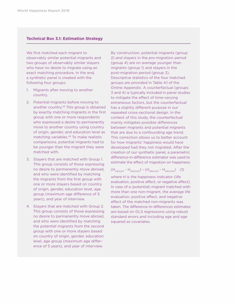
World Happiness Report 2018
Technical Box 3.1: Estimation Strategy
We first matched each migrant to
observably similar potential migrants and
two groups of observably similar stayers
who have no desire to migrate using an
exact matching procedure. In the end,
a synthetic panel is created with the
following four groups:
1. Migrants after moving to another
country.
2. Potential migrants before moving to
another country.48 This group is obtained
by exactly matching migrants in the first
group with one or more respondents
who expressed a desire to permanently
move to another country using country
of origin, gender, and education level as
matching variables.49 To make realistic
comparisons, potential migrants had to
be younger than the migrant they were
matched with.
3. Stayers that are matched with Group 1.
This group consists of those expressing
no desire to permanently move abroad,
and who were identified by matching
the migrants from the first group with
one or more stayers based on country
of origin, gender, education level, age
group (maximum age difference of 5
years), and year of interview.
4. Stayers that are matched with Group 2.
This group consists of those expressing
no desire to permanently move abroad,
and who were identified by matching
the potential migrants from the second
group with one or more stayers based
on country of origin, gender, education
level, age group (maximum age differ-
ence of 5 years), and year of interview.
By construction, potential migrants (group
2) and stayers in the pre-migration period
(group 4) are on average younger than
migrants (group 1) and stayers in the
post-migration period (group 3).
Descriptive statistics of the four matched
groups are provided in Table A1 of the
Online Appendix. A counterfactual (groups
3 and 4) is typically included in panel studies
to mitigate the effect of time-varying
extraneous factors, but the counterfactual
has a slightly different purpose in our
repeated cross-sectional design. In the
context of this study, the counterfactual
mainly mitigates possible differences
between migrants and potential migrants
that are due to a confounding age trend.
This correction allows us to better account
for how migrants’ happiness would have
developed had they not migrated. After the
creation of our synthetic panel, a parametric
difference-in-difference estimator was used to
estimate the effect of migration on happiness:
(HGROUP1
- HGROUP2
) - (HGROUP3
- HGROUP4
) (1)
where H is the happiness indicator (life
evaluation, positive affect, or negative affect).
In case of a (potential) migrant matched with
more than one non-migrant, the average life
evaluation, positive affect, and negative
affect of the matched non-migrants was
taken. The difference-in-differences estimates
are based on OLS regressions using robust
standard errors and including age and age
squared as covariates.
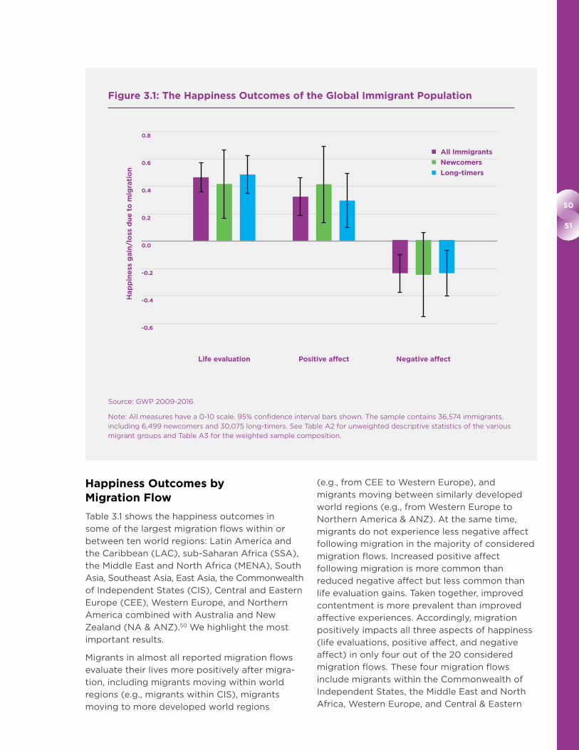
50
51
Happiness Outcomes by Migration Flow
Table 3.1 shows the happiness outcomes in
some of the largest migration flows within or
between ten world regions: Latin America and
the Caribbean (LAC), sub-Saharan Africa (SSA),
the Middle East and North Africa (MENA), South
Asia, Southeast Asia, East Asia, the Commonwealth
of Independent States (CIS), Central and Eastern
Europe (CEE), Western Europe, and Northern
America combined with Australia and New
Zealand (NA & ANZ).50 We highlight the most
important results.
Migrants in almost all reported migration flows
evaluate their lives more positively after migra-
tion, including migrants moving within world
regions (e.g., migrants within CIS), migrants
moving to more developed world regions
(e.g., from CEE to Western Europe), and
migrants moving between similarly developed
world regions (e.g., from Western Europe to
Northern America & ANZ). At the same time,
migrants do not experience less negative affect
following migration in the majority of considered
migration flows. Increased positive affect
following migration is more common than
reduced negative affect but less common than
life evaluation gains. Taken together, improved
contentment is more prevalent than improved
affective experiences. Accordingly, migration
positively impacts all three aspects of happiness
(life evaluations, positive affect, and negative
affect) in only four out of the 20 considered
migration flows. These four migration flows
include migrants within the Commonwealth of
Independent States, the Middle East and North
Africa, Western Europe, and Central & Eastern
Figure 3.1: The Happiness Outcomes of the Global Immigrant Population
Source: GWP 2009-2016.
Note: All measures have a 0-10 scale. 95% confidence interval bars shown. The sample contains 36,574 immigrants, including 6,499 newcomers and 30,075 long-timers. See Table A2 for unweighted descriptive statistics of the various migrant groups and Table A3 for the weighted sample composition.
0.8
0.6
0.4
0.2
0.0
-0.2
-0.4
-0.6
Hap
pin
ess
gain
/lo
ss d
ue
to
mig
rati
on
Life evaluation
All Immigrants
Newcomers
Long-timers
Positive affect Negative affect
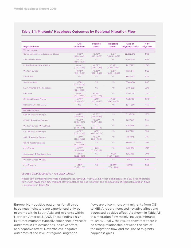
World Happiness Report 2018
Europe. Non-positive outcomes for all three
happiness indicators are experienced only by
migrants within South Asia and migrants within
Northern America & ANZ. These findings high-
light that migrants typically experience divergent
outcomes in life evaluations, positive affect,
and negative affect. Nevertheless, negative
outcomes at the level of regional migration
flows are uncommon; only migrants from CIS
to MENA report increased negative affect and
decreased positive affect. As shown in Table A5,
this migration flow mainly includes migrants
to Israel. Finally, the results show that there is
no strong relationship between the size of
the migration flow and the size of migrants’
happiness gains.
Table 3.1: Migrants’ Happiness Outcomes by Regional Migration Flow
Migration flowLife
evaluationPositive affect
Negative affect
Size of migrant stocka
N of migrants
Within regions
Commonwealth of Independent States +0.39** [0.28 - 0.49]
+0.43** [0.23 - 0.63]
-0.51** [-0.64 - -0.37]
22,092,847 4,176
Sub-Saharan Africa +0.21** [0.06 - 0.35]
NS NS 15,952,589 4,184
Middle East and North Africa +0.44** [0.21 - 0.66]
+0.57** [0.18 - 0.96]
-0.95** [-1.36 - -0.54]
14,273,111 2,563
Western Europe +0.45** [0.31 - 0.60]
+0.36** [0.12 - 0.60]
-0.31** [-0.53 - -0.09]
11,525,545 4,123
South Asia NS NS NS 9,653,943 524
Southeast Asia +1.08* [0.13 - 2.03]
NS NS 7,044,470 607
Latin America & the Caribbean +0.45** [0.24 - 0.66]
NS NS 5,918,332 1,846
East Asia +0.54** [0.23 - 0.84]
+0.85** [0.46 - 1.24]
NS 5,204,219 1,062
Central & Eastern Europe +0.39** [0.26 - 0.52]
+0.51** [0.27 - 0.75]
-0.49** [-0.67 - -0.31]
3,064,126 3,517
Northern America & ANZ NS NS NS 2,245,399 455
Between regions
CEE Western Europe +0.78** [0.58 - 0.97]
+0.50** [0.15 – 0.85]
NS 11,296,274 1,609
MENA Western Europe +0.90** [0.64 - 1.17]
+0.86** [0.37 - 1.35]
NS 9,239,336 655
Western Europe NA&ANZ +0.84** [0.53 - 1.14]
+0.73* [0.14 - 1.32]
NS 6,785,656 1,627
LAC Western Europe +0.36** [0.15 - 0.56]
-0.37* [-0.70 - -0.04]
NS 4,627,262 734
SSA Western Europe +1.44** [1.03 - 1.86]
+0.87** [0.16 - 1.58]
NS 4,111,872 375
CIS Western Europe +0.59** [0.22 – 0.96]
NS NS 4,053,523 396
CIS CEE +0.57** [0.26 - 0.88]
+0.69* [0.10 – 1.28]
NS 1,481,054 1,975
South Asia Southeast Asia +0.80* [0.08 - 1.51]
NS -0.93* [-1.64 - -0.22]
1,219,086 308
Western Europe CEE NS NS NS 768,172 653
CIS MENA +1.11** [0.66 - 1.66]
NS +0.57** [0.14 - 1.00]
461,174 908
Sources: GWP 2009-2016. a UN DESA (2015).51
Notes: 95% confidence intervals in parentheses.* p<0.05, ** p<0.01, NS = not significant at the 5% level. Migration flows with fewer than 300 migrant-stayer matches are not reported. The composition of regional migration flows is presented in Table A5.

52
53
It should be noted that the happiness outcomes
of migrants from a given source region to the
various destination regions are not directly
comparable. For example, the slightly higher
happiness gains among migrants within LAC
compared with Latin American migrants moving
to Western Europe does not imply that those
who moved to Western Europe would have been
better off had they moved within LAC. One
reason is that the considered migration flows
differ in the distribution of source countries.
For example, compared with Argentinians,
relatively more Nicaraguans move within Latin
America than to Western Europe. Another
reason is that migrants in different migration
flows may have different characteristics. For
example, many migrants moving within regions
do not have the financial resources to move to
another world region and certain types of
migrants (e.g., humanitarian migrants) are
admitted in some countries/regions but not
in others. Moreover, the achieved happiness
gains are not indicative of the maximum
possible happiness gain of a certain migration
flow. For instance, most Latin American
migrants in Western Europe live in Spain
and Portugal, but they may have been
happier had they moved to another Western
European country.
In Table 3.2, we present migrants’ happiness
outcomes in selected flows between specific
nations. One general pattern that emerges is the
positive outcomes among United Kingdom (UK)
emigrants who moved to other Anglo-Saxon
countries. Another general pattern is the
non-positive outcomes of Russia-born people
Table 3.2: Migrants’ Happiness Outcomes in Migration Flows Between Specific Nations
Migration flowLife
evaluationPositive affect
Negative affect
N of migrants
United Kingdom Ireland +0.65** [0.48 - 0.81]
+0.72** [0.43 - 1.01]
-0.54** [-0.83 - -0.25]
478
United Kingdom Australia +0.94** [0.76 - 1.11]
NS -0.64** [-0.91 - -0.37]
528
United Kingdom New Zealand +1.11** [0.95 - 1.26]
+0.83** [0.58 - 1.08]
-0.97** [-1.22 - -0.72]
519
Russia Estonia -0.28** [-0.45 - -0.12]
-0.91** [-1.26 - -0.56]
NS 691
Russia Latvia NS NS NS 416
Russia Belarus +0.45** [0.25 - 0.65]
NS -0.33* [-0.64 - -0.01]
385
Russia Kazakhstan +0.28* [0.05 - 0.52]
+0.57* [0.10 - 1.04]
-0.71** [-1.04 - -0.37]
338
Russia Israel +1.55** [1.40 - 1.71]
NS +1.42** [1.15 - 1.69]
580
China Hong Kong +0.16* [0.01 - 0.31]
-0.43** [-0.70 - 0.16]
+0.24* [0.02 - 0.46]
829
Palestinian Territories Jordan +1.63** [1.42 - 1.84]
+1.03** [0.64 - 1.42]
-2.09** [-2.42 - -1.76]
626
Nicaragua Costa Rica +1.48** [1.24 - 1.72]
+0.60** [0.31 - 0.89]
-0.79** [-1.12 - -0.46]
459
France Luxembourg +0.83** [0.66 - 1.00]
+0.67** [0.30 - 1.04]
-1.02** [-1.35 - -0.69]
361
Portugal Luxembourg +1.43** [1.23 - 1.63]
+0.49** [0.08 - 0.90]
-1.05** [-1.42 - -0.68]
352
Albania Greece NS NS NS 355
Serbia Montenegro +0.48** [0.19 - 0.77]
+0.79** [0.29 - 1.27]
NS 309
Ivory Coast Burkina Faso NS -0.90** [-1.37 - -0.43]
NS 310
Source: GWP 2009-2016.
Notes: 95% confidence intervals in parentheses. * p<0.05, ** p<0.01, NS = not significant at the 5% level. Migration flows with fewer than 300 migrant-stayer matches are not reported.

World Happiness Report 2018
who moved to the Baltic states, whereas
Russia-born migrants in some other former
Soviet republics did gain happiness from
migration. A noteworthy finding is that
Russia-born people in Israel evaluate their
lives much more positively after migration but
simultaneously experience adverse outcomes in
terms of affect. These results are in line with the
relatively high life evaluations but relatively low
emotional well-being of Israel’s native population
(Israel ranks 14th out of 156 countries on the
Cantril ladder but 107th out of 156 countries
on net affect in the period 2005-2011).52 The
happiness outcomes of Russia-born migrants
in Israel mainly drive the results reported in
Table 3.1 for migrants from CIS to MENA.
In Chapter 2 of this World Happiness Report,
it was shown that the happiness of immigrants
does not differ much from that of the native-
born population. This finding suggests that the
happiness of immigrants depends first and
foremost on their conditions in the host country
and relatively less on their former lives in their
countries of origin or innate cultural differences
in happiness. We further test to what extent the
happiness levels of migrants converge towards
the average happiness level in the destination
Figure 3.2: The Relationship Between Migrants’ Happiness Gains and the Corresponding Origin-Destination Happiness Differential
Source: GWP 2009-2016.
Notes: The interpretation of these graphs can be exemplified using the upper right data point in the “life evaluations” panel. This data point represents migrants from sub-Saharan Africa to Western Europe, and shows that these migrants evaluate their lives 1.44 higher due to migration (as presented on the X-axis) while the corresponding difference in life evaluations between the native populations of their host- and origin countries is 2.29 (as presented on the Y-axis). The origin-destination differential is weighted by the size of bilateral migration flows within these world regions to ensure accurate comparisons. Detailed information is presented in Table A6.

54
55
country by comparing a migrant’s happiness
gain with the happiness differential between the
migrant’s origin and destination country. This
origin-destination happiness differential is
calculated by subtracting the average happiness
level in the country of origin from that of the
destination country’s native-born population.
Figure 3.2 shows three scatter plots—one for
each happiness indicator—of migrants’
happiness gains/losses due to migration (as
presented on the X-axis) and the corresponding
origin-destination happiness differentials (as
presented on the Y-axis). The data points
represent the 20 regional migration flows
considered in Table 3.1. Migrants’ happiness levels
tend to become more similar to those of people
in their destination country when there is a high
positive correlation between migrants’ happiness
gains and the destination-origin happiness
differential, i.e., when the points are closer to
the 45-degree lines in each panel. Indeed, we
find a strong positive correlation between the
life evaluation gains of migrants and the life
evaluation differentials between their origin and
destination countries (r=0.80). The correlations
for positive affect (r=0.48) and negative affect
(r=0.35) are also positive but more moderate.
These results provide further evidence that the
happiness of migrants converges substantially
— though not entirely — towards the average
happiness level in the host country, particularly in
terms of life evaluations. Migrant happiness thus
strongly depends on the host country environment.
The refugee population requires special attention
because refugees are exceptionally vulnerable and
are the only migrant group for which migration is
largely involuntary. An analysis focusing on the
happiness of refugees is presented in Box 3.2.
Box 3.2: Refugee Happiness
As refugees cannot be identified in the GWP,
we use migrant data from the German
Socio-Economic Panel (SOEP) to empirically
assess how the happiness of refugees
develops with their length of stay in Germany
and how happy refugees are relative to
“voluntary” immigrants in Germany
(job-seekers, expats with job offers, co-moving
family members, etc.). We focus here on the
cognitive dimension of happiness using a life
satisfaction question.53 Our sample contains
607 refugees and 4,607 voluntary migrants.
Column 1 of Table 3.3 shows that refugees
are significantly less satisfied with life than
voluntary migrants and that the general
immigrant population experiences decreasing
life satisfaction with their length of stay in
Germany. Column 2 shows that the non-
positive relationship between life satisfaction
and the time since migration holds both for
refugees and voluntary immigrants in
Germany.54 These findings concur with the
previously shown global pattern that
immigrants in general do not become
happier with their length of stay in the host
country. Taken together, refugees are unable
to close the happiness gap with other
immigrants (and natives), at least in Germany.
However, refugees’ non-improving happiness
with their length of stay does not necessarily
imply that they do not become happier by
migrating; refugees may obtain a substantial
immediate happiness gain upon arrival in
Germany due to their improved safety,
freedom, and so forth. A more detailed
analysis, reported in Table A8, shows that
refugees are significantly less happy than all
specific subgroups of voluntary immigrants
(job-seekers, co-moving family members,
and so forth).

World Happiness Report 2018
The Happiness Outcomes of Families Left Behind
We estimate the happiness consequences
of having a household member abroad by
comparing the happiness of individuals with
and without a household member abroad. For
this purpose, we use global GWP data spanning
the period 2007-2011. To account for the
non-random selection of households into
migration, we employ exact matching and
compare only individuals with the same gender
and education level, who are from the same
country of residence and age group (maximum
age difference of 5 years), and who live in a
similar type of location (rural vs. urban).55
In a first model, we estimate how having one or
multiple household members living abroad for
under five years affects the happiness of left-
behind household members across 144 countries.
We do not have information on the exact
relationship between the migrant and left-behind
household member and the migrant’s motive for
migration. However, it is conceivable that one of
the most common reasons for moving abroad
without other household members is to improve
the household’s living standard by working
abroad and sending back remittances. This
group of migrant workers is characterized by
great diversity, ranging from female nurses from
the Philippines to male construction workers
from Latin America. The household member
abroad can, however, also be another family
member (e.g., a child or sibling) or move for
different reasons (e.g., for study purposes).
Household members left behind are likely to be
Table 3.3: OLS Regression: Life Satisfaction of Refugees and Voluntary Migrants by Length of Stay
Dependent variable: Life satisfaction (1) (2)
Type of migrant
Refugees Ref. Ref.
Voluntary migrants 0.39** 0.48**
(0.08) (0.16)
Years since migration -0.01** -0.00
(0.00) (0.01)
Years since migration*type of migrant
Refugees Ref.
Voluntary migrants -0.01
(0.01)
Age -0.02* -0.02*
(0.01) (0.01)
Age2/100 0.01 0.01
(0.01) (0.01)
Female 0.04 0.04
(0.05) (0.05)
Observations 5,214 5,214
R2 0.02 0.02
Sources: IAB-SOEP Migration samples M1 (2013-2015) and M2 (2015).
Notes: Regression coefficients are displayed with robust standard errors in parentheses. * p<0.05, ** p<0.01. Refugees moved to Germany on average 13 years ago; 48% of these refugees come from MENA (primarily Iraq, Syria, Afghanistan, and Turkey), 26% from the former Yugoslavia, 14% from the former Soviet Union, and 12% from other world regions. See Table A7 for detailed sample descriptives. For the M1 sample, the average life satisfaction over the years 2013–2015 was taken.

56
57
the migrant’s spouse, children, parents, siblings,
or other extended family members. The results,
presented in the upper left panel of Figure 3.3,
show that individuals with a household member
abroad typically evaluate their lives more
positively and experience more positive affect
than their counterparts without a relative abroad.
However, they also experience more negative
affect. A plausible explanation for these mixed
happiness outcomes is that the family’s often
significant economic gain from migration is more
strongly related to cognitive assessments of
quality of life (life evaluations) than affective
experiences,56 and those left behind may
Figure 3.3: The Impact of Migration on the Happiness of Household Members Left Behind
Sources: a Worldwide GWP 2007-2011 data. b GWP 2009 data covering all countries of the former Soviet Union, most Latin American countries, and some Caribbean countries. c GWP 2007 data covering most Latin American countries and the Dominican Republic.
Note: 95% confidence interval bars shown.
Life evaluation Positive affect Negative affect
Hap
pin
ess
gain
/lo
ss
Individuals receiving remittances from relatives abroad (N=1,049)c
Individuals with a household member living permanently abroad (N=1,259)b
0.6
0.5
0.4
0.3
0.2
0.1
0.0
-0.1
-0.2
-0.3
All individuals with a household member abroad (N=44,347)a
Hap
pin
ess
gain
/lo
ss
Individuals with a household member abroad for temporary work (N=2,898)b
0.6
0.5
0.4
0.3
0.2
0.1
0.0
-0.1
-0.2
-0.3
World Happiness Report 2018
often suffer emotionally because they may
experience increased sadness from being
separated from the migrated household member
and increased worry from communicating
infrequently with the family member and
being unable to share responsibilities such
as child nurturing.57
The two right panels of Figure 3.3 present the
outcomes of household members left behind by
household members who specifically moved
abroad for temporary work or permanent
residence, respectively. The analysis sample is
limited to countries in Latin America and the
Caribbean and countries of the former Soviet
Union. Household members left behind by
migrants moving for temporary work or to
permanently live abroad evaluate their lives
more positively than their counterparts without
a household member abroad. However, they do
not benefit from migration in terms of emotional
well-being; most notably, individuals with a
household member abroad for temporary work
experience increased negative affect following
migration. Similarly, as shown in the lower left
panel, Latin Americans who receive remittances
from relatives abroad evaluate their lives more
positively and experience more positive affect
but they do not experience less negative affect
compared with non-migrant households.
Taken together, the results reported in Figure 3.3
suggest that migration generally improves the
perceived quality of life of household members
back home but not necessarily their emotional
well-being. Particularly interesting is that having
a household member abroad generally does not
reduce—and often even increases—negative
affect experiences among the family back home.
Hence, migration often requires trade-offs
between different aspects of happiness for
people staying behind.
In Table 3.4, we present the impact of migration
on left-behind household members for selected
migration flows within or between world regions.
The analysis sample contains all individuals with
a household member abroad, i.e., the sample as
in the upper left panel of Figure 3.3. There is
considerable heterogeneity in outcomes be-
tween migration flows. The benefits in terms of
life evaluations and positive affect are particularly
large for individuals in the developing world
who have a household member living in Western
Europe, Northern America, Australia, or New
Zealand. It is plausible that benefits are largest in
these migration flows given that the large wage
gaps between these origin and destination
regions allow for high remittances. However, in
some cases, benefits are also present among
families left behind in other types of migration
flows, such as migrants moving within the
Commonwealth of Independent States. In 8 out
of 21 migration flows, non-positive outcomes are
experienced for all three aspects of happiness.
For example, household members left behind by
migrants within MENA experience increased
negative affect and no improvements in life
evaluations or positive affect. Interestingly,
there are no migration flows in which migration
reduced negative affect experiences among
families back home, which highlights the
prevalence of a non-positive impact of migration
on the negative affect experiences of those
staying behind. Outcomes between bilateral
migration flows are presented in Table 3.5.
Robustness Checks and Limitations
Some possible validity threats cannot be fully
addressed in our cross-sectional study, which
is typical of empirical literature estimating the
impact of migration on migrants and families
left behind.58 A first concern relates to migrant
selectivity. In our analysis of migrant outcomes,
we mitigated possible selection bias in terms of
demographics, skills, ability, personality, and
other characteristics to the extent possible by
introducing potential migrants as a comparison
group and by comparing migrants only to
demographically similar stayers. Nevertheless,
unobserved migrant-stayer differences in per-
sonal characteristics that affect happiness could
remain present and may bias our results to some
extent. To alleviate this concern, we conducted a
robustness check in which potential migrants
were replaced by a smaller sample of migrants
with concrete plans to migrate within a year. The
pre-migration characteristics of our migrant
sample may be more similar to those of people
with concrete migration plans than to those of
people expressing only a willingness to migrate.
A potential limitation of using migrants with
concrete migration plans as a comparison group
is that their anticipated migration may have
affected their happiness. The results using this

58
59
alternative comparison group are reported in
Figure A1 and are consistent with our main finding
that migrants are generally better off after migra-
tion on all three happiness indicators. However,
compared with our main results, migration has a
somewhat weaker impact on positive affect and
a stronger impact on negative affect.
Second, temporary migrants live for a shorter
period in the host country compared with
permanent migrants and thus have a smaller
chance of being sampled in the host country.
Therefore, temporary migrants are likely to be
under-represented in our sample. This may bias
the results if returnees achieve relatively better
or worse happiness outcomes in the host country
than permanent migrants. However, return
migration is in many cases not primarily driven
by the success of the migration experience
(e.g., for refugees returning home), whereas in
other cases return migration resulting from a
disappointing migration experience is to some
extent counterbalanced by return migration
resulting from having successfully achieved one’s
migration goals.59 Nevertheless, non-causal
evidence shows that returnees tend to be less
happy than stayers in the home country and
non-returned migrants, which may be either
because return migrants were already relatively
unhappy before moving abroad or because
migrants with disappointing migration outcomes
are more inclined to return home.60 Based on the
current evidence, we cannot provide a reliable
estimate of the extent and direction of the bias
resulting from the underrepresentation of
temporary migrants.
Third, our migrant sample excludes some migrant
groups. Migrants in Gulf Cooperation Council
countries and sparsely populated countries and
island states are excluded, representing altogether
less than 8% of the world’s migrant population.61
Aside from the exclusion of these groups, the
analysis sample was made representative, to the
extent possible, of each destination country’s
immigrant stock size by virtue of a weighting
adjustment. By contrast, the sample is not fully
representative of the migrant populations within
host countries, since the GWP is not specifically
designed to study migrants. The analysis sample
may particularly under-represent undocumented
migrants and excludes migrants in refugee
camps, migrant children, and migrants who do
not speak the host country’s most common
languages. The latter two groups are excluded
because GWP respondents are aged 15+ and
interviews are only held in each country’s most
common languages, respectively. Initial evidence
suggests that proficiency in the host country
language may improve immigrant happiness,62
whereas there is no specific research available
on the happiness gains of the other excluded
immigrant groups.63 The exclusion of these
groups must be taken into account when
interpreting the results.
Fourth, interviews are conducted over the
phone in developed countries, including Western
Europe, Northern America & ANZ, and some
East-Asian countries, but face-to-face in most of
the developing world, including CIS, sub-Saharan
Africa, South Asia, and much of Latin America,
Southeast Asia, and MENA (see Table A11).
Approximately 25% of the face-to-face interviews
in our migrant sample were computer-assisted
(CAPI). The lack of within-country variance in
survey mode in a given year constrained us from
statistically correcting for possible survey mode
bias in our main analysis. In Table A12, we show
that life evaluations and self-reported negative
and positive affect are not significantly affected
by survey mode (phone, face-to-face without CAPI, or face-to-face with CAPI), with one
exception. A person interviewed by phone
reports 0.60 points higher negative affect on
a 0-10 scale than if s/he had been interviewed
face-to-face without CAPI.64 Particularly for
negative affect, then, survey mode differences
may somewhat bias outcome estimations for
migration flows between developing and
developed regions. Nevertheless, this bias will
have a negligible impact on the average global
happiness outcome from migration because
migration flows in opposite directions counter-
balance this bias to some extent, and many
migrants move between countries with the
same survey mode.
We ask readers to take these limitations into
account when interpreting our results.
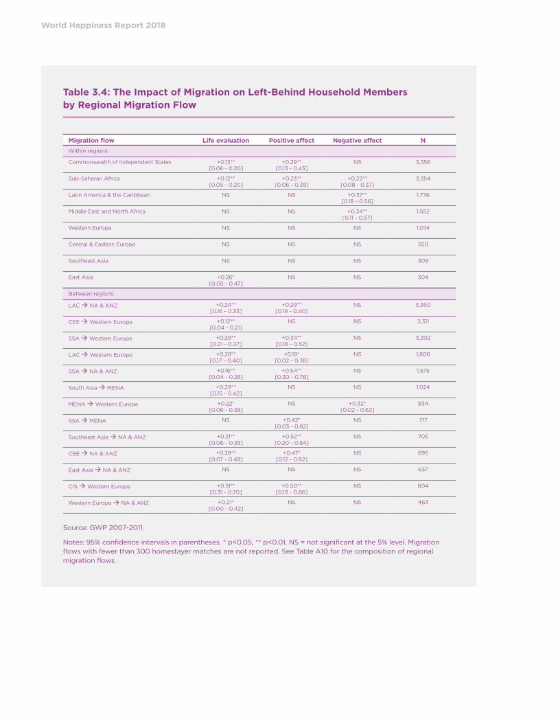
World Happiness Report 2018
Table 3.4: The Impact of Migration on Left-Behind Household Members by Regional Migration Flow
Migration flow Life evaluation Positive affect Negative affect N
Within regions:
Commonwealth of Independent States +0.13** [0.06 - 0.20]
+0.29** [0.13 - 0.45]
NS 3,356
Sub-Saharan Africa +0.12** [0.05 - 0.20]
+0.23** [0.06 - 0.39]
+0.23** [0.08 - 0.37]
3,354
Latin America & the Caribbean NS NS +0.37** [0.18 - 0.56]
1,776
Middle East and North Africa NS NS +0.34** [0.11 - 0.57]
1,552
Western Europe NS NS NS 1,074
Central & Eastern Europe NS NS NS 550
Southeast Asia NS NS NS 309
East Asia +0.26* [0.05 - 0.47]
NS NS 304
Between regions:
LAC NA & ANZ +0.24** [0.16 - 0.33]
+0.29** [0.19 - 0.40]
NS 3,360
CEE Western Europe +0.12** [0.04 - 0.21]
NS NS 3,311
SSA Western Europe +0.29** [0.21 - 0.37]
+0.34** [0.16 - 0.52]
NS 3,202
LAC Western Europe +0.28** [0.17 - 0.40]
+0.19* [0.02 - 0.36]
NS 1,806
SSA NA & ANZ +0.16** [0.04 - 0.28]
+0.54** [0.30 - 0.78]
NS 1,575
South Asia MENA +0.29** [0.15 - 0.42]
NS NS 1,024
MENA Western Europe +0.22* [0.06 - 0.38]
NS +0.32* [0.02 - 0.62]
834
SSA MENA NS +0.42* [0.03 - 0.82]
NS 717
Southeast Asia NA & ANZ +0.21** [0.06 - 0.35]
+0.52** [0.20 - 0.84]
NS 705
CEE NA & ANZ +0.28** [0.07 - 0.49]
+0.47* [0.12 - 0.82]
NS 695
East Asia NA & ANZ NS NS NS 637
CIS Western Europe +0.51** [0.31 - 0.70]
+0.50** [0.13 - 0.86]
NS 604
Western Europe NA & ANZ +0.21* [0.00 - 0.42]
NS NS 463
Source: GWP 2007-2011.
Notes: 95% confidence intervals in parentheses. * p<0.05, ** p<0.01. NS = not significant at the 5% level. Migration flows with fewer than 300 homestayer matches are not reported. See Table A10 for the composition of regional migration flows.

60
61
Conclusions and Implications
Using Gallup World Poll data, this chapter sheds
light on the happiness consequences of migration
for international migrants and families left behind
across the globe. Three types of happiness
outcomes were considered: life evaluations,
positive affect (experiences of enjoyment,
happiness, and laughter), and negative affect
(experiences of worry, sadness, and anger).
By comparing migrants to matched potential
migrants and stayers without migration plans, we
estimate that migrants across the globe evaluate
the quality of their lives on average 9% higher
following migration. They also experience ap-
proximately 5% more positive affect and 7% less
negative affect due to migration. Accordingly,
the happiness levels of migrants converge
substantially towards the average happiness level
in the host country, particularly in terms of life
evaluations. Most of these happiness gains are
already experienced within the first five years
after migration given that the happiness of
international migrants generally does not further
improve following those first five years.
A happiness gain in at least one of the three
happiness indicators is not only the dominant
outcome among migrants moving to more
developed world regions (e.g., from Central and
Eastern Europe to Western Europe) but also
among migrants moving between similarly
developed world regions (e.g., from Western
Europe to Northern America & ANZ), or within
world regions (e.g., migrants within Latin America
and the Caribbean). Notable groups that have
not become happier, in some or all aspects of
happiness, by migrating include migrants within
South Asia, migrants within Northern America &
ANZ, Albanian migrants in Greece, migrants from
the Ivory Coast in Burkina Faso, and Russian-
born migrants in the Baltic states. These findings
imply that despite the happiness gains achieved
Table 3.5: The Impact of Migration on Left-Behind Household Members in Migration Flows Between Specific Nations
Migration flow Life evaluation Positive affect Negative affect N
Tajikistan Russia +0.22* [0.09 – 0.35]
NS NS 918
Kyrgyzstan Russia NS +0.61** [0.27 - 0.94]
NS 642
Armenia Russia +0.48** [0.27 - 0.68]
NS NS 360
Moldova Russia NS NS NS 323
Honduras United States NS NS NS 493
El Salvador United States NS NS NS 466
Guatemala United States +0.23* [0.00 - 0.26]
NS NS 361
Paraguay Argentina NS -0.34* [-0.67 - -0.02]
+0.49** [0.12 - 0.84]
406
Zimbabwe South Africa NS +0.65* [0.10 - 1.19]
NS 385
Bolivia Spain +0.34* [0.05 - 0.62]
+0.60** [0.23 - 0.97]
NS 324
East Asia NA & ANZ NS NS NS 637
CIS Western Europe +0.51** [0.31 - 0.70]
+0.50** [0.13 - 0.86]
NS 604
Western Europe NA & ANZ +0.21* [0.00 - 0.42]
NS NS 463
Source: GWP 2007-2011.
Notes: 95% confidence intervals in parentheses * p<0.05, ** p<0.01, NS = not significant at the 5% level. Migration flows with fewer than 300 home stayer matches are not reported.
World Happiness Report 2018
by a majority of migrants, there is a considerable
group of international migrants who do not
become happier from migration.
Migration has a mixed impact on the happiness
of possible household members who stay behind
in the country of origin. Household members left
behind generally evaluate their lives more posi-
tively after the migration of a household mem-
ber. A plausible reason for this positive impact is
the receipt of remittances. However, they also
experience on average more—or at least no
reduced—negative affect. This suggests that the
disadvantages of migration, such as impaired
emotional support, are more related to affect,
while the benefits of migration, such as an
increased living standard, are more related to life
evaluations. Not surprisingly, the greatest bene-
fits are experienced by families in the developing
world who have a household member living in a
developed country.
Our findings suggest that it is likely that a
portion of migrants who did not gain happiness
from migration sacrificed happiness for the
benefit of their family back home. However,
for many other migrants who are not happier
after migration, this reason may not apply. For
instance, in some migration flows in which
non-positive outcomes are common, such as
migration flows between developed countries,
the entire household typically moves or the
migrant does not specifically move to improve
the lives of family members back home. One
question that thus requires attention is why
some migrants voluntarily move abroad if it
benefited neither themselves nor their families
back home. These non-positive happiness
outcomes cannot be justified by the argument
that one invests in one’s own long-term
happiness or the happiness of one’s children
because we do not find that happiness increases
with the migrant’s length of stay, while existing
literature shows that the second generation is
not happier than first-generation migrants.65
Migrants may trade off happiness for other goals,
such as economic security, freedom, safety,
and health. However, in most cases, positive
outcomes in these other domains go together
with greater happiness. For example, greater
happiness often accompanies greater health and
safety. A more worrisome but oft-mentioned
potential cause of negative outcomes is migrants’
excessive expectations about their future happiness
in the destination country, which originate from
inaccurate perceptions about what determines
their happiness and inaccurate or incomplete
information about the destination country.66
The opposite question also requires attention:
Considering the substantial happiness gains
experienced by most international migrants, why
don’t more than the current 250 million people
(3.3% of the world population) live in a country
other than where they were born? It seems likely
that more people could benefit from migration,
given the large happiness differences between
countries and the benefits for the current
international migrant population. Several
reasons may apply. First, many people are
restricted from migration by personal
constraints, such as financial, health, or family
constraints. Second, many people cannot move
to their preferred destination countries because
of those countries’ restrictive admission
policies.67 Third, many people are locally
oriented and moving abroad is simply not a
salient pathway in people’s long-term orientation
toward improving their lives. Finally, according
to prospect theory, the human tendency for
risk- and loss aversion may cause people to stay
in their home countries given that many people
face great uncertainty about the outcomes of
migration as they have little knowledge about
life abroad.68
In sum, international migration is, for many
people, a powerful instrument to improve their
lives given that the majority of migrants and
families back home benefit considerably from
migration. Nevertheless, not all migrants and
families left behind gain happiness from
migration, and the happiness of migrants does
not increase over time as they acclimatize to
their new country. Therefore, there is still much
to be done, and much to be learned, to ensure
lasting benefits for migrants and their families.

62
63
Endnotes
1 See, e.g., IOM (2015) on migrant exploitation, Portes and Zhou (1993) on unsuccessful socio-economic assimilation, and Dreby (2010) on homesickness.
2 Esipova et al. (2017).
3 United Nations (2015).
4 Diener et al. (1999).
5 UNHCR (2017).
6 Ottonelli and Torresi (2013).
7 Benjamin et al. (2014).
8 For an overview of basic human needs, see Maslow’s hierarchy of needs (1943).
9 Nikolova and Graham (2015), Zuccotti et al. (2017).
10 Morosanu (2013).
11 Berry (2006).
12 Frey and Stutzer (2014).
13 Mahler (1995), Sayad (2004), Mai (2005).
14 Schkade and Kahneman (1998), Gilbert (2006).
15 Frey and Stutzer (2014).
16 See particularly the “Easterlin paradox” (Easterlin 1974).
17 Bartram (2013a), Olgiati et al. (2013), Hendriks and Bartram (2016).
18 For exceptions, see Mähönen et al. (2013), Nikolova and Graham (2015), and Stillman et al. (2015).
19 See, e.g., IOM (2013).
20 Boneva and Frieze (2001), Jaeger et al. (2010), McKenzie et al. (2010).
21 Graham and Markowitz (2011), Cai et al. (2014).
22 See Hendriks (2015) for a review and Nikolova and Graham (2015) and IOM (2013) for studies using GWP data.
23 Stillman et al. (2015).
24 Bartram (2013a).
25 Knight and Gunatilaka (2010).
26 Hendriks et al. (2018).
27 Ratha et al. (2016).
28 Stark and Bloom (1985).
29 See Antman (2013) for a review of how migration affects various well-being outcomes of children, spouses, and parents who remain in the country of origin.
30 Dreby (2010), Abrego (2014).
31 Joarder et al. (2017).
32 Borraz et al. (2010).
33 Jones (2014; 2015).
34 Cárdenas et al. (2009).
35 Gibson et al. (2011), Böhme et al. (2015), Nobles et al. (2015).
36 See Stillman et al. (2015) for a rare study examining migrants’ affective happiness outcomes.
37 First-generation immigrants are those who are not born in their country of residence. Because of data limitations,
immigrants’ native-born children (the second generation) and later generations are beyond the scope of this chapter. Our migrant sample differs from that of Chapter 2 of this World Happiness Report because an important variable for estimating the consequences of migration—country of birth—is not available before 2009. Migrants originating from countries that are not covered by the GWP— predominantly sparsely populated countries and island states—are excluded from analysis because they could not be matched to stayers. Immigrants in Gulf Cooperation Council (GCC) countries are excluded because these countries lack sufficiently representative immigrant samples.
38 Our empirical strategy builds on the work of IOM (2013) and Nikolova and Graham (2015) and is broadly in line with the empirical strategy used by Nikolova and Graham to explore the happiness consequences of migration for migrants from transition countries. For a more general discussion of this methodology, see Blundell and Costa Dias (2000).
39 Van Dalen and Henkens (2013), Creighton (2013), Docquier et al. (2014).
40 Cantril (1965).
41 To be consistent with the Cantril-ladder-of-life measure, both affect indexes were re-scaled to range from 0 to 10.
42 Kahneman and Deaton (2010).
43 The percentage of the happiness gain is calculated by first solving equation 1 (using the sample means of groups 2-4) to find the sample mean of group 1 for which the happiness gain would be zero and subsequently calculating the absolute happiness gain as a percentage of that sample mean.
44 Our results are very similar when we would only compare migrants to potential migrants (groups 1 and 2), i.e., when we would exclude the counterfactual (groups 3 and 4). Specifically, we find a life evaluation gain of 0.49 points, a positive affect gain of 0.37 points, and a decrease in negative affect of 0.29 for the total immigrant sample.
45 In the main analysis, the reported happiness gains for newcomers and long-timers are based on the same weighting criteria (the migrant stock by destination country) to ensure that our assessment of the short- and long-term impacts of migration is not driven by a different distribution of newcomers and long-timers over destination countries. We additionally calculated the happiness gains for “newcomers” using an alternative weighting variable that is more representative for countries’ migration inflows in recent years. This self-created weighting variable is based on each country’s migrant inflow in the period 2005-2010 as estimated by Abel and Sander (2014). When applying this alternative weighting variable, newcomers report 0.41 higher life evaluations after migration (p<.01), Newcomers also report 0.22 more positive affect and 0.08 less negative affect but these gains are not statistically significant.
46 Given our cross-sectional data, possible cohort effects may affect the relative happiness gains of newcomers versus long-timers. However, Hendriks et al. (2018) did not find evidence for cohort effects among immigrants in Western Europe, and Stillman et al. (2015) found no improvement in happiness in the first years after migration using panel data. Hence, it is unlikely that cohort effects drive migrants’ non-improving happiness with their length of stay.
47 See e,g., Safi (2010).
48 The following question was used to identify potential migrants: “Ideally, if you had the opportunity, would you like to move permanently to another country, or would you prefer to continue living in this country?”
49 While education is not independent of migration, we included it to match migrants only to stayers with similar ability, intelligence, and skills.
50 See Table A4 for the regional classification of countries.
51 Underestimation of migration flows to non-developed regions (e.g., sub-Saharan Africa) is likely, as considerable migration flows may go unreported because of the more limited and less reliable collection of data in those regions.
52 Helliwell and Wang (2012).
53 The life satisfaction question is formulated as follows: “How satisfied are you with your life, all things considered?”, with a numerical response scale ranging from 0 (completely dissatisfied) to 10 (completely satisfied).
54 We found no evidence of a non-linear relationship between length of stay and life satisfaction, i.e., the quadratic term for years since migration did not enter significantly into our models and is therefore excluded from our models.
55 Sample descriptives are reported in Table A9. While immigrants in GCC countries were excluded in previous analyses, the analysis samples in this section include families left behind by immigrants in GCC countries. The analyses in this section are based on unweighted data because there are no global data available on the number of left-behind migrant households by origin country or migration flow.
56 Kahneman and Deaton (2010).
57 Nobles et al. (2015), Abrego (2014).
58 For example, the literature on migrants’ income gains from migration emphasizes that cross-sectional studies have limited leverage in estimating the benefits of migration because self-selection biases cannot be fully eliminated (e.g., Borjas 1987, McKenzie et al. 2010).
59 De Haas et al. (2015), Esipova and Pugliese (2012).
60 Bartram (2013b), Nikolova and Graham (2015).
61 UN DESA (2015).
62 Angelini et al. (2015).
63 Undocumented migrants and immigrants in refugee camps often face exploitation, discrimination, limited freedom and safety, and other negative circumstances. They may nevertheless have obtained considerable happiness gains because they move away from possibly even more deprived conditions in their home countries; many of these migrants were forced to move because they could not meet their basic subsistence needs back home.
64 Our results differ from Dolan and Kavetsos’ (2016) finding that people report higher happiness over the phone than via CAPI. This may be because their study uses different happiness measures, a different sample (a UK sample), or a different interview procedure.
65 Safi (2010).
66 Schkade and Kahneman (1998), Knight and Gunatilaka (2010), Bartram (2013a), Olgiati et al. (2013).
67 Recent studies in Europe, however, show that if anything, immigrant influxes tend to slightly improve the happiness of the host countries’ native populations, at least in Europe (Betz and Simpson 2013; Akay et al. 2014).
68 Morrison and Clark (2016).
World Happiness Report 2018

64
65
References
Abel, G. J., & Sander, N. (2014). Quantifying global international migration flows. Science, 343(6178), 1520-1522.
Abrego, L. (2014). Sacrificing families: Navigating laws, labor, and love across borders. Stanford University Press.
Akay, A., Constant, A., & Giulietti, C. (2014). The impact of immigration on the well-being of natives. Journal of Economic Behavior & Organization, 103, 72-92.
Angelini, V., Casi, L., & Corazzini, L. (2015). Life satisfaction of immigrants: Does cultural assimilation matter?. Journal of Population Economics, 28(3), 817-844.
Antman, F. M. (2013), The Impact of Migration on Family Left Behind, in A. F. Constant and K. F. Zimmermann (eds.), International Handbook on the Economics of Migration, Edward Elgar, Northampton, MA, 293–308.
Bartram, D. (2013a). Happiness and ‘economic migration’: A comparison of eastern European migrants and stayers. Migration Studies, 1(2), 156-175.
Bartram, D. (2013b). Migration, return, and happiness in Romania. European Societies, 15(3), 408-422.
Benjamin, D.J., Heffetz, O., Kimball, M.S., & Rees-Jones, A. (2014). Can marginal rates of substitution be inferred from happiness data? Evidence from residency choices. The American Economic Review, 104(11), 3498-3528.
Berry, J.W. (2006). Acculturative stress. In P.T.P. Wong & L.C.J. Wong, Handbook of multicultural perspectives on stress and coping (pp. 287–298). Dallas, TX: Spring.
Betz, W. & Simpson, N.B. (2013). The effects of international migration on the well-being of native populations in Europe. IZA Journal of Migration, 2(12), 1-21.
Blundell, R., & Costa Dias, M. (2000). Evaluation methods for non-experimental data. Fiscal studies, 21(4), 427-468.
Böhme, M. H., Persian, R., & Stöhr, T. (2015). Alone but better off? Adult child migration and health of elderly parents in Moldova. Journal of Health Economics, 39, 211-227.
Boneva, B.S. & Frieze, I.H. (2001). Toward a concept of a migrant personality. Journal of Social Issues, 57(3), 477-491.
Borjas G. J. (1987). Self selection and the earnings of immigrants. American Economic Review 77(4): 531–553.
Borraz, F., Pozo, S. & Rossi, M. (2010). And what about the family back home? International migration and happiness in Cuenca, Ecuador. Journal of Business Strategies, 27(1), 7-27.
Brücker, H., Kroh, M., Bartsch, S., Goebel, J., Kühne, S., Liebau, E., ... & Schupp, J. (2014). The new IAB-SOEP Migration Sample: an introduction into the methodology and the contents (No. 216). SOEP Survey Papers.
Cai, R., Esipova, N., Oppenheimer, M., & Feng, S. (2014). International migration desires related to subjective well-being. IZA Journal of Migration, 3(1), 1-20.
Cantril, H. (1965). The pattern of human concerns. New Brunswick, NJ: Rutgers University Press.
Cárdenas, M., Di Maro, V., & Sorkin, I. (2009). Migration and life satisfaction: evidence from Latin America. Journal of Business Strategies, 26(1), 9-33.
Creighton, M. J. (2013). The role of aspirations in domestic and international migration. The Social Science Journal, 50(1), 79-88.
De Haas, H., Fokkema, T., & Fihri, M. F. (2015). Return migration as failure or success?. Journal of International Migration and Integration, 16(2), 415-429.
Diener, E., Suh, E.M., Lucas, R.E., & Smith, H.L. (1999). Subjective well-being: Three decades of progress. Psychological Bulletin, 125(2), 276–302.
Docquier, F., Peri, G., & Ruyssen, I. (2014). The cross-country determinants of potential and actual migration. International Migration Review, 48(s1): S37–S99.
Dolan, P., & Kavetsos, G. (2016). Happy talk: Mode of adminis-tration effects on subjective well-being. Journal of Happiness Studies, 17(3), 1273-1291.
Dreby, J. (2010) Divided by borders: Mexican migrants and their children, Berkeley: University of California Press.
Easterlin, R.A. (1974). Does economic growth improve the human lot? Some empirical evidence, in Nations and households in economic growth: Essays in honor of Moses Abramowitz. Paul A. David and Melvin W. Reder, eds. NY: Academic Press, pp. 89-125.
Esipova, N., Ray, J., & Pugliese, A. (2017). Number of Potential Migrants Worldwide Tops 700 Million. Retrieved from http://news.gallup.com/poll/211883/number-potential- migrants-worldwide-tops-700-million.aspx
Esipova, N. & Pugliese, A. (2012). Labor Migration Doesn’t Always Pay Off for FSU Migrants. Retrieved from http://news.gallup.com/poll/159572/labor-migration-doesn-always-pay- off-fsu-migrants.aspx
Frey, B.S. & Stutzer, A. (2014). Economic consequences of mispredicting utility. Journal of Happiness Studies, 15(4), 937-956.
Gibson, J., McKenzie, D., & Stillman, S. (2011). The impacts of international migration on remaining household members: omnibus results from a migration lottery program. Review of Economics and Statistics, 93(4), 1297-1318.
Gilbert, D.T. (2006) Stumbling on happiness, New York, USA: Knopf.
Graham, C. & Markowitz, J. (2011). Aspirations and happiness of potential Latin American immigrants. Journal of Social Research & Policy, 2(2), 9-25.
Helliwell, J. F., & Wang, S. (2012). The state of world happiness. In J. Helliwell, R. Layard, & J. Sachs (Eds.), World happiness report (pp. 10–57). New York: Earth Institute at Columbia University.
Hendriks, M. (2015). The happiness of international migrants: A review of research findings. Migration Studies. 3(3), 343-369.
Hendriks, M. & Bartram, D. (2016). Macro-conditions and immigrants’ happiness: Is moving to a wealthy country all that matters?. Social Science Research, 56, 90-107.
Hendriks, M., Burger, M., & De Vroome, T. (2018). Unsuccessful subjective well-being assimilation among immigrants: The role of shifting reference points and faltering perceptions of the host society. Working paper.
International Organization for Migration (IOM) (2013). World migration report 2013: Migrant well-being and development. Geneva: IOM.
International Organization for Migration (IOM) (2015). The other migrant crisis - Protecting migrant workers against exploitation in the Middle East and North Africa. Geneva: IOM.

Joarder, M. A. M., Harris, M., & Dockery, A. M. (2017). Remittances and happiness of migrants and their home households: Evidence using matched samples. The Journal of Development Studies, 53(3), 422-443.
Jones, R.C. (2014). Migration and family happiness in Bolivia: Does social disintegration negate economic well-being?. International Migration, 52(3), 177-193.
Jones, R. (2015). Migration pessimism and the subjective well-being of migrant households in Mexico. Bulletin of Latin American Research, 34(3), 305-323.
Kahneman, D., & Deaton, A. (2010). High income improves evaluation of life but not emotional well-being. Proceedings of the National Academy of Sciences, 107(38), 16489-16493.
Knight, J. & Gunatilaka, R. (2010). Great expectations? The subjective well-being of rural urban migrants in China. World Development, 38, 113-124.
Mai, N. (2004). Looking for a more modern life: the role of Italian television in the Albanian migration to Italy. Westminster Papers in Communication and Culture, 1(1), 3-22.
Mahler, S.J. (1995). American dreaming: Immigrant life on the margins. Princeton, NJ: Princeton University Press.
Mähönen, T.A., Leinonen, E., & Jasinskaja-Lahti, I. (2013). Met expectations and the wellbeing of diaspora immigrants: A longitudinal study. International Journal of Psychology, 48(3), 324-333.
Maslow, A.H. (1943). A theory of human motivation. Psychological Review, 50(4), 370-396.
McKenzie, D., Stillman, S., & Gibson, J. (2010). How important is selection? Experimental vs. non-experimental measures of the income gains from migration. Journal of the European Economic Association, 8(4), 913-945.
Morrison, P. S., & Clark, W. A. (2016). Loss aversion and duration of residence. Demographic Research, 35, 1079.
Morosanu, L. (2013). Between fragmented ties and ‘soul friendships’: The cross-border social connections of young Romanians in London. Journal of Ethnic and Migration Studies, 39(3), 353-372.
Nikolova, M. & Graham, C. (2015). In transit: The well-being of migrants from transition and post-transition countries. Journal of Economic Behavior & Organization, 112, 164-186.
Nobles, J., Rubalcava, L., & Teruel, G. (2015). After spouses depart: Emotional wellbeing among nonmigrant Mexican mothers. Social Science & Medicine, 132, 236-244.
Olgiati, A., Calvo, R. & Berkman, L. (2013). Are migrants going up a blind alley? Economic migration and life satisfaction around the world: Cross-national evidence from Europe, North America and Australia. Social Indicators Research, 114(2), 383-404.
Ottonelli, V. & Torresi, T. (2013). When is migration voluntary? International Migration Review, 47(4), 783-813.
Portes, A. & Zhou, M. (1993). The new second generation: Segmented assimilation and its variants. The annals of the American academy of political and social science, 530(1), 74-96.
Ratha, D., Eigen-Zucchi, C., & Plaza, S. (2016). Migration and remittances Factbook 2016. World Bank Publications.
Safi, M. (2010). Immigrants’ life satisfaction in Europe: Between assimilation and discrimination. European Sociological Review, 26(2), 159-176.
Sayad, A. (2004). The suffering of the immigrant. Cambridge: Polity Press.
Schkade, D.A. & Kahneman, D. (1998). Does living in California make people happy? A focusing illusion in judgments of life satisfaction. Psychological Science, 9(5), 340-346.
Stark, O. & Bloom, D.E. (1985). The new economics of labor migration. American Economic Review, 173-178.
Stillman, S. Gibson, J., McKenzie, J., & Rohorua, J., (2015). Miserable migrants? Natural experiment evidence on international migration and objective and subjective well-being. World Development, 65, 79-93.
United Nations, Department of Economic and Social Affairs (UN DESA) (2015). Trends in International Migrant Stock: Migrants by Destination and Origin (United Nations database, POP/DB/MIG/Stock/Rev.2015).
United Nations High Commissioner for Refugees (UNHCR) (2017). Global trends: Forced displacement in 2016. Geneva: UNHCR.
Van Dalen, H. P., & Henkens, K. (2013). Explaining emigration intentions and behaviour in the Netherlands, 2005–10. Population Studies, 67(2), 225-241.
Zuccotti, C.V., Ganzeboom, H.B., & Guveli, A. (2017). Has migration been beneficial for migrants and their children? International Migration Review, 51(1), 97-126.
World Happiness Report 2018

66
67Chapter 4
Rural-Urban Migration and Happiness in China
John Knight, Emeritus Professor, Department of Economics, University of Oxford; Emeritus Fellow, St Edmund Hall, Oxford; Academic Director, Oxford Chinese Economy Programme
Ramani Gunatilaka, Director, Centre for Poverty Analysis, Colombo; Research Associate, International Centre for Ethnic Studies, Colombo
In preparing this chapter we have benefited greatly from the advice and comments of John Helliwell, Richard Layard, Martijn Hendriks, Carol Graham and Paul Frijters.

World Happiness Report 2018
1. Introduction
This chapter links the literatures on rural-urban
migration and on subjective well-being in developing
countries and is one of the few to do so. Using
microeconomic analysis (of people and households),
it poses the question: why do rural-urban migrant
households settled in urban China have an
average happiness score lower than that of rural
households? Three basic possibilities of mistaken
expectations are examined: migrants had false
expectations about their future urban conditions,
or about their future urban aspirations, or about
their future selves. Estimations and analyses,
based on a national household survey, indicate
that certain features of migrant conditions make
for unhappiness, and that their high aspirations
in relation to achievement, influenced by their
new reference groups, also make for unhappiness.
Although the possibility that migrants are not
typical cannot be ruled out, it is apparently
difficult for migrants to form unbiased expectations
about life in a new and different world. Since the
ongoing phenomenon of internal rural-urban
migration in developing countries involves many
millions of the world’s poor, it deserves more
attention from researchers and policymakers,
especially on the implications of migration for
subjective well-being.
Migration can be viewed as a decision, taken
independently by myriad rural-dwellers, to better
themselves and their families by moving to where
the jobs and facilities are. It is generally viewed
as a force for good, albeit one that poses many
challenges for society and for the state. There
are two main forms of rural-urban migration. One
is the permanent movement of entire households
to the city or town. The other is the temporary
movement of individual migrant workers, with at
least part of the household remaining in the
village. The choice is influenced by government
policies of encouragement or discouragement
and by the institutions which can impose private
costs and benefits on the workers or their house-
holds. Both forms of rural-urban migration can
take place simultaneously.
Rural-urban migration in developing countries is
the great exodus of our time. Rapid urbanisation
is taking place in Asia, Africa, Latin America and
elsewhere. Table 4.1 shows urbanisation in the
regions of the developing world over the period
1990-2015. In each region there was a sharp rise
in the urban population as a percentage of total
population. The increase in the urban population
of the developing regions as a whole was no less
than 1,535 million. China was outstanding both in
its increase in the urbanisation rate (by 30
percentage points) and in the number of people
becoming urbanised (by 463 million). China
accounted for 30% of the increase in urban
population of the developing world as a whole
over the period.
China’s urbanisation is not the same as its rural-
urban migration. Urbanisation comprises three
elements: reclassification of rural places as urban
places, natural increase of the urban population,
and rural-urban migration. However, China’s
rural-urban migration is likely to have made up
much of the rise in its urban population over this
quarter century.1
The data on migrants in China pose an interesting
and socially important puzzle. Migration theory
usually assumes that rural people migrate in
order to raise their utility, at least in the long run.
Thus, migrants who have made the transition into
urban employment and living are expected to be
happier than they would have been had they
remained at home. Yet our sample of rural-urban
migrants has an average happiness score of 2.4,
well below the average score of the rural sample
(2.7) and also below that of the urban-born
sample (2.5). Of course, initial hardship is to be
expected – and indeed it is predicted by migra-
tion models. However, our sample comprises
migrants who have established urban households
and whose average urban stay is no less than 7.5
years. So why is it that even seven and a half
years after migrating to urban areas, migrants
from rural areas are on average less happy than
they might have been had they stayed at home?
Unfortunately, there is as yet scant evidence to
measure and explain the subjective well-being of
rural-urban migrants in the developing world.
There is more literature on their objective
well-being (not only income but also other
physical measures of the quality of life). Fortu-
nately, there is more evidence on migrants and
their happiness in China, the country which, it is
commonly said, has recently experienced ‘the
greatest migration in human history’. There are
many lessons that China can offer policymakers
elsewhere in the developing world.
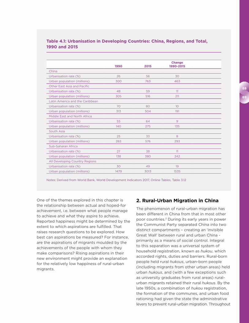
68
69
One of the themes explored in this chapter is
the relationship between actual and hoped-for
achievement, i.e. between what people manage
to achieve and what they aspire to achieve.
Reported happiness might be determined by the
extent to which aspirations are fulfilled. That
raises research questions to be explored. How
best can aspirations be measured? For instance,
are the aspirations of migrants moulded by the
achievements of the people with whom they
make comparisons? Rising aspirations in their
new environment might provide an explanation
for the relatively low happiness of rural-urban
migrants.
2. Rural-Urban Migration in China
The phenomenon of rural-urban migration has
been different in China from that in most other
poor countries.2 During its early years in power
the Communist Party separated China into two
distinct compartments – creating an ‘invisible
Great Wall’ between rural and urban China -
primarily as a means of social control. Integral
to this separation was a universal system of
household registration, known as hukou, which
accorded rights, duties and barriers. Rural-born
people held rural hukous, urban-born people
(including migrants from other urban areas) held
urban hukous, and (with a few exceptions such
as university graduates from rural areas) rural-
urban migrants retained their rural hukous. By the
late 1950s, a combination of hukou registration,
the formation of the communes, and urban food
rationing had given the state the administrative
levers to prevent rural-urban migration. Throughout
Table 4.1: Urbanisation in Developing Countries: China, Regions, and Total, 1990 and 2015
1990 2015Change
1990-2015
China
Urbanisation rate (%) 26 56 30
Urban population (millions) 300 763 463
Other East Asia and Pacific
Urbanisation rate (%) 48 59 11
Urban population (millions) 305 516 211
Latin America and the Caribbean
Urbanisation rate (%) 70 80 10
Urban population (millions) 313 504 191
Middle East and North Africa
Urbanisation rate (%) 55 64 9
Urban population (millions) 140 275 135
South Asia
Urbanisation rate (%) 25 33 8
Urban population (millions) 283 576 293
Sub-Saharan Africa
Urbanisation rate (%) 27 38 11
Urban population (millions) 138 380 242
All Developing Country Regions
Urbanisation rate (%) 30 49 19
Urban population (millions) 1479 3013 1535
Notes: Derived from World Bank, World Development Indicators 2017, Online Tables, Table 3.12
World Happiness Report 2018
the period of central planning the movement
of people, and especially movement from the
communes to the cities, was strictly controlled
and restricted.
Even after economic reform began in 1978,
migration was very limited although temporary
migration was permitted when urban demand
for labour exceeded the resident supply. The
hardships and disadvantages facing temporary
migrants holding rural hukous caused many to
prefer local non-farm jobs whenever they were
available.3 When, increasingly, migrants holding
rural hukous began to settle in the cities with
their families, they faced discrimination in access
to jobs, housing, education and health care. City
governments favoured their own residents, and
rural-urban migrants were generally treated as
second class citizens.4 For instance, they were
allowed only into the least attractive or remuner-
ative jobs that urban hukou residents shunned;
many entered self-employment, which was less
regulated. Although the urban labour markets
for urban-hukou and rural-hukou workers have
become less segmented over time, the degree of
competition between them remained very limited
in 2002.5 The tough conditions experienced by
rural-urban migrants living in urban China might
provide another explanation for their lower
happiness.
Despite these drawbacks, rural-urban migration
has burgeoned as the controls on movement
have been eased and the demand for urban
labour has increased. A study drawing on official
figures, reported that the stock of rural-urban
migrant workers was 62 million in 1993 and 165
million in 2014, in which year it represented 43%
of the urban labour force.6 An extrapolation from
the 2005 National Ten Percent Population Survey
on the basis of forecast urban hukou working
age population and of assumed urban employment
growth derived a stock of rural-hukou migrant
workers in the cities of 225 million in 2015,
having been 125 million in 2005.7 Despite the
difficulties of concept, definition and measurement
(which no doubt explain much of the difference
between the estimates for 2014 and 2015), it is
very likely the case that China is indeed experi-
encing ‘the greatest migration in human history’.
Although a large percentage of migrants come
temporarily to the cities with the intention of
returning home, an increasing percentage wish
to settle in the cities, and are establishing urban
households. As Figure 4.1 below suggests, and
as evidence of migrant wages in urban China
confirms8, the prospect of income gain was the
likely spur to the great migration.
3. Overview of Rural-Urban Migration in China
This study is based on an urban sample of rural-
urban migrant households collected as part of a
national household-based survey.9 The survey was
conducted by the National Bureau of Statistics
early in 2003 and its information generally relates
to 2002. There was no repeat interviewing of the
same households although there were some
questions that required recall of the past or projec-
tion of the future. The urban and rural samples were
sub-samples of the official annual national house-
hold survey. However, because the official urban
survey covered only households possessing urban
hukous and did not yet cover households possessing
rural hukous, the rural-urban migrant sample was
based on a sampling of households living in
migrant neighbourhoods in the selected cities.
Migrants living on their own temporarily in the
city before returning to the village were excluded.
The migrant survey contains a great deal of
information about the household and each of
its members, including income, consumption,
assets, housing, employment, labour market
history, health, education, and rural links. Less
commonly, various migrant attitudes and
perceptions were explored. The great advantage
of this survey is that the separate questionnaire
module on subjective well-being contained
specially designed questions that help to answer
the questions posed in this chapter.
The question on subjective well-being that was
asked of one of the adults in each sampled
household was: “Generally speaking, how happy
do you feel nowadays”? The six possible answers
were: very happy, happy, so-so, not happy, not at
all happy, and don’t know. They were converted
into cardinal scores as very happy = 4, happy = 3,
so-so = 2, not happy = 1, and not at all happy = 0;
the small number of don’t knows were not used
for the analysis. The happiness variable is critical
for our analysis as it is the dependent variable in
the happiness functions that are estimated to
explain happiness.
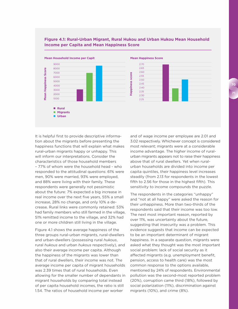
70
71
It is helpful first to provide descriptive informa-
tion about the migrants before presenting the
happiness functions that will explain what makes
rural-urban migrants happy or unhappy. This
will inform our interpretations. Consider the
characteristics of those household members
– 77% of whom were the household head - who
responded to the attitudinal questions: 61% were
men, 90% were married, 93% were employed,
and 88% were living with their family. These
respondents were generally not pessimistic
about the future: 7% expected a big increase in
real income over the next five years, 55% a small
increase, 28% no change, and only 10% a de-
crease. Rural links were commonly retained: 53%
had family members who still farmed in the village,
51% remitted income to the village, and 32% had
one or more children still living in the village.
Figure 4.1 shows the average happiness of the
three groups rural-urban migrants, rural-dwellers
and urban-dwellers (possessing rural hukous,
rural hukous and urban hukous respectively), and
also their average income per capita. Although
the happiness of the migrants was lower than
that of rural dwellers, their income was not. The
average income per capita of migrant households
was 2.39 times that of rural households. Even
allowing for the smaller number of dependants in
migrant households by comparing total instead
of per capita household incomes, the ratio is still
1.54. The ratios of household income per worker
and of wage income per employee are 2.01 and
3.02 respectively. Whichever concept is considered
most relevant; migrants were at a considerable
income advantage. The higher income of rural-
urban migrants appears not to raise their happiness
above that of rural dwellers. Yet when rural-
urban households are divided into income per
capita quintiles, their happiness level increases
steadily (from 2.13 for respondents in the lowest
fifth to 2.56 for those in the highest fifth). This
sensitivity to income compounds the puzzle.
The respondents in the categories “unhappy”
and “not at all happy” were asked the reason for
their unhappiness. More than two-thirds of the
respondents said that their income was too low.
The next most important reason, reported by
over 11%, was uncertainty about the future,
suggesting that insecurity was a problem. This
evidence suggests that income can be expected
to be an important determinant of migrant
happiness. In a separate question, migrants were
asked what they thought was the most important
social problem: lack of social security as it
affected migrants (e.g. unemployment benefit,
pension, access to health care) was the most
common response to the options available,
mentioned by 24% of respondents. Environmental
pollution was the second-most reported problem
(20%), corruption came third (18%), followed by
social polarization (11%), discrimination against
migrants (10%), and crime (8%).
Figure 4.1: Rural-Urban Migrant, Rural Hukou and Urban Hukou Mean Household Income per Capita and Mean Happiness Score
Mean Household Income per Capit Mean Happiness Score
2.70
2.65
2.60
2.55
2.50
2.45
2.40
2.35
2.30
2.25
9000
8000
7000
6000
5000
4000
3000
2000
1000
Me
an
Hap
pin
ess
Sco
re
Hap
pin
ess
sco
re
Rural Migrants Urban

World Happiness Report 2018
Migrants were also asked: “Compared with your
experience of living in the rural areas, are you
happier living in the city”? No fewer than 56% felt
that urban living gave them greater happiness,
41% reported themselves equally happy in rural
and urban life, while only 3% reported greater
rural happiness. When asked what they would do
if forced to leave the city, more migrants would
go to another city (54%) than would go back to
their village (39%). These results add to the
puzzle. If most migrants view urban living as
yielding them greater happiness, and most wish
to remain in an urban area, why are their mean
happiness scores lower than those of rural
residents?
4. Possible Explanations
There are several possible explanations for these
results. The first possibility is that migrants, when
they decided to migrate from the village, had
excessively high expectations of the conditions
that they would experience in the city. We shall
look for evidence that this might be the case by
considering the characteristics of their urban life
that reduce their welfare.
Second, the puzzle might be solved by recourse
to the possibility of adaptation, following Easterlin’s
evidence.10 He argues that happiness depends
both on income and aspirations, the former
having a positive and the latter a negative effect.
Moreover, as income rises over time, aspirations
adapt to income, so giving rise to what has been
called a ‘hedonic treadmill’.11 When respondents
are asked to assess how happy they had been in
the past, when their income was lower, they tend
to judge that situation by their current aspirations
for income and therefore to report that they are
more happy now. Similarly, when they are asked
to assess their happiness in the future, when they
expect to have higher income, they do not realise
that their aspirations will rise along with their
income and therefore report that they will be
happier. This is possibly because, as findings
from social psychology suggest, ‘We don’t always
predict our own future preferences, nor even
accurately assess our experienced well-being
from past choices’.12
If current judgements about subjective well-
being, whether in the past, the present, or the
future, are based only on aspirations in the
present, this might explain why migrants on
average are less happy than rural people:
aspirations could have risen after having made
the decision to migrate. While aspirations might
not be directly measurable, the implications of
adaptation can be tested. Similarly, we might also
find an explanation for why it is that migrants
generally report that their happiness is higher, or
at least no lower, in urban than in rural areas.
A second possibility is that people form their
aspirations relative to some ‘reference group’, i.e.
the people with whom they compare themselves.
The reference group can change when they
move to the city and find themselves with richer
neighbours. The notion that aspirations depend
on income relative to that of the relevant reference
group comes from the sociological literature,13
and has been developed for China in related
papers on subjective well-being.14 The literature
on relative income was well summarised and
evaluated in 2008,15 since when many more
studies of the effects of relative income have been
made, albeit mainly for developed economies.
Other studies for developing countries which
show the importance of reference groups include
shifts in reference norms in Peru and Russia,16
comparison with close neighbours in South
Africa,17 and rural-urban migrants retaining a
village reference group in Nepal.18 If the group
with which the migrants compare themselves
changes as a result of rural-urban migration
and urban settlement, this might explain why
their aspirations change. We can test whether
migrants show ‘relative deprivation’ in relation
to urban society.
Our third possibility is that the presence of
members left behind in the village can place a
burden on the urban members of the two-location
family. Insofar as migrants remit part of their
income, their own happiness score might fall and
that of their rural family rise. Equivalently, our
measure of the income per capita of the urban
migrant household might overstate its disposable
income per capita.
Fourth, our results might be explained by the
untypical nature of the migrants. The lower
happiness of migrants may be the result of their,
or of their households, having characteristics
different from those of the rural population as a
whole. If this were the case, they could indeed
have been less happy on average had they
72
73
remained in the village. Such happiness-reducing
characteristics might be captured by the survey
data – and thus be capable of being accounted
for in the statistical estimations - or they might
be unobservable to the researcher. For instance,
it is possible that those rural-dwellers who by
nature are melancholy or have high and unfulfilled
aspirations hold their rural life to be responsible
and expect that migration will provide a cure.
They might therefore be more prone to leave the
village for the city. If the self-selected migrants
are intrinsically less happy, this might explain
why the sample of rural-urban migrants has a
lower average happiness score than does the
sample representative of the rural population of
which they were previously a part. Self-selection
of this sort might also involve false expectations,
in this case based on self-misdiagnosis. Its
implications can be tested.
5. The Determinants of Happiness
Happiness functions were estimated to discover
the factors associated with the happiness of
rural-urban migrants19 so as to test the possible
explanations 1, 2 and 3, just outlined. We proceed
in stages: first, we estimate ordinary least
squares (OLS) estimates of the happiness score
with a full set of explanatory variables. Second,
we investigate whether these explanatory variables
have different effects on happiness depending
on the length of time that the household had
been living in urban areas by dividing the migrant
sample into ‘short-stayers’ and ‘long-stayers’, i.e.
those who had settled in the city for less and more
than the median time (7.5 years) respectively.
Third, we confine the sample to employed
migrants, as this enables us to see whether
working conditions, denoted by work-related
variables, have an impact on happiness. However,
because the full results are available elsewhere
(Knight and Gunatilaka, 2009, 2012, on which
this chapter draws heavily) we report only the
variables that are critical for our story.
Table 4.2 reports, for the full sample but with only
the most relevant variables shown, the average
values of the explanatory variables (column 1)
and then coefficients in the happiness function
estimated with the full set of available explanatory
variables (column 2). With the happiness score
as the dependent variable (the variable to be
explained) and various independent variables
(chosen as the explanatory variables), the
estimated ‘coefficients’ on the explanatory
variables indicate the effect on happiness made
by a unit change in each explanatory variable,
holding all other explanatory variables constant.
The asterisks show levels of statistical significance:
the more asterisks against a coefficient, the more
statistically significant is the effect on happiness.
In column 2, the coefficient on log of income per
capita is significantly positive, and its value
(0.20) indicates that a doubling of income raises
the happiness score by about 0.14 points. Income
is relevant, as predicted, but its effect does not
appear powerful by comparison with either the
presumptions of economists or the estimated
effects of some other variables. For example,
reporting to be in good health (rather than not in
good health) raises the happiness score by 0.12
points according to column 2.
Migrants can be expected to adjust over time to
urban life in various ways. On the one hand, as
they overcome initial difficulties and become
more settled, we expect their happiness to rise.
On the other hand, their reference groups might
change, from the poorer, village society to the
richer, urban society, and this fall in perceived
comparative status might reduce happiness. The
length of time spent in the urban area is introduced
as an explanatory variable, and also its square so
as to allow the possibility that the relationship is
curved rather than being a straight line. The
variable and its square are both significant, the
former positively and the latter negatively
although only at the 10% critical level. The
coefficients imply that the happiness score rises
to a peak after 12 years and then declines.
However, it is possible that there is selective
settlement: happier migrants are more likely to
choose to stay long in the city. This would tend to
bias upwards the estimated returns to duration of
urban residence. In summary, it would appear
that migrants’ happiness tends to rise over several
years of urban living, but the evidence is weak.
In order to pursue the notion that reference
groups can be important, the effect of relative
income was investigated. Drawing on the urban
and rural samples of the 2002 national house-
hold survey, the average urban income per capita
in the destination city and (lacking information
on the origin county) the average rural income
per capita in the origin province of the migrant,
are introduced. The expectation is that both have
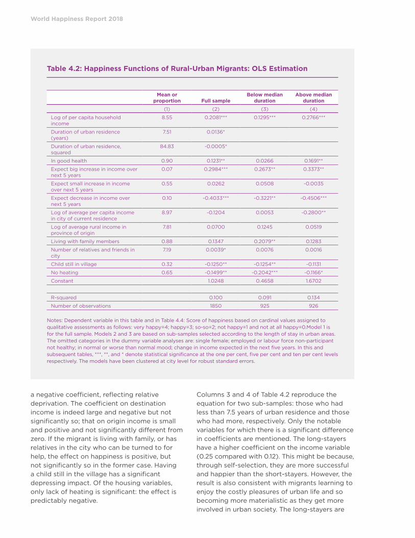
World Happiness Report 2018
a negative coefficient, reflecting relative
deprivation. The coefficient on destination
income is indeed large and negative but not
significantly so; that on origin income is small
and positive and not significantly different from
zero. If the migrant is living with family, or has
relatives in the city who can be turned to for
help, the effect on happiness is positive, but
not significantly so in the former case. Having
a child still in the village has a significant
depressing impact. Of the housing variables,
only lack of heating is significant: the effect is
predictably negative.
Columns 3 and 4 of Table 4.2 reproduce the
equation for two sub-samples: those who had
less than 7.5 years of urban residence and those
who had more, respectively. Only the notable
variables for which there is a significant difference
in coefficients are mentioned. The long-stayers
have a higher coefficient on the income variable
(0.25 compared with 0.12). This might be because,
through self-selection, they are more successful
and happier than the short-stayers. However, the
result is also consistent with migrants learning to
enjoy the costly pleasures of urban life and so
becoming more materialistic as they get more
involved in urban society. The long-stayers are
Table 4.2: Happiness Functions of Rural-Urban Migrants: OLS Estimation
Mean or
proportion Full sampleBelow median
durationAbove median
duration
(1) (2) (3) (4)
Log of per capita household income
8.55 0.2081*** 0.1295*** 0.2766***
Duration of urban residence (years)
7.51 0.0136*
Duration of urban residence, squared
84.83 -0.0005*
In good health 0.90 0.1231** 0.0266 0.1691**
Expect big increase in income over next 5 years
0.07 0.2984*** 0.2673** 0.3373**
Expect small increase in income over next 5 years
0.55 0.0262 0.0508 -0.0035
Expect decrease in income over next 5 years
0.10 -0.4033*** -0.3221** -0.4506***
Log of average per capita income in city of current residence
8.97 -0.1204 0.0053 -0.2800**
Log of average rural income in province of origin
7.81 0.0700 0.1245 0.0519
Living with family members 0.88 0.1347 0.2079** 0.1283
Number of relatives and friends in city
7.19 0.0039* 0.0076 0.0016
Child still in village 0.32 -0.1250** -0.1254** -0.1131
No heating 0.65 -0.1499** -0.2042*** -0.1166*
Constant 1.0248 0.4658 1.6702
R-squared 0.100 0.091 0.134
Number of observations 1850 925 926
Notes: Dependent variable in this table and in Table 4.4: Score of happiness based on cardinal values assigned to qualitative assessments as follows: very happy=4; happy=3; so-so=2; not happy=1 and not at all happy=0.Model 1 is for the full sample. Models 2 and 3 are based on sub-samples selected according to the length of stay in urban areas. The omitted categories in the dummy variable analyses are: single female; employed or labour force non-participant not healthy; in normal or worse than normal mood; change in income expected in the next five years. In this and subsequent tables, ***, **, and * denote statistical significance at the one per cent, five per cent and ten per cent levels respectively. The models have been clustered at city level for robust standard errors.

74
75
more sensitive to average urban income per
capita in the destination city (a significant -0.28
compared with a non-significant -0.01). This
suggests that over time urban residents increas-
ingly become the reference group for migrants.
Moreover, the fact that this makes them relatively
less happy might explain why additional income
becomes more important for their happiness.
The sensitivity of happiness to relative income in
the destination city, especially for long-stayers,
seems to agree with our second possible
explanation, i.e. that migrants’ aspirations rise as
they adjust to their new urban environment. The
extreme sensitivity of migrant happiness scores
to income rank in the city (shown in Table 4.5
below) provides further supporting evidence.
These results were found to be unchanged using
alternative versions of the happiness variable20.
An attempt was also made to examine the
sensitivity of our results to the influence of the
unobserved determinants of happiness.21 For
instance, unobserved characteristics such as
personal energy might raise both income and
happiness, or happiness itself might improve
motivation and so raise income. The income
variable was therefore adjusted to correct for
such unobserved influences, but the results of
this exercise did not alter our story.22
We investigated the effect of working
conditions on the subjective well-being of
employed respondents. In other words, does
the unpleasantness and insecurity of urban work
contribute to the unhappiness of migrants?
Table 4.3 is based on estimates of the full sample
equation of Table 4.2 but for employed respondents
only, the reason being that it is then possible to
add various employment-related explanatory
variables.23 The first column provides mean
values and the second shows only the results for
the additional variables as the coefficients of the
variables in common barely change.
Where satisfaction with the current job is rated 4
for ‘very satisfied’ down to 0 for ‘not at all
satisfied’, this variable has the expected positive
and significant coefficient. Respondents were
asked whether rural workers enjoyed the same
treatment as urban workers in seven different
aspects of the employment relationship. The
negative answers were added to form an index
of discrimination (ranging from 0 to 7). The
coefficient is negative and significant, indicating
that perceptions of discrimination contribute
to unhappiness. Compared with being self-
employed, having permanent work or long term
contract work raises happiness but this result is
not statistically significant, i.e. it could arise by
Table 4.3: Happiness Functions of Employed Rural-Urban Migrants: OLS Estimation
Mean or proportion Coefficient
Satisfaction with job 1.98 0.0735*
Index of discrimination 5.35 -0.0322***
Permanent or long-term contract work 0.05 0.1338
Temporary work 0.24 0.0079
Can find another job in two weeks 0.11 -0.0997
Can find another job in a month 0.23 -0.1213**
Can find another job in 2 months 0.10 -0.1478*
Can find another job in 6 months 0.13 -0.1917**
Need more than 6 months to find another job 0.17 -0.2140***
R-squared 0.129
N 1715
Notes: With the addition of employment-related variables, the specification of column 2 is identical to that of column 2 of Table 4.3, but the variables presented in Table 4.3 are not reported. The omitted categories in the dummy variable analyses reported are: self-employed; can find a job immediately. The equation has been clustered at city level for robust standard errors.
World Happiness Report 2018
chance. Another aspect of the insecurity of
urban employment can also be incorporated.
Respondents were asked how long it would take
them to find another job with equivalent pay if
they lost their current job. Compared with ‘within
one week’ - the reference category with which
other categories are compared - the coefficients
are generally significantly negative and increase
steadily in size. The evidence is consistent with
our first possible explanation: migrant employ-
ment can be unpleasant and insecure, and this
depresses migrant happiness.
The third possible explanation emerges from
theories of rural-urban migration expressed in
terms of decision-making by the rural family, of
which the migrant remains a part. The inference
is that the average happiness score of migrants
is low because they support their rural family
members by remitting part of their income to
them. In that case, our dependent variable
cannot reflect the full gain in happiness of the
two-location family. In principle the argument is
weak. First, it is less plausible for settled than for
temporary migrants. Second, ‘utility-maximising
economic agents’ (a concept commonly used by
economists!) are assumed to allocate their
income optimally, i.e. at the margin gifts yield
as much utility for the giver as consumption.
Altruism and satisfaction that they are fulfilling
their family obligations might raise migrants’
happiness. So happiness need not fall if income
is remitted. It is nevertheless true that migrant
household disposable income per capita is often
reduced by the presence of family members
elsewhere.
It is relevant that 51% of migrant households made
remittances, and that remittances represented 9%
of household income for the sample as a whole
and 17% for the remitting households. Do
remittances reduce the happiness of respondents
in migrant urban households, and so contribute
to the low average happiness score? If that were
the case, the variable log of household remittance
per capita would be significantly negative in the
estimated happiness function.24 However, whether
this term is added to the full estimated equation
or the sub-sample of remitters, the coefficient on
the remittance variable remains no different from
zero. To illustrate, when the variable log remittances
per capita is added to column 2 of Table 4.2
(not shown), the coefficient is a non-significant
0.0064. Thus, we found no evidence in support
of the third possible explanation, i.e. that migrants’
happiness is reduced because they remit part of
their income,
6. Why Are Migrants Less Happy Than either Rural Dwellers or Urban Dwellers?
Migrants might be less happy on average than
either rural or urban people because they differ
in their average characteristics, i.e. average
endowments of happiness-affecting attributes
such as health status. Here a different testing
methodology is required. The migrants are
compared with both rural and urban residents,
employing a standard decomposition technique.
The objective is to pinpoint the reasons for the
difference in happiness. The decomposition
shows the contribution to the difference in
happiness that is made by each determinant
of happiness.
We began by conducting a decomposition
analysis of the difference in household mean
income per capita, in order to throw some light
on the representativeness and the motivation of
the migrants. The decomposition methodology is
explained in the technical box below, where it is
illustrated in terms of differences in average
happiness. Those migrating from rural China are
indeed a selective and unrepresentative group.
Migrant households, had they remained in the
rural areas, would on average earn 10% less
income than do rural resident households. There
is also a considerable income advantage to their
migration: the average income that migrant
households actually earn is 2.64 times what they
would earn in the rural areas. By contrast, if they
were to migrate, average rural households would
earn 2.19 times more than they actually earn. It
appears that rural households possess productive
characteristics that are relatively valuable in the
countryside whereas migrant households possess
productive characteristics that are relatively
valuable in the city.
The average happiness score of rural people
was 2.68 and that of migrants 2.37, implying a
migrant shortfall of 0.31. Table 4.4 decomposes
this gap into the parts which can be explained
by differences between the two groups in the
average values of their characteristics and
by differences in the coefficients in the two

76
77
happiness functions. The figures show the
percentage contributions of the difference in
average values of characteristics and of the
difference in coefficients respectively.
We see from the first column of Table 4.4 that
the share of the difference in average happiness
scores that is attributable to differences in
average characteristics sums to -35%, and from
the second column that the share attributable
to differences in coefficients sums to 135%. The
effect of characteristics is therefore actually to
increase the difference in mean happiness scores.
This is mainly due to the variable log of income
per capita: the effects of income are the same
in the two samples but migrants have higher
incomes. The reason why migrants have lower
average happiness must therefore be found in
the different explanations for the happiness of
the rural and urban residents, based on their
different coefficients. The constant term, health,
and income expectations are the main
contributors, and age is the big exception.
The importance of the constant term implies
that there are unobserved characteristics that
we have not been able to include in the model
which reduce migrant relative to rural happiness.
For example, we are unable to standardise for
the various social disadvantages that migrants
encounter in the cities because the same
variables are not available in the rural data set.
Perhaps because rural people are on average
less healthy than migrants - poor health being
a deterrent to migration - they place a higher
value on good health.
In both samples happiness is highly sensitive to
expectations about future income in five years’
time. It appears from Figure 4.2 that expectations
of future income can influence current happiness.
With the expectation of no change in income as
the reference category in the dummy variable
Technical Box
The Blinder-Oaxaca decomposition technique is employed to explain the difference in
mean happiness between migrant and rural households. This is based on identical happiness
regression equations for the two groups being compared. The choice of explanatory
variables used is governed by the availability of the same variable in the two data sets, and
by whether it is a successful predictor of happiness in the estimated happiness functions.
The decomposition is based on two equations:
Hr – H
m = X
m (a
r – a
m) + a
r (X
r – X
m), (1)
and
Hr – H
m = X
r (a
r – a
m) + a
m (X
r – X
m). (2)
In the equations, Hr, H
m are the mean happiness scores in the rural and migrant samples
respectively, Xr, X
m are vectors of rural and migrant mean characteristics, and a
r, a
m are
vectors of rural and migrant coefficients. Equation (1) enables us to pose the counterfactual
question ‘what would be the effect on the mean happiness of migrants if they had the
same happiness function as rural people?’, and equation (2) the question ‘what would be
the effect on the mean happiness of rural people if they had the same happiness function
as migrants?’ To illustrate the decomposition according to equation (2), the entry -55.39 in
row 1, column 1 of Table 4.4 is obtained by multiplying the difference in mean log of income
per capita by the migrant coefficient of log of income per capita, and the entry 1.01 in row
1, column 2 by multiplying the mean rural log of income per capita by the difference in
coefficients, and then expressing these products as percentages of the gross mean difference
in happiness. Only the decomposition based on equation (2) is reported in the table.
However, the results for the alternative decomposition are very similar.

World Happiness Report 2018
analysis, the coefficients in the migrant sample
vary from 0.31, if a large increase is expected, to
0.05, if a small increase is expected, and to -0.39,
if a decrease is expected; the corresponding
estimates for the rural sample are 0.41, 0.19 and
-0.19 respectively. The fact that in the migrant
sample the coefficients are uniformly lower, in
relation to the expectation of static income,
suggests that migrants have higher aspirations
relative to their current income. This can be
expected if aspirations depend on the income of
the relevant comparator group. Whereas the
Table 4.4: Decomposition of the Difference in Mean Happiness Score between Rural-Urban Migrants and Rural Residents: Percentage Contribution to the Difference
Using the migrants’ happiness function
Due to characteristics Due to coefficients
Log of income per capita -55.39 1.01
Health -5.81 94.41
Income expectations 11.34 36.36
Age 6.69 -131.54
Other variables 7.95 5.48
Sum (percentage) -35.23 135.23
Sum (score) -0.1078 0.4137
Notes: The mean happiness scores are 2.6764 in the case of rural residents and 2.3703 in the case of migrants, creating a migrant shortfall of 0.3061 (set equal to +100%) to be explained by the decomposition. This represents 100 per cent. The composite variables are age and age squared for age, married, single, divorced and widowed for marital status, and big increase, small increase and decrease for income expectations. ‘Other variables’ included in the equation but not reported are education, age, male, marital status, ethnicity, CP membership, unemployment, working hours, and net financial assets.
Figure 4.2: Rural-Urban Migrant and Rural Dweller Coefficients Of Variables Denoting Expectations of Income in the Next Five Years, Derived from the Happiness Equations Estimated for Table 4.4
0.50
0.40
0.30
0.20
0.10
0.00
-0.10
-0.20
-0.30
-0.40
-0.50
Co
effi
cie
nts
R-U migrants Rural dwellers
Expect big increase in income
Expect small increase in income
Expect decrease in income

78
79
rural respondents are fairly representative of
rural society, and so their mean income is close
to the mean income of their likely comparator
group, the migrant sub-sample is unrepresentative
of urban society: migrants tend to occupy the
lower ranges of the urban income distribution. If
migrants make comparisons with urban-born
residents, their aspirations will be high in relation
to their current income.
Is the low mean happiness of migrants a general
characteristic of city life? The inquiry can be
pursued further by comparing migrants with
‘urban residents’, i.e. persons who are urban-born
and or in other ways have acquired urban hukou
status, with the rights and privileges that
accompany it. The average happiness score of
urban residents is 2.48 and that of migrants
2.37, implying a migrant shortfall of 0.11. Table 4.5
provides a decomposition exercise similar to that
of Table 4.4 but with a different set of explanatory
variables - those that are common to the two
datasets.
In this case the differences in coefficients
add slightly to the migrant shortfall in average
happiness score (in total, coefficients’ share of
the explanation for the difference in average
happiness is -21%). The coefficient on the income
variable is higher for urban residents (0.173) than
for migrants (0.111), so raising urban relative to
migrant happiness. The positive effect of income
expectations reflects the lower coefficients in the
migrant sample: with static expectations as the
reference category, for migrants an expected big
increase in income has a coefficient of 0.21, a
small increase 0.00, and a decrease -0.37, whereas
for urban residents the corresponding estimates
are 0.34, 0.10, and -0.29 respectively. Again,
migrants appear to have higher aspirations
relative to their current income.
The contribution of the various income coefficients
to the explanation of the difference in mean
happiness is offset by the negative effects of
such variables as age, gender and the constant
term. Note that position in the city income
distribution has a powerful effect on happiness.
With the highest quarter of households being the
omitted category, the happiness coefficient falls
monotonically, to lower than -0.80 in the lowest
Table 4.5: Decomposition of the Difference in Mean Happiness Score between Rural-Urban Migrants and Urban-Hukou Residents: Percentage Contribution to the Difference
Using the migrants’ happiness function
Due to characteristics Due to coefficients
Log of income per capita 28.15 472.62
Income expectations -39.92 59.32
Living standard in second highest quarter in city -33.68 26.28
Living standard in third highest quarter in city -11.71 77.84
Living standard in lowest quarter in city 175.93 -8.37
Age 32.85 -594.05
Male -4.08 -46.78
Health -28.01 51.89
Other variables 1.14 36.97
Constant term 0.00 -96.38
Sum (percentage) 120.67 -20.67
Sum (score) 0.1342 -0.0230
Notes: The mean happiness scores are 2.4845 in the case of urban residents and 2.3703 in the case of migrants, creating a migrant shortfall of 0.1143 (set equal to +100%) to be explained by the decomposition. This represents 100 per cent. The composite variables are age and age squared for age, married, single, divorced and widowed for marital status, and big increase, small increase and decrease for income expectations. ‘Other variables’ are education, marital status, ethnicity, CP membership, unemployment, working hours and net financial assets.

World Happiness Report 2018
quarter. As this is true of both samples, it does
not affect relative happiness.
The migrant shortfall in happiness therefore has
to be explained in terms of differences in average
characteristics (the total share of characteristics in
accounting for the difference in average happiness
is 121%). Two variables stand out: the higher
mean income of urban residents improves their
relative happiness, and their superior position in
the city income distribution has the same effect.
A far higher proportion of migrants than of urban
residents fall in the lowest quarter of city house-
holds in terms of living standard (35% compared
with 11%). This fact alone can explain more than
the entire migrant deficit. If the income of the
relevant comparator group influences aspirations,
the inferior position of migrants in the city
income distribution can also explain why they
appear to have higher aspirations in relation to
their current income.
7. Are Migrants Self-Selected?
It is evident that differences in unobserved
characteristics are important for the differences
in happiness. For example, the constant term in
the decomposition presented in Table 4.4 explains
more than the entire difference in the average
happiness scores of migrants and rural-dwellers.
Migrants might be less happy on average simply
because inherently unhappy people tend to be
the ones who migrate. Support for this idea comes
from answers to the question as to whether urban
living had yielded greater happiness than rural
living. Despite the average happiness score being
lower for migrants than for rural people, 56% of
migrants thought that urban living made for
greater happiness and only 3% disagreed. This is
the picture that could emerge if migrants are
intrinsically unhappy people whose happiness
remains low despite improving after migration.
Migrants might be unhappy people because by
nature they are melancholy or they have high but
unfulfilled aspirations. However, the latter reason
fits ill with the stereotype of migrants as relatively
self-confident, optimistic, risk-loving individuals.
Consider the implications of assuming both that
migrants are naturally unhappy people and that
migration does indeed generally raise happiness.
Insofar as those migrants with a relatively unhappy
disposition become absolutely happier albeit still
relatively unhappy after migration, we might
expect as high a proportion of unhappy as of
happy migrants to report that their life is more
satisfactory in urban than in rural areas. In fact
the proportion falls, from 67% in the highest
happiness category to 34% in the lowest
Figure 4.3: Rural-Urban Migrant and Urban Dweller (with Urban Hukou) Coefficients of Variables Denoting Expectations of Income in the Next Five Years, Derived from Happiness Functions Estimated for Table 4.5
0.50
0.40
0.30
0.20
0.10
0.00
-0.10
-0.20
-0.30
-0.40
-0.50
Co
effi
cie
nts
R-U migrants Urbanl dwellers
Expect big increase in income
Expect small increase in income
Expect decrease in income

80
81
happiness category, suggesting that this sort
of self-selection can at best be only a partial
explanation for the lower average happiness
of migrants.
The Technical Box below explains how it was
possible to isolate that part of the happiness of
each migrant that cannot be explained by our
variables. We could then test whether this
residual helps to explain the respondent’s report
that they are happier in the city than in the
village. Table 4.6, predicting an affirmative answer,
identifies the characteristics which have raised
happiness. When the residual is introduced
into the equation (column 2) the prediction is
that it will not be different from zero if inherent
and unchanging personality is the cause of
unhappiness. However, the positive effect
suggests that migration changed the unobserved
characteristics of migrants. In that case inherent
disposition cannot solve out puzzle.
Instead, migrants might select themselves on
the basis of unobserved characteristics that are
different or have different effects in the two
locations. Several examples come to mind
(beyond the case discussed under our second
possible explanation, i.e. migrants’ aspirations
rise). If people who are dissatisfied with life in
general but with village life in particular have a
high propensity to migrate, migrants might have
low average happiness in both locations but
particularly in the village. For instance, own
or family misfortune or bad family or village
relationships could reduce a person’s happiness
but more so if they remained in the village. If
migrants have high pre-existing aspirations
which cannot be fulfilled in the village but have
the potential to be better met in the city, this
might have the same effect. In each of these
cases the migrants would be likely to report that
their urban life is better than their rural life had
Table 4.6: Determinants of Urban Living Happier than Rural Living: Employed Sample, Probit Estimation
Marginal Effects of Probit Estimation
(1) (2)
Log of per capita household income 0.0506* 0.0466*
Duration of urban residence (years) 0.0174*** 0.0190***
Duration of urban residence, squared -0.0003 -0.0004
Expect big increase in income over next 5 years 0.1657** 0.1766***
Expect small increase in income over next 5 years 0.0869** 0.0941***
Expect decrease in income over next 5 years -0.0557 -0.0559
Difference between actual and predicted happiness score 0.1736***
Living with family members 0.1286** 0.1070*
Living in own house 0.1304** 0.1286**
Satisfaction with job 0.0719*** 0.0768***
Number of observations 1715 1715
Notes: The dependent variable is the probability of being happier in urban areas. For the dummy variables denoted by (d), the marginal effects are denoted by dy/dx for discrete change of dummy variable from 0 to 1.
The variable, difference between actual and predicted happiness score, has been derived by obtaining predicted happiness score from estimating Model (1) in Table 4.3.The omitted categories in the dummy variable analyses are: single female; employed or labour force non-participant; not healthy; in normal or worse than normal mood; change in income expected in the next five years. Explanatory variables estimated in the equations but not reported in the table are: male, married, male and married, education, working hours, net financial assets, ln average household per capita income in city of current residence, ln household per capita rural income in province of origin,, permanent or long-term contract work, index of discrimination, can find another job in two weeks, .one month, two months, six months, needs more than six months to get another job. The equations have been clustered at city level for robust standard errors.

World Happiness Report 2018
been, despite their low average urban happiness.
A test of this type of explanation would require
a survey which could reveal the happiness
score, and the reasons given for unhappiness,
before migrating
8. Other China Studies
One other study deals specifically with migrants.25
It analysed the China Household Income Project
(CHIP) survey [also known as the Rural-Urban
Migration in China (RUMIC) survey] relating
mainly to 2007. The research interest is in the
effects of various measures of relative income on
happiness. The data differed from that used in
the analysis above in that it contained all rural
hukou people present in the urban areas, i.e.
both temporary and settled migrants, and the
dependent variable was an aggregation of
twelve measures of mental health.
It was found that subjective well-being is
negatively affected by the incomes of other
migrants and of workers in the home region.
However, a positive coefficient was obtained
on average income in the local urban area.
This was interpreted as a ‘signal’ effect, i.e. the
higher incomes of urban people served as a
signal of future income prospects. A similar
positive coefficient had been obtained and
similarly explained for Russia.26 It contrasts
sharply with our finding of a negative coefficient.
The contrast was explained as arising because
our sample contained only settled migrants,
who were more likely to have transferred their
reference group from the village to the city. In
support of this explanation, it was noted that
the positive coefficient declined with years
since migration. Containing very different
definitions both of a migrant and of subjective
well-being, the two analyses are not necessarily
contradictory.
Technical Box
The argument can be tested rigorously as
follows. Estimating the predicted happiness
score for each respondent (from column 2
of Table 4.2), the residual (actual minus
predicted) score is the part of happiness
that cannot be explained by our equation.
The residual is made up of measurement
error and two sorts of unobserved
characteristics of the respondent: those
which were present before migration and
those which came after migration. A
disposition to be happy or unhappy is of
the former sort. Assume that migration
had a similar effect on the happiness of
all respondents whose unobserved
characteristics did not change pre- and
post-migration. In that case, we can test
whether the residual helps to explain
whether the respondent reported that
their happiness was higher in the city than
in the village.
Table 4.6 shows the results of a Probit
regression predicting an affirmative answer.
Its two columns, presenting the marginal
effects of each explanatory variable, both
refer to the employed sample. The object is
to identify the characteristics which have
raised happiness. Comparing Tables 4.2 and
4.3 (using OLS) with Table 4.6 (using Probit),
we see that some of the same variables that
determine happiness also correspondingly
determine an increase in happiness. When
the residual is introduced into the equation
corresponding to column 2 of Table 4.6, the
expectation is that it will not be significantly
different from zero if inherent and unchanging
personality is the cause of unhappiness.
However, the coefficient is positive and
significantly so at the 1% level (column 2),
and the marginal implies that a residual of
+1.0 raises the probability of an affirmative
answer by 17 percentage points. This
positive effect suggests that migration
changed the unobserved characteristics of
migrants, in which case inherent disposition
cannot solve the puzzle.
82
83
Another study examined the changes in the
average happiness of urban, rural, and rural-
urban migrant households between the CHIP
2002 and CHIP 2013 national household surveys.27
The ratio of migrants’ to rural households’
income per capita was higher in 2013 than it had
been in 2002: again, the economist’s expectation
is that rural people would have an incentive to
migrate to raise their utility. However, the average
happiness of rural-dwellers remained higher than
that of migrants, although the gap had narrowed.
The rise in migrant happiness was probably due
to the rapid growth of their income, associated
with the growing scarcity of migrant labour, and
gradual (but minor) improvements in their urban
treatment and conditions in recent years. We
surmise that the fall in average rural happiness,
despite a rise in average rural income, was
because the loss of household members to the
cities often left unbalanced families and villages
behind, or because rural households’ aspirations
rose rapidly as their information about urban
life improved.
9. Studies in Other Developing Countries
To what extent can the China story be
generalised? In one respect – the harsh
institutional and policy treatment of rural hukou
migrants in the cities – China is likely to be
exceptional. However, in many countries rural-
urban migrants are at a disadvantage: their
social networks are often weak, their education
is liable to be of poor quality for urban life and
work, and their village customs and weak
assimilation might cause social discrimination.
However, the available evidence cannot provide
a clear answer to this question. It appears that
research on the relationship between rural-urban
migration and happiness in developing countries
remains very limited.
Whereas our China case study found that
migration may well have had the consequence
of reducing subjective well-being, a study of
Thailand found that a somewhat higher propor-
tion of the permanent migrants in that sample
experienced an increase in life satisfaction after
migration than experienced a decrease.28
The interpretation of our main finding in terms
of changing reference groups is echoed in a
pioneering study for developing countries of
aspirations relative to achievement which
examined ‘frustrated achievers’ in Peru. More
than half of those who had objectively achieved
the largest income growth subjectively reported
that their economic condition had deteriorated
over the previous decade. Part of the explanation
was to be found in their perception of increased
relative deprivation.29
In South Africa a very extensive system of
temporary circular migration prevailed in the
past. However, since the advent of democracy
the country has increasingly experienced the
permanent urban settlement of rural-dwellers.
The same question has been posed for South
Africa as was posed above for China.30 That
study reached similar results and suggested
some of the same interpretations but used a
different methodology. A longitudinal panel
survey identified the happiness of rural people
and their happiness four years later after
rural-urban migration (excluding temporary
migration). The real income of the migrants rose
substantially, largely because of their migration.
Yet sophisticated estimation yielded a fall in
subjective well-being (measured on a scale of 0
to 10) of 8.3%. A favoured interpretation was that
this reduction was the result of false expectations
and changing reference groups after the migrants
settled in the urban areas.
10. Summary and Conclusion
This chapter illustrates how it should be possible
to go beyond a description of happiness and
its correlates. Using microeconomic (individual
and household) data based on a well-designed
survey and questionnaire, microeconomic
analysis can be used to explore and to answer
interesting and important questions about what
makes people happy or unhappy. The settled
rural-urban migrants that we study are the
vanguard of a great wave of settlement as the
urban economy becomes increasingly dependent
on migrants from rural China.
We have posed the question: why do rural-urban
migrant households which have settled in urban
China report lower happiness than rural house-
holds? Migrants had lower average happiness
despite their higher average income: the income
difference merely adds to the puzzle. It is a
World Happiness Report 2018
question that cannot easily be answered in terms
of economists’ conventional models of rural-
urban migration based on ‘utility maximisation’.
Four possibilities were examined. We found
no evidence for the idea that happiness was
reduced by the need for the migrants to provide
support for family members in the village.
Each of the other three possibilities involves
false expectations, of three different types:
prospective migrants may have false expectations
about their urban conditions, or about their
urban aspirations, or about themselves. What
they have in common is that rural-urban migrants
are likely to lack the necessary information to
enable them to judge the quality of their new
lives in a different world. For each of the three
types of belief there are reasons why they are
too optimistic about life in the city.
Consider first the idea that migrants are too
optimistic about the conditions of city life. The
fact that happiness appears to rise over several
years suggests that migrants are able to over-
come the early hardships of arriving, finding
work, and settling in the city. However, some
hardships remain, relating to accommodation,
family, and work. Provided that accurate
information had been available to prospective
migrants, they should have taken account of
adverse conditions reducing their happiness
when deciding to migrate: expectations would
not have been false. Why might migrants
overestimate the conditions of their urban life
and work? It is possible that, whereas expected
income is quantifiable and understandable, other
aspects of urban life have to be experienced
to be understood. Moreover, expectations of
conditions might be based on images of the
lives of urban residents rather than those of
rural-urban migrants, or the reports provided
by migrant networks might be too rosy. The
migrants, when they made their decisions to
move, may have been realistic about their urban
income prospects, whereas their expectations
of living and working conditions could have been
biased upwards. However, there is a caveat:
the better the information flows to the villages,
the weaker is the case for this possibility.
The second possibility is that migrants had
falsely believed, at the time of migration, that
their aspirations would not alter in the city.
Consider the reasons why migrants’ aspirations
may have risen and now exceed their actual
achievements. When we conducted a decompo-
sition analysis to discover why migrants have a
lower mean happiness score than both rural
dwellers and urban dwellers possessing urban
hukous, in each case a major contribution came
from the higher aspirations of migrants in relation
to current income. This is consistent with the fact
that over two-thirds of migrants who were
unhappy or not at all happy gave low income as
the predominant reason for their unhappiness.
The relatively high aspirations might be explained
by the lowly position of most migrants in the city
income distribution: having relatively low income
was shown to reduce their happiness. The
evidence suggests that migrants draw their
reference groups from their new surroundings,
and for that reason have feelings of relative
deprivation. It is plausible that migrants, when
they took their decisions to move, could predict
that their incomes would rise but not how their
aspirations would rise as they became part of
the very different urban society.
Consider the possibility that people with
unobserved and invariant characteristics that
reduce happiness have a higher propensity to
migrate, in the false expectation that migration
will provide a cure, and that their continuing
unhappiness pulls down the mean happiness
score. However, our test using the residual,
unexplained component of individual happiness
scores provided no support for this argument.
Inherent disposition is unlikely to provide a good
explanation for the low average happiness score
of migrants.
There are other possible explanations which
cannot be adequately tested by means of our
data set. The one mentioned above is that
migration is subject to ‘selection bias’ on the
basis of unobserved characteristics which are
different or have different effects in the two
locations. Another is that rural-urban migrants,
once they settle in the city, are induced by
urban cultural norms to use a different scale
for measuring happiness, and thus to report
happiness scores lower than those of rural
residents. We would expect the reported
happiness of migrants to be higher before
they have time to adjust their happiness scale.
However, the average happiness score of
migrants who have been in the city for less than
three years is 0.08 points lower than the average
for all migrants, and the regression results in

84
85
Tables 4.3 and 4.4 suggest that the standardised
happiness score rises for more than a decade
after arrival. Although it is not possible to refute
the rescaling explanation, this evidence fails to
confirm it. Yet another possibility is that migrants
are willing to sacrifice current happiness for
future happiness - plausible in a country with
an overall household saving rate of no less than
24%. Migrants might be willing to put up with
unhappiness because they feel that life will
eventually get better for them or their children.
Analysis of the 2002 CHIP survey found that a
reason for the high happiness of rural-dwellers is
that they place a high value on village personal
and community relationships (Knight et al.,
2009). A further possible contribution to the
lower happiness of rural-urban migrants is
that they come to realise that their social
environment is less friendly and less supportive
than it was in the village.
The absence of tests for these alternative
explanations means that our conclusions have
to be qualified. Further research based on better
data sets is required to explain the puzzle in
China and, if it is found to be a general
phenomenon, in other poor urbanising societies.
Whatever the explanation, the obvious question
arises: why do unhappy migrants not return to
their rural origins? One reason is that the majority
do perceive urban living to have yielded them
more happiness than rural living. This result was
found to be sensitive to expected income, and
the majority of migrants did indeed expect that
their incomes would rise over the next five years.
Migrants were also more likely to favour urban
living the longer they stayed in the city – possibly
because they increasingly valued aspects of
urban living that were not to be found in rural
areas. Social psychology might again be relevant:
migrants do not take into account how their
aspirations will adjust if they return to village life.
Alternatively, migrants might correctly expect
that their new aspirations will not adjust back. So
there might be symmetry in the way they view
leaving their rural residence and not leaving their
urban one. Another possible reason why unhappy
migrants do not return to their origins – unfortu-
nately not pursued in the survey - is that the cost
might be prohibitive. This is plausible if their
households have forgone the tenurial rights to
village farm land and housing land that they
previously held.
The main policy instrument available to a
government that is concerned to improve the
subjective well-being of rural-urban migrants is
to reform the range of institutions and policies
which place the migrants at a disadvantage in
the cities. In some respects, however, migrants
might have to take the initiative. There is scat-
tered evidence that some rural-urban migrants
have created a more supportive and helpful city
environment for themselves - where migrants
from the same village, county or area choose to
concentrate in particular parts of a city.
The study has broader implications. Should
social evaluation by policy-makers reflect
measured happiness? The contrary argument
has been examined and found wanting.31 The
distinction made above between expected utility
(which economic agents are assumed to
maximise) and experienced utility (which
happiness scores are assumed to measure) is
relevant. Insofar as there is a systematic
difference between the two, this can arise
because of an unpredicted change in aspirations,
for instance, owing to a change in reference
group. In our judgement, changes in aspirations
should be taken into account in assessing
people’s perceptions of their own welfare. To
regard some objectively based ‘true’ utility
as existing separately from subjectively
perceived utility is effectively to make a
normative judgement about what is socially
valuable.
In many developing countries rapid rural-urban
migration gives rise to various social ills – such as
urban poverty, slums, pressure on infrastructure,
unemployment and crime – which adversely
affect the welfare of all urban residents. In
contrast, by attempting to restrict migration the
Chinese government has curbed these outcomes.
For instance, in the 2002 national household
survey few urban hukou residents reported that
the presence of migrants constituted the greatest
social problem - well behind corruption, lack of
social security and environmental pollution. The
fact that rural-urban migrants were the least
happy group suggests that they themselves might
foment unrest. However, because social instability
probably requires not only unhappiness but also
a perception that it is man-made and capable of
being remedied, no such conclusion can be
safely drawn.

World Happiness Report 2018
The ongoing phenomenon of internal rural-urban
migration in developing countries involves many
millions of the world’s poor. Not only their
objective well-being but also their subjective
well-being deserves more extensive and more
intensive research. There is much to be done,
both to advance understanding and to assist
policymaking.

86
87
Endnotes
1 China’s rate of natural increase of the urban population was low on account of the one-child family policy, and much reclassification was the result of migration from rural areas.
2 Knight and Song (1999: chs. 8,9)
3 Zhao (1999).
4 Knight and Song (1999: ch.9; 2005, chs.5,6).
5 Knight and Yueh (2008).
6 Gao et al. (2017: 285). These labour force figures are of course lower than the urban population figures of Table 4.1.
7 Knight et al. (2011: 597)
8 Knight et al. (2010: table 1).
9 Organised by the Institute of Economics, Chinese Academy of Social Sciences, and designed by Chinese and foreign scholars including one of the authors.
10 In several papers but especially Easterlin (2003).
11 The explanation draws on the psychological literature to make the distinction between ‘decision utility’ and ‘experienced utility’: the utility expected at the time of making a choice and the utility subsequently experienced from that choice.
12 Rabin (1998:12).
13 At least as far back as Runciman (1966).
14 Knight et al. (2009); Knight and Gunatilaka (2010).
15 Clark et al. (2008).
16 Graham and Pettinato (2002), Senik (2004).
17 Kingdon and Knight (2007).
18 Fafchamps and Shilpi (2008).
19 Unless a variable is both important to our story and likely to be endogenous (as in the case of income, discussed below), we interpret the coefficients as indicating causal effects on happiness.
20 First, happiness was made a binary variable and estimated by means of a probit model; secondly, happiness was converted into a multinomial variable and estimated with an ordered probit model. The pattern of results was very similar to that of Table 4.3.
21 The same specification as in Table 4.3 (column 2) with the potentially endogenous variable that is most relevant to our tests, log of income per capita, now instrumented. The exclusion restrictions are mother’s years of education, spouse’s years of education, and the income that the migrant earned in the village before migrating, It is plausible that these variables do not directly influence current happiness (not even own happiness has a positive effect in Tables 4.3 and 4.4). The instrument passed the conventional tests.
22 The coefficient on income was raised but the effect was modest. One possible explanation for the rise is that hidden relationships have the opposite sign, e.g. higher aspirations raise income but lower happiness, or happiness discourages effort.
23 Fortunately, few observations are lost.
24 With zero remittances set equal to one yuan.
25 Akay et al. (2012).
26 Senik (2004).
27 Luo (2017).
28 De Jong et al. (2002).
29 Graham (2005).
30 Mulcahy and Kollamparambil (2016).
31 Clark et al. (2008).
References
Akay, Alpasian, Oliver Bargain, and Klaus F. Zimmermann (2012). Relative concerns of rural-to-urban migrants in China, Journal of Economic Behavior and Organization, 81: 421-41.
Clark, Andrew, Paul Frijters and Michael Shields (2008). Relative income, happiness and utility: an explanation of the Easterlin Paradox and other puzzles, Journal of Economic Literature, 46, 1: 95-144.
De Jong, Gordon, Aphichat Chamrarrirthirong, and Quynth- Giang Tran (2002). For better, for worse: life satisfaction consequences of migration, International Migration Review, 36, 3: 838-63.
Easterlin, Richard A. (2001). Income and happiness: towards a unified theory, Economic Journal, 111, July: 465-84.
Fafchamps, M. and F. Shilpi (2008). Subjective welfare, isolation and relative consumption, Journal of Development Economics, 86, 1: 43-60.
Graham, Carol (2005). Insights on development from the economics of happiness, World Bank Research Observer, 20, 2, Fall: 201-32.
Graham, Carol and Stefano Pettinato (2002). Frustrated achievers: winners, losers and subjective well-being in new market economies, Journal of Development Studies, 38, 4: 100-40.
Knight, John, Deng Quheng and Li Shi (2011). The puzzle of migrant labour shortage and rural labour surplus in China, China Economic Review, 22: 585-600.
Knight, John and Ramani Gunatilaka (2009). Great expectations? The subjective well-being of rural-urban migrants in China, World Development, 38, 1: 113-24.
Knight, John and Ramani Gunatilaka (2010). The rural-urban divide in China: income but not happiness?, Journal of Development Studies, 46, 3, March: 506-34.
Knight, John and Ramani Gunatilaka (2012). Aspirations, adaptation and subjective well-being of rural-urban migrants in China, in David A. Clark (ed), Adaptation, Poverty and Development. The Dynamics of Subjective Well-being, Basingstoke: Palgrave Macmillan, 91-110.
Knight, John, Li Shi and Deng Quheng (2010). Education and the poverty trap in rural China, Oxford Development Studies, 38, 1, March: 1-24.
Knight, John and Lina Song (1999). The Rural-Urban Divide. Economic Disparities and Interactions in China, Oxford: Oxford University Press.
Knight, John and Lina Song (2005). Towards a Labour Market in China, Oxford: Oxford University Press.
Knight, John, Lina Song and Ramani Gunatilaka (2009). The determinants of subjective well-being in rural China, China Economic Review, 20: 635-49.
Knight, John and Linda Yueh (2008). Segmentation or competition in China’s urban labour market?, Cambridge Journal of Economics, 33, 1: 79-94.
Luo Chuliang (2017). Income growth and happiness growth in China, Economic and Political Studies, 5, 3, September: 266-84.
Mulcahy, Kirsten and Umakrishnan Kollamparabil (2016). The impact of rural-urban migration on subjective well-being in South Africa, Journal of Development Studies, 52, 9: 1357-71.
Rabin, M. (1998). Psychology and economics, Journal of Economic Literature, 36, March: 11-46.
Runciman, W. G. (1966). Relative Deprivation and Social Justice, Berkeley: University of California Press.
Senik, Claudia (2004). When information dominates comparison: learning from Russian subjective panel data, Journal of Public Economics, 88: 99-123.
Zhao, Yaohui (1999). Labor migration and earnings differences: the case of rural China, Economic Development and Cultural Change, 47: 766-82.
World Happiness Report 2018

88
89Chapter 5
Happiness and International Migration in Latin America
Carol Graham, Leo Pasvolsky Senior Fellow, The Brookings Institution; College Park Professor, University of Maryland
Milena Nikolova, Assistant Professor and Rosalind Franklin Fellow at the University of Groningen, Faculty of Economics and Business, Global Economics and Management
We thank John Helliwell, Richard Layard, Julie Ray, Hugh Shiplett, and Martijn Henriks for helpful comments.

World Happiness Report 2018
Latin Americans consistently score higher on
happiness—and on a range of other subjective
well-being indicators—than respondents in other
world regions with comparable income levels
(see Chapter 6 in this report). Yet there is
substantial out-migration from the region. Why
do many Latin Americans move abroad? Does
emigration increase or decrease their happiness?
How does migration affect the well-being of the
families at the origin?
In this chapter, we build on our earlier work on
well-being and migration to explain this seeming
paradox.1 We use data from the Gallup World Poll
(GWP) for 2009-20162 and focus on two distinct
subjective well-being dimensions—hedonic
(i.e., experienced) and evaluative (i.e., overall life
evaluations). Specifically, we explore whether
pre-migration levels of well-being can help explain
the emigration decision. We then look at the
well-being costs or benefits of that decision, both
for migrants themselves and for the families they
leave behind in the origin countries.
We primarily focus on migration to other
countries within Latin America and to the United
States and Europe. While there is a historical
literature on the large migration episodes that
occurred from rural areas to the major Latin
American cities in earlier decades, there has not
been much work in the area of rural to urban
migration in recent years. Nor are there sufficient
fine-grained within-country-level data to study
this in a consistent manner across the region.
John Knight’s excellent work on internal
migration for this report uses extensive data
for China; we do not know of similar data on
internal migration for Latin America.3
1. Emigration Aspirations and Emigration Plans
Who are the potential emigrants from Latin
America? Where would they like to go? How
much do happiness and economic considerations
matter for the decision to move abroad? To
answer these questions, we explored variables
measuring two different degrees of willingness
to emigrate – emigration intentions (aspirations)
and emigration plans (for definitions, see Table
A1).4 While emigration intentions are tentative
and some respondents may never end up
moving abroad, several studies show that such
moving intentions are relatively good predictors
of subsequent behavior.5
Unsurprisingly, potential migrants weigh the
costs and benefits of migration before undertaking
the move.6 Migration costs can include payments
for visas, transportation, or language courses as
well as psychological costs related to separation
from family and friends. Emigrants hope to benefit
from moving in the form of higher earnings, better
opportunities, and a better quality of life. Most
studies of migration predict that the least happy
and poorest individuals will migrate because
they have the most to gain (and the least to lose)
from emigration.
In reality though, the poorest people often do not
emigrate, as a certain level of income is necessary
to finance moving abroad.7 Similarly, the out-
migration of relatively rich people is also low as
the expected benefits abroad are smaller relative
to the psychological costs that migration entails.
Nevertheless, we know less about the happiness
or unhappiness of the individuals who intend to
emigrate, and how or if that affects their emigration
decisions. The few existing studies reveal that
respondents who report emigration intentions are
relatively less happy than the average; only one
study finds the opposite.8
The evidence for Latin America9 shows that
individuals who intend to migrate have the
means and capabilities to migrate (in terms
of income and education) but are relatively
dissatisfied with their lives. As such, they fit
into the category of “frustrated achievers.”10
Specifically, analysis based on Latinobarometro
data demonstrates that a one-point increase in
happiness (on a 1-4 scale, where 1 is the least
happy and 4 is the most happy) decreases the
predicted probability of emigration by about
two percentage points.11,12
Following up on these studies, we used
GWP data for Latin America (2009-2016) to
understand whether potential Latin American
emigrants are really “frustrated achievers.” We
also explored whether income or well-being is
more important for the decision to move.
Our data reveal that a relatively large percentage
– 25% – of respondents in the Latin American
sample in the Gallup World Poll reported that
given the opportunity, they would migrate to
another country (Figure 1). Among the countries
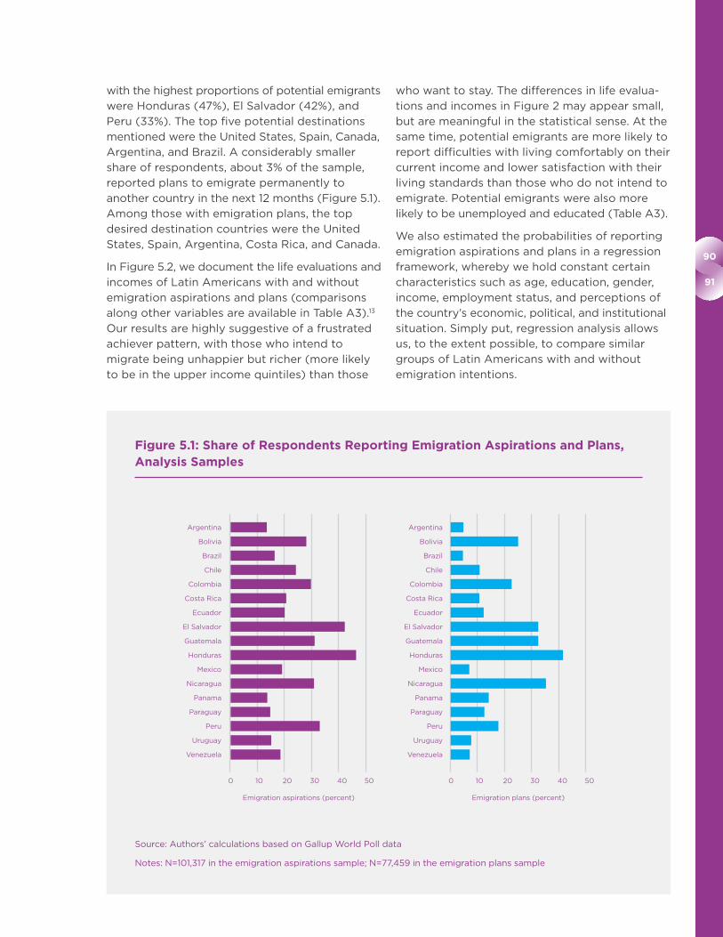
90
91
with the highest proportions of potential emigrants
were Honduras (47%), El Salvador (42%), and
Peru (33%). The top five potential destinations
mentioned were the United States, Spain, Canada,
Argentina, and Brazil. A considerably smaller
share of respondents, about 3% of the sample,
reported plans to emigrate permanently to
another country in the next 12 months (Figure 5.1).
Among those with emigration plans, the top
desired destination countries were the United
States, Spain, Argentina, Costa Rica, and Canada.
In Figure 5.2, we document the life evaluations and
incomes of Latin Americans with and without
emigration aspirations and plans (comparisons
along other variables are available in Table A3).13
Our results are highly suggestive of a frustrated
achiever pattern, with those who intend to
migrate being unhappier but richer (more likely
to be in the upper income quintiles) than those
who want to stay. The differences in life evalua-
tions and incomes in Figure 2 may appear small,
but are meaningful in the statistical sense. At the
same time, potential emigrants are more likely to
report difficulties with living comfortably on their
current income and lower satisfaction with their
living standards than those who do not intend to
emigrate. Potential emigrants were also more
likely to be unemployed and educated (Table A3).
We also estimated the probabilities of reporting
emigration aspirations and plans in a regression
framework, whereby we hold constant certain
characteristics such as age, education, gender,
income, employment status, and perceptions of
the country’s economic, political, and institutional
situation. Simply put, regression analysis allows
us, to the extent possible, to compare similar
groups of Latin Americans with and without
emigration intentions.
Figure 5.1: Share of Respondents Reporting Emigration Aspirations and Plans, Analysis Samples
Source: Authors’ calculations based on Gallup World Poll data
Notes: N=101,317 in the emigration aspirations sample; N=77,459 in the emigration plans sample
Argentina
Bolivia
Brazil
Chile
Colombia
Costa Rica
Ecuador
El Salvador
Guatemala
Honduras
Mexico
Nicaragua
Panama
Paraguay
Peru
Uruguay
Venezuela
Emigration aspirations (percent) Emigration plans (percent)
Argentina
Bolivia
Brazil
Chile
Colombia
Costa Rica
Ecuador
El Salvador
Guatemala
Honduras
Mexico
Nicaragua
Panama
Paraguay
Peru
Uruguay
Venezuela
0 10 20 30 40 50 0 10 20 30 40 50

World Happiness Report 2018
These regression results (shown in Table A4)
confirm the frustrated achiever story. First,
emigration aspirations and plans for Latin
American respondents decrease as happiness
(evaluative and hedonic well-being) increases.
Simply put, the happier people are, the less likely
they are to want to leave their homes and emigrate
abroad. A one-unit increase in evaluative well-
being is associated with a 0.3 percentage point
decline in the probability of reporting emigration
aspirations and a 0.1 percentage point decline
in the probability of reporting emigration plans.
Having smiled the day before is also associated
with a lower chance of reporting emigration
aspirations and plans.
Figure 5.3 displays the key findings from the
regression analyses. The predicted probability of
having emigration aspirations is 27% for the least
happy respondents (whose best possible life
evaluation scores are at 0), while it is 23% for the
happiest respondents (whose life evaluations are
at 10), a difference of 4 percentage points.
Another way to put these effects in perspective is
to look at the difference in predicted emigration
intentions of those at the bottom quartile and
Figure 5.2: Average Life Evaluations and Percent of Respondents in Upper Income Quintiles, Analysis Samples
Source: Authors’ calculations based on Gallup World Poll data
Notes: N=101,317 in the emigration aspirations sample; N=77,459 in the emigration plans sample. See Table A3 for more details. Percent high-income refers to the “share of respondents in the top two income quintiles.” The differences in means between all groups are statistically significant. The p-value of the t-test of equality of means between those with and without emigration intentions (top left panel) is 0.000 (t-stat=12.2). The p-value of the t-test of the equality of means (percent high-income) between those with and without emigration intentions (bottom left panel) is 0.000 (t-stat=12.9). The p-value of the t-test of the equality of means (percent high-income) between those with and without emigration plans (bottom right panel) is 0.000 (t-stat=5.2). The p-value of the t-test of the equality of means (life evaluations) between those with and without emigration plans (top right panel) is 0.000 (t-stat=7.1).
7
6
5
4
3
2
1
50
40
30
20
10
Avera
ge life e
valu
ati
on
s (0
-10
)P
erc
en
t
intent no intent
intent no intent
plan no plan
plan no plan
6.13
43.92
6.04
47.92
6.35
39.22
6.31
40.23
Average life evaluations
Percent high-income
Average life evaluations
Percent high-income

92
93
top quartile of the life evaluations distribution.
Specifically, the emigration probability for those
at the 25th percentile of the happiness distribution
(life evaluation=5) is 25.5%, while for those at the
75th percentile of happiness distribution (life
evaluation score=8) it is 24.6%, a difference of
just 1 percentage point. The difference in the
predicted emigration aspirations for respondents
reporting no smiling (a measure of hedonic
well-being/affect) and those who do is about
2.4 percentage points, meanwhile (see Table A4).
The predicted probability of having emigration
plans is much lower than that for having
emigration aspirations, with the difference
between the probability of reporting emigration
plans being 3.3% for the least happy Latin
Americans in the sample and 2.6% for the
happiest ones. These results are in line with the
findings in other studies on Latin American
emigration intentions.14
Further interesting findings emerge from the
analyses (Table A4). For example, as in other
studies,15 we document that rich individuals are
more likely to express emigration aspirations
compared to poorer individuals within the same
Latin American country. At the same time, those
who find it difficult to get by with their current
income are more likely to want to emigrate than
those who live comfortably with their means.
This reflects that income aspirations matter as
much as current conditions for the emigration
decision. When it comes to the probability of
having concrete emigration plans, however, the
relatively rich and the poor do not differ from
each other.
Figure 5.3: Emigration Aspirations and Plans, Adjusted Predictions with 95% Confidence Intervals
Source: Authors’ calculations based on Gallup World Poll data
Notes: N=101,317 in the emigration aspirations sample; N=77,459 in the emigration plans sample

World Happiness Report 2018
Emigration aspirations and plans also vary
according to how Latin Americans in our sample
perceive their economic mobility. Those who
reported no change in their economic situation
are less likely to have emigration aspirations and
plans compared with those who report that their
economic situation has improved (again reflecting
differences in aspirations). Individuals who report
worsening economic mobility are even more
likely than those reporting economic improvement
to want to move abroad.
There are some additional findings (shown in
Table A4), which are highly intuitive – the more
educated, the unemployed, those living in urban
areas, those with networks abroad, and those
reporting that corruption is present in government
and in business are more likely to want to move.16
The old, females, the married, and those who are
satisfied with institutions and their freedom, as
well as those who have social support, are less
likely to want to move. Respondents experiencing
physical pain are also more likely to want to
emigrate, while household size does not seem
to make a difference for emigration aspirations
and plans.17
We next look at how important different
circumstances are in explaining emigration
intentions and plans.18 Specifically, we show in
Table A4 whether each variable in our analysis
is positively or negatively associated with
emigration intentions and plans, and we here
examine its explanatory power (relative weight
or statistical importance) for the overall
variation in emigration intentions and plans.
Figure 5.4 shows that socio-economic variables
(such as age, marital status, gender, education),
country of origin, and year trends are by far the
biggest predictors of emigration aspirations.
Having a network of contacts abroad is also
a pivotal determinant of potential emigration,
accounting for almost half of the explained
variation in emigration plans, and 16% in
emigration aspirations. At the same time,
subjective well-being is a relatively weak
Figure 5.4: Relative Contribution of Explanatory Variables to Overall Variation in Emigration Aspirations and Plans (Percent Contribution to Pseudo R2)
Source: Authors’ calculations based on Gallup World Poll data
Notes: Based on Shapley-based variance decompositions. Pseudo R2=0.14
Aspirations Plans
Socio-Demographics
Country and year dummies
Network
Institutions
Income and mobility
Health
Freedom
Life evaluations
Social support
0.0 10.0 20.0 30.0 40.0 50.0
40.1
26.3
15.8
47.7
7.8
6.0
19.9
11.4
12.3
5.5
1.0
1.0
1.2
0.6
1.6
0.8
0.5
0.7
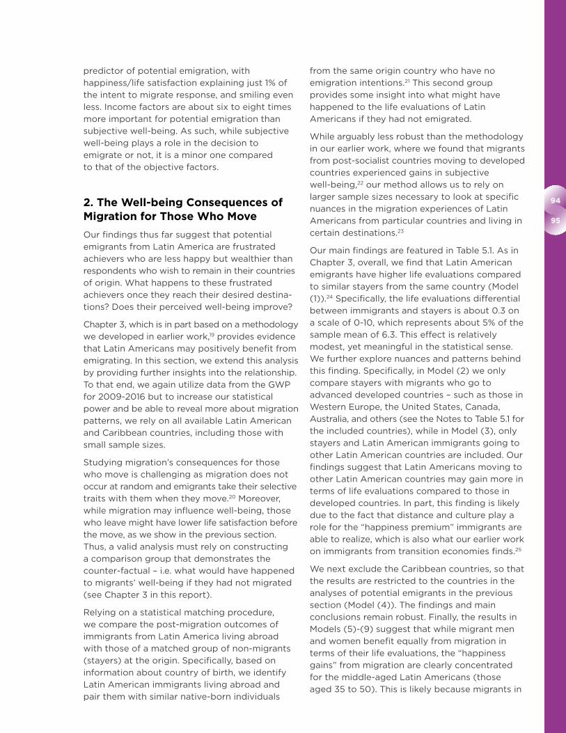
94
95
predictor of potential emigration, with
happiness/life satisfaction explaining just 1% of
the intent to migrate response, and smiling even
less. Income factors are about six to eight times
more important for potential emigration than
subjective well-being. As such, while subjective
well-being plays a role in the decision to
emigrate or not, it is a minor one compared
to that of the objective factors.
2. The Well-being Consequences of Migration for Those Who Move
Our findings thus far suggest that potential
emigrants from Latin America are frustrated
achievers who are less happy but wealthier than
respondents who wish to remain in their countries
of origin. What happens to these frustrated
achievers once they reach their desired destina-
tions? Does their perceived well-being improve?
Chapter 3, which is in part based on a methodology
we developed in earlier work,19 provides evidence
that Latin Americans may positively benefit from
emigrating. In this section, we extend this analysis
by providing further insights into the relationship.
To that end, we again utilize data from the GWP
for 2009-2016 but to increase our statistical
power and be able to reveal more about migration
patterns, we rely on all available Latin American
and Caribbean countries, including those with
small sample sizes.
Studying migration’s consequences for those
who move is challenging as migration does not
occur at random and emigrants take their selective
traits with them when they move.20 Moreover,
while migration may influence well-being, those
who leave might have lower life satisfaction before
the move, as we show in the previous section.
Thus, a valid analysis must rely on constructing
a comparison group that demonstrates the
counter-factual – i.e. what would have happened
to migrants’ well-being if they had not migrated
(see Chapter 3 in this report).
Relying on a statistical matching procedure,
we compare the post-migration outcomes of
immigrants from Latin America living abroad
with those of a matched group of non-migrants
(stayers) at the origin. Specifically, based on
information about country of birth, we identify
Latin American immigrants living abroad and
pair them with similar native-born individuals
from the same origin country who have no
emigration intentions.21 This second group
provides some insight into what might have
happened to the life evaluations of Latin
Americans if they had not emigrated.
While arguably less robust than the methodology
in our earlier work, where we found that migrants
from post-socialist countries moving to developed
countries experienced gains in subjective
well-being,22 our method allows us to rely on
larger sample sizes necessary to look at specific
nuances in the migration experiences of Latin
Americans from particular countries and living in
certain destinations.23
Our main findings are featured in Table 5.1. As in
Chapter 3, overall, we find that Latin American
emigrants have higher life evaluations compared
to similar stayers from the same country (Model
(1)).24 Specifically, the life evaluations differential
between immigrants and stayers is about 0.3 on
a scale of 0-10, which represents about 5% of the
sample mean of 6.3. This effect is relatively
modest, yet meaningful in the statistical sense.
We further explore nuances and patterns behind
this finding. Specifically, in Model (2) we only
compare stayers with migrants who go to
advanced developed countries – such as those in
Western Europe, the United States, Canada,
Australia, and others (see the Notes to Table 5.1 for
the included countries), while in Model (3), only
stayers and Latin American immigrants going to
other Latin American countries are included. Our
findings suggest that Latin Americans moving to
other Latin American countries may gain more in
terms of life evaluations compared to those in
developed countries. In part, this finding is likely
due to the fact that distance and culture play a
role for the “happiness premium” immigrants are
able to realize, which is also what our earlier work
on immigrants from transition economies finds.25
We next exclude the Caribbean countries, so that
the results are restricted to the countries in the
analyses of potential emigrants in the previous
section (Model (4)). The findings and main
conclusions remain robust. Finally, the results in
Models (5)-(9) suggest that while migrant men
and women benefit equally from migration in
terms of their life evaluations, the “happiness
gains” from migration are clearly concentrated
for the middle-aged Latin Americans (those
aged 35 to 50). This is likely because migrants in

World Happiness Report 2018
this age group are in their prime working years,
whereby their chances of income and opportunity
gains are highest, while younger and in particular
older migrants may benefit more from being
near their families, and have less to trade off in
terms of income gains.
We next turn our attention to the experiences of
migrants from the sending countries with at least
90 migrants. These results should be interpreted
with caution due to the small sample sizes. Table
5.2 reveals that not all migrants uniformly gain
from emigrating. For example, the post-migration
life evaluation levels of Venezuelans, Mexicans,
Argentinians, Bolivians, and Chileans are, on
average, indistinguishable from those of their
compatriots who did not emigrate. Moreover,
Brazilian immigrants, whose top three destination
countries are Portugal, Paraguay, and Uruguay,
may even incur life evaluation losses compared
to comparable non-migrant Brazilians at the
origin. At the same time, Colombians, Nicaraguans,
Paraguayans, and Peruvians living abroad are
happier than their stayer counterparts. It is
difficult to explain the differences across so many
different countries. It is more intuitive for some,
such as Nicaragua, Colombia, and Paraguay,
where migrants are leaving either civil violence
or generally poor governance behind, than for
others. In the specific case of Venezuela, mean-
while, it is plausible that many migrations were
not desired paths, but rather an escape from an
atmosphere of rapidly deteriorating political
freedom and economic stability.
Finally, Table 5.3 offers some insights into the
happiness differential between migrants and
stayers at particular destination countries.
Immigrants from Latin American countries living in
Spain, Costa Rica, and Argentina, may be better off
in terms of happiness compared to their counter-
parts in the origin countries. Yet immigrants in the
United States, Panama, and Portugal may not be
happier after migrating, though the non-statistically
significant findings may be due to the small
sample sizes. Given the largest immigrant group
in the United States in our matched sample are
Mexicans, the nil happiness gains may also reflect
Table 5.1: Difference in Life Evaluation Levels Between Latin American Migrants and Matched Stayers
(1) (2) (3) (4) (5) (6) (7) (8) (9)
Overall Advanced countries
destinations
LAC destinations
Restricted sample
Females Males Age 34 and younger
Ages 35-50 50 and older
Life evaluations difference
0.316*** 0.171* 0.481*** 0.287*** 0.267*** 0.238** 0.145 0.473*** 0.171
(0.070) (0.096) (0.099) (0.071) (0.090) (0.109) (0.109) (0.120) (0.133)
N 4,262 1,722 2,426 4,006 2,546 1,716 1,610 1,328 1,324
Adj. R2 0.065 0.069 0.050 0.060 0.063 0.063 0.041 0.076 0.063
Source: Authors’ calculations based on Gallup World Poll data
Notes: Robust standard errors in parentheses. The differences are based on OLS regressions applied after statistical matching. All estimates are adjusted for the pre-treatment covariates (age groups, gender, education levels, country of origin, and year of interview). Column (1) shows the estimates for the full matched sample for all matched Latin American and Caribbean countries. The advanced country destinations in (2) are based on all available countries from the list in Nikolova and Graham (2015a) and include: United States, United Kingdom, France, Germany, The Netherlands, Belgium, Spain, Italy, Sweden, Greece, Denmark, Hong Kong, Japan, Israel, Canada, Australia, New Zealand, South Korea, Austria, Cyprus, Finland, Iceland, Ireland, Luxembourg, Malta, Norway, Portugal, Slovenia, and Switzerland. The LAC destinations in (3) are: Venezuela, Brazil, Mexico, Costa Rica, Argentina, Belize, Bolivia, Chile, Colombia, Dominican Republic, Ecuador, El Salvador, Guatemala Honduras, Nicaragua, Panama, Paraguay, Peru, Puerto Rico, and Uruguay. The restricted sample in (4) includes the following origin countries: Brazil, Mexico, Costa Rica, Argentina, Bolivia, Chile, Colombia, Ecuador, El Salvador, Guatemala, Honduras, Nicaragua, Panama, Paraguay, Peru, and Uruguay. Models (5)-(9) are based on the overall sample, which is split according to the respective socio-demographic characteristic.
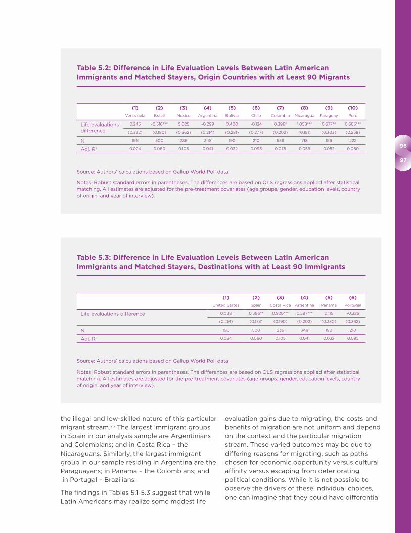
96
97
the illegal and low-skilled nature of this particular
migrant stream.26 The largest immigrant groups
in Spain in our analysis sample are Argentinians
and Colombians; and in Costa Rica – the
Nicaraguans. Similarly, the largest immigrant
group in our sample residing in Argentina are the
Paraguayans; in Panama – the Colombians; and
in Portugal – Brazilians.
The findings in Tables 5.1-5.3 suggest that while
Latin Americans may realize some modest life
evaluation gains due to migrating, the costs and
benefits of migration are not uniform and depend
on the context and the particular migration
stream. These varied outcomes may be due to
differing reasons for migrating, such as paths
chosen for economic opportunity versus cultural
affinity versus escaping from deteriorating
political conditions. While it is not possible to
observe the drivers of these individual choices,
one can imagine that they could have differential
Table 5.2: Difference in Life Evaluation Levels Between Latin American Immigrants and Matched Stayers, Origin Countries with at Least 90 Migrants
(1) (2) (3) (4) (5) (6) (7) (8) (9) (10)
Venezuela Brazil Mexico Argentina Bolivia Chile Colombia Nicaragua Paraguay Peru
Life evaluations difference
0.245 -0.516*** 0.025 -0.299 0.400 -0.124 0.396* 1.058*** 0.677** 0.685***
(0.332) (0.180) (0.262) (0.214) (0.281) (0.277) (0.202) (0.191) (0.303) (0.258)
N 196 500 236 348 190 210 556 718 186 222
Adj. R2 0.024 0.060 0.105 0.041 0.032 0.095 0.078 0.058 0.052 0.060
Source: Authors’ calculations based on Gallup World Poll data
Notes: Robust standard errors in parentheses. The differences are based on OLS regressions applied after statistical matching. All estimates are adjusted for the pre-treatment covariates (age groups, gender, education levels, country of origin, and year of interview).
Table 5.3: Difference in Life Evaluation Levels Between Latin American Immigrants and Matched Stayers, Destinations with at Least 90 Immigrants
(1) (2) (3) (4) (5) (6)
United States Spain Costa Rica Argentina Panama Portugal
Life evaluations difference 0.038 0.396** 0.920*** 0.587*** 0.115 -0.326
(0.291) (0.173) (0.190) (0.202) (0.330) (0.362)
N 196 500 236 348 190 210
Adj. R2 0.024 0.060 0.105 0.041 0.032 0.095
Source: Authors’ calculations based on Gallup World Poll data
Notes: Robust standard errors in parentheses. The differences are based on OLS regressions applied after statistical matching. All estimates are adjusted for the pre-treatment covariates (age groups, gender, education levels, country of origin, and year of interview).
World Happiness Report 2018
effects on subjective well-being outcomes. Our
work comparing the life satisfaction of migrants
from transition countries suggests that migrants
who move to places where it is easy to assimilate
culturally and/or also have the ability to return
home frequently and with ease tend to have
higher gains in subjective well-being than those
who do not.27
3. Emigration’s Consequences for the Well-being of the Family Left Behind at the Origin
Thus far, we have found that potential Latin
American emigrants are frustrated achievers who
may gain in terms of happiness from migrating.
In this section, we examine the well-being of
migrants’ family members left behind in the
countries of origin.
We rely on two questions in the Gallup World
Poll: (i) whether the respondent has family
abroad who left in the last five years and is still
in the destination country and (ii) whether the
respondent’s household receives remittances
(both in kind and monetary) from abroad. All
analyses are for 2009-2010 due to the availability
of the family abroad variable. The Poll included a
question about which country respondents’
relatives are in, and the top locations for Latin
Americans were the U.S., Spain, and Argentina.
We use several outcome variables capturing
evaluative well-being, and positive and negative
hedonic affect.28
Emigration can have conflicting consequences
for the subjective well-being of the left behind.
On the one hand, it may result in negative
emotions due to the pain of separation. On the
other hand, it may also increase psychological
well-being if relatives back home know that
migrants are expanding their opportunities
abroad. Furthermore, remittances should at least
in part compensate for the pain of separation.
For example, remittance receipt is positively
associated with life satisfaction in Latin America,
possibly through increased financial security.29
An additional study documents that migrant and
non-migrant households in Cuenca, Ecuador
experience similar happiness levels, arguing that
remittances compensate migrant households for
the pain of separation and the disruption of
family life.30
About 17% of respondents in our analysis sample
have a family member abroad who emigrated in
the last five years (see Tables A6 and A7 in the
Appendix for information regarding the analysis
sample). The first set of results (Table 5.4)
document the relationship between the
emigration of family members and life evaluations
(See Table A8 for detailed findings).
Our findings suggest a positive relationship
between having family members abroad and life
evaluations, which is independent of remittance
receipt (Table 5.4). Having family abroad corre-
sponds to an average increase in life evaluations
by about 0.10 points (on a 0-10 scale) Models
(1)-(2). This associated influence is substantively
small.31 Next, we net out the influence of the
within-country income quintile of the respondent,
thus comparing the well-being of households
with similar levels of income Models (3)-(6).
Having relatives and friends abroad is still
positively associated with life evaluations.32
We next include variables for financial and living
standard satisfaction and economic mobility,
which are important determinants of the emigration
decision, as shown above (Models (5)-(6) in Table
5.4). Once we control for this perceived economic
status, the positive influence of having relatives
and friends abroad becomes smaller and indistin-
guishable from zero. This suggests that part of
the happiness “premium” for the left behinds
associated with having relatives and friends
abroad stems from the perceived economic
mobility and financial security that comes with it.33
We also examined the relationship between
family members moving abroad and smiling,
stress, and depression (Table A9 in the Appendix).
Having relatives abroad and remittance receipts
have no association with smiling and stress.
There is, however, is a clear relationship with
reporting depression, which is independent of
remittance receipt. Having relatives abroad is
associated with one percentage point increase in
the probability of feeling depressed the previous
day; meanwhile, 13.7% of respondents with family
abroad report depression feelings (Table A7).
This likely reflects the pain of separation, and is
independent of having a social network of family
and friends on whom to rely in times of need.
Additional analyses (not shown) reveal that the
associated increase in depression resulting from
the out-migration of family members also holds

98
99
once we net out the influence of income, financial
and standard of living satisfaction, and economic
mobility perceptions.
Our results are in line with to those in an earlier
study, which looks at out-migration from several
world regions.34 Sub-Saharan Africa is the only
other region displaying a similar statistically
significant relationship between depression and
the out-migration of family members. This very
likely reflects the longer distance and at times
illegal status that emigrants from these two
regions (Latin America and sub-Saharan Africa)
face when they arrive in the U.S. and Europe, and
their related inability to return home frequently.
4. Conclusions
Chapter 6 in this report, as well as our earlier
findings,35 highlight the complex reasons for
Latin Americans’ higher than average well-being
scores. The hedonic dimensions of well-being
play a strong role in this explanation, and likely
reflect cultural traits, such as the high value that
Latins attach to family ties and quality of social
life. Nevertheless, the strong role that learning or
creativity plays in Latins’ well-being goes well
beyond the hedonic or daily dimensions of
well-being and suggests a deeper appreciation
of quality of life in the region. A puzzle, then,
is why there is so much out-migration from
the region.
Our exploration of the reasons for and the
consequences of emigration in this chapter finds
that factors such as income and perceived
mobility lead many Latin Americans to sacrifice
their family and social life at home to seek
opportunities and better life chances abroad.
Those who wish to emigrate are less satisfied
with their lives and their economic situations
than their counterparts who stay behind, and on
average, they realize modest gains in terms of
happiness once they move. While their family
members left in the places of origin realize
Table 5.4: Emigration of Family Members, Remittances, and Life Evaluations
(1) (2) (3) (4) (5) (6)
Life evaluations Life evaluations Life evaluations Life evaluations Life evaluations Life evaluations
Relatives abroad
0.124*** 0.108** 0.085** 0.078* 0.063* 0.058
(0.043) (0.045) (0.039) (0.041) (0.037) (0.039)
Remittances
0.073 0.032 0.025
(0.062) (0.056) (0.054)
Remittance control N Y N Y N Y
Income quintile controls N N Y Y Y Y
Economic mobility, financial
satisfaction, living standard
satisfaction
N N N N Y Y
Country dummies and control
variables
Y Y Y Y Y Y
Observations 23,909 23,909 23,909 23,909 23,909 23,909
Adjusted R2 0.152 0.152 0.163 0.163 0.230 0.230
Source: Authors’ calculations based on Gallup World Poll data
Notes: Robust standard errors are reported in parentheses. All models include controls for social support, age, age squared, gender, marital status, child in the household, household size, education, unemployment status, pain yesterday, health problem, religiosity, freedom, urban location, and a dummy for year 2010. All regressions use the Gallup-provided survey weight. The sample includes Venezuela, Brazil, Mexico, Costa Rica, Argentina, Bolivia, Chile, Colombia, Ecuador, El Salvador, Guatemala, Honduras, Nicaragua, Panama Paraguay, Peru, and Uruguay and excludes the foreign-born in each country of interview.
*** p<0.01, ** p<0.05, * p<0.1
World Happiness Report 2018
modest life evaluation gains and benefit from the
income gains that result from remittances, they
are also more likely to report depression than are
those without family members abroad.
In short, the Latin American happiness “premium”
is not without its own paradoxes – migration
being a primary example. Many individuals choose
to leave to seek opportunities elsewhere, in order
to be better able to provide for themselves and
for the families they leave behind. Some migrant
groups – such as the Paraguayans, Peruvians,
and Nicaraguans abroad – may realize happiness
benefits from emigrating. Yet not all Latin American
migrants become happier by emigrating. Nor are
there net positive effects for the families left
behind, as increases in reported depression often
offset their income gains. This reflects progress
paradoxes that we have identified elsewhere,
meanwhile, where significant income gains can
co-exist with psychological costs.36
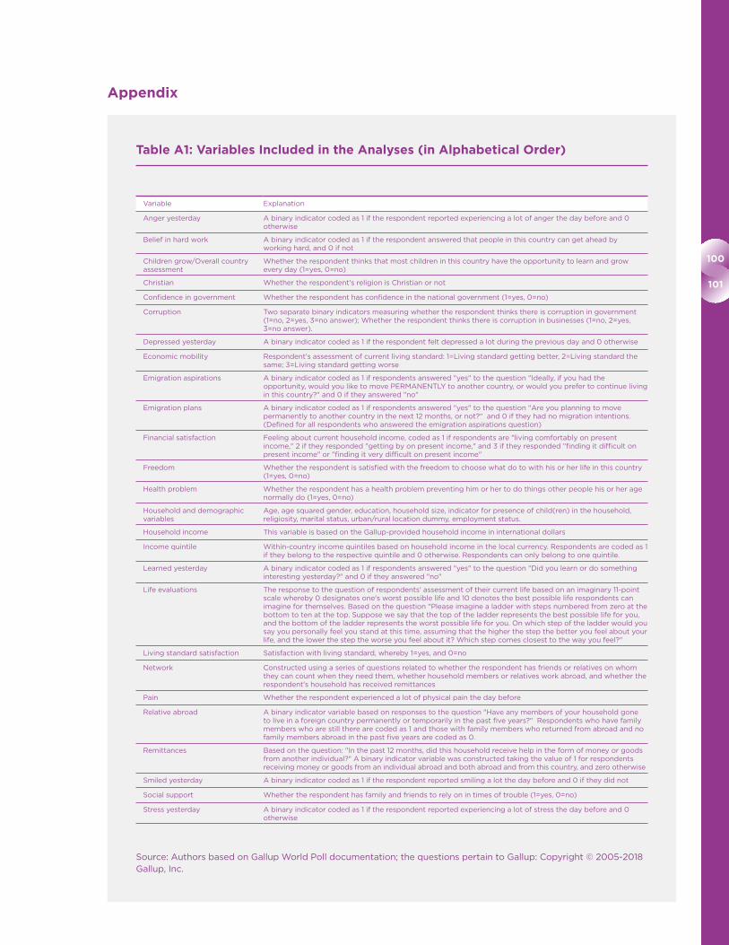
100
101
Table A1: Variables Included in the Analyses (in Alphabetical Order)
Variable Explanation
Anger yesterday A binary indicator coded as 1 if the respondent reported experiencing a lot of anger the day before and 0 otherwise
Belief in hard work A binary indicator coded as 1 if the respondent answered that people in this country can get ahead by working hard, and 0 if not
Children grow/Overall country assessment
Whether the respondent thinks that most children in this country have the opportunity to learn and grow every day (1=yes, 0=no)
Christian Whether the respondent's religion is Christian or not
Confidence in government Whether the respondent has confidence in the national government (1=yes, 0=no)
Corruption Two separate binary indicators measuring whether the respondent thinks there is corruption in government (1=no, 2=yes, 3=no answer); Whether the respondent thinks there is corruption in businesses (1=no, 2=yes, 3=no answer).
Depressed yesterday A binary indicator coded as 1 if the respondent felt depressed a lot during the previous day and 0 otherwise
Economic mobility Respondent's assessment of current living standard: 1=Living standard getting better, 2=Living standard the same; 3=Living standard getting worse
Emigration aspirations A binary indicator coded as 1 if respondents answered "yes" to the question "Ideally, if you had the opportunity, would you like to move PERMANENTLY to another country, or would you prefer to continue living in this country?" and 0 if they answered "no"
Emigration plans A binary indicator coded as 1 if respondents answered "yes" to the question "Are you planning to move permanently to another country in the next 12 months, or not?" and 0 if they had no migration intentions. (Defined for all respondents who answered the emigration aspirations question)
Financial satisfaction Feeling about current household income, coded as 1 if respondents are "living comfortably on present income," 2 if they responded "getting by on present income," and 3 if they responded "finding it difficult on present income" or "finding it very difficult on present income"
Freedom Whether the respondent is satisfied with the freedom to choose what do to with his or her life in this country (1=yes, 0=no)
Health problem Whether the respondent has a health problem preventing him or her to do things other people his or her age normally do (1=yes, 0=no)
Household and demographic variables
Age, age squared gender, education, household size, indicator for presence of child(ren) in the household, religiosity, marital status, urban/rural location dummy, employment status.
Household income This variable is based on the Gallup-provided household income in international dollars
Income quintile Within-country income quintiles based on household income in the local currency. Respondents are coded as 1 if they belong to the respective quintile and 0 otherwise. Respondents can only belong to one quintile.
Learned yesterday A binary indicator coded as 1 if respondents answered "yes" to the question "Did you learn or do something interesting yesterday?" and 0 if they answered "no"
Life evaluations The response to the question of respondents' assessment of their current life based on an imaginary 11-point scale whereby 0 designates one's worst possible life and 10 denotes the best possible life respondents can imagine for themselves. Based on the question "Please imagine a ladder with steps numbered from zero at the bottom to ten at the top. Suppose we say that the top of the ladder represents the best possible life for you, and the bottom of the ladder represents the worst possible life for you. On which step of the ladder would you say you personally feel you stand at this time, assuming that the higher the step the better you feel about your life, and the lower the step the worse you feel about it? Which step comes closest to the way you feel?"
Living standard satisfaction Satisfaction with living standard, whereby 1=yes, and 0=no
Network Constructed using a series of questions related to whether the respondent has friends or relatives on whom they can count when they need them, whether household members or relatives work abroad, and whether the respondent's household has received remittances
Pain Whether the respondent experienced a lot of physical pain the day before
Relative abroad A binary indicator variable based on responses to the question "Have any members of your household gone to live in a foreign country permanently or temporarily in the past five years?" Respondents who have family members who are still there are coded as 1 and those with family members who returned from abroad and no family members abroad in the past five years are coded as 0.
Remittances Based on the question: "In the past 12 months, did this household receive help in the form of money or goods from another individual?" A binary indicator variable was constructed taking the value of 1 for respondents receiving money or goods from an individual abroad and both abroad and from this country, and zero otherwise
Smiled yesterday A binary indicator coded as 1 if the respondent reported smiling a lot the day before and 0 if they did not
Social support Whether the respondent has family and friends to rely on in times of trouble (1=yes, 0=no)
Stress yesterday A binary indicator coded as 1 if the respondent reported experiencing a lot of stress the day before and 0 otherwise
Source: Authors based on Gallup World Poll documentation; the questions pertain to Gallup: Copyright © 2005-2018 Gallup, Inc.
Appendix
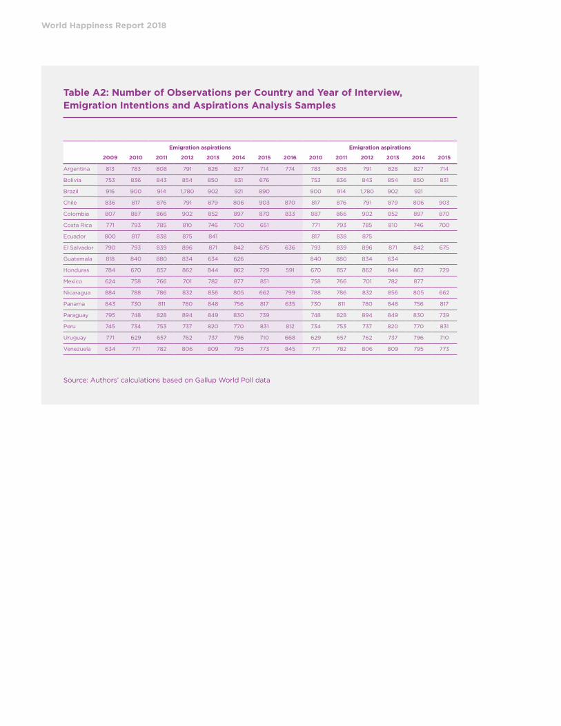
World Happiness Report 2018
Table A2: Number of Observations per Country and Year of Interview, Emigration Intentions and Aspirations Analysis Samples
Emigration aspirations Emigration aspirations
2009 2010 2011 2012 2013 2014 2015 2016 2010 2011 2012 2013 2014 2015
Argentina 813 783 808 791 828 827 714 774 783 808 791 828 827 714
Bolivia 753 836 843 854 850 831 676 753 836 843 854 850 831
Brazil 916 900 914 1,780 902 921 890 900 914 1,780 902 921
Chile 836 817 876 791 879 806 903 870 817 876 791 879 806 903
Colombia 807 887 866 902 852 897 870 833 887 866 902 852 897 870
Costa Rica 771 793 785 810 746 700 651 771 793 785 810 746 700
Ecuador 800 817 838 875 841 817 838 875
El Salvador 790 793 839 896 871 842 675 636 793 839 896 871 842 675
Guatemala 818 840 880 834 634 626 840 880 834 634
Honduras 784 670 857 862 844 862 729 591 670 857 862 844 862 729
Mexico 624 758 766 701 782 877 851 758 766 701 782 877
Nicaragua 884 788 786 832 856 805 662 799 788 786 832 856 805 662
Panama 843 730 811 780 848 756 817 635 730 811 780 848 756 817
Paraguay 795 748 828 894 849 830 739 748 828 894 849 830 739
Peru 745 734 753 737 820 770 831 812 734 753 737 820 770 831
Uruguay 771 629 657 762 737 796 710 668 629 657 762 737 796 710
Venezuela 634 771 782 806 809 795 773 845 771 782 806 809 795 773
Source: Authors’ calculations based on Gallup World Poll data

102
103
Table A3: Selected Summary Statistics for Respondents with Emigration Aspirations and Emigration Plans
No aspirations, N=77,767
Aspirations, N=23,550 No plans, N=75,378 Plans, N=2,081
Variable Mean Std. Dev. Mean Std. Dev. Mean Std. Dev. Mean Std. Dev.
Live evaluations (0-10 scale) 6.349 2.354 6.134 2.420 6.311 2.355 6.038 2.499
Smiled yesterday (1=yes) 0.863 0.344 0.848 0.359 0.862 0.345 0.844 0.363
Within-country income quintiles
Q1 0.213 0.410 0.182 0.386 0.205 0.404 0.167 0.373
Q2 0.201 0.400 0.184 0.388 0.200 0.400 0.174 0.379
Q3 0.194 0.395 0.194 0.396 0.193 0.394 0.179 0.384
Q4 0.190 0.392 0.205 0.404 0.192 0.394 0.203 0.402
Q5 0.202 0.402 0.234 0.423 0.211 0.408 0.276 0.447
Financial satisfaction
Living comfortably on current income 0.147 0.354 0.137 0.344 0.150 0.357 0.163 0.369
Getting by on current income 0.472 0.499 0.432 0.495 0.465 0.499 0.424 0.494
Difficult on current income 0.380 0.485 0.430 0.495 0.385 0.487 0.413 0.493
Living standard satisfaction 0.741 0.438 0.668 0.471 0.734 0.442 0.682 0.466
Economic mobility
Better 0.517 0.500 0.524 0.499 0.527 0.499 0.550 0.498
No change 0.313 0.464 0.250 0.433 0.303 0.459 0.216 0.412
Worse 0.170 0.375 0.227 0.419 0.171 0.376 0.234 0.423
Education
Elementary 0.376 0.485 0.262 0.440 0.354 0.478 0.247 0.431
Secondary 0.513 0.500 0.601 0.490 0.531 0.499 0.565 0.496
Tertiary 0.110 0.313 0.136 0.343 0.115 0.319 0.188 0.391
Unemployed 0.067 0.249 0.113 0.317 0.079 0.269 0.155 0.362
Source: Authors’ calculations based on Gallup World Poll data
Notes: The reported statistics were weighted using the Gallup-provided survey weight. The sample includes Venezuela, Brazil, Mexico, Costa Rica, Argentina, Bolivia, Chile, Colombia, Ecuador, El Salvador, Guatemala, Honduras, Nicaragua, Panama Paraguay, Peru, and Uruguay and excludes the foreign-born in each country of interview. The means of all variables are statistically significantly different from each other at the 5% confidence level or lower. The exceptions are: the proportion of respondents in Q3 for those in the aspirations sample and Q2 in the plans sample.

World Happiness Report 2018
Table A4: Emigration Aspirations and Plans, Logistic Regressions, Average Marginal Effects
(1) (2) (3) (4)
Aspirations Plans Aspirations Plans
Key independent Variable: Life evaluations
Key independent Variable: Smiled yesterday
Subjective well-being -0.003*** -0.001** -0.024*** -0.006***
(0.001) (0.000) (0.004) (0.002)
Within-country income quintiles (Ref: Q1(poorest))
Q2 0.006 0.001 0.005 0.001
(0.005) (0.002) (0.005) (0.002)
Q3 0.011** 0.001 0.010** 0.001
(0.005) (0.002) (0.005) (0.002)
Q4 0.010** -0.001 0.010* -0.001
(0.005) (0.002) (0.005) (0.002)
Q5 0.011** 0.001 0.010* 0.001
(0.005) (0.003) (0.005) (0.003)
Financial satisfaction (Ref: Living comfortably on current income)
Getting by on current income
0.005 -0.001 0.006 -0.001
(0.005) (0.002) (0.005) (0.002)
Difficult on current income
0.029*** 0.000 0.030*** 0.001
(0.005) (0.002) (0.005) (0.002)
Living standard satisfaction -0.044*** -0.004** -0.045*** -0.005**
(0.004) (0.002) (0.004) (0.002)
Economic mobility (Ref: Better)
No change -0.013*** -0.005*** -0.013*** -0.005***
(0.004) (0.002) (0.004) (0.002)
Worse 0.040*** 0.008*** 0.042*** 0.008***
(0.005) (0.002) (0.005) (0.002)
Education (Ref: Elementary)
Secondary 0.029*** 0.003 0.029*** 0.003
(0.004) (0.002) (0.004) (0.002)
Tertiary 0.042*** 0.011*** 0.041*** 0.010***
(0.006) (0.003) (0.006) (0.003)
Unemployed 0.041*** 0.015*** 0.042*** 0.015***
(0.006) (0.003) (0.006) (0.003)
Age -0.004*** 0.001* -0.004*** 0.001*
(0.001) (0.000) (0.001) (0.000)
Age2/100 -0.001* -0.001*** -0.001* -0.001***
(0.001) (0.000) (0.001) (0.000)
Female -0.027*** -0.007*** -0.027*** -0.007***
(0.003) (0.001) (0.003) (0.001)
Married/Partnership -0.039*** -0.010*** -0.039*** -0.010***
(0.003) (0.002) (0.003) (0.002)
Child in household 0.009** 0.000 0.009** 0.000
(0.004) (0.002) (0.004) (0.002)
Household size 0.000 -0.000 0.000 -0.000
(0.001) (0.000) (0.001) (0.000)
Health problem -0.001 0.001 -0.001 0.001
(0.004) (0.002) (0.004) (0.002)
Pain 0.014*** 0.003* 0.012*** 0.003*
(0.003) (0.002) (0.003) (0.002)
Freedom -0.016*** -0.004** -0.016*** -0.004**
(0.004) (0.002) (0.004) (0.002)
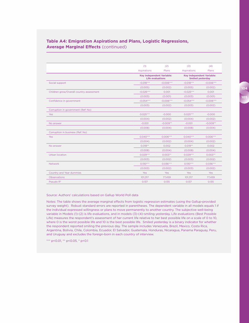
104
105
Table A4: Emigration Aspirations and Plans, Logistic Regressions, Average Marginal Effects (continued)
(1) (2) (3) (4)
Aspirations Plans Aspirations Plans
Key independent Variable: Life evaluations
Key independent Variable: Smiled yesterday
Social support -0.018*** -0.006*** -0.018*** -0.006***
(0.005) (0.002) (0.005) (0.002)
Children grow/Overall country assessment -0.026*** 0.001 -0.025*** 0.001
(0.003) (0.001) (0.003) (0.001)
Confidence in government -0.054*** -0.006*** -0.054*** -0.006***
(0.003) (0.002) (0.003) (0.002)
Corruption in government (Ref: No)
Yes 0.025*** -0.000 0.025*** -0.000
(0.004) (0.002) (0.004) (0.002)
No answer -0.001 -0.009** -0.001 -0.009**
(0.008) (0.004) (0.008) (0.004)
Corruption in business (Ref: No)
Yes 0.040*** 0.006*** 0.040*** 0.006***
(0.004) (0.002) (0.004) (0.002)
No answer 0.018** 0.002 0.019** 0.002
(0.008) (0.004) (0.008) (0.004)
Urban location 0.029*** 0.003** 0.029*** 0.003**
(0.003) (0.002) (0.003) (0.002)
Network 0.130*** 0.036*** 0.130*** 0.036***
(0.003) (0.002) (0.003) (0.002)
Country and Year dummies Yes Yes Yes Yes
Observations 101,317 77,459 101,317 77,459
Pseudo R2 0.137 0.135 0.137 0.135
Source: Authors’ calculations based on Gallup World Poll data
Notes: The table shows the average marginal effects from logistic regression estimates (using the Gallup-provided survey weight). Robust standard errors are reported in parentheses. The dependent variable in all models equals 1 if the individual expressed willingness or plans to move permanently to another country. The subjective well-being variable in Models (1)-(2) is life evaluations, and in models (3)-(4)-smiling yesterday. Life evaluations (Best Possible Life) measures the respondent’s assessment of her current life relative to her best possible life on a scale of 0 to 10, where 0 is the worst possible life and 10 is the best possible life. Smiled yesterday is a binary indicator for whether the respondent reported smiling the previous day. The sample includes Venezuela, Brazil, Mexico, Costa Rica, Argentina, Bolivia, Chile, Colombia, Ecuador, El Salvador, Guatemala, Honduras, Nicaragua, Panama Paraguay, Peru, and Uruguay and excludes the foreign-born in each country of interview.
*** p<0.01, ** p<0.05, * p<0.1

World Happiness Report 2018
Table A5: Summary Statistics, Latin American Immigrants and Stayers, Matched Sample
Immigrants, N=2,131 Stayers, N=2,131
Variable Mean Std. Dev. Mean Std. Dev.
Age 41.968 16.166 41.888 16.065
Female 0.597 0.491 0.597 0.491
Education
Elementary 0.283 0.451 0.283 0.451
Secondary 0.555 0.497 0.555 0.497
Tertiary 0.162 0.368 0.162 0.368
Country of birth
Venezuela 0.046 0.210 0.046 0.210
Brazil 0.117 0.322 0.117 0.322
Mexico 0.055 0.229 0.055 0.229
Costa Rica 0.009 0.096 0.009 0.096
Argentina 0.082 0.274 0.082 0.274
Bolivia 0.045 0.206 0.045 0.206
Chile 0.049 0.216 0.049 0.216
Colombia 0.130 0.337 0.130 0.337
Dominican Republic 0.028 0.165 0.028 0.165
Ecuador 0.029 0.168 0.029 0.168
El Salvador 0.030 0.169 0.030 0.169
Guatemala 0.034 0.182 0.034 0.182
Haiti 0.023 0.148 0.023 0.148
Honduras 0.017 0.131 0.017 0.131
Jamaica 0.003 0.057 0.003 0.057
Nicaragua 0.168 0.374 0.168 0.374
Panama 0.007 0.084 0.007 0.084
Paraguay 0.044 0.204 0.044 0.204
Peru 0.052 0.222 0.052 0.222
Puerto Rico 0.001 0.038 0.001 0.038
Suriname 0.004 0.061 0.004 0.061
Trinidad and Tobago 0.001 0.031 0.001 0.031
Uruguay 0.024 0.154 0.024 0.154
Survey year
2009 0.105 0.306 0.105 0.306
2010 0.115 0.320 0.115 0.320
2011 0.113 0.317 0.113 0.317
2012 0.129 0.335 0.129 0.335
2013 0.091 0.287 0.091 0.287
2014 0.179 0.384 0.179 0.384
2015 0.132 0.338 0.132 0.338
2016 0.137 0.343 0.137 0.343
Source: Authors’ calculations based on Gallup World Poll data
Notes: The table shows the means and standard deviations of the analysis samples after matching - the means and standard deviations are (almost) identical for both groups due to the exact matching technique we applied.
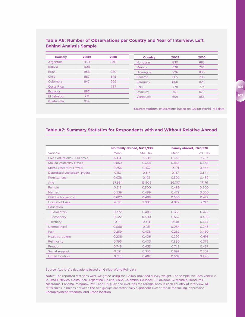
106
107
Table A6: Number of Observations per Country and Year of Interview, Left Behind Analysis Sample
Country 2009 2010
Argentina 860 830
Bolivia 808
Brazil 958 980
Chile 887 875
Colombia 847 929
Costa Rica 797
Ecuador 887
El Salvador 771
Guatemala 834
Country 2009 2010
Honduras 830 683
Mexico 638 793
Nicaragua 926 836
Panama 865 786
Paraguay 860 823
Peru 778 773
Uruguay 821 679
Venezuela 699 856
Table A7: Summary Statistics for Respondents with and Without Relative Abroad
No family abroad, N=19,933 Family abroad, N=3,976
Variable Mean Std. Dev. Mean Std. Dev.
Live evaluations (0-10 scale) 6.414 2.305 6.336 2.287
Smiled yesterday (1=yes) 0.859 0.348 0.868 0.338
Stress yesterday (1=yes) 0.256 0.437 0.271 0.444
Depressed yesterday (1=yes) 0.113 0.317 0.137 0.344
Remittances 0.038 0.192 0.302 0.459
Age 37.994 16.905 36.001 17.176
Female 0.516 0.500 0.489 0.500
Married 0.539 0.499 0.479 0.500
Child in household 0.607 0.488 0.650 0.477
Household size 4.691 2.083 4.977 2.217
Education
Elementary 0.372 0.483 0.335 0.472
Secondary 0.522 0.500 0.537 0.499
Tertiary 0.111 0.314 0.148 0.355
Unemployed 0.068 0.251 0.064 0.245
Pain 0.259 0.438 0.282 0.450
Health problem 0.208 0.406 0.220 0.414
Religiosity 0.795 0.403 0.830 0.375
Freedom 0.749 0.433 0.742 0.437
Social support 0.871 0.336 0.899 0.302
Urban location 0.615 0.487 0.602 0.490
Source: Authors’ calculations based on Gallup World Poll data
Notes: The reported statistics were weighted using the Gallup-provided survey weight. The sample includes Venezue-la, Brazil, Mexico, Costa Rica, Argentina, Bolivia, Chile, Colombia, Ecuador, El Salvador, Guatemala, Honduras, Nicaragua, Panama Paraguay, Peru, and Uruguay and excludes the foreign-born in each country of interview. All differences in means between the two groups are statistically significant except those for smiling, depression, unemployment, freedom, and urban location.
Source: Authors’ calculations based on Gallup World Poll data

World Happiness Report 2018
Table A8: Emigration of Family Members, Remittances, and Life Evaluations
(1) (2) (3) (4) (5) (6)
Life evaluations Life evaluations Life evaluations Life evaluations Life evaluations Life evaluations
Relatives abroad
0.124*** 0.108** 0.085** 0.078* 0.063* 0.058
(0.043) (0.045) (0.039) (0.041) (0.037) (0.039)
Remittances
0.073 0.032 0.025
(0.062) (0.056) (0.054)
Social support
0.755*** 0.752*** 0.688*** 0.687*** 0.405*** 0.404***
(0.046) (0.046) (0.046) (0.046) (0.044) (0.044)
Within-country income quintiles (Ref: Q1(poorest))
Q2
0.254*** 0.253*** 0.155*** 0.155***
(0.045) (0.046) (0.044) (0.044)
Q3
0.463*** 0.462*** 0.270*** 0.269***
(0.046) (0.046) (0.045) (0.045)
Q4
0.640*** 0.639*** 0.355*** 0.354***
(0.046) (0.046) (0.045) (0.045)
Q5
0.869*** 0.868*** 0.435*** 0.434***
(0.048) (0.048) (0.049) (0.049)
Financial satisfaction (Ref: Living comfortably on current income)
Getting by on current income
-0.336*** -0.336***
(0.040) (0.040)
Difficult on current income
-0.672*** -0.672***
(0.048) (0.048)
Economic mobility (Ref: Better)
No change
-0.307*** -0.307***
(0.031) (0.031)
Worse
-0.925*** -0.925***
(0.046) (0.046)
Living standard satisfaction
0.767*** 0.767***
(0.034) (0.034)
Age
-0.053*** -0.053*** -0.054*** -0.054*** -0.032*** -0.032***
(0.005) (0.005) (0.004) (0.004) (0.004) (0.004)
Age2/100
0.047*** 0.047*** 0.048*** 0.048*** 0.029*** 0.029***
(0.005) (0.005) (0.005) (0.005) (0.004) (0.004)
Female
0.108*** 0.107*** 0.136*** 0.136*** 0.138*** 0.138***
(0.032) (0.032) (0.028) (0.028) (0.027) (0.027)
Married/In partnership
-0.003 -0.002 -0.019 -0.018 -0.028 -0.028
(0.036) (0.036) (0.031) (0.031) (0.030) (0.030)
Child in household
-0.120*** -0.120*** -0.103*** -0.103*** -0.089*** -0.089***
(0.039) (0.039) (0.035) (0.035) (0.033) (0.033)
Household size
-0.016 -0.016 -0.027*** -0.027*** -0.012 -0.012
(0.010) (0.010) (0.009) (0.009) (0.008) (0.008)
Education (Ref: Elementary)
Secondary education
0.445*** 0.444*** 0.285*** 0.284*** 0.249*** 0.249***
(0.041) (0.041) (0.037) (0.037) (0.035) (0.035)
Tertiary education
0.761*** 0.760*** 0.426*** 0.426*** 0.353*** 0.353***
(0.054) (0.054) (0.050) (0.050) (0.048) (0.048)
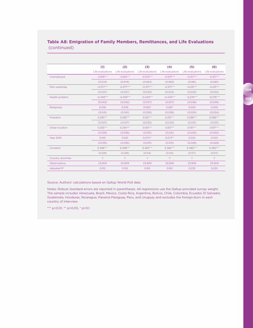
108
109
Table A8: Emigration of Family Members, Remittances, and Life Evaluations (continued)
(1) (2) (3) (4) (5) (6)
Life evaluations Life evaluations Life evaluations Life evaluations Life evaluations Life evaluations
Unemployed
-0.615*** -0.615*** -0.575*** -0.575*** -0.317*** -0.317***
(0.074) (0.074) (0.063) (0.063) (0.061) (0.061)
Pain yesterday
-0.377*** -0.377*** -0.371*** -0.371*** -0.215*** -0.215***
(0.037) (0.037) (0.033) (0.033) (0.032) (0.032)
Health problem
-0.458*** -0.459*** -0.449*** -0.449*** -0.276*** -0.276***
(0.042) (0.042) (0.037) (0.037) (0.036) (0.036)
Religiosity
0.036 0.035 0.062* 0.061* 0.005 0.005
(0.041) (0.041) (0.036) (0.036) (0.034) (0.034)
Freedom
0.295*** 0.295*** 0.251*** 0.251*** 0.086*** 0.086***
(0.037) (0.037) (0.032) (0.032) (0.031) (0.031)
Urban location
0.255*** 0.254*** 0.154*** 0.153*** 0.197*** 0.197***
(0.035) (0.035) (0.031) (0.031) (0.030) (0.030)
Year 2010
0.051 0.051 0.073** 0.073** 0.022 0.022
(0.035) (0.035) (0.031) (0.031) (0.029) (0.029)
Constant
6.498*** 6.498*** 6.382*** 6.382*** 6.480*** 6.480***
(0.129) (0.129) (0.114) (0.114) (0.117) (0.117)
Country dummies Y Y Y Y Y Y
Observations 23,909 23,909 23,909 23,909 23,909 23,909
Adjusted R2 0.152 0.152 0.163 0.163 0.230 0.230
Source: Authors’ calculations based on Gallup World Poll data
Notes: Robust standard errors are reported in parentheses. All regressions use the Gallup-provided survey weight. The sample includes Venezuela, Brazil, Mexico, Costa Rica, Argentina, Bolivia, Chile, Colombia, Ecuador, El Salvador, Guatemala, Honduras, Nicaragua, Panama Paraguay, Peru, and Uruguay and excludes the foreign-born in each country of interview.
*** p<0.01, ** p<0.05, * p<0.1

World Happiness Report 2018
Table A9: Emigration of Family Members, Remittances, Positive and Negative Hedonic Well-Being, Logistic Regressions, Average Marginal Effects
(1) (2) (3) (4) (5) (6)
Smiled yesterday Smiled yesterday Stress yesterday Stress yesterday Depressed yesterday
Depressed yesterday
Relatives abroad
0.008 0.011 0.010 0.006 0.010* 0.011*
(0.007) (0.007) (0.008) (0.009) (0.006) (0.006)
Remittances
-0.014 0.018 -0.003
(0.010) (0.012) (0.008)
Social support
0.064*** 0.064*** -0.052*** -0.053*** -0.054*** -0.054***
(0.008) (0.008) (0.009) (0.009) (0.007) (0.007)
Age
-0.004*** -0.004*** 0.010*** 0.010*** 0.004*** 0.004***
(0.001) (0.001) (0.001) (0.001) (0.001) (0.001)
Age2/100
0.004*** 0.004*** -0.012*** -0.012*** -0.004*** -0.004***
(0.001) (0.001) (0.001) (0.001) (0.001) (0.001)
Female
-0.009* -0.009* 0.036*** 0.036*** 0.026*** 0.026***
(0.005) (0.005) (0.006) (0.006) (0.005) (0.005)
Married/In partnership
0.008 0.008 0.000 0.000 -0.016*** -0.016***
(0.006) (0.006) (0.007) (0.007) (0.005) (0.005)
Child in household
-0.005 -0.005 0.012 0.012 0.009 0.009
(0.006) (0.006) (0.008) (0.008) (0.006) (0.006)
Household size
0.001 0.001 0.001 0.001 -0.001 -0.001
(0.002) (0.002) (0.002) (0.002) (0.001) (0.001)
Education (Ref: Elementary)
Secondary education
0.008 0.008 0.022*** 0.022*** -0.013** -0.013**
(0.006) (0.006) (0.007) (0.007) (0.006) (0.006)
Tertiary education
0.014 0.014 0.029*** 0.028** -0.043*** -0.043***
(0.009) (0.009) (0.011) (0.011) (0.007) (0.007)
Unemployed
-0.023** -0.023** 0.016 0.016 0.059*** 0.059***
(0.011) (0.011) (0.013) (0.013) (0.011) (0.011)
Pain yesterday
-0.094*** -0.094*** 0.243*** 0.243*** 0.136*** 0.136***
(0.007) (0.007) (0.008) (0.008) (0.006) (0.006)
Health problem
-0.028*** -0.028*** 0.068*** 0.068*** 0.063*** 0.063***
(0.007) (0.007) (0.008) (0.008) (0.006) (0.006)
Religiosity
0.036*** 0.036*** -0.006 -0.006 0.002 0.002
(0.007) (0.007) (0.008) (0.008) (0.006) (0.006)
Freedom
0.043*** 0.043*** -0.052*** -0.052*** -0.023*** -0.023***
(0.006) (0.006) (0.007) (0.007) (0.005) (0.005)
Urban location
0.004 0.004 0.042*** 0.042*** 0.010** 0.010**
(0.006) (0.006) (0.007) (0.007) (0.005) (0.005)
Year 2010
0.009* 0.009* -0.009 -0.009 -0.009* -0.009*
(0.005) (0.005) (0.007) (0.007) (0.005) (0.005)
Country dummies Y Y Y Y Y Y
Observations 23,909 23,909 23,909 23,909 23,909 23,909
Pseudo R2 0.054 0.0541 0.096 0.096 0.137 0.137

110
111
Table A9: Emigration of Family Members, Remittances, Positive and Negative Hedonic Well-Being, Logistic Regressions, Average Marginal Effects (continued)
Source: Authors’ calculations based on Gallup World Poll data
Notes: The table shows the average marginal effects from logistic regression estimates (using the Gallup-provided survey weight). Robust standard errors are reported in parentheses. The dependent variable in all models equals 1 if the individual experienced the emotion the day before (smiling in Models (1)-(2), stress in Models (3)-(4), or depres-sion in Models (5)-(6)). The sample includes Venezuela, Brazil, Mexico, Costa Rica, Argentina, Bolivia, Chile, Colombia, Ecuador, El Salvador, Guatemala, Honduras, Nicaragua, Panama Paraguay, Peru, and Uruguay and excludes the foreign-born in each country of interview.
*** p<0.01, ** p<0.05, * p<0.1

World Happiness Report 2018
Endnotes
1 Ivlevs et al. (2016), Nikolova & Graham (2015a, 2015b).
2 The GWP is an annual survey fielded in about 160 countries worldwide, and is representative of each country’s civilian population aged 15 and older, and more than 99% world’s adult population. Here we provide insights for these questions using the latest available data for Latin America in the Poll. Since key variables for our analyses such as income and employment status are available from 2009 onwards, our analyses focus on the years 2009-2016 and cover the following Latin American countries: Argentina, Bolivia, Brazil, Chile, Colombia, Costa Rica, Ecuador, El Salvador, Guatemala, Honduras, Mexico, Nicaragua, Panama, Paraguay, Peru, Uruguay, Venezuela. As they are geographically and culturally distinct from the Latin American countries, we exclude the Caribbean nations (Cuba, the Dominican Republic, Haiti, Jamaica, Trinidad and Tobago, and Puerto Rico). Due to the small sample size of about 500 respondents – polled only once – we also exclude Suriname and Belize. Graham is a Senior Scientist at Gallup and Nikolova a collaborator and, as such, have access to the data.
3 One notable exception is a recent study of return migration to rural areas in Peru conducted by Richard Webb (2013). Webb highlights the important role of improved transporta-tion infrastructure and access to technology (cell phones in particular) in spurring rural residents to return to rural towns and villages to start small businesses. While there are likely other countries that display these trends, we do not have sufficient data, either on return migration or on well-being, to take this topic on.
4 The emigration plans variable is defined for all respondents who answered the emigration aspirations/intentions question. The emigration plans question was not asked in 2009 and 2016.
5 Creighton (2013), Simmons (1985), van Dalen & Henkens (2008, 2013)
6 Massey et al. (1993), Sjaastad (1962)
7 Hanson (2010)
8 Ivlevs (2014)
9 Chindarkar (2014), Graham and Markowitz (2011)
10 Graham and Pettinato (2002)
11 Graham and Markowitz (2011)
12 Similarly, again relying on Latinobarometro data, Chindarkar (2014) shows that life satisfaction is also associated with emigration intentions. Respondents with life satisfaction scores of 3 and 4 (on a 1-4 scale) were two to four percentage points less likely to express emigration intentions.
13 The sample sizes for each country and year are in Table A2 in the Appendix.
14 Graham and Markowitz (2011), Chindarkar (2014)
15 Manchin & Orazbayev (2015)
16 These findings are corroborated by some earlier work by the Gallup Organization and the IOM. See Esipova, Ray, and Pugliese (2011).
17 Our results should be interpreted as conditional correlations rather than as causal estimates, due to a number of methodological and data issues – in particular the cross-sectional nature (see Ivlevs (2014) for a discussion of the methodological challenges).
18 We rely on Shapley-based decomposition, which splits the goodness of fit statistic (i.e., the pseudo R2 in this case) into the relative percentage contributions of each included independent variable (Israeli, 2007; Shorrocks, 2013). To conduct the decompositions, we relied on Stata’s user-written command shapley2 (Juarez, 2012). The pseudo R2 value shows that we were only able to explain about 14% of the variation in emigration aspirations and plans using the included variables in the model.
19 Nikolova and Graham (2015a); see also Esipova, Ray, and Pugliese (2011).
20 By “selective traits,” we mean characteristics such as ability, risk preferences, and aspirations. See Chapter 3 in this report and Nikolova (2015) for the associated challenges of measuring migration’s subjective well-being consequences.
21 We used one-to-one nearest neighbor matching without replacement with a caliper (i.e., maximum allowable distance between the propensity scores) of 0.01. Our matching covariates include age group indicators, as well as gender, country of origin, year of interview, and education. Specifically, we applied exact matching. We excluded income and employment status from the matching covariates as these variables may be influenced by migration itself (see Nikolova and Graham (2015a)). Next, we checked whether on average, the matching covariates are balanced for the migrants and stayers (i.e., whether the means are statistically indistinguishable from zero) and our checks indicate that covariance balance is achieved. Summary statistics are available in Table A5. Finally, we kept the pairs of immigrants and matched stayers that were on the common support. We ran OLS regressions with the matched sample whereby the dependent variable is life evaluations, the focal independent variable is whether the immigrant is a migrant or a stayer. We also include the matching covariates for precision.
22 Nikolova and Graham (2015a)
23 The matched sample is representative of the birth countries and destination countries of all Latin-American immigrant respondents in the GWP.
24 Our findings are very similar to yet slightly different from those in Chapter 3 due to the differences in methodology. Our findings also differ from those in Stillman et al. (2015) who document that migration from Tonga to New Zealand lowers movers’ hedonic well-being despite improvements in income, mental well-being, and income adequacy perceptions. The differences with Stillman et al. (2015) are likely due to differences in the origin and destination countries and in methodology.

112
113
25 In Nikolova and Graham (2015a), we show that migrants from transition economies realize happiness, income, and freedom perception gains when they move to developed countries. In that paper, we also present suggestive evidence that distance (cultural as well as physical) is negatively correlated with the life evaluations of the immigrants. We also document a North/South difference in terms of well-being gains (with migrants living in advanced western societies gaining more than those living in the South i.e., Italy, Greece, Portugal, Spain) and post-socialist migrants moving to the “old” EU gaining the most in terms of both happiness and income.
26 It is important to note that Gallup does not collect data on the legal status of immigrants. This is our interpretation of the results.
27 Nikolova and Graham (2015a)
28 Our methodology is similar to that in Ivlevs et al. (2016).
29 Cárdenas et al. (2009)
30 Borraz et al. (2010)
31 Evaluated at the sample mean, the coefficient estimate is about 1.5 percent.
32 These findings resonate with those for Latin America and the Caribbean in Ivlevs et al. (2016). The main difference is that in Ivlevs et al., in addition to having relatives and friends abroad, the remittance variable is also positive and statistically significant, likely due to the inclusion of the poorer Caribbean countries, whereby remittances enhance the life evaluation effects of being a migrant-sending household.
33 Our findings corroborate those in Nobles et al. (2015) and Marchetti-Mercer (2012), who find a negative relationship between the emigration of household members and the mental well-being of those left behind in Mexico and South Africa. They also echo our previous finding that the emigration of family members is associated with higher levels of depression in more unequal countries (and the world’s most unequal countries are in sub-Saharan Africa and Latin America) (see Ivlevs et al. (2016)).
34 Ivlevs et al. (2016)
35 Graham and Nikolova (2015)
36 Graham & Pettinato (2002), Graham et al. (2017)

World Happiness Report 2018
References
Borraz, F., Pozo, S., & Rossi, M. (2010). And what about the family back home? International migration and happiness in Cuenca, Ecuador. Journal of Business Strategies, 27(1), 7.
Cárdenas, M., Di Maro, V., & Sorkin, I. (2009). Migration and life satisfaction: Evidence from Latin America. Journal of Business Strategies, 26(1), 9-33.
Chindarkar, N. (2014). Is Subjective well-being of concern to potential migrants from Latin America? Social Indicators Research, 115(1), 159-182.
Creighton, M. J. (2013). The role of aspirations in domestic and international migration. The Social Science Journal, 50(1), 79-88.
Esipova, N., Ray, J., and Pugliese, A. (2011). “Gallup World Poll: The Many Faces of Global Migration”, IOM Migration Series, International Organization for Migration; Geneva.
Fields, G. S. (2003). Accounting for income inequality and its change: A new method, with application to the distribution of earnings in the United States. Research in Labor Economics, 22, 1-38.
Fields, G. S. (2004). Regression-based decompositions: A new tool for managerial decision-making. Department of Labor Economics, Cornell University, 1-41.
Graham, C., & Pettinato, S. (2002). Frustrated achievers: winners, losers and subjective well-being in new market economies. The Journal of Development Studies, 38(4), 100-140.
Graham, C., & Nikolova, M. (2015). Bentham or Aristotle in the development process? An empirical investigation of capabilities and subjective well-being. World Development, 68, 163-179.
Graham, C., Zhou, S., & Zhang, J. (2017). Happiness and health in China: The paradox of progress. World development, 96(Supplement C), 231-244.
Hanson, G. H. (2010). International migration and the developing world. In D. Rodrik & M. Rosenzweig (Eds.), Handbook of Development Economics (Vol. 5, pp. 4363-4414).
Israeli, O. (2007). A Shapley-based decomposition of the R-square of a linear regression. The Journal of Economic Inequality, 5(2), 199-212.
Ivlevs, A. (2014). Happiness and the emigraiton decision. IZA World Of Labor. Retrieved from http://wol.iza.org/articles/happiness-and-the-emigration-decision-1.pdf
Ivlevs, A., Nikolova, M., & Graham, C. (2016). Emigration, remittances and the subjective well-being of those staying behind: Evidence from the Gallup World Poll. Working Paper.
Juarez, F. C. (2012). SHAPLEY2: Stata module to compute additive decomposition of estimation statistics by regressors or groups of regressors. Retrieved from http://fmwww.bc.edu/RePEc/bocode/s
Marchetti-Mercer, M. C. (2012). Those easily forgotten: the impact of emigration on those left behind. Family process, 51(3), 376-390.
Massey, D. S., Arango, J., Hugo, G., Kouaouci, A., Pellegrino, A., & Taylor, J. E. (1993). Theories of international migration: a review and appraisal. Population and development review, 19(3), 431-466.
Nikolova, M. (2015). Migrant well-being after leaving transition economies. IZA World of Labor 2015: 195 doi: 10.15185/izawol.195.
Nikolova, M., & Graham, C. (2015a). In transit: The well-being of migrants from transition and post-transition countries. Journal of Economic Behavior & Organization, 112(0), 164-186. doi:http://dx.doi.org/10.1016/j.jebo.2015.02.003
Nikolova, M., & Graham, C. (2015b). Well-being and migration intentions: New evidence from the Gallup World Poll. Working Paper.
Nobles, J., Rubalcava, L., & Teruel, G. (2015). After spouses depart: Emotional wellbeing among nonmigrant Mexican mothers. Social Science & Medicine, 132, 236-244. doi:http://dx.doi.org/10.1016/j.socscimed.2014.11.009
Shorrocks, A. F. (2013). Decomposition procedures for distributional analysis: a unified framework based on the Shapley value. Journal of Economic Inequality, 1-28.
Simmons, A. (1985). Recent studies on place-utility and intention to migrate: An international comparison. Population and Environment, 8(1-2), 120-140. doi:10.1007/bf01263020
Sjaastad, L. A. (1962). The costs and returns of human migration. The Journal of Political Economy, 70(5), 80-93.
van Dalen, H. P., & Henkens, K. (2008). Emigration intentions: Mere words or true plans? Explaining international migration intentions and behavior. Available at SSRN: https://ssrn.com/abstract=1153985 or http://dx.doi.org/10.2139/ssrn.1153985
van Dalen, H. P., & Henkens, K. (2013). Explaining emigration intentions and behaviour in the Netherlands, 2005-10. Population Studies, 67(2), 225-241.
Webb, R. (2013). Conexion y Despegue Rural. Lima: Editorial Universidad San Martin de Porres.

114
115Chapter 6
Happiness in Latin America Has Social Foundations
Mariano Rojas, Latin American Faculty of Social Sciences (FLACSO-México) & Universidad Popular Autónoma del Estado de Puebla
This contribution has benefited from research supported by the Saint Louis University’s Happiness and Well-Being: Integrating Research across the Disciplines project. I would also like to express my gratitude to John Helliwell for his helpful comments and recommendations, to Richard Layard for useful suggestions, and to Iván Martínez for research assistance.
World Happiness Report 2018
Introduction
Latin Americans report high happiness levels.
Positive-affect scores are substantially high both
in comparison to other countries in the world
and to what income levels in the region would
predict. Latin Americans’ evaluation of life is also
above what income levels would predict. It is
clear that there is more to life than income and
that there is something to learn from the Latin
American case about the drivers of happiness.
There are deeper lessons to be learned from the
high happiness situation in Latin America. Our
results confirm that currently used development
indicators neglect important aspects in life which
are of relevance for people’s well-being. By
appropriately incorporating people’s values,
subjective well-being measures become highly
relevant in addressing development debates and
strategies. These measures recognize human
universality in the experience of being well, but
allow for heterogeneity in the relationship
between this experience and its drivers.
Heterogeneity emerges from historical processes
that shape culture and influence values. Hence,
well-being is better assessed by subjective
well-being measures than by indicators of its
potential drivers.
The happiness situation of Latin Americans can
be considered as very favorable, especially when
contrasted with commonly used socio-political
and economic indicators. These indicators often
portray a situation of weak political institutions,
high corruption, high violence and crime rates,
very unequal distribution of income, and high
poverty rates in many Latin American countries.
The chapter does suggest neglecting these
problems. In fact, happiness in Latin America
could be higher if these problems were properly
solved. However, the chapter shows that by
focusing primarily on these problems scholars
and journalists get a misleading impression of
life in Latin America. Furthermore, the exclusive
focus on problems could lead scholars and
journalists to neglect the positive drivers of
happiness in Latin America and could induce
policy makers to undertake wrong policies by
lacking a more balanced and complete view
of human beings and societies.
As a matter of fact, even on the basis of
traditional development indicators, not
everything is problematic in Latin America.
For example, per capita incomes are not low and
there is reasonable provision of public goods
and an acceptable provision of health and
education services in most countries. Many Latin
American countries are classified by the United
Nations Development Programme as having
‘High Human Development’.1
In addition, this chapter argues that high happiness
in Latin America is neither an anomaly nor an
oddity. It is explained by the abundance of family
warmth and other supportive social relationships
frequently sidelined in favor of an emphasis on
income measures in the development discourse.
Happiness research has shown that relationships
are important for people’s happiness; and that
positive relationships are abundant in Latin
America. Hence, happiness in Latin America has
social foundations.
The chapter starts by arguing that Latin America
is more than a geographic region: it is the home
to a culture which presents particular features
that are relevant in generating high happiness.
The subsequent section provides a description of
the happiness situation in Latin America, showing
that Latin Americans enjoy very high positive
affective states, as well as evaluative states that
are above what income levels would predict for
the region. The chapter then moves on to show
that happiness in Latin America does suffer from
the effects of the many social and economic
problems in the region. The life satisfaction of
people in Latin America is negatively impacted
by corruption, violence and crime, and economic
difficulties. An explanation for the relatively high
happiness levels in Latin America is provided in
the following section, which describes the
abundance and relevance of close and warm
interpersonal relations in the region. The patterns
of interpersonal relations in Latin America differ
significantly from those in other regions of the
world. The specific pattern of interpersonal
relations leads to Latin Americans enjoying high
family satisfaction levels and experiencing many
daily positive emotions. A more relational sense
of purpose in life also contributes in explaining
the favorable evaluation of life. Final considerations
are presented in the last section.
116
117
Latin America: Not Just a Geographical Region
One could think of Latin America as a collection
of countries that happen to be in the same
geographical region However, Latin America is
much more than this. It is a distinct culture. Of
course, there is considerable intra-regional
heterogeneity as well as substantial similarities
with other regions of the world, but it is possible
to think of a Latin American culture with a clearly
recognized way of life where close interpersonal
relations and the enjoyment of positive affective
states predominate.2 The Latin American culture
emerged from particular historical processes,
and some of its features are relevant in explaining
happiness in the region.3
The Latin American Region
The Latin American category usually includes
those countries in the American continent where
romance languages are predominant. On the basis
of this vague definition the region incorporates
Brazil – where Portuguese is the official language
– and 18 countries where Spanish is an official
language: Argentina, Bolivia, Chile, Colombia,
Costa Rica, Cuba, Dominican Republic, Ecuador,
El Salvador, Guatemala, Honduras, Mexico,
Nicaragua, Panama, Paraguay, Peru, Uruguay,
and Venezuela. Puerto Rico, another state where
Spanish is spoken, is not usually included due to
its status as unincorporated territory of the
United States; however, it is recognized that
Puerto Ricans have a Latin American character.
On the basis of a romance-language criterion
Haiti – where French is widely spoken – could
also be considered as being part of the region.
However, its history and culture are very different
from those of the Spanish and Portuguese-
speaking countries.
It is important to note that many indigenous
languages are also widely spoken in the region
– such as Quechua, Guaraní, Nahuatl, Maya,
Zapotec, Mapuche, Aymara, and others. These
languages are particularly important in some
countries where the indigenous population is
large, such as Bolivia, Ecuador, Guatemala,
Paraguay, Peru, and Mexico.
The region goes from the northern 32° parallel
to the southern 56° parallel (not considering
Antarctic territories). It comprises a population
of about 620 million people living in a geograph-
ical area of about 19.5 million square kilometers.
In terms of population size the largest countries
in the region are, by far, Brazil and Mexico, with
population figures of 209 million and 129 million
people, respectively. Colombia, Argentina, Peru
and Venezuela can be considered mid-size
countries, with populations in between 50 and
25 million people.
Latin America is not a high income region, and
no Latin American country would be classified as
developed on the basis of its per capita income
level. Some social indicators point towards the
existence of many social problems, such as
corruption and lack of transparency, high income
inequality, and high crime and victimization rates.4
As expected, Latin America is a diverse region;
there are significant inter-country differences,
as well as substantial intra-country disparities.
However, there is a general idea of the region
as a single entity, and most people in the region
can identify themselves as Latin Americans.
The Latin American Culture
The Latin American identity is not defined by
language alone or by sharing a geographic space
in the world. The Latin American identity points
towards a culture that has emerged from historical
processes that have been common to all countries
in the region.5 With the emergence of happiness
research and the gathering of happiness
information it has become visible that the Latin
American way of life is associated with high
happiness. The emerging data from Latin America
shows that life evaluation indicators are high in
relation to what income levels in the region
would predict and that positive affect indicators
are outstandingly high with respect to the rest
of the world. In other words, it seems that the set
of social and economic indicators which are
commonly used in development studies do not
provide a complete picture of the well-being of
Latin Americans.
It is the collision of major civilizations which gave
rise to the Latin American nations. Christopher
Columbus’ journeys in the late years of the 15th
century and the beginning of the 16th century
triggered this process. The European civilizations
– mostly Spaniards and Portuguese – collided with
the large pre-Columbian indigenous civilizations
which existed in the region. Three main

World Happiness Report 2018
civilizations existed in the Latin American
region by the end of the 15th century when the
Europeans arrived to the so-called ‘new world’:
the Aztecs, the Incas, and the Mayans.6
Archeological evidence shows that the Aztec
empire had a population of about 5 million
people at the time. The Aztec capital,
Tenochtitlan, had about 200,000 people when
the Spaniards arrived, a population more or less
similar to that of Paris, the largest European
city at the time. In addition to the Aztecs, the
Mayans, and the Incas, many other groups
populated the region, such as the Guarani and
Mapuche in South America. The collision of these
major civilizations was not a peaceful process; it
is a history of battles and impositions, of treason
and ambition, of conquering and colonization, of
being forced to adapt to rapidly changing social
and political circumstances and to understand
unfamiliar points of view.
The large indigenous populations were neither
exterminated nor segregated, and over time
Europeans and indigenous groups mixed,
creating “mestizo” (racially mixed ancestry
between American Indian and European – usually
Spanish or Portuguese).7 Many Indians died as
a consequence of the new illnesses brought
by Europeans, and many others died as a
consequence of unhealthy working conditions.
But it was not in the interest of the conquerors
to exterminate the local populations, and some
religious congregations fought for the
incorporation of the indigenous groups into the
new society.8 It was clear that the Europeans
were the conquerors, but the society emerging
from this process incorporated both the
conquerors and the conquered. A majority of
the Latin American population is considered to
be “mestizo” and there are large indigenous
populations in countries such as Mexico,
Guatemala, El Salvador, Ecuador, Peru, and
Bolivia. For example, in Guatemala, about 50% of
the population speaks an indigenous language,
whereas another 40% are considered mestizo.
It has been more than 500 years since the
beginning of the conquest. Latin American culture
has evolved during the 300 years of colonial
times and the 200 years of independence times.
Many factors intervened in the shaping of the
current Latin American culture, and the blending
of the values and worldview of the indigenous
people with those of Spaniards and Portuguese
is an important one.9 Coexistence with – rather
than dominance of – nature was a central value of
many indigenous groups; this value contributes
to generate a society that is not as interested in
changing the social and natural context as it is in
living within it.10 This leads to a society that has a
slower pace of life and that is not so focused on
transforming and mastering nature and in
generating economic growth as it is in living and
enjoying life within the existing conditions.11 In
addition, the extended-family values of the
conquerors blended with the communitarian
values of indigenous groups – where relatives
tended to live together and to be in close
contact.12 This generated societies where
interpersonal relations centered in the family and
relatives were dominant, with the corresponding
abundance of disinterested and collaborative
interpersonal relations. In other words, the
purpose of the relationship is not motivated by
an external task that needs to be performed
but by the existence of family ties and the
expectation for the relationship to be close,
warm, and enjoyable. It could be said that this
process leads to societies where the purpose
of the relationship is the relationship itself.
The culture that has emerged in Latin America
can be characterized by: the focus on the
nurturing of warm and close interpersonal
relations with relatives and friends, the centrality
of the family – both nuclear and extended – an
affective regime that values and encourages the
experience and manifestation of emotions, the
existence of relatively weak civic relationships
(those relations beyond family, friends, neighbors,
and colleagues), a relative disregard for
materialistic values, and weak political institutions.143
It can be stated that the Latin American culture
has a human-relations orientation. These cultural
features play a central role in explaining happiness
in Latin America.14 Culture plays a role in the
relevance of affective and evaluative aspects in
life, in how these affective and evaluative aspects
relate, and in the importance some drivers have
in explaining them. Affective experiences of
being well are highly relevant in Latin Americans’
happiness; in addition, affective and evaluative
aspects are not highly correlated in the region.
Hence, life evaluation measures provide an
incomplete picture of the Latin American
happiness situation. Furthermore, the variables
most often used to explain life evaluations play a

118
119
smaller role in explaining affective states in Latin
America. In consequence, it is necessary to have
a broader perspective in order to get a better
explanation of happiness in Latin America. This
chapter provides an explanation based on the
relevance of interpersonal relations, which are
abundant and of high quality in Latin America,
and which are not fully captured by commonly-
used indicators in the development discourse.
A cultural explanation necessarily relies on
comparisons, since the particular features of a
culture can only be shown when it is compared to
others. In order to portray some Latin American
cultural features we will compare them to their
counterparts in some Western European and
Anglo-Saxon countries.15 This comparison can
highlight the special features of the Latin American
culture, at least relative to the Anglo-Saxon and
Western European countries. Of course, it is
important to state that culture and region are
two different concepts that may overlap in some
cases but which are not exactly identical. By
associating culture with region one makes the
assumption that the particular features of a
culture predominate in a specific region, but this
does not make these features to be exclusive in
and of this region.
Life Evaluation and Affect in Latin America
In general, Latin Americans’ evaluation of life16
is high with respect to what income and other
social indicators would predict; this finding
points toward the existence of an omitted-
variable situation in the explanation of Latin
Americans’ life evaluation. The affective state
– in particular positive affect – is outstandingly
high in Latin America; as a matter of fact, Latin
American countries usually show up in the top
positions when rankings are elaborated on the
basis of the experience of positive affect.
Moreover, the low correlation between affect
and evaluation in Latin America points towards
Figure 6.1: Life Evaluation in Latin American Countries
Note: Country means. Regional figures are computed as simple regional averages of country means.
Source: Gallup World Poll, waves 2006 to 2016.

World Happiness Report 2018
the need of incorporating people’s affective
state when aiming to have an overall assessment
of their happiness.
Life Evaluation in Latin America
Life evaluations in Latin American range from an
average of 7.15 in Costa Rica to 4.93 in Dominican
Republic on the basis of information from Gallup
World Polls from 2006 to 2016 (See Figure 6.1).
The simple country average for the Latin
American region is 6.07, which is not as high as
the average for the group of Western European
countries (6.95) or for the Anglo-Saxon countries
(7.38), but which is much greater than the simple
country average for all the countries in the world
(5.42).17 Given the economic and social conditions
in Latin America it comes as no surprise that, on
average, life evaluation in the region is much
lower than that in the European and Anglo-
Saxon countries, which continuously show much
better indicators in terms of income, income
distribution, income-poverty rates, transparency,
crime and violence rates, and education and
health. The high evaluative levels reported by
Costa Ricans (7.15) (See Figure 6.1), which are
above the average Western European levels, are
partially explained by the existence of a relatively
good welfare system in the country. There is no
army in Costa Rica since 1949, and the country’s
inhabitants have universal access to health care
and primary and secondary education, with the
government providing many services that ensure
the satisfaction of basic needs for most Costa
Ricans, independently of their income.
Figure 6.2 presents time trends in life evaluation
for some Latin American countries. Venezuela – a
country undergoing difficult political, social and
economic processes during the past years
– shows an astonishing decline in people’s
evaluation of life, moving from 7.6 in 2010 to 4.1
in 2016. The volatility of life evaluation is also
extremely high in Venezuela; as a matter of fact,
the average year to year change in Venezuela is
0.67. Peruvians have moved from an average life
Figure 6.2: Trends in Life Evaluation. Some Latin American Countries
Note: Country means over time.
Source: Gallup World Poll, waves 2006 to 2016.

120
121
evaluation of 4.9 in 2006 to one of 5.8 in 2016;
some increase in life evaluation is also observed
during the past years in Chile. The largest
countries in the region – Brazil and Mexico –
show a slightly negative trend in recent years.
One of the main questions regarding Latin
Americans’ life evaluation is whether it
corresponds to the social and economic
conditions in the region as they are portrayed
by commonly used indicators such as income
levels and other socio-economic indicators. Two
ordinary least square regression exercises are
implemented on the basis of all observations
from all countries in the Gallup World Polls
surveys from 2006 to 2016 in order to study this
correspondence between life evaluation in Latin
America and some relevant variables which have
been used to explain happiness. The first exercise
(model 1) uses the logarithm of household per
capita income as the unique explanatory variable
of life evaluation. The second exercise (model 2)
adds other explanatory variables such as: count
on the help, donated money, freedom in your life,
corruption within businesses, and corruption in
Government.18 Figure 6.3 presents the mean of
the estimated errors from these regressions for
the Latin American countries; as observed, with
the exception of the Dominican Republic all
other Latin American countries show actual life
evaluations higher than those predicted by the
global equation. This finding indicates that Latin
Americans tend to evaluate their lives above
what their income and what the set of commonly
used explanatory variables would predict. The
simple country average of the estimated error for
the whole region is between 0.71 (for model 2)
and 0.81 (for model 1). Hence, Latin Americans
Figure 6.3: Life Evaluation in Latin America. Estimated errors from Regression Exercises
Note: Estimated errors from OLS regression analyses using all observations in the GWP 2006 to 2016 surveys. Life evaluation as dependent variable, measured in a 0 to 10 scale. Independent variables in Model 1: logarithm of household per capita income, having someone to count on, donated money, freedom in your life, corruption within businesses, and corruption in Government. Independent variables in Model 2: logarithm of household per capita income.
Source: Gallup World Polls, all waves 2006 to 2016.

World Happiness Report 2018
have life-evaluation levels that are above what
would correspond to their situation on the basis
of commonly used explanatory variables of life
evaluation. This finding suggests that there are
some factors which are relevant in explaining life
evaluation in Latin America and which are not
yet fully incorporated in the available data.
Affective State in Latin America
Latin Americans report outstandingly high levels
of positive affect. A simple average on the basis
of five questions19 in the Gallup World Poll and
which are associated to positive affect shows the
situation: eight of the top ten countries in the
world are from Latin America, as well as ten out
of the top fifteen countries. The non-Latin
American countries in the top ten are Canada
and Philippines (See Table 6.1).
It is important to remark that the outstanding
performance of Latin American countries in
positive affect does not correspond to the
situation in negative affect.20 In other words,
Latin Americans’ positive affect is very high, but
negative affect in the region is not low –neither
in comparison to other countries nor to what
would be expected on the basis of the socio-
economic situation in the region.
On the basis of information from Gallup World
Polls 2006 to 2016 it is evident that Latin
Americans enjoy very high positive affect (See
Figure 6.4). On average, the simple regional
mean for Latin Americans is similar to that for
the Anglo-Saxon countries and slightly higher
than that for the Western European countries.
Some countries like Paraguay, Panama and Costa
Rica enjoy very high positive affect.
Table 6.1: Top 15 Countries in the World in Positive Affect. Positive and Negative Affect. Mean Values by Country. 2006–2016
Rank CountryNumber
of observations Positive affect Negative affect
1 Paraguay 10995 0.842 0.222
2 Panama 11025 0.833 0.215
3 Costa Rica 11006 0.829 0.279
4 Venezuela 10994 0.824 0.243
5 El Salvador 11008 0.818 0.319
6 Guatemala 11045 0.812 0.297
7 Colombia 10999 0.810 0.308
8 Ecuador 11135 0.809 0.323
9 Canada 11325 0.804 0.257
10 Philippines 12198 0.800 0.364
11 Iceland 3131 0.799 0.217
12 Denmark 10777 0.798 0.193
13 Honduras 10991 0.797 0.273
14 Norway 6010 0.797 0.208
15 Nicaragua 11015 0.796 0.312
All countries in the world 0.697 0.270
Note: Positive affect measured as simple average of the following five ‘day-before’ dichotomous variables: Smile or laugh yesterday, Learn something, Treated with respect, Experienced enjoyment, and Feel well-rested. Negative affect measured as simple average of the following five ‘day-before’ dichotomous variables: Experienced worry, Sadness, Anger, Stress, and Depression. Positive and negative affect are measured in a 0 to 1 scale.
Source: Gallup World Poll waves 2006 to 2016.
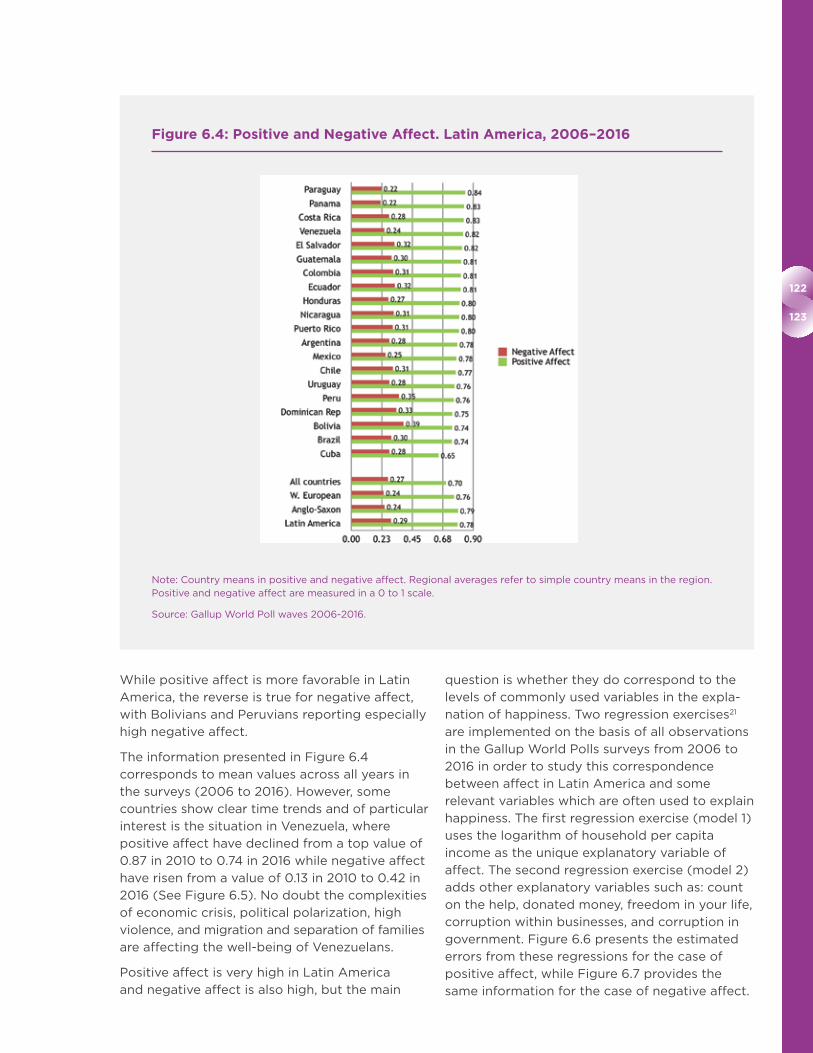
122
123
While positive affect is more favorable in Latin
America, the reverse is true for negative affect,
with Bolivians and Peruvians reporting especially
high negative affect.
The information presented in Figure 6.4
corresponds to mean values across all years in
the surveys (2006 to 2016). However, some
countries show clear time trends and of particular
interest is the situation in Venezuela, where
positive affect have declined from a top value of
0.87 in 2010 to 0.74 in 2016 while negative affect
have risen from a value of 0.13 in 2010 to 0.42 in
2016 (See Figure 6.5). No doubt the complexities
of economic crisis, political polarization, high
violence, and migration and separation of families
are affecting the well-being of Venezuelans.
Positive affect is very high in Latin America
and negative affect is also high, but the main
question is whether they do correspond to the
levels of commonly used variables in the expla-
nation of happiness. Two regression exercises21
are implemented on the basis of all observations
in the Gallup World Polls surveys from 2006 to
2016 in order to study this correspondence
between affect in Latin America and some
relevant variables which are often used to explain
happiness. The first regression exercise (model 1)
uses the logarithm of household per capita
income as the unique explanatory variable of
affect. The second regression exercise (model 2)
adds other explanatory variables such as: count
on the help, donated money, freedom in your life,
corruption within businesses, and corruption in
government. Figure 6.6 presents the estimated
errors from these regressions for the case of
positive affect, while Figure 6.7 provides the
same information for the case of negative affect.
Figure 6.4: Positive and Negative Affect. Latin America, 2006–2016
Note: Country means in positive and negative affect. Regional averages refer to simple country means in the region. Positive and negative affect are measured in a 0 to 1 scale.
Source: Gallup World Poll waves 2006-2016.
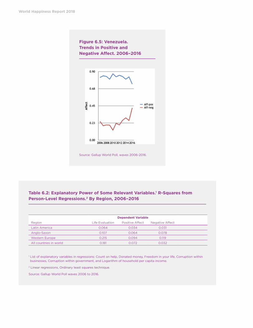
World Happiness Report 2018
Figure 6.5: Venezuela. Trends in Positive and Negative Affect. 2006–2016
Source: Gallup World Poll, waves 2006-2016.
Table 6.2: Explanatory Power of Some Relevant Variables.1 R-Squares from Person-Level Regressions.2 By Region, 2006–2016
Dependent Variable
Region Life Evaluation Positive Affect Negative Affect
Latin America 0.064 0.034 0.031
Anglo-Saxon 0.107 0.064 0.078
Western Europe 0.215 0.094 0.119
All countries in world 0.181 0.072 0.032
1 List of explanatory variables in regressions: Count on help, Donated money, Freedom in your life, Corruption within businesses, Corruption within government, and Logarithm of household per capita income.
2 Linear regressions, Ordinary least squares technique.
Source: Gallup World Poll waves 2006 to 2016.

124
125
It is observed in Figure 6.6 that positive affect is
very high with respect to corresponding income
levels as well as to the situation as described by
a group of variables which are often used to
explain people’s happiness. All Latin American
countries show, on average, positive affect levels
which are much above what would be predicted.
In addition, the regional average in Latin America
is much above that in the Anglo-Saxon and
Western European regions and, of course, much
above the world average (which is 0). Hence, it is
concluded that a strong tendency to experience
above-expected positive emotions is observed in
most Latin American countries. These findings
clearly indicate that the set of explanatory
variables which are commonly used in explaining
happiness is missing some relevant factors which
are relatively abundant in Latin America.
Estimated errors for negative affect in Latin
America do show a pattern which is closer to the
expected one: Some countries show negative
mean errors while others show positive mean
errors, and the regional average is small –but still
significantly different from zero. Hence, it is
concluded that a slight tendency to experience
above-expected negative emotions is observed
in most Latin American countries.
In addition, the explanatory variables of happiness
which are commonly used have less explanatory
power in Latin America. Table 6.2 presents the
goodness of fit (R-square coefficients) for
regional regression exercises with life evaluation,
positive affect, and negative affect as dependent
variables, and with the following variables
as explanatory ones: count on help, donated
Figure 6.6: Positive Affect. Estimated Errors
Notes: Estimated errors from worldwide regression analyses. Positive affect as dependent variable. Independent variables in Model 1: logarithm of household per capita income, count on the help, donated money, freedom in your life, corruption within businesses, and corruption in Government. Independent variables in Model 2: logarithm of household per capita income. Positive affect is measured in a 0 to 1 scale.
Source: Gallup World Poll, all waves 2006 to 2016.

World Happiness Report 2018
money, freedom in your life, corruption within
businesses, corruption within government, and
logarithm of household per capita income. All
observations from the Gallup World Poll surveys
from 2006 to 2016 are used and regressions are
run by region. It is observed in Table 6.2 that
the group of independent variables has good
explanatory power in Western Europe, but very
little explanatory power in Latin America. For
example, while this group of independent
variables explains about 22 percent of the
variability of Western European’s life evaluation
they do only explain about 6 percent of the
variability of Latin Americans’ life evaluation.
Similarly, while the group of variables explains
9 percent of the variability of Western European’s
positive affect – and 12 percent of their negative
affect –, they do only explain 3 percent of the
variability of Latin American’s positive affect –
and 3 percent of their negative affect.
It is evident that Latin Americans are outliers
in what respect to their experience of positive
affect. Latin Americans’ positive affect is high in
comparison to most countries in the world and
also high with respect to what some commonly
Figure 6.7: Negative Affect. Estimated Errors
Notes: Estimated errors from worldwide regression analyses. Negative affect as dependent variable. Independent variables in Model 1: logarithm of household per capita income, count on the help, donated money, freedom in your life, corruption within businesses, and corruption in Government. Independent variables in Model 2: logarithm of household per capita income. Negative affect is measured in a 0 to 1 scale.
Source: Gallup World Poll, all waves 2006 to 2016.

126
127
used explanatory variables would predict. A
slightly similar result is found for negative affect.
Hence, the explanation of happiness on the basis
of variables such as Income, count on help,
donated money, freedom in your life, corruption
within businesses, and corruption within govern-
ment, seems to be missing some very important
drivers, at least for the Latin American case.
Furthermore, the correlation between evaluative
and affective states is smaller in Latin America
than in other regions in the world. Figure 6.8
shows the simple country means by region for
the intra-country correlations22 between affects
(positive and negative) and life evaluation. It is
observed that the regional mean for the intra-
country correlations between positive affect and
life evaluation is much smaller in Latin America
(0.19) than in a group of Anglo-Saxon countries23
(0.32) as well as than in a group of western
European countries (0.28). In a similar way, the
regional mean for the intra-country correlations
between negative affect and life evaluation is
much smaller – in absolute terms – in Latin
America (-0.19) than in a group of Anglo-Saxon
countries (-.34) as well as than in a group of
western European countries (-.28).24
It is also important to state that the regional
mean values for intra-country correlations
between positive and negative affect are very
similar across the regions under study. The
regional mean values are -0.37 in Latin America,
-0.37 in Western Europe, and -0.42 in Anglo-
Saxon countries. In other words, the pattern of
personal correlations between positive and
negative affects does not seem to vary
substantially across regions in the world.
However, the pattern of personal correlations
between positive affect and life evaluation as
well as between negative affect and life
evaluation does substantially differ across
regions.
Figure 6.8: Life Evaluations and Affective States. Intra-Country Correlations, Means by Region
Note: Simple means of intra-country correlations between positive affect (Pos Aff), negative affect (Neg Aff), and life evaluation (LE). Simple means by region.
Source: Gallup World Poll wave 2006 to 2016.
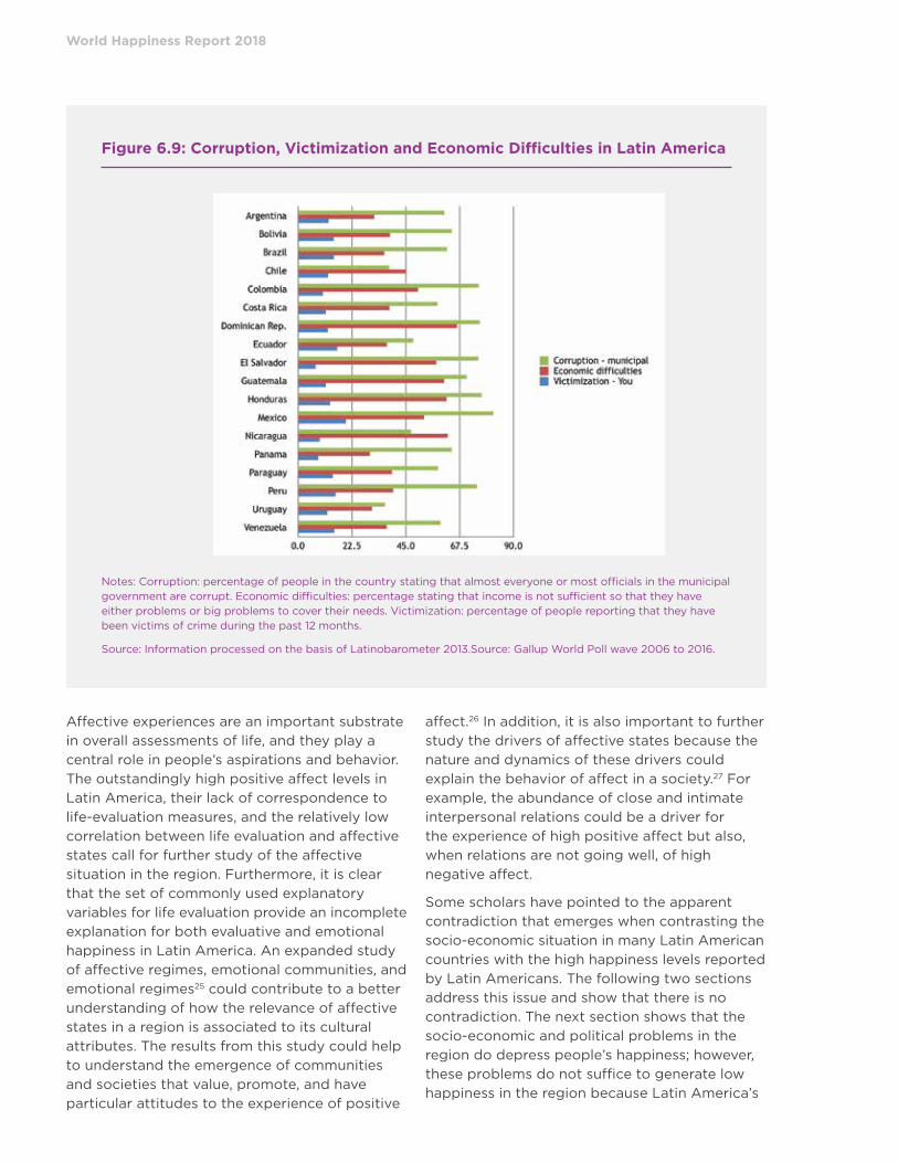
World Happiness Report 2018
Affective experiences are an important substrate
in overall assessments of life, and they play a
central role in people’s aspirations and behavior.
The outstandingly high positive affect levels in
Latin America, their lack of correspondence to
life-evaluation measures, and the relatively low
correlation between life evaluation and affective
states call for further study of the affective
situation in the region. Furthermore, it is clear
that the set of commonly used explanatory
variables for life evaluation provide an incomplete
explanation for both evaluative and emotional
happiness in Latin America. An expanded study
of affective regimes, emotional communities, and
emotional regimes25 could contribute to a better
understanding of how the relevance of affective
states in a region is associated to its cultural
attributes. The results from this study could help
to understand the emergence of communities
and societies that value, promote, and have
particular attitudes to the experience of positive
affect.26 In addition, it is also important to further
study the drivers of affective states because the
nature and dynamics of these drivers could
explain the behavior of affect in a society.27 For
example, the abundance of close and intimate
interpersonal relations could be a driver for
the experience of high positive affect but also,
when relations are not going well, of high
negative affect.
Some scholars have pointed to the apparent
contradiction that emerges when contrasting the
socio-economic situation in many Latin American
countries with the high happiness levels reported
by Latin Americans. The following two sections
address this issue and show that there is no
contradiction. The next section shows that the
socio-economic and political problems in the
region do depress people’s happiness; however,
these problems do not suffice to generate low
happiness in the region because Latin America’s
Figure 6.9: Corruption, Victimization and Economic Difficulties in Latin America
Notes: Corruption: percentage of people in the country stating that almost everyone or most officials in the municipal government are corrupt. Economic difficulties: percentage stating that income is not sufficient so that they have either problems or big problems to cover their needs. Victimization: percentage of people reporting that they have been victims of crime during the past 12 months.
Source: Information processed on the basis of Latinobarometer 2013.Source: Gallup World Poll wave 2006 to 2016.

128
129
social organization promotes and nurtures some
drivers of happiness which are not fully captured
by commonly-used explanatory variables. The
following section elaborates an explanation of
Latin Americans’ happiness in terms of the
importance human relations have in the region,
not only as a source of material support but,
fundamentally, as a source of positive affect and
of non-materialistic purpose in life. In particular,
the abundance and the quality of family relations
play a crucial role in understanding happiness in
Latin America.
Social, Economic and Political Problems in Latin America and Their Impact on Happiness
Latin America is no paradise; there are many
social and economic problems in the region.
Some of the problems are structural and emerge
from historical processes, such as: weak political
institutions, high corruption levels, and high
income inequality that magnifies poverty rates in
what would mostly be considered as mid-income
countries. Other problems have been triggered
by recent processes; for example: the closeness
to the largest drug market in the world combined
with a wrong strategy that looks to represses
production rather than to reduce consumption
has exacerbated drug-related violence and has
led to alarming crime rates in some areas of Latin
America. This process of rising violence is also
fostered by weak civic interpersonal relations,
high corruption rates, and greater penetration
of materialistic values during the last decades.
Figure 6.9 shows some figures on corruption,
victimization and economic difficulties which
suffice to portray the situation of social problems
in the region. The belief that there is some level
of corruption at the local and national govern-
mental levels is widespread in Latin America.
Country level figures for municipal-level
corruption go as high as 82 percent in Mexico;
with relatively low figures -beneath 40 percent-
in Chile and Uruguay.28
Living within some degree of economic difficulty
is also common in most countries of Latin
America. For example, about 36 percent of
Brazilians and 53 percent of Mexicans declare
Table 6.3: Corruption, Economic Difficulties and Victimization. Impact on Life Satisfaction
Coefficient Prob>t
Perception of corruption municipal level
Almost everyone is corrupt -0.106 0.000
Most officials are corrupt -0.093 0.000
Not many officials are involved -0.050 0.045
There is hardly anyone involved Reference
Economic difficulties. Problems or big problems to cover their needs
It is not sufficient, has big problems -0.409 0.000
It is not sufficient, has problems -0.242 0.000
It is just sufficient, does not have major problems -0.036 0.066
It is sufficient, can save Reference
Victimization during the past 12 months
both you and relative -0.126 0.000
you -0.067 0.000
relative -0.042 0.003
none Reference
R2 0.116
Note. Control variables: marital state, gender, age, age squared, education level, language, country dummies.
Source: Latinobarometer 2013.
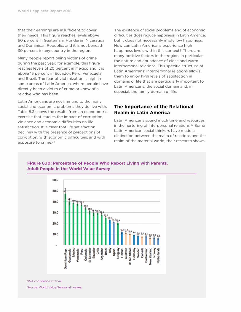
World Happiness Report 2018
that their earnings are insufficient to cover
their needs. This figure reaches levels above
60 percent in Guatemala, Honduras, Nicaragua
and Dominican Republic, and it is not beneath
30 percent in any country in the region.
Many people report being victims of crime
during the past year; for example, this figure
reaches levels of 20 percent in Mexico and it is
above 15 percent in Ecuador, Peru, Venezuela
and Brazil. The fear of victimization is high in
some areas of Latin America, where people have
directly been a victim of crime or know of a
relative who has been.
Latin Americans are not immune to the many
social and economic problems they do live with.
Table 6.3 shows the results from an econometric
exercise that studies the impact of corruption,
violence and economic difficulties on life
satisfaction. It is clear that life satisfaction
declines with the presence of perceptions of
corruption, with economic difficulties, and with
exposure to crime.29
The existence of social problems and of economic
difficulties does reduce happiness in Latin America,
but it does not necessarily imply low happiness.
How can Latin Americans experience high
happiness levels within this context? There are
many positive factors in the region, in particular
the nature and abundance of close and warm
interpersonal relations. This specific structure of
Latin Americans’ interpersonal relations allows
them to enjoy high levels of satisfaction in
domains of life that are particularly important to
Latin Americans: the social domain and, in
especial, the family domain of life.
The Importance of the Relational Realm in Latin America
Latin Americans spend much time and resources
in the nurturing of interpersonal relations.30 Some
Latin American social thinkers have made a
distinction between the realm of relations and the
realm of the material world; their research shows
Figure 6.10: Percentage of People Who Report Living with Parents. Adult People in the World Value Survey
95% confidence interval
Source: World Value Survey, all waves.
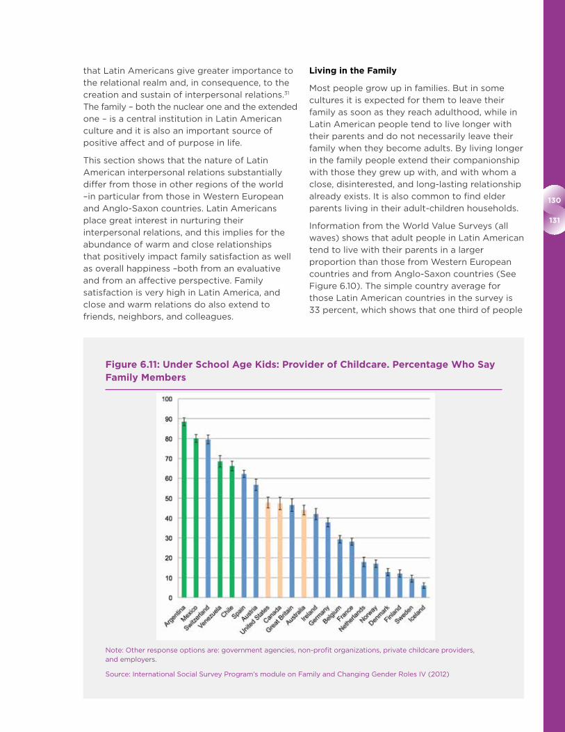
130
131
that Latin Americans give greater importance to
the relational realm and, in consequence, to the
creation and sustain of interpersonal relations.31
The family – both the nuclear one and the extended
one – is a central institution in Latin American
culture and it is also an important source of
positive affect and of purpose in life.
This section shows that the nature of Latin
American interpersonal relations substantially
differ from those in other regions of the world
–in particular from those in Western European
and Anglo-Saxon countries. Latin Americans
place great interest in nurturing their
interpersonal relations, and this implies for the
abundance of warm and close relationships
that positively impact family satisfaction as well
as overall happiness –both from an evaluative
and from an affective perspective. Family
satisfaction is very high in Latin America, and
close and warm relations do also extend to
friends, neighbors, and colleagues.
Living in the Family
Most people grow up in families. But in some
cultures it is expected for them to leave their
family as soon as they reach adulthood, while in
Latin American people tend to live longer with
their parents and do not necessarily leave their
family when they become adults. By living longer
in the family people extend their companionship
with those they grew up with, and with whom a
close, disinterested, and long-lasting relationship
already exists. It is also common to find elder
parents living in their adult-children households.
Information from the World Value Surveys (all
waves) shows that adult people in Latin American
tend to live with their parents in a larger
proportion than those from Western European
countries and from Anglo-Saxon countries (See
Figure 6.10). The simple country average for
those Latin American countries in the survey is
33 percent, which shows that one third of people
Figure 6.11: Under School Age Kids: Provider of Childcare. Percentage Who Say Family Members
Note: Other response options are: government agencies, non-profit organizations, private childcare providers, and employers.
Source: International Social Survey Program’s module on Family and Changing Gender Roles IV (2012)

World Happiness Report 2018
Figure 6.12: Provider of Domestic Help to Elderly People. Percentage Who Say it is for Family Members to Take Care of Domestic Help for Elderly People
Note: Other response options are: government agencies, non-profit organizations, private childcare providers, and employers.
Source: International Social Survey Program’s module on Family and Changing Gender Roles IV (2012)
Figure 6.13: Taking Care of Family Before Helping Others. Country Means
Note: You should take care of yourself and your family first, before helping other people. Response scale: 5 Agree strongly, 4 agree, 3 neither agree nor disagree, 2 disagree, 1 disagree strongly.
Source: International Social Survey Program, Social Networks II, 2001.

132
133
who were surveyed reported living with their
parents. This figure is only 12 percent for those
western European countries and only 9 percent
for those Anglo-Saxon countries included in
Figure 6.10.
The extension of children’s stay at home as well
as the incorporation of the elders in their grown-
up children’s households implies an abundance
of close and normally supportive interpersonal
relationships. When these relationships are
gratifying they do contribute to both high live
evaluation and the enjoyment of high positive
affect; however, in those cases where the
intimate relationships become unsatisfactory
they may detonate the experience of strong
negative affect.32
Taking Care of Children and Elderly in the Family
Family members do also play a central role in
child rearing in Latin America, and many elder
persons do live with their adult children and their
grandchildren and/or do keep in close contact
with them.
The International Social Survey Program’s
module on Family and Changing Gender Roles IV
(2012) asked the following two questions to
people from many countries: First, ‘People have different views on childcare for children under school age. Who do you think should primarily provide childcare?’, second, ‘Thinking about elderly people who need some help in their everyday lives, such as help with grocery shopping, cleaning the house, doing the laundry etc. Who do you think should primarily provide this help?’. The information from the survey
shows that Latin Americans strongly believe that
the family must play a central role in raising kids
as well as in taking care of the elder. The simple
Figure 6.14: One of Main Goals: Make My Parents Proud. Country Means
Note: Making parents proud as one of the main goals in life. Response scale: Strongly agree (4), Agree (3), Disagree (2), Strongly disagree (1)
Source: World Value Survey, all waves.

World Happiness Report 2018
country average for people responding that the
family should take care of under-school age kids
is 76 percent in the Latin American countries in
the survey. The same figure is only 33 percent
for Western European countries and 46 percent
for Anglo-Saxon countries in the survey (See
Figure 6.11).
Similarly, a larger proportion of Latin Americans
do also believe that elderly people should be
supported by their family members rather than
by governmental and private institutions. The
simple country average for those Latin American
countries in the survey is 77 percent, while this
figure is 36 percent in the Western European
countries and 52 percent in the Anglo Saxon
countries in Figure 6.12.
A larger proportion of under-school-age
children in Latin America grow up within a
family environment and enjoying the close
interaction with people who love them and
who are intrinsically motivated to take care of
them. Elder people do also frequently enjoy the
company of loved ones. Research has shown that
there are positive emotional benefits of growing
in family environments where parents are present
in the raising of their kids.33
Preference for Taking Care of Family
The ISSP Social Networks II survey (2001) asked
people about their degree of agreement with the
following statement: “You should take care of yourself and your family first, before helping other people”. There were only two Latin American
countries in this survey, but the data shows that
people in Brazil – Latin America’s largest country
– tend to strongly agree with this statement,
while in Chile people do agree with the statement
(Figure 6.13).
Figure 6.15: Watching Children Grow is Greatest Joy. Country Means
Note: Watching children grow up is greatest joy. Response scale: 5 Strongly agree, 4 Agree, 3 Neither agree nor disagree, 2 Disagree, 1 Strongly disagree.
Source: International Social Survey Program’s module on Family and Changing Gender Roles IV (2012)
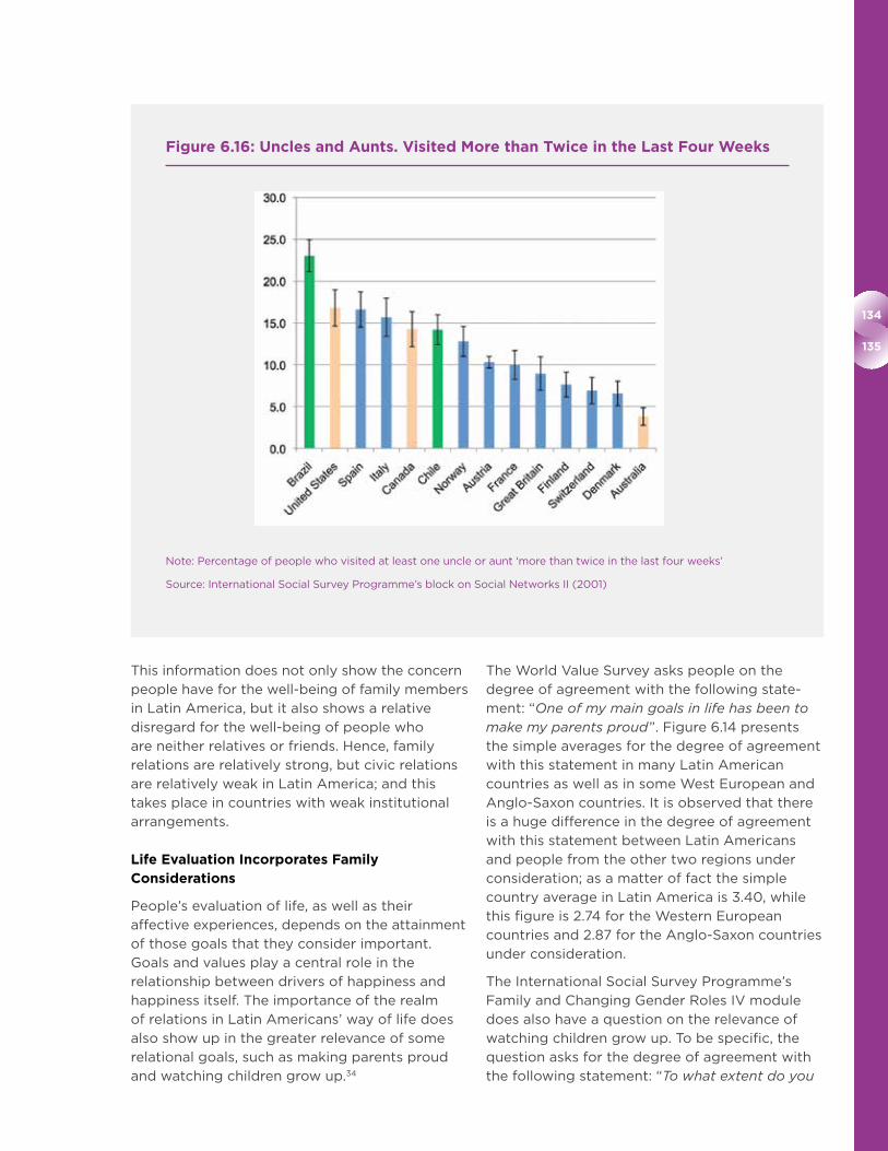
134
135
This information does not only show the concern
people have for the well-being of family members
in Latin America, but it also shows a relative
disregard for the well-being of people who
are neither relatives or friends. Hence, family
relations are relatively strong, but civic relations
are relatively weak in Latin America; and this
takes place in countries with weak institutional
arrangements.
Life Evaluation Incorporates Family Considerations
People’s evaluation of life, as well as their
affective experiences, depends on the attainment
of those goals that they consider important.
Goals and values play a central role in the
relationship between drivers of happiness and
happiness itself. The importance of the realm
of relations in Latin Americans’ way of life does
also show up in the greater relevance of some
relational goals, such as making parents proud
and watching children grow up.34
The World Value Survey asks people on the
degree of agreement with the following state-
ment: “One of my main goals in life has been to make my parents proud”. Figure 6.14 presents
the simple averages for the degree of agreement
with this statement in many Latin American
countries as well as in some West European and
Anglo-Saxon countries. It is observed that there
is a huge difference in the degree of agreement
with this statement between Latin Americans
and people from the other two regions under
consideration; as a matter of fact the simple
country average in Latin America is 3.40, while
this figure is 2.74 for the Western European
countries and 2.87 for the Anglo-Saxon countries
under consideration.
The International Social Survey Programme’s
Family and Changing Gender Roles IV module
does also have a question on the relevance of
watching children grow up. To be specific, the
question asks for the degree of agreement with
the following statement: “To what extent do you
Figure 6.16: Uncles and Aunts. Visited More than Twice in the Last Four Weeks
Note: Percentage of people who visited at least one uncle or aunt ‘more than twice in the last four weeks’
Source: International Social Survey Programme’s block on Social Networks II (2001)
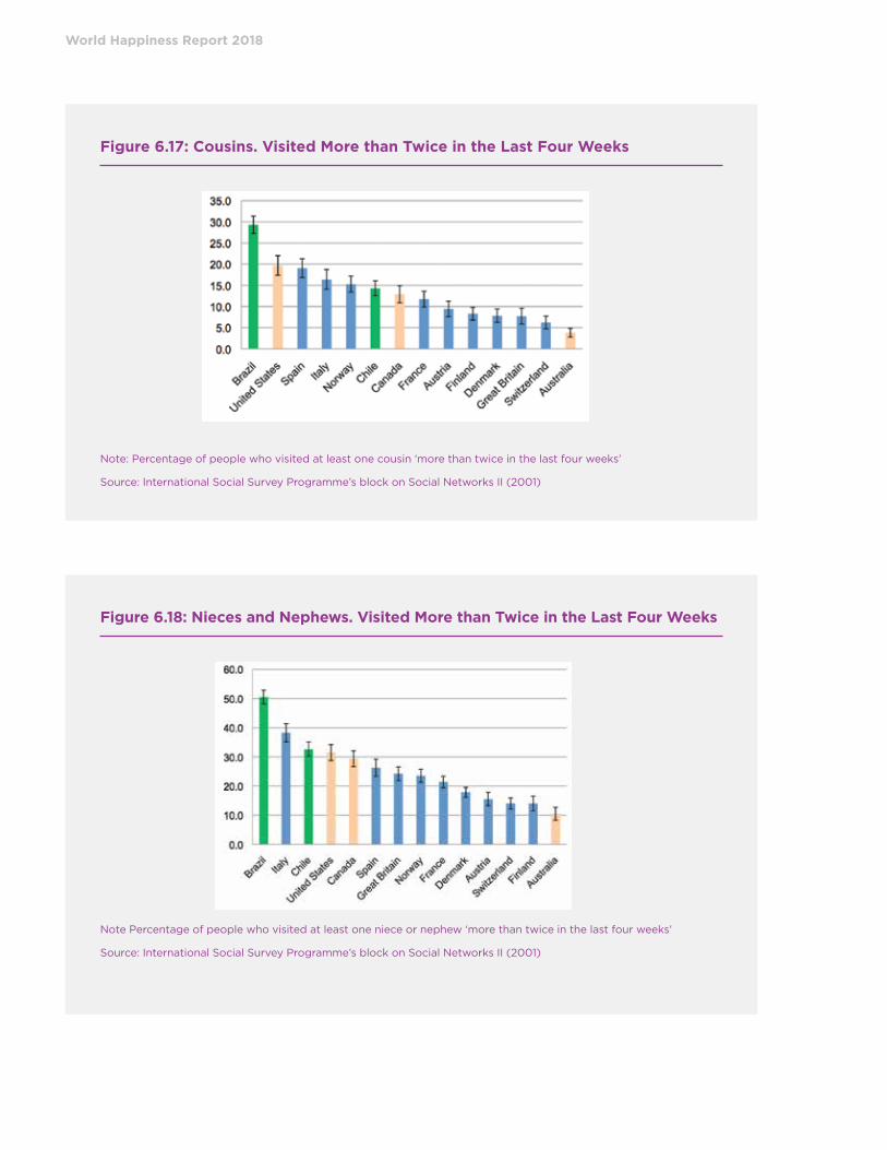
World Happiness Report 2018
Figure 6.17: Cousins. Visited More than Twice in the Last Four Weeks
Note: Percentage of people who visited at least one cousin ‘more than twice in the last four weeks’
Source: International Social Survey Programme’s block on Social Networks II (2001)
Figure 6.18: Nieces and Nephews. Visited More than Twice in the Last Four Weeks
Note Percentage of people who visited at least one niece or nephew ‘more than twice in the last four weeks’
Source: International Social Survey Programme’s block on Social Networks II (2001)
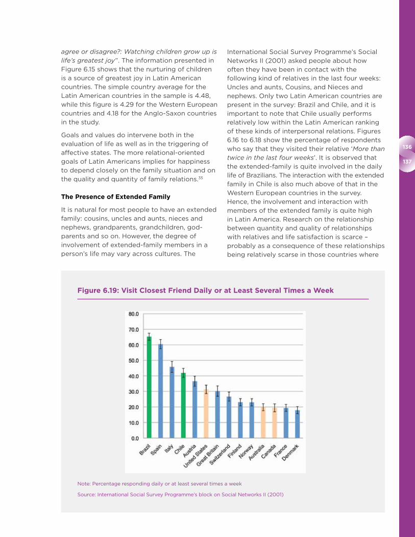
136
137
agree or disagree?: Watching children grow up is life’s greatest joy”. The information presented in
Figure 6.15 shows that the nurturing of children
is a source of greatest joy in Latin American
countries. The simple country average for the
Latin American countries in the sample is 4.48,
while this figure is 4.29 for the Western European
countries and 4.18 for the Anglo-Saxon countries
in the study.
Goals and values do intervene both in the
evaluation of life as well as in the triggering of
affective states. The more relational-oriented
goals of Latin Americans implies for happiness
to depend closely on the family situation and on
the quality and quantity of family relations.35
The Presence of Extended Family
It is natural for most people to have an extended
family: cousins, uncles and aunts, nieces and
nephews, grandparents, grandchildren, god-
parents and so on. However, the degree of
involvement of extended-family members in a
person’s life may vary across cultures. The
International Social Survey Programme’s Social
Networks II (2001) asked people about how
often they have been in contact with the
following kind of relatives in the last four weeks:
Uncles and aunts, Cousins, and Nieces and
nephews. Only two Latin American countries are
present in the survey: Brazil and Chile, and it is
important to note that Chile usually performs
relatively low within the Latin American ranking
of these kinds of interpersonal relations. Figures
6.16 to 6.18 show the percentage of respondents
who say that they visited their relative ‘More than twice in the last four weeks’. It is observed that
the extended-family is quite involved in the daily
life of Brazilians. The interaction with the extended
family in Chile is also much above of that in the
Western European countries in the survey.
Hence, the involvement and interaction with
members of the extended family is quite high
in Latin America. Research on the relationship
between quantity and quality of relationships
with relatives and life satisfaction is scarce –
probably as a consequence of these relationships
being relatively scarse in those countries where
Figure 6.19: Visit Closest Friend Daily or at Least Several Times a Week
Note: Percentage responding daily or at least several times a week
Source: International Social Survey Programme’s block on Social Networks II (2001)

World Happiness Report 2018
major research is undertaken –; however, some
findings suggest that this kind of relationship
may contribute to people’s happiness.36
Close Relationships with Close Friends
The realm of close interpersonal relations in Latin
America extends beyond the nuclear and extended
family. Friends are also highly involved in the
daily life of Latin Americans, and friends are
expected to play an important role not only in
bringing emotional and economic support but
also in sharing daily life.
The International Social Survey Programme’s
block on Social Networks II (2001) has a couple of
questions regarding the involvement and support
which is expected from friends in different coun-
tries of the world. Two Latin American countries
are included in this survey: Brazil and Chile.
The first question asks how often people see
or visit their closest friend. Figure 6.19 shows
the percentage of people who report seeing or
visiting their closest friend daily or at least
several times a week. It is observed that this
percentage is very high in Brazil and it is also
high in Chile.
The second question asks people about their
degree of agreement with the following statement:
“People who are better off should help friends who are less well off”. Figure 6.20 shows that in the two
Latin American countries in the survey there is
wide agreement about expecting friends who are
better off to help those who are less well off.
Data from other sources, such as the BIARE-
Mexico (National Statistical Office survey on
self-reported well-being) and the United States’
General Social Survey show that people in
Mexico gather more often and more frequently
with relatives and with friends than people in the
United States. For example, 77 percent of people
in Mexico state that they gather with relatives at
least several times per month, while this figure is
of 53 percent in the United States. Regarding
gathering with friends several times per month,
the figure is 68 percent in Mexico and 45 percent
in the United States.
Figure 6.20: People Better Off Should Help Friends
Note: Country averages; people who are better off should help their friends. Response scale: 5 Agree strongly, 4 agree, 3 neither agree nor disagree, 2 disagree, 1 disagree strongly
Source: International Social Survey Programme’s block on Social Networks II (2001)
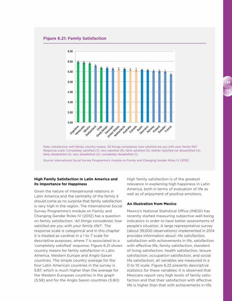
138
139
High Family Satisfaction in Latin America and its Importance for Happiness
Given the nature of interpersonal relations in
Latin America and the centrality of the family it
should come as no surprise that family satisfaction
is very high in the region. The International Social
Survey Programme’s module on Family and
Changing Gender Roles IV (2012) has a question
on family satisfaction: ‘All things considered, how satisfied are you with your family life?’. The
response scale is categorical and in this chapter
it is treated as cardinal in a 1 to 7 scale for
descriptive purposes, where 7 is associated to a
‘completely satisfied’ response. Figure 6.21 shows
country means for family satisfaction in Latin
America, Western Europe and Anglo-Saxon
countries. The simple country average for the
four Latin American countries in the survey is
5.87, which is much higher than the average for
the Western European countries in the graph
(5.58) and for the Anglo Saxon countries (5.60)
High family satisfaction is of the greatest
relevance in explaining high happiness in Latin
America, both in terms of evaluation of life as
well as of enjoyment of positive emotions.
An Illustration from Mexico
Mexico’s National Statistical Office (INEGI) has
recently started measuring subjective well-being
indicators in order to have better assessments of
people’s situation. A large representative survey
(about 39,000 observations) implemented in 2014
provides information about: life satisfaction,
satisfaction with achievements in life, satisfaction
with affective life, family satisfaction, standard
of living satisfaction, health satisfaction, leisure
satisfaction, occupation satisfaction, and social
life satisfaction. all variables are measured in a
0 to 10 scale. Figure 6.22 presents descriptive
statistics for these variables; it is observed that
Mexicans report very high levels of family satis-
faction and that their satisfaction with affective
life is higher than that with achievements in life.
Figure 6.21: Family Satisfaction
Note: Satisfaction with family, country means. ‘All things considered, how satisfied are you with your family life?’ Response scale: Completely satisfied (7), very satisfied (6), fairly satisfied (5), neither satisfied nor dissatisfied (4), fairly dissatisfied (3), very dissatisfied (2), completely dissatisfied (1).
Source: International Social Survey Programme’s module on Family and Changing Gender Roles IV (2012)
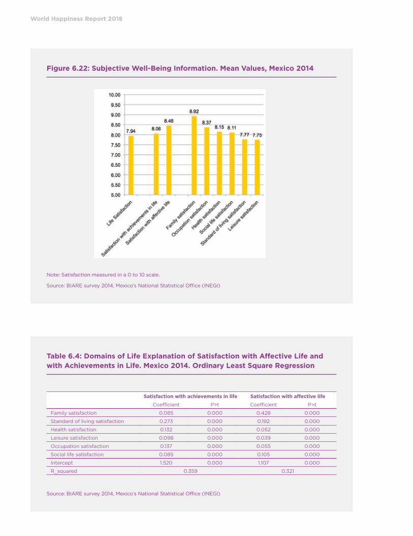
World Happiness Report 2018
Figure 6.22: Subjective Well-Being Information. Mean Values, Mexico 2014
Note: Satisfaction measured in a 0 to 10 scale.
Source: BIARE survey 2014, Mexico’s National Statistical Office (INEGI)
Table 6.4: Domains of Life Explanation of Satisfaction with Affective Life and with Achievements in Life. Mexico 2014. Ordinary Least Square Regression
Satisfaction with achievements in life Satisfaction with affective life
Coefficient P>t Coefficient P>t
Family satisfaction 0.085 0.000 0.428 0.000
Standard of living satisfaction 0.273 0.000 0.192 0.000
Health satisfaction 0.132 0.000 0.052 0.000
Leisure satisfaction 0.098 0.000 0.039 0.000
Occupation satisfaction 0.137 0.000 0.055 0.000
Social life satisfaction 0.085 0.000 0.105 0.000
Intercept 1.520 0.000 1.107 0.000
R_squared 0.359 0.321
Source: BIARE survey 2014, Mexico’s National Statistical Office (INEGI)
140
141
Relatively low levels of satisfaction are seen in
the standard of living and leisure (free-time)
domains of life.
Table 6.4 presents the main results from an
econometric exercise that aims at explaining
satisfaction with achievements in life and with
affective life on the basis of satisfaction in
domains of life.
It is observed that family satisfaction has, by
far, the largest impact on the satisfaction with
affective life of Mexicans. Family satisfaction
is also statistically significant in explaining
satisfaction with achievements in life; however,
in this case the standard of living has a much
larger coefficient. It seems that interpersonal
relations matter for both affective and evaluative
aspects of life, but they count more for the
former than for the latter.37
Conclusions
Latin Americans report high happiness levels.
Positive-affect scores are substantially high both
in comparison to other countries in the world
and to what income levels in the region would
predict. Latin Americans’ evaluation of life is also
above what income levels would predict.
Many social and economic indicators portray
Latin America as a mid to low income-level
region with high poverty rates, great income
inequality, high violence and crime rates, and high
levels of corruption. How can Latin Americans
be so happy within a context that may look
somehow unfavorable? This chapter has shown
that the happiness of Latin Americans is
diminished by their many social and economic
problems and that, in fact, happiness could
increase if these problems were properly
addressed. However, it would be a big mistake to
assume that these problems overwhelm the daily
lives of Latin Americans. In fact, it would be a
focusing-illusion bias to assume that Latin
Americans must be unhappy because there are
some problems in their life. In fact, the daily life
of Latin Americans is not constricted to the
consequences of income poverty, institutional
corruption, income inequality, crime and
violence, and other problems. This chapter
shows that there are many positive factors that
contribute to the happiness of Latin Americans;
in particular, the abundance and quality of close,
warm, and genuine interpersonal relations.
The specific structure of Latin Americans’
interpersonal relations allows them to enjoy high
levels of satisfaction in domains of life that are
particularly important to Latin Americans: the
social domain and, in especial, the family domain
of life. It explains the outstandingly high positive
affect in the region as well as the above-expected
evaluative states.
The Latin American case shows that the
abundance and nature of interpersonal relations
is an important driver of happiness which
deserves further attention, as was emphasized
in Chapter 2 of World Happiness Report 2017.
Happiness research that focuses on evaluative
measures may risk underestimating the impor-
tance that close, warm and genuine interpersonal
relations have in people’s happiness because
their impact is larger on affective than on
evaluative states. Happiness in relational-
oriented societies may be better portrayed by
overall assessments of life that incorporate
information from both the evaluative and the
affective substrates.
There are many lessons from the Latin American
case to the development discourse.
First, it shows the need of going beyond
objective measures when aiming to assess
people’s situation. Subjective well-being
measures provide better assessments of the
experience of being well people have and
contribute to a better understanding of their
actions. Subjective well-being measures better
incorporate the values people have and which
are relevant in assessing their lives; because
values differ across cultures this subjectivity
constitutes an advantage when making
cross-cultural assessments of people’s
well-being.
Second, the Latin American case does not ignore
the importance of income, but it clearly shows
that there is more to life than income. The
development discourse should neither confuse
persons with consumers nor well-being with
purchasing power.
Third, the Latin American case shows that
genuine, warm, and person-based interpersonal
relations substantially contribute to happiness.
The development discourse has neglected these
relations in favor of instrumental ones, which
World Happiness Report 2018
may have a larger impact on economic growth
but not on people’s happiness. By objectifying
other people, instrumental relations are not as
gratifying as genuine ones.
Fourth, it is not only acceptable for but also
expected from public policy to focus on solving
social problems; however, such policies will not
succeed in raising happiness if they neglect the
positive aspects of social life, and if they follow a
partial rather than integral view. In fact, policies
should not focus only on eradicating problems
but also on strengthening those riches Latin
Americans currently have.
142
143
Endnotes
1 According to the Human Development Report 2017 Mexico, Costa Rica, Panamá, Cuba, Dominican Republic, Colombia, Venezuela, Ecuador, Peru, Brazil and Uruguay are classified as ‘High Human Development’. Chile and Argentina are classified as ‘Very High Human Development’. Guatemala, El Salvador, Honduras, Nicaragua, Bolivia and Paraguay are classified as ‘Medium Development’. Haiti, which has a different history, is the only country in the region classified as ‘Low Human Development’.
2 Rojas (2012a), Beytía (2016, 2018), Yamamoto (2016)
3 Rojas & García (2017)
4 Puchet et al. (2012), Rojas (2012b), Casas-Zamora and Carter (2017), O’Donnell (1999), Gasparini and Lustig (2011), Jaitman (2017), World Bank (2011)
5 Culture is neither static nor fully determined by past events and the concept involves extreme simplification and homogenization (Holler, 2014); however, it is relevant to explain the phenomenon of high happiness in Latin America.
6 It is important to recognize that the Mayan civilization had seen better times in the past.
7 Bushnell et al. (2017) mention the following factors promoting the mixing of Europeans and Indians in Latin America: The relatively scarcity of Spanish women in the new territory induced male Spaniards to quickly mixed with indigenous women. Inter-ethnic mixing was no alien to Spanish conquerors and colonizers as a result of the recent history of coexistence of Moors and Christians in the Iberian Peninsula. The idea of accumulating wealth before marrying was common among Spanish men, and the custom of having illegitimate children was already widely spread in Spain at the time of conquest and colony. In addition, the indigenous civilizations had social hierarchies, with many male and female Indians enjoying high social status.
8 Las Casas (1945, 1951, 1967), Díaz del Castillo (1955), León-Portilla (2014), Estrada (2009)
9 Bonfill (1994), Morandé (1971, 1985), Zea (1971, 1985), Larraín (1971), de Imaz (1984). It is important to remark that the blending of values and worldviews does not necessarily imply the complete integration of Europeans and indigenous groups; many studies show that even today there is some discrimination on the basis of the skin color (Ortiz et al., 2018)
10 Noguera and Pineda (2011), Ángel Maya (1995, 2002, 2006)
11 Acosta (2008), Gudynas and Acosta (2011)
12 Esteinou (2004), Arizpe (1973), Gonzalbo (1996, 1998), Gonzalbo and Rabell (1996)
13 Díaz-Guerrero (1979), Germany (1965), Díaz-Loving et al. (2008).
14 Rojas & García-Vega (2017), Yamamoto (2016), Beytía (fc), Velásquez (2016), Martínez Cruz & Castillo Flores (2016), Mochón Morcillo & de Juan Díaz (2016), Ateca-Amestoy et al. (2014).
15 The specific countries which are included in the Western European and Anglo-Saxon lists may vary across analyses due to the availability of information. However, in general the Western European classification makes reference to the following countries: United Kingdom, France, Germany, Netherlands, Belgium, Spain, Italy, Sweden, Greece, Denmark, Austria, Cyprus, Finland, Iceland, Luxembourg,
Switzerland, Norway, Portugal, and Ireland. The Anglo- Saxon classification makes reference to the following countries: United States, Canada, Australia, and New Zealand.
16 Life evaluation is measured on the following question from the Gallup Polls: “Please imagine a ladder with steps numbered from zero at the bottom to ten at the top. Suppose we say that the top of the ladder represents the best possible life for you, and the bottom of the ladder represents the worst possible life for you. On which step of the ladder would you say you personally feel you stand at this time, assuming that the higher the step the better you feel about your life, and the lower the step the worse you feel about it? Which step comes closest to the way you feel?” The response to the question is based on an imaginary 11-point scale whereby 0 designates one’s worst possible life and 10 denotes the best possible life respondents can imagine for themselves.
17 Figures are computed using information from the Gallup World Poll waves 2006 to 2016. The survey includes 166 countries and regions.
18 If you were in trouble, do you have relatives or friends you can count on to help you whenever you need them, or not? (1=yes, 0=no). Donated money to a charity (1=yes, 0=no). Whether the respondent is satisfied with the freedom to choose what do to with his or her life in this country (1=yes, 0=no). Whether the respondent thinks there is corruption in businesses (1=yes, 0=no). Whether the respondent thinks there is corruption in government (1=yes, 0=no).
19 The five dichotomous variables are: Smile or laugh yesterday, learn something, treated with respect, experienced enjoyment, and feel well-rested. The questions in the survey ask whether this affect was experienced the day before.
20 Negative affect is assessed as the simple average of the following dichotomous variables in the Gallup World Poll: Experience worry, Sadness, Anger, Stress, and Depression. The Gallup survey asks whether the person experienced the emotion the day before, with a Yes or No answer.
21 The regression exercises use an ordinary least square technique, which means that the independent variable is treated as a cardinal one.
22 By intra-country correlations we mean the correlations between affect and life evaluation based on differences across persons living in the same country.
23 Canada, United States, Australia and New Zealand.
24 It is also possible to estimate regional correlations based on country mean values of life evaluation, and positive and negative affect. It is found that these correlations do also differ across regions. For example, the correlation between country means of positive affect and life evaluation is 0.87 in the Western European region and only 0.29 in the Latin American region. Similarly, the correlation between negative affect and life evaluation is -0.90 in the western European region and only -.36 in the Latin American region. This finding basically indicates that by knowing a Western European country’s life evaluation mean it is possible to predict with high confidence this country’s positive and negative-affect means; however, this would not be possible for Latin American countries, where a relatively high life evaluation is not necessarily associated to a relatively high positive affect or a relatively low negative affect in a country.
25 Sterns and Sterns, 1985; Rosenweim, 2002; Reddy, 2001.
26 Holler, 2014; Villa-Flores and Lipsett-Rivera, 2014; Rivera, 2000. It may also be interesting to note that a study of human language found that Latin American languages show the greatest positivity in comparison to other languages in the study. The authors state that “Mexican Spanish and Brazilian Portuguese exhibit relatively high medians” (Dodds et al., 2015; p. 2390) in perceived average word happiness for 10 languages under study.
27 Rojas, 2013; Rojas and Guardiola, 2017.
28 Some international data shows that corruption in Latin America is comparatively high. Transparency International’s Corruption Perception Index (CPI) goes from 0 (highest level of perceived corruption) to 100 (lowest level of perceived corruption). The mean value of the CPI for Latin American countries is 37.9, which is slightly lower than the mean value for the world (42.9) and much lower than the value for Western European countries (74.8) and for the Anglo-Saxon countries (81.2). This means that Latin America’s perceived corruption level is higher than the world average and much higher than those levels in Western Europe and the Anglo-Saxon countries, according to data from 2016 of Transparency International. Uruguay, Chile and Costa Rica present the lowest levels of perceived corruption in Latin America, while Guatemala, Nicaragua and Venezuela present the highest levels.
29 Country-level studies suggest that negative events such as corruption and victimization trigger negative affect and reduce life evaluation (Leyva et al., 2016)
30 In some towns of Mexico people do also spend a lot of time and resources nourishing their relationship with the dead ones. The night before The Day of the Death (November 2nd) the living ones gather in the cemeteries with their dead relatives in order to celebrate and eat together. Relatives are always present, even after they have died.
31 Díaz Guerrero (1997)
32 See Leyva et al., 2016. It may be stated that in terms of the experience of affective states close, warm, and disinterest-ed interpersonal relations provide greater mean returns but also greater risk.
33 For the importance of parent-child relationships see Noble and McGrath (2012) and O’Brien and Mosco (2012) For a review of many studies on the emotional benefits of family relationships see Kasser (2002) For an in-depth study of the importance of parent-child relationships for life satisfaction over the life course see Layard et al. (2013) and Clark et al. (2018)
34 Germani (1965); Díaz-Guerrero (1979); Yamamoto (2016)
35 Domains-of-life studies in Latin America show that the family domain is crucial in explaining life satisfaction as well as its evaluative and affective substrates (Rojas, 2006, 2012c)
36 On the basis of information from the United Kingdom Powdthavee (2008) finds that frequency of contact with relatives –as well as with friends- does make a significant impact on people’s happiness. Powdthavee concludes that “the estimated figure is even larger than that of getting married . . . It can compensate for nearly two-third in the loss of the happiness from going through a separation or unemployment”. Nguyen at al. (2016) also find that the frequency of contact with family members has a positive impact on life satisfaction, happiness and self-esteem; however, the delimitation of family members is not clear in
the study. There is also some research finding out that inter-generational family relations are very relevant for the well-being of elder people (Katz, 2009) Of course, there is also an ample literature on relational goods which empha-sizes the importance of interpersonal relations without providing an in-depth study of specific kinds of family relations (Gui, 2005; Gui and Stanca, 2010; Becchetti et al., 2008) Relatedness is also considered a basic psychological need by Deci and Ryan (1985), while Grinde (2009) elaborates an evolutionary argument about the importance of community relations for people’s well-being.
37 Life satisfaction is highly correlated with both satisfaction with affective life (0.42) and satisfaction with achievements in life (0.46).
World Happiness Report 2018

144
145
References
Acosta, A. (2008). El buen vivir, una oportunidad por construir. Ecuador Debate, 75, 33-47.
Ángel Maya, A. (1995). La fragilidad ambiental de la cultura. Bogotá: Editorial Universidad Nacional Instituto de Estudios Ambientales IDEA.
Ángel Maya, A. (2006). Ataraxia. Cali: Universidad Autónoma de Occidente.
Ángel Maya, A. (2002). El retorno de Icaro; Serie La Razón de la Vida X. Pensamiento ambiental latinoamericano 3, Bogotá: ASOCAR, IDEA, PNUMA, PNUD.
Arizpe, L. (1973). Parentezco y economía en una sociedad nahua. México: Colección SEP-INI.
Ateca-Amestoy, V., Cortés Aguilar, A., & Moro-Egido A. (2014). Social interactions and subjective well-being: Evidence from Latin America. Journal of Happiness Studies, 15, 527-554.
Becchetti, L., Pelloni, A., & Rossetti, F. (2008). Relational goods, sociability, and happiness. Kyklos 61(3), 343-363.
Beytía, P. (2018). The efficiency of subjective well-being: A key of Latin American development. In Bula, G., & Masaheli, M. (Eds.). Latin American perspectives on global development. Cambridge: Cambridge Scholars Publishing.
Beytía, P. (2016). The singularity of Latin American patterns of happiness. In Rojas, M. (Ed.) Handbook of happiness research in Latin America, Springer.
Beytía, P. (forthcoming). Vínculos familiares: una clave explicativa de la felicidad. In Reyes, C. & Muñoz, M. La familia en tiempos de cambio. Ediciones UC.
Bonfil, G. (1994). México Profundo. Una civilización negada. México DF: Editorial Grijalbo.
Bushnell, D., Lockhart, J., & Kittleson, R.A. (2017). History of Latin America, Encyclopedia Britannica. Retrieved from www.britannica.com/place/Latin-America.
Casas-Zamora, K., & Carter, M. (2017). Beyond the scandals: The changing context of corruption in Latin America, Washington DC: Inter-American Dialogue.
Clark, A.E., Flèche, S., Layard, R., Powdthavee, N., & Ward, G. (2018) The origins of happiness: the science of well-being over the life course, New Jersey: Princeton University Press.
de Imaz J.L. (1984). Sobre la identidad iberoamericana. Buenos Aires: Editorial Sudamericana.
Deci, E., & R. Ryan (1985). Intrinsic motivation and self-determi-nation in human behavior. New York: Plenum Press.
Díaz del Castillo, B. (1955). Historia verdadera de la conquista de la Nueva España. Madrid: Espasa-Calpe.
Díaz-Guerrero, R. (2007). La evolución de la cohesión familiar. In Díaz-Guerrero, R., Psicología del mexicano 2: Bajo las garras de la cultura. México, D.F.: Editorial Trillas.
Díaz-Guerrero, R. (1979). Estudios de psicología del mexicano. México, D.F.: Editorial Trillas.
Díaz-Loving, R., Rivera, S., Reyes, I., Rocha, T., Reidl, L., Sánchez, R., Flores, M., Andrade, P., Valdez, J., & García, T. (2008). Etnopsicologia mexicana: Siguiendo la huella teórica y empírica de Díaz-Guerrero. México, D.F.: Editorial Trillas.
Dodds, P.S., et al., (2015). Human language reveals a universal positivity bias. PNAS, 112(8), 2389-2394.
Esteinou, R. (2004). El surgimiento de la familia nuclear en
México. Estudios de Historia Novohispana, 31, 99-136.
Estrada, A. (2009). Naturaleza, cultura e identidad. Reflexiones desde la tradición oral maya contemporánea. Estudios de Cultura Maya, XXXIV, 181-20.
Gasparini, L., & Lusting, N. (2011). The rise and fall of income inequality in Latin America. In J.A. Ocampo & Ros, J. (Eds.) The Oxford handbook of Latin American economics. Oxford: Oxford University Press.
Germani, G. (1965). Política y sociedad en una época de transición de la sociedad de masas. Buenos Aires: Editorial Paidos.
Grinde, B. (2009). An evolutionary perspective on the importance of community relations for quality of life. The Scientific World Journal, 9, 588-605.
Gonzalbo, P. (1996). Historia de la familia. México: Instituto Mora y Universidad Nacional Autónoma de México.
Gonzalbo, P. (1998). Familia y orden colonial. México: El Colegio de México.
Gonzalbo, P., & Rabell, C. (Eds.) (1996). Familia y vida privada en la historia de Iberoamérica. México: El Colegio de México y Universidad Nacional Autónoma de México.
Gudynas, E., & Acosta, A. (2011). El buen vivir o la disolución de la idea del progreso. In M. Rojas (Ed.) La medición del progreso y del bienestar: propuestas desde América Latina. Mexico City: Foro Consultivo Científico y Tecnológico.
Gui, B. (2005). From transactions to encounters: the joint generation of relational goods and conventional values. In B. Gui & Sudgen, R. (Eds.) Economics and social interactions. Cambridge: Cambridge University Press.
Gui, B., & Stanca, L. (2010). Happiness and relational goods: well-being and interpersonal relations in the economic sphere. International Review of Economics, 57, 105-118.
Holler, J. (2014). Of sadness and joy in colonial Mexico. In Villa-Flores, J., & Lipsett-Rivera, S. (Eds.) Emotions and daily life in colonial Mexico. Albuquerque: University of New Mexico Press.
Jaitman, L. (2017). The costs of crime and violence: New evidence and insights in Latin America and the Caribbean. Washington D.C.: Inter-American Development Bank.
Kasser, T. (2002). The High Price of Materialism. Cambridge: MIT Press.
Katz, R. (2009). Intergenerational family relations and subjective well-being in old age: A cross-national study. European Journal of Ageing, 6, 79-90.
Larraín, J. (1994). La identidad latinoamericana. Teoría e historia. Estudios Públicos, 55, 31-64.
Las Casas, B. (1945). Brevísima relación de la destrucción de las Indias. México: Secretaría de Educación Pública.
Las Casas, B. (1951). Historia de las Indias, t. 2. México D.F.: Fondo de Cultura Económica.
Las Casas, B. (1967). Apologética historia sumaria, t. I. México: UNAM.
Layard, R., Clark, A.E., Cornaglia, F., Powdthavee, N., & Vernoit, J. (2013) What predicts a successful life? a life-course model of well-being. IZA Discussion Paper Series No. 7682.
León-Portilla, M. (2014). Visión de los vencidos. Relaciones indígenas de la conquista. México: UNAM. (1959).
Leyva, G., Bustos, A. & Romo, A.M. (2016). Life Satisfaction and happiness in Mexico: Correlates and redundancies. In M. Rojas (Ed.) Handbook of happiness research in Latin America. Springer.
Martínez Cruz, J. & Castillo Flores, H. (2016). “Like the zompopito”: Social relationships in happiness among rural and indigenous women in Nicaragua. In M. Rojas (Ed.) Handbook of happiness research in Latin America. Springer.
Mochón Morcillo, F. & de Juan Díaz, R. (2016). Happiness and social capital: Evidence from Latin American countries. In M. Rojas (Ed.) Handbook of happiness research in Latin America. Springer.
Morandé, P. (1990). Latinoamericanos: Hijos de un diálogo ritual. Creces, 11 (11-12), 8-16.
Morandé, P. (1991). La síntesis cultural hispánica indígena. Teología y Vida, 32 (1-2), 43-45.
Nguyen, A.W., Chatters, L., Taylor, R. & Mouzon, D. (2016). Social support from family and friends and subjective well-being of older African Americans. Journal of Happiness Studies, 17, 959-979.
Noble, T., & McGrath, H. (2012). Wellbeing and resilience in young people and the role of positive relationships. In S. Roffey (Ed.) Positive relationships: Evidence based practice across the world. Springer.
Noguera, A.P., & Pineda, J.A. (2011). Medición del progreso de la sociedad. de las cuentas a los cuentos ambientales: propuesta de otra manera de pensar-nos en clave de Comunidad Abyayalense en expansión vital. In M. Rojas (Ed.) La medición del progreso y del bienestar: Propuestas desde América Latina. Mexico City: Foro Consultivo Científico y Tecnológico.
O’Brien, K., & Mosco, J. (2012). Positive parent-child relation-ships. In S. Roffey (Ed.) Positive relationships: Evidence based practice across the world. Springer.
O’Donnell, G. (1999). Polyarchies and the (un)rule of law in Latin America: A partial conclusion. In Mendez, J.E., O’Donnell, G., & Pinheiro, P.S. (Eds.) The (un)rule of law and the under-privileged in Latin America. Notre Dame: Notre Dame University Press, 303-337.
Ortiz Hernández, L., Ayala, C.I., & Pérez-Salgado, D. (2018). Posición socioeconómica, discriminación y color de piel en México. Perfiles Latinoamericanos, 26(51), 215-239.
Powdthavee, N. (2008). Putting a price tag on friends, relatives, and neighbours: Using surveys of life satisfaction to value social relationships. The Journal of Socio-Economics, 37(4), 1459-1480.
Puchet, M., Rojas, M., Salazar, R., Valdés, F., & Valenti, G. (Eds.) (2012). América latina en los albores del siglo XXI: Política, sociedad y economía. México: Facultad Latinoamericana de Ciencias Sociales.
Reddy, W. (2001). The navigation of feeling: A framework for the history of emotions. Cambridge: Cambridge University Press.
Rivera, S. (2000). Dance of the people: The Chuchumbé. In Boyer, R., & Spurling, G. (Eds.) Colonial lives: Documents on Latin American history, 1550-1850. Oxford: Oxford University Press.
Rojas, M. (2006). Life satisfaction and satisfaction in domains of life: Is it a simple relationship? Journal of Happiness Studies, 7(4), 467-497.
Rojas, M. (2012a). El bienestar subjetivo en América Latina. In Puchet, M., Rojas, M., Salazar, E., Valdés, F. & Valenti, G. (Eds.) América latina en los albores del siglo XXI: Política, sociedad y economía. México: Facultad Latinoamericana de Ciencias Sociales.
Rojas, M. (2012b). Quality-of-life research in Latin America. In Land, K. (Ed.) Handbook of social indicators and quality-of-life research. Springer.
Rojas, M. (2012c). Happiness in Mexico: The importance of human relations. In Selin, A. & Davey, G. (Eds.) Happiness across cultures: Views of happiness and quality of life in non-western cultures. Springer.
Rojas, M. (2013). Estatus económico y situación afectiva en América Latina. Estudos Contemporâneos da Subjetividade (Contemporary Studies on Subjectivity), 3(2), 202-218.
Rojas, M., & García, J. J. (2017). Well-being in Latin America. In Estes, R. & Sirgy, J. (Es.) The Pursuit of Human Well-Being. Springer.
Rojas, M., & Guardiola, J. (2017). Hunger and the experience of being well: Absolute and relative concerns. World Development, 96, 78-86.
Rosenweim, B. (2002). Emotional communities in the early middle ages. Ithaca, NY: Cornell University Press.
Stearns, P., & Stearns, C. (1985). Emotionology: Clarifying the history of emotions and emotional standards. The American Historical Review, 90 (4), 813-836.
Velásquez, L. (2016). The importance of relational goods for happiness: Evidence from Manizales, Colombia. In Rojas, M. (Ed.) Handbook of happiness research in Latin America. Springer.
Villa-Flores, J., & Lipsett-Rivera, S. (Eds.) (2014). Emotions and daily life in colonial Mexico. Albuquerque: University of New Mexico Press.
World Bank (2011). Crime and violence in Central America: A development challenge. Washington D.C.: The World Bank.
Yamamoto, J. (2016). The social psychology of Latin American happiness. In Rojas, M. (Ed.) Handbook of happiness research in Latin America. Springer.
Zea, L. (1985). El problema de la identidad latinoamericana. México: Universidad Nacional Autónoma de México.
Zea, L. (1971). La esencia de lo americano. Buenos Aires: Pleamar.
World Happiness Report 2018

146
147Chapter 7
America’s Health Crisis and the Easterlin Paradox
Jeffrey D. Sachs, Director, SDSN, and Director, Center for Sustainable Development, Columbia University
I would like to thank John F. Helliwell, Richard Layard, Jan-Emmanuel De Neve, Haifang Huang, and Shun Wang for their guidance and inspiration.
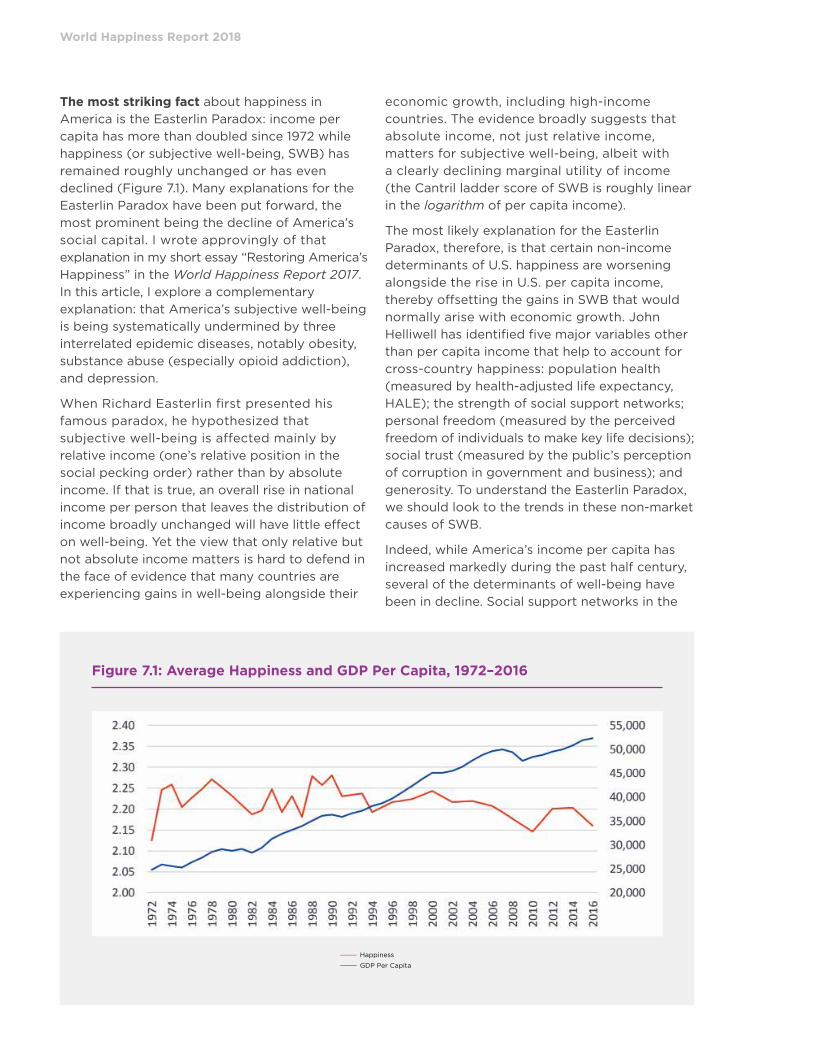
World Happiness Report 2018
The most striking fact about happiness in
America is the Easterlin Paradox: income per
capita has more than doubled since 1972 while
happiness (or subjective well-being, SWB) has
remained roughly unchanged or has even
declined (Figure 7.1). Many explanations for the
Easterlin Paradox have been put forward, the
most prominent being the decline of America’s
social capital. I wrote approvingly of that
explanation in my short essay “Restoring America’s
Happiness” in the World Happiness Report 2017.
In this article, I explore a complementary
explanation: that America’s subjective well-being
is being systematically undermined by three
interrelated epidemic diseases, notably obesity,
substance abuse (especially opioid addiction),
and depression.
When Richard Easterlin first presented his
famous paradox, he hypothesized that
subjective well-being is affected mainly by
relative income (one’s relative position in the
social pecking order) rather than by absolute
income. If that is true, an overall rise in national
income per person that leaves the distribution of
income broadly unchanged will have little effect
on well-being. Yet the view that only relative but
not absolute income matters is hard to defend in
the face of evidence that many countries are
experiencing gains in well-being alongside their
economic growth, including high-income
countries. The evidence broadly suggests that
absolute income, not just relative income,
matters for subjective well-being, albeit with
a clearly declining marginal utility of income
(the Cantril ladder score of SWB is roughly linear
in the logarithm of per capita income).
The most likely explanation for the Easterlin
Paradox, therefore, is that certain non-income
determinants of U.S. happiness are worsening
alongside the rise in U.S. per capita income,
thereby offsetting the gains in SWB that would
normally arise with economic growth. John
Helliwell has identified five major variables other
than per capita income that help to account for
cross-country happiness: population health
(measured by health-adjusted life expectancy,
HALE); the strength of social support networks;
personal freedom (measured by the perceived
freedom of individuals to make key life decisions);
social trust (measured by the public’s perception
of corruption in government and business); and
generosity. To understand the Easterlin Paradox,
we should look to the trends in these non-market
causes of SWB.
Indeed, while America’s income per capita has
increased markedly during the past half century,
several of the determinants of well-being have
been in decline. Social support networks in the
Figure 7.1: Average Happiness and GDP Per Capita, 1972–2016
––––––– Happiness
––––––– GDP Per Capita
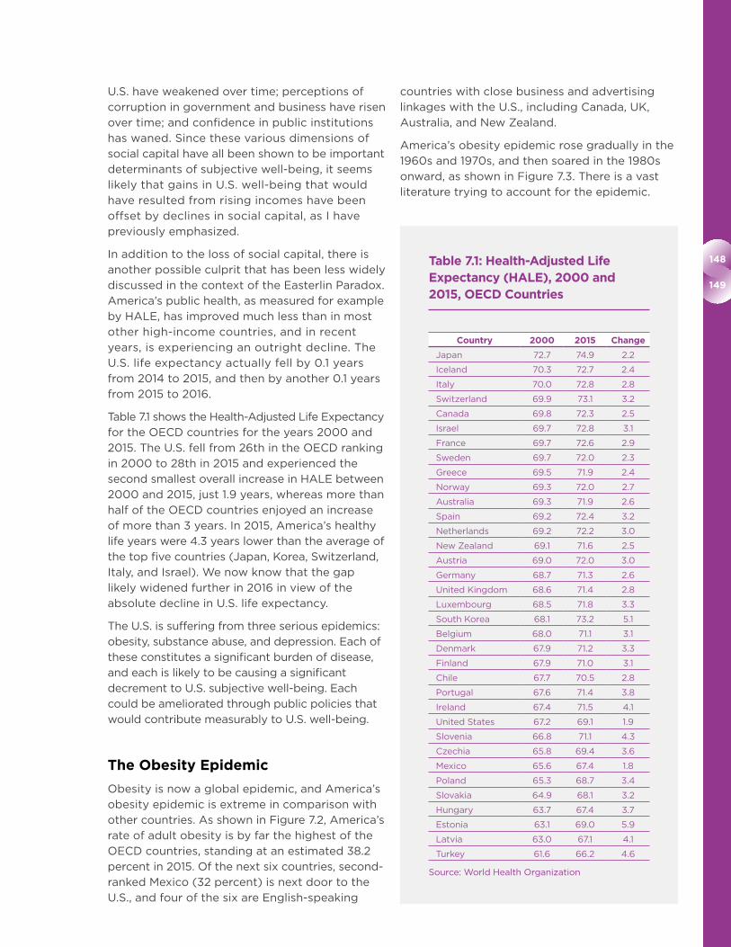
148
149
U.S. have weakened over time; perceptions of
corruption in government and business have risen
over time; and confidence in public institutions
has waned. Since these various dimensions of
social capital have all been shown to be important
determinants of subjective well-being, it seems
likely that gains in U.S. well-being that would
have resulted from rising incomes have been
offset by declines in social capital, as I have
previously emphasized.
In addition to the loss of social capital, there is
another possible culprit that has been less widely
discussed in the context of the Easterlin Paradox.
America’s public health, as measured for example
by HALE, has improved much less than in most
other high-income countries, and in recent
years, is experiencing an outright decline. The
U.S. life expectancy actually fell by 0.1 years
from 2014 to 2015, and then by another 0.1 years
from 2015 to 2016.
Table 7.1 shows the Health-Adjusted Life Expectancy
for the OECD countries for the years 2000 and
2015. The U.S. fell from 26th in the OECD ranking
in 2000 to 28th in 2015 and experienced the
second smallest overall increase in HALE between
2000 and 2015, just 1.9 years, whereas more than
half of the OECD countries enjoyed an increase
of more than 3 years. In 2015, America’s healthy
life years were 4.3 years lower than the average of
the top five countries (Japan, Korea, Switzerland,
Italy, and Israel). We now know that the gap
likely widened further in 2016 in view of the
absolute decline in U.S. life expectancy.
The U.S. is suffering from three serious epidemics:
obesity, substance abuse, and depression. Each of
these constitutes a significant burden of disease,
and each is likely to be causing a significant
decrement to U.S. subjective well-being. Each
could be ameliorated through public policies that
would contribute measurably to U.S. well-being.
The Obesity Epidemic
Obesity is now a global epidemic, and America’s
obesity epidemic is extreme in comparison with
other countries. As shown in Figure 7.2, America’s
rate of adult obesity is by far the highest of the
OECD countries, standing at an estimated 38.2
percent in 2015. Of the next six countries, second-
ranked Mexico (32 percent) is next door to the
U.S., and four of the six are English-speaking
countries with close business and advertising
linkages with the U.S., including Canada, UK,
Australia, and New Zealand.
America’s obesity epidemic rose gradually in the
1960s and 1970s, and then soared in the 1980s
onward, as shown in Figure 7.3. There is a vast
literature trying to account for the epidemic.
Table 7.1: Health-Adjusted Life Expectancy (HALE), 2000 and 2015, OECD Countries
Country 2000 2015 Change
Japan 72.7 74.9 2.2
Iceland 70.3 72.7 2.4
Italy 70.0 72.8 2.8
Switzerland 69.9 73.1 3.2
Canada 69.8 72.3 2.5
Israel 69.7 72.8 3.1
France 69.7 72.6 2.9
Sweden 69.7 72.0 2.3
Greece 69.5 71.9 2.4
Norway 69.3 72.0 2.7
Australia 69.3 71.9 2.6
Spain 69.2 72.4 3.2
Netherlands 69.2 72.2 3.0
New Zealand 69.1 71.6 2.5
Austria 69.0 72.0 3.0
Germany 68.7 71.3 2.6
United Kingdom 68.6 71.4 2.8
Luxembourg 68.5 71.8 3.3
South Korea 68.1 73.2 5.1
Belgium 68.0 71.1 3.1
Denmark 67.9 71.2 3.3
Finland 67.9 71.0 3.1
Chile 67.7 70.5 2.8
Portugal 67.6 71.4 3.8
Ireland 67.4 71.5 4.1
United States 67.2 69.1 1.9
Slovenia 66.8 71.1 4.3
Czechia 65.8 69.4 3.6
Mexico 65.6 67.4 1.8
Poland 65.3 68.7 3.4
Slovakia 64.9 68.1 3.2
Hungary 63.7 67.4 3.7
Estonia 63.1 69.0 5.9
Latvia 63.0 67.1 4.1
Turkey 61.6 66.2 4.6
Source: World Health Organization
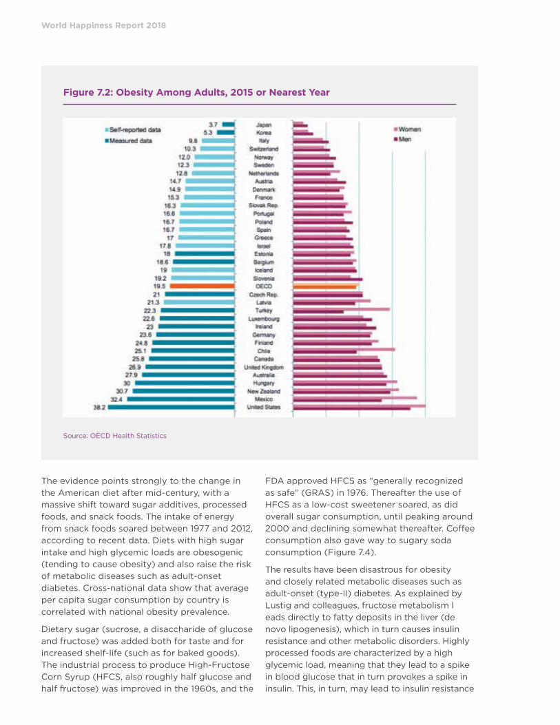
World Happiness Report 2018
The evidence points strongly to the change in
the American diet after mid-century, with a
massive shift toward sugar additives, processed
foods, and snack foods. The intake of energy
from snack foods soared between 1977 and 2012,
according to recent data. Diets with high sugar
intake and high glycemic loads are obesogenic
(tending to cause obesity) and also raise the risk
of metabolic diseases such as adult-onset
diabetes. Cross-national data show that average
per capita sugar consumption by country is
correlated with national obesity prevalence.
Dietary sugar (sucrose, a disaccharide of glucose
and fructose) was added both for taste and for
increased shelf-life (such as for baked goods).
The industrial process to produce High-Fructose
Corn Syrup (HFCS, also roughly half glucose and
half fructose) was improved in the 1960s, and the
FDA approved HFCS as “generally recognized
as safe” (GRAS) in 1976. Thereafter the use of
HFCS as a low-cost sweetener soared, as did
overall sugar consumption, until peaking around
2000 and declining somewhat thereafter. Coffee
consumption also gave way to sugary soda
consumption (Figure 7.4).
The results have been disastrous for obesity
and closely related metabolic diseases such as
adult-onset (type-II) diabetes. As explained by
Lustig and colleagues, fructose metabolism l
eads directly to fatty deposits in the liver (de
novo lipogenesis), which in turn causes insulin
resistance and other metabolic disorders. Highly
processed foods are characterized by a high
glycemic load, meaning that they lead to a spike
in blood glucose that in turn provokes a spike in
insulin. This, in turn, may lead to insulin resistance
Figure 7.2: Obesity Among Adults, 2015 or Nearest Year
Source: OECD Health Statistics
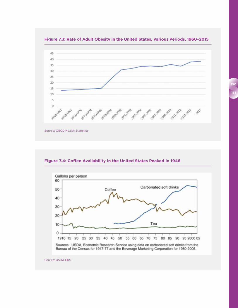
150
151
Figure 7.3: Rate of Adult Obesity in the United States, Various Periods, 1960–2015
Source: OECD Health Statistics
Figure 7.4: Coffee Availability in the United States Peaked in 1946
Source: USDA ERS

World Happiness Report 2018
as well, and metabolic disease. Thus, both high
sugar intake and highly processed foods are
culprits of the obesity epidemic and the accom-
panying epidemic of metabolic disorders.
According to a recent estimate by Euromonitor
International, the U.S. tops the world in the
amount of sugar in purchases of packaged foods
and beverages, with an average of 126 grams per
person per day compared with a global average
at 34 grams per person per day. Of the 126
grams, a remarkable 50 grams comes from soft
drinks alone. Some causes of America’s very high
sugar consumption include: (1) the relatively low
cost per calorie of sugar additives and high
glycemic-load foods compared with foods with
lower glycemic loads such as fruits and vegeta-
bles; (2) the U.S. federal government’s relentless
promotion of corn production from the 1970s
onward, which in turn lowered the cost of
high-fructose corn syrup as a major food additive;
(3) unregulated advertising by the U.S. fast-food
industry to promote prepared, frozen, and
take-out foods with higher sugar content; and
(4) the addictive properties of sugar, leading to
habituation and chronic over-consumption.
Many studies show that obese individuals have
significantly poorer health and lower subjective
well-being. The lower SWB may result both from
the direct health consequences of obesity as well
as the social stigma associated with obesity. The
adverse health consequences are extensive. The
U.S. Centers for Disease Control (CDC) lists the
following adverse disease burdens: all-causes of
death (mortality); high blood pressure (hyperten-
sion); high LDL cholesterol, low HDL cholesterol,
or high levels of triglycerides (dyslipidemia);
type II diabetes; coronary heart disease; stroke;
gallbladder disease; osteoarthritis (a breakdown
of cartilage and bone within a joint); sleep
apnea and breathing problems; some cancers
(endometrial, breast, colon, kidney, gallbladder,
and liver); low quality of life; mental illness such
as clinical depression, anxiety, and other mental
disorders; and body pain and difficulty with
physical functioning.
According to obesity expert Dr. Robert Lustig,
excessive sugar consumption has direct adverse
effects on mental well-being by disrupting the
dopamine-EOP “reward” pathway, causing an
addictive craving for sugar with the classic hall-
marks of addiction (including tolerance, withdrawal,
craving, and continued use despite negative
consequences). Sugar addiction also disrupts the
serotonin pathway that is responsible for the
psychological sense of contentment. In essence,
according to Lustig, sugar is a toxic and addictive
substance that has been dangerously foisted on
an unsuspecting and poorly informed public by
the U.S. government and the fast-food industry.
Studies have found that obesity is a significant
predictive factor for subsequent depression, while
depression is a predictive factor for subsequent
obesity. A meta-analysis of longitudinal studies of
depression and obesity in the U.S. and Europe
reached the following conclusion: “Obesity was
found to increase the risk of depression, most
pronounced among Americans and for clinically
diagnosed depression. In addition, depression
was found to be predictive of developing obesi-
ty.” Lustig describes how interactions between the
dopamine (“reward”) pathways and the serotonin
(“happiness” or “mood”) pathways may account
for this bi-directional linkage between obesity
and depression.
The Opioid Epidemic
In December 2017, the U.S. Centers for Disease
Control announced that U.S. life expectancy had
declined for the second straight year, declining
0.1 years between 2015 to 2016 following a
decline of the same magnitude between 2014
and 2015. This reversal in the upward trend of life
expectancy is shocking and almost unprecedented
for a rich country in recent decades. The CDC
emphasized the role of rising substance abuse,
and especially the modern opioid epidemic, in
the reversal. The CDC counted 63,000 deaths
from drug overdoses in 2016, marking an in-
crease in the age-specific mortality rate from 6.1
per 100,000 in 1999 to 19.8 per 100,000 in 2016,
as shown in Figure 7.5.
While many socioeconomic factors and substances
are involved in this epidemic, one major culprit is
the class of opioids. Causes of increased opioid
deaths include the introduction in the 1990s of
new prescription opioids such as OxyContin, the
update of new powerful synthetic opioids such
as Fentanyl, and the increased use of heroin, with
trends shown in Figure 7.6.
Roughly 20 years after the onset of the opioid
prescription-drug epidemic, it is becoming

152
153
Figure 7.5: Age-adjusted Drug Overdose Death Rates: U.S., 1999–2016
Source: CDC
Figure 7.6: Overdose Deaths Involving Opioids, by Type of Opioid, United States, 2000–2015
Source: CDC
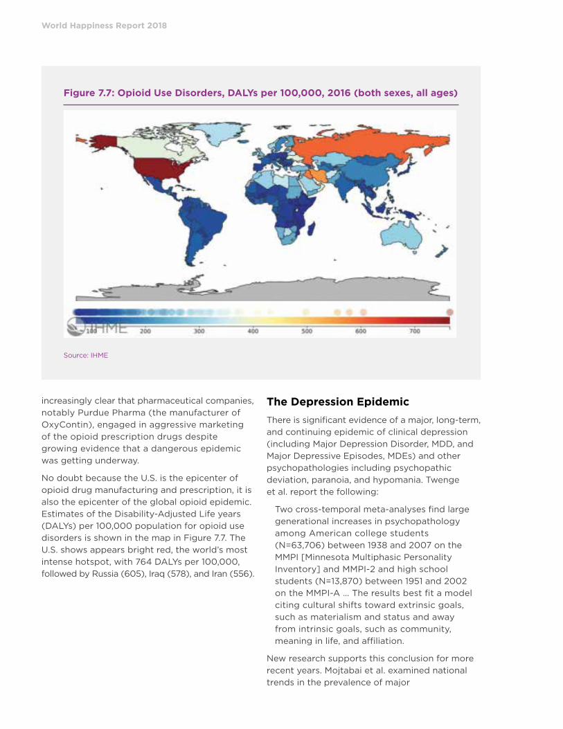
World Happiness Report 2018
increasingly clear that pharmaceutical companies,
notably Purdue Pharma (the manufacturer of
OxyContin), engaged in aggressive marketing
of the opioid prescription drugs despite
growing evidence that a dangerous epidemic
was getting underway.
No doubt because the U.S. is the epicenter of
opioid drug manufacturing and prescription, it is
also the epicenter of the global opioid epidemic.
Estimates of the Disability-Adjusted Life years
(DALYs) per 100,000 population for opioid use
disorders is shown in the map in Figure 7.7. The
U.S. shows appears bright red, the world’s most
intense hotspot, with 764 DALYs per 100,000,
followed by Russia (605), Iraq (578), and Iran (556).
The Depression Epidemic
There is significant evidence of a major, long-term,
and continuing epidemic of clinical depression
(including Major Depression Disorder, MDD, and
Major Depressive Episodes, MDEs) and other
psychopathologies including psychopathic
deviation, paranoia, and hypomania. Twenge
et al. report the following:
Two cross-temporal meta-analyses find large
generational increases in psychopathology
among American college students
(N=63,706) between 1938 and 2007 on the
MMPI [Minnesota Multiphasic Personality
Inventory] and MMPI-2 and high school
students (N=13,870) between 1951 and 2002
on the MMPI-A … The results best fit a model
citing cultural shifts toward extrinsic goals,
such as materialism and status and away
from intrinsic goals, such as community,
meaning in life, and affiliation.
New research supports this conclusion for more
recent years. Mojtabai et al. examined national
trends in the prevalence of major
Figure 7.7: Opioid Use Disorders, DALYs per 100,000, 2016 (both sexes, all ages)
Source: IHME

154
155
depressive episodes (MDEs) in adolescents and
young adults between 2005 and 2014, with the
following conclusions:
The 12-month prevalence of MDEs increased
from 8.7% in 2005 to 11.3% in 2014 in adoles-
cents and from 8.8% to 9.6% in young adults
(both P < .001). The increase was larger and
statistically significant only in the age range of
12 to 20 years. The trends remained significant
after adjustment for substance use disorders
and sociodemographic factors … In the
context of little change in mental health
treatments, trends in prevalence translate
into a growing number of young people with
untreated depression.
Another study this past year reaches a very
similar conclusion:
The current study estimated trends in the
prevalence of major depression in the U.S.
population from 2005 to 2015 overall and by
demographic subgroups. Data were drawn
from the National Survey on Drug Use and
Health (NSDUH), an annual cross-sectional
study of U.S. persons ages 12 and over (total
analytic sample N = 607,520). Depression
prevalence increased significantly in the
U.S. from 2005 to 2015, before and after
controlling for demographics. Increases in
depression were significant for the youngest
and oldest age groups, men, and women,
Non-Hispanic White persons, the lowest
income group, and the highest education and
income groups.
The causes of the MDD epidemic are not defini-
tively established. They may include sociological
factors (decline in social support systems, more
loneliness), economic factors (rising inequality of
income, financial crisis, economic stress), shifting
cultural norms (more materialism), biophysical
factors (declining physical activity, sugar addiction
and other dietary changes, obesity, less time spent
in open sunlight), technological facts (time spent
on social media and electronic devices such as
smartphones), or other causes still to be identified.
As with obesity and opioid abuse, the U.S. stands
out among the world’s nations as having one of
the highest burdens of disease from major
Figure 7.8: Major Depressive Disorder (MDD), DALYs per 100,000, 2016 (both sexes, all ages)
Source: IHME
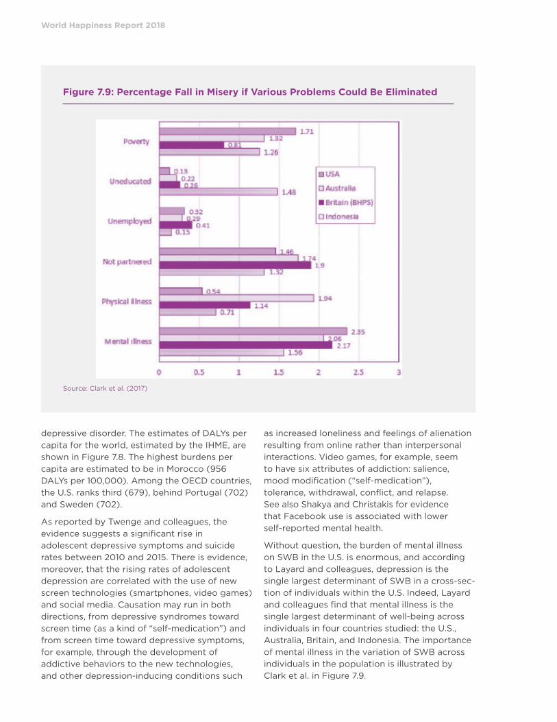
World Happiness Report 2018
depressive disorder. The estimates of DALYs per
capita for the world, estimated by the IHME, are
shown in Figure 7.8. The highest burdens per
capita are estimated to be in Morocco (956
DALYs per 100,000). Among the OECD countries,
the U.S. ranks third (679), behind Portugal (702)
and Sweden (702).
As reported by Twenge and colleagues, the
evidence suggests a significant rise in
adolescent depressive symptoms and suicide
rates between 2010 and 2015. There is evidence,
moreover, that the rising rates of adolescent
depression are correlated with the use of new
screen technologies (smartphones, video games)
and social media. Causation may run in both
directions, from depressive syndromes toward
screen time (as a kind of “self-medication”) and
from screen time toward depressive symptoms,
for example, through the development of
addictive behaviors to the new technologies,
and other depression-inducing conditions such
as increased loneliness and feelings of alienation
resulting from online rather than interpersonal
interactions. Video games, for example, seem
to have six attributes of addiction: salience,
mood modification (“self-medication”),
tolerance, withdrawal, conflict, and relapse.
See also Shakya and Christakis for evidence
that Facebook use is associated with lower
self-reported mental health.
Without question, the burden of mental illness
on SWB in the U.S. is enormous, and according
to Layard and colleagues, depression is the
single largest determinant of SWB in a cross-sec-
tion of individuals within the U.S. Indeed, Layard
and colleagues find that mental illness is the
single largest determinant of well-being across
individuals in four countries studied: the U.S.,
Australia, Britain, and Indonesia. The importance
of mental illness in the variation of SWB across
individuals in the population is illustrated by
Clark et al. in Figure 7.9.
Figure 7.9: Percentage Fall in Misery if Various Problems Could Be Eliminated
Source: Clark et al. (2017)

156
157
Discussion
The U.S. is in the midst of a complex and
worsening public-health crisis, involving
epidemics of obesity, opioid addiction, and major
depressive disorder that are all remarkable by
global standards. The cumulative effect of these
epidemics is the remarkable recent fall in overall
life expectancy at birth (LEB), an event that is
nearly unprecedented for a high-income country
in peacetime. Even before the national LEB
began to decline in 2015, age-specific all-cause
mortality rates were already on the rise between
1999 and 2013 for white, non-Hispanic, working-
class, midlife adults (aged 45-54), notably those
without a college degree, as documented by
Case and Deaton. The major causes of the rising
death rates noted by Case and Deaton were drug
overdoses, suicides, and alcohol-related liver
mortality, consistent with the rising prevalence
of substance abuse (including opioids) and
mental illness.
The quantitative implications of these epidemics
for America’s overall SWB is hard to assess
without more granular data linking individual
SWB with individual conditions of obesity, opioid
dependence, and depression. Yet we are justified
to suspect that the implications are very large.
America’s HALE is now around 4.3 years behind
the five leading countries, and America’s obesity
prevalence, opioid misuse, and MDD prevalence
are among the very highest in the world. As
Layard has recently reminded us:
Mental illness is one of the main causes of
unhappiness in the world. It produces nearly
as much of the misery that exists as poverty
does, and more than is caused by physical
illness. Treating it should be a top priority for
every government, as should the promotion
of good mental health … This would save
billions because mental illness is a major
block on the economy. It is the main illness
among people of working age. It reduces
national income per head by some 5 per
cent—through non-employment, absenteeism,
lowered productivity, and extra physical
healthcare costs. Mental illness accounts for
a third of disability worldwide.
Why has the United States performed more
poorly than other high-income countries on
public health generally, and on these three
epidemics specifically? I would suggest the
following four hypotheses.
First, the U.S. sociopolitical system produces
higher levels of income inequality than in the
other OECD high-income countries. High U.S.
inequality, and especially the persistent
absolute and relative poverty of a significant
portion of the U.S. population, are risk factors
for all three epidemics. The evidence is clear that
low socioeconomic status is a major risk factor
for poor mental and physical health. As Everson
et al. concluded:
Many of the leading causes of death and
disability in the United States and other
countries are associated with socioeconomic
position. The least well-off suffer a dispro-
portionate share of the burden of disease,
including depression, obesity, and diabetes …
Data from these studies demonstrate that
the effects of economic disadvantage are
cumulative, with the greatest risk of poor
mental and physical health seen among
those who experienced sustained hardship
over time.
Second, the three epidemics are mostly likely
mutually reinforcing. Obesity causes depression
and depression can lead to obesity. Depression
and substance abuse are also bi-causal.
Third, the U.S. healthcare system is woefully
inadequate to face these epidemics. U.S. health-
care is the most expensive in the world by far.
Coverage rates of the poor are the lowest among
the high-income countries. The emphasis is on
treatment rather than prevention. And healthcare
for depression is notably deficient. According to
Dr. Renee Goodwin, “A growing number of Amer-
icans, especially socioeconomically vulnerable indi-
viduals and young persons, are suffering from
untreated depression.”
Fourth, America’s culture and politics of
corporate deregulation is partly responsible. The
obesity epidemic can be linked directly to the
fast-food industry, especially the aggressive use
and promotion of sugar additives and other
obesogenic processed foods. The opioid epidemic
can be traced in part to the lobbying and direct
marketing of major pharmaceutical companies.
The extraordinarily high cost, and therefore
under-coverage, of the U.S. healthcare system,
including for mental illnesses, is the result in part

World Happiness Report 2018
of corporate lobbying for the freedom of private
healthcare providers to set exorbitant prices
despite the evidence of very limited and inade-
quate market competition
over prices.
Fifth, the U.S. may be among the leading countries
experiencing depressive syndromes associated
with the new social media and with increasing
screen times on the new ICTs. As indicated
earlier, the correlation of depression and new
media is likely to be bi-causal. Depressive
tendencies may lead to excessive use of new
technologies, while screen time may itself be
addictive and/or linked to increased loneliness
and alienation.
The disease epidemics, in short, most likely have
a similar etiology to the decline in social capital
that I addressed in my analysis in last year’s
World Happiness Report. In both cases, inequali-
ty, corporate power, and disruptions of so-
cial-support networks, are major factors in
America’s social crisis. The result is a decline in
trust, a rise in perceptions of corruption, and a
population that is suffering from pain, suffering,
and premature mortality.
Practical policies exist to reverse all three of
the epidemics. Obesity can be reduced through
regulations limiting sugar additives in store-
bought products; corrective taxes on soda
beverages; the elimination of subsidies on corn
(and therefore on high-fructose corn syrup);
limits on food advertising, especially to young
children; and the promotion of public awareness
regarding the causes of obesity and solution
through more healthful diets. Mental health can
be improved through preventative medicine,
measures to strengthen social support systems
for vulnerable groups, steps to combat addic-
tions to the new social media and technologies,
and greatly improved access to mental health
services. The opioid epidemic could be radically
reduced by ending the direct marketing of addic-
tive drugs to patients as well as banning the
implicit and explicit kickbacks to doctors who
(over-)prescribe these dangerous products.
These are important “top-down” policy changes.
At the same time, “bottom-up” programs of
positive psychology and wellness at schools,
workplaces, and in the community can help
individuals to change their own behaviours,
overcome addictions, and pursue life strategies
(such as meditation) to bolster their personal
well-being and the well-being of friends, family,
and community. The evidence is large and
growing that such life-change strategies can be
highly effective. This year’s Global Happiness Policy Report contains detailed surveys on best
practices in education, the workplace, and
personal, family, and community well-being.
The main issue for the U.S. is not the lack of
means to address the crises of public health and
declining well-being. Rather, perhaps the major
practical barrier is corporate lobbying that keeps
dangerous corporate practices in place and
imposes untold burdens on the poor and
vulnerable parts of the U.S. population, coupled
with the failure of the American political system
to address and understand America’s growing
social crisis. The challenge of well-being is a matter
both of high politics and economics and the sum
of individual and community-based efforts.

158
159
References
Andreassen, C. S., Billieux, J., Griffiths, M. D., Kuss, D. J., Demetrovics, Z., Mazzoni, E., & Pallesen, S. (2016). The relationship between addictive use of social media and video games and symptoms of psychiatric disorders: A large-scale cross-sectional study. Psychology of Addictive Behaviors, 30(2), 252-262. doi: 10.1037/adb0000160
Bandy, L. (2015). Global nutrition overview: Sugar. Euromonitor International. Retrieved from https://blog.euromonitor.com/2015/10/global-nutrition-overview-sugar.html
Case, A., & Deaton, A. (2017). Mortality and morbidity in the 21st century. Brookings Papers on Economic Activity, 397-476. Retrieved from https://www.brookings.edu/wp-content/uploads/2017/08/casetextsp17bpea.pdf
Case, A., & Deaton, A. (2015). Rising morbidity and mortality in midlife among white non-Hispanic Americans in the 21st century. Proceedings of the National Academy of Sciences, 112(49), 15078-15083. doi: 10.1073/pnas.1518393112
Centers for Disease Control and Prevention. (2017). Adult Obesity Causes & Consequences. Overweight & Obesity: Defining Adult Obesity. Retrieved from https://www.cdc.gov/obesity/adult/causes.html
Centers for Disease Control and Prevention. (2017). Opioid data analysis. Opioid Overdose: Data. Retrieved from https://www.cdc.gov/drugoverdose/data/analysis.html
Columbia University, Mailman School of Public Health. (2017). Depression is on the rise in the U.S., especially among young teens. Public Health Now: News. Retrieved from https://www.mailman.columbia.edu/public-health-now/news/depression-rise-us-especially-among-young-teens
Clark, A. E., Fleche, S., Layard, R., Powdthavee, N., & Ward, G. (2017). The key determinants of happiness and misery. In J. Helliwell, R. Layard, & J. Sachs (Eds.), World Happiness Report 2017, 122-142. New York: UN Sustainable Development Solutions Network.
Currie, J. M. (2018). Inequality in mortality over the life course: why things are not as bad as you think. Contemporary Economic Policy, 36(1), 7-23. doi: 10.1111/coep.12267
Dunford, E. K., & Popkin, B. M. (2017). Disparities in snacking trends in us adults over a 35-year period from 1977 to 2012. Nutrients, 9(8), 1-10. doi: 10.3390/nu9080809
Easterlin, R. (1974). Does economic growth improve the human lot? Some empirical evidence. In P. A. David & M. W. Reder (Eds.), Nations and Households in Economic Growth: Essays in Honor of Moses Abramovitz, 89-125. New York: Academic Press.
Everson, S. A., Siobhan, C. M., Lynch, J. W., & Kaplan, G. A. (2002). Epidemiologic evidence for the relation between socioeconomic status and depression, obesity, and diabetes. Journal of Psychosomatic Research 53(4), 891-895. doi: http://dx.doi.org/10.1016/S0022-3999(02)00303-3
Global Happiness Council (2018). Global Happiness Policy Report 2018. New York: Sustainable Development Solutions Network.
Hedegaard, H., Warner, M., & Miniño, A. M. (2017). Drug overdose deaths in the United States, 1999–2016. NCHS Data Brief, (294), 1-8. Retrieved from https://www.cdc.gov/nchs/data/databriefs/db294.pdf
Helliwell, J., Layard, R., & Sachs, J. (2017) Restoring American happiness. In J. Helliwell, R. Layard, & J. Sachs (Eds.), World Happiness Report 2017, 178-184. New York: Sustainable Development Solutions Network.
Helliwell, J., Huang, H., & Wang, S. (2017). Social foundations of world happiness. In J. Helliwell, R. Layard, & J. Sachs (Eds.), World Happiness Report 2017, 8-47. New York: UN Sustainable Development Solutions Network.
Holt-Lunstad, J., Robles, T., & Sbarra, D. A. (2017). Advancing social connection as a public health priority in the United States. American Psychologist, 72(6), 517-530. doi: http://dx.doi.org/10.1037/amp0000103
Holt-Lunstad, J., Smith, T. B., Baker, M., Harris, T., & Stephenson, D. (2015). Loneliness and social isolation as risk factors for mortality: a meta-analytic review. Perspectives on Psychological Science, 10(2), 227-237. doi: https://doi.org/10.1177/1745691614568352
Endnotes
1 Helliwell, Layard, & Sachs (2017).
2 Easterlin (1974).
3 Sachs (2017).
4 Dunford & Popkin (2017); Lustig (2017).
5 Willett (2011); Lustig (2017).
6 Siervo et al. (2014).
7 Lim (2010).
8 Euromonitor International (2015).
9 Lustig (2017).
10 Luppino et al. (2010).
11 Lustig (2017).
12 Keefe (2017).
13 Twenge et al. (2010).
14 Weinberger et al. (2017).
15 Mojtabai et al. (2016).
16 Twenge et al. (2017).
17 Andreassen et al. (2015).
18 Shakya & Christakis (2017).
19 Clark et al. (2017).
20 Case & Deaton (2015, 2017).
21 Layard (2018).
22 Everson et al. (2002).
23 Co-author of Weinberger et al. (2017).
24 Helliwell, Layard, & Sachs (2017).
25 Lai et al. (2017).
26 Willett (2011); Lustig (2017).
27 Layard (2018).
28 Global Happiness Council (2018).
World Happiness Report 2018
IHME. (2017). B.7.4.1: Major depressive disorder, both sexes, all ages, 2016, DALYs per 100,000. GBD Compare: Viz Hub. Retrieved from http://ihmeuw.org/4cn3
IHME. (2017). B.7.3.1: Opioid use disorders, both sexes, all ages, 2016, DALYs per 100,000. GBD Compare: Viz Hub. Retrieved from http://ihmeuw.org/4cn1
Keefe, P. R. (2017). The family that built an empire of pain. The New Yorker. Retrieved from https://www.newyorker.com/magazine/2017/10/30/the-family-that-built-an-empire-of-pain
Kochanek, K. D., Murphy, S. L., Xu, J., & Arias, E. (2017). Mortality in the United States, 2016. NCHS Data Brief, (293), 1-8. Retrieved from https://www.cdc.gov/nchs/data/databriefs/db293.pdf
Lal, A., Mantilla-Herrera, A. M., Veerman, L., Backholer, K., Sacks, G., Moodie, M., Siahpush, M., Carter, R., & Peeters, A. (2017). Modelled health benefits of a sugar-sweetened beverage tax across different socioeconomic groups in Australia: A cost-effectiveness and equity analysis. PLoS Medicine, 14(6), 1-17. doi: 10.1371/journal.pmed.1002326
Layard, R. (2018). Mental illness destroys happiness and is costless to treat. In J. Sachs (Ed.), Global Happiness: Policy Report 2018, 27-52. New York: Sustainable Development Solutions Network.
Lim, J. S., Mietus-Snyder, M., Valente, A., Schwarz, J. M., & Lustig, R. H. (2010). The role of fructose in the pathogenesis of NAFLD and the metabolic syndrome. Nature Reviews Gastroenterology & Hepatology, 7(5), 251-264. doi: 10.1038/nrgastro.2010.41
Luppino, F. S., de Wit, L. M., Bouvy, P. F., Stijnen, T., Cuijpers, P., Penninx, B. W. J. H., & Zitman, F. G. (2010). Overweight, obesity, and depression: A systematic review and meta-analysis of longitudinal studies. Archives of General Psychiatry, 67(3), 220-229. doi: 10.1001/archgenpsychiatry.2010.2
Lustig, R. H. (2017). The Hacking of the American Mind. New York: Avery.
Mojtabai, R., Olfson, M., & Han, B. (2016). National trends in the prevalence and treatment of depression in adolescents and young adults. Pediatrics, 138(6), 1-10. doi: 10.1542/peds.2016-1878 OECD. (2017). Obesity update: 2017. Retrieved from: https://www.oecd.org/els/health-systems/Obesity-Up-date-2017.pdf
Ogden, C. L., & Carroll, M. D. (2010). Prevalence of obesity among children and adolescents: United States, trends 1963-1965 through 2007-2008. National Center for Health Statistics, Centers for Disease Control and Prevention, 1-5. Retrieved from https://www.cdc.gov/nchs/data/hestat/obesity_child_07_08/obesity_child_07_08.pdf
Ogden, C. L., Carroll, M. D., Fryar, C. D., & Flegal, K. M. (2015). Prevalence of obesity among adults and youth: United States, 2011-2014. NCHS Data Brief, (219), 1-8. Retrieved from https://www.cdc.gov/nchs/data/databriefs/db219.pdf
Shakya, H. B., & Christakis, N. A. (2017). Association of Facebook use with compromised well-being: A longitudinal study. American Journal of Epidemiology, 185(3), 203-211. doi: 10.1093/aje/kww189
Siervo, M., Montagnese, C., Mathers, J. C., Soroka, K. R., Stephan, B. C. M, & Wells, J. C. K. (2014). Sugar consumption and global prevalence of obesity and hypertension: An ecological analysis. Public Health Nutrition, 17(3), 587–596. doi: 10.1017/S1368980013000141
Twenge, J. M., Gentile, B., DeWall, C. N., Ma, D., Lacefield, K., & Schurtz, D. R. (2010). Birth cohort increases in psychopathology among young Americans, 1938–2007: A cross-temporal meta-analysis of the MMPI. Clinical Psychology Review, 30(2), 145-154. doi: 10.1016/j.cpr.2009.10.005
Twenge, J. M., Joiner, T. E., Rogers, M. L., & Martin, G. N. (2017). Increases in depressive symptoms, suicide-related outcomes, and suicide rates among U.S. adolescents after 2010 and links to increased new media screen time. Clinical Psychological Science, 6(1), 3-17. doi: https://doi.org/10.1177/2167702617723376
USDA ERS. (2014). Coffee availability in the United States peaked in 1946. Data Products. Retrieved from https://www.ers.usda.gov/data-products/chart-gallery/gallery/chart- detail/?chartId=58921
Weinberger, A. H., Gbedemah, M., Martinez, A. M., Nash, D., Galea, S., & Goodwin, R. D. (2017). Trends in depression prevalence in the USA from 2005 to 2015: Widening disparities in vulnerable groups. Psychological Medicine, 1-10. doi: 10.1017/S0033291717002781
Willett, W. (2011). Eat, Drink, and Be Healthy: The Harvard Medi-cal School Guide to Health Eating. Free Press.

160
161Annex
Migrant Acceptance Index: Do Migrants Have Better Lives in Countries That Accept Them?
Neli Esipova, Julie Ray, John Fleming and Anita Pugliese

World Happiness Report 2018
In reaction to the migrant crisis that swept
Europe in 2015 and the backlash against
migrants that accompanied it, Gallup
developed a Migrant Acceptance Index
(MAI) designed to gauge people’s personal
acceptance of migrants not just in Europe,
but throughout the rest of the world.1
Gallup’s Migrant Acceptance Index is based
on three questions that ask respondents about
migrants in increasing level of proximity to
them. Respondents are asked whether the
following situations are “good things” or
“bad things”: immigrants living in their country,
an immigrant becoming their neighbor and
immigrants marrying into their families.
“A good thing” response is worth three points
in the index calculation, a volunteered response
of “it depends” or “don’t know” is worth one
point, and “a bad thing” is worth zero points.
We considered volunteered responses such as “it
depends” because in some countries, who these
migrants are may factor more heavily into whether
they are accepted. The index is a sum of the
points across the three questions, with a maximum
possible score of 9.0 (all three are good things)
and a minimum possible score of zero (all three
are bad things). The higher the score, the more
accepting the population is of migrants.
Scores on Gallup’s first global deployment of this
index ranged widely across the total 140 countries
where these questions were asked in 2016 and
2017,2 from a high of 8.26 in Iceland to a low of
1.47 in Macedonia. The total sample included more
than 147,000 adults aged 15 and older, and among
them, more than 8,000 first-generation migrants.
In all, 29 countries’ index scores fall more than
one standard deviation below the country-level
mean score and 23 countries’ index scores fall
more than one standard deviation above the
country-level mean score. The bulk of the rest
of the world falls in the middle. In the countries
at the extreme ends of the distribution—the
countries that are the least-accepting and the
most-accepting of migrants – is where we see
the biggest differences in how migrants
themselves rate their lives, which we will discuss
in more detail later.
Least-Accepting Countries Cluster Primarily in Eastern, Southeastern Europe
Many of the countries that are the least-accepting
of migrants are located in Eastern or Southeastern
Europe, and were on the front lines or touched
somehow by the recent migrant crisis. For
example, nine of the 10 countries that score a
2.39 or lower on the index are former Soviet bloc
countries—most located along the Balkan route
that once channeled asylum seekers from Greece
to Germany.
While the bulk of the least-accepting countries
are in Eastern or Southeastern Europe, four are in
the Middle East and North Africa. This includes
Israel, Egypt, Iraq and Jordan. The others are in
Table A1. Migrant Acceptance Index Items
Question Response options*
I would like to ask you some questions about foreign immigrants people who have come to live and work in this country from another country. Please tell me whether you, personally, think each of the following is a good thing or a bad thing? How about:
• Immigrants living in [country name]? • An immigrant becoming your neighbor? • An immigrant marrying one of your close relatives?
A good thing
A bad thing
(It depends)
(Don’t know)
(Refused)
*Responses in parentheses were volunteered by the respondent. Copyright © 2016–2017 Gallup, Inc. All rights reserved.

Asia: Afghanistan and Pakistan in South Asia,
Myanmar and Thailand in Southeast Asia, and
Mongolia in East Asia.
Most-Accepting Countries Span Globe, Income Levels
As opposed to the least-accepting countries,
which are more geographically and culturally
clustered, the most-accepting countries for
migrants are located in disparate parts of the
globe. The top two most-accepting countries
could not be farther apart—Iceland with a score
of 8.26, and New Zealand with a score of 8.25.
The bulk of the most-accepting countries for
migrants primarily come from Oceania, Western
Europe, sub-Saharan Africa and Northern
America. However, a common thread tying many
of the most-accepting countries together is their
long history as receiving countries for migrants.
Although the recent U.S. election was marked by
considerable anti-immigrant rhetoric, the U.S.
ranks among the most-accepting countries with
a score of 7.86. Canada also makes this list, but
scores higher than its neighbor to the south, with
a score of 8.14.
Migrant Acceptance Linked to Migrants’ Evaluations of Their Current, Future Lives
For the past decade, Gallup has asked adults
worldwide to evaluate their lives on the Cantril
Self-Anchoring Striving Scale, where “0”
represents the worst possible life, and “10”
represents the best possible life.3 In our earlier
research, we were able to determine that where
migrants come from, where they go, and how
162
163
Figure A1: Distribution of Migrant Acceptance Index Scores
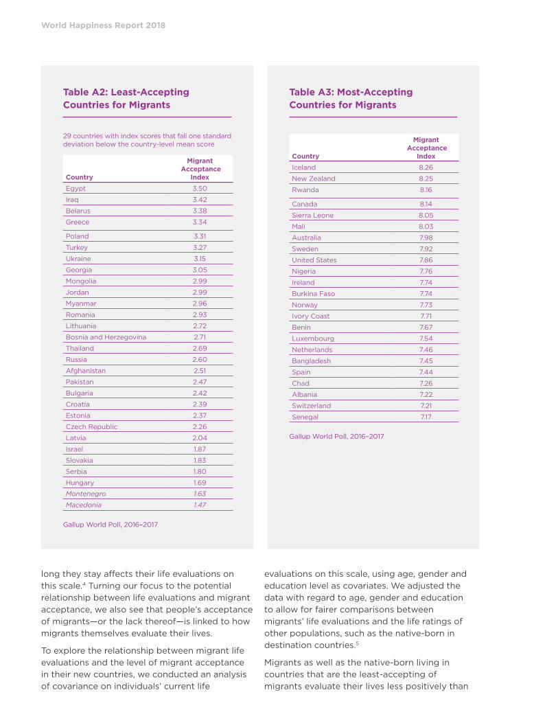
World Happiness Report 2018
long they stay affects their life evaluations on
this scale.4 Turning our focus to the potential
relationship between life evaluations and migrant
acceptance, we also see that people’s acceptance
of migrants—or the lack thereof—is linked to how
migrants themselves evaluate their lives.
To explore the relationship between migrant life
evaluations and the level of migrant acceptance
in their new countries, we conducted an analysis
of covariance on individuals’ current life
evaluations on this scale, using age, gender and
education level as covariates. We adjusted the
data with regard to age, gender and education
to allow for fairer comparisons between
migrants’ life evaluations and the life ratings of
other populations, such as the native-born in
destination countries.5
Migrants as well as the native-born living in
countries that are the least-accepting of
migrants evaluate their lives less positively than
Table A2: Least-Accepting Countries for Migrants
29 countries with index scores that fall one standard deviation below the country-level mean score
Country
Migrant Acceptance
Index
Egypt 3.50
Iraq 3.42
Belarus 3.38
Greece 3.34
Poland 3.31
Turkey 3.27
Ukraine 3.15
Georgia 3.05
Mongolia 2.99
Jordan 2.99
Myanmar 2.96
Romania 2.93
Lithuania 2.72
Bosnia and Herzegovina 2.71
Thailand 2.69
Russia 2.60
Afghanistan 2.51
Pakistan 2.47
Bulgaria 2.42
Croatia 2.39
Estonia 2.37
Czech Republic 2.26
Latvia 2.04
Israel 1.87
Slovakia 1.83
Serbia 1.80
Hungary 1.69
Montenegro 1.63
Macedonia 1.47
Gallup World Poll, 2016–2017
Table A3: Most-Accepting Countries for Migrants
Country
Migrant Acceptance
Index
Iceland 8.26
New Zealand 8.25
Rwanda 8.16
Canada 8.14
Sierra Leone 8.05
Mali 8.03
Australia 7.98
Sweden 7.92
United States 7.86
Nigeria 7.76
Ireland 7.74
Burkina Faso 7.74
Norway 7.73
Ivory Coast 7.71
Benin 7.67
Luxembourg 7.54
Netherlands 7.46
Bangladesh 7.45
Spain 7.44
Chad 7.26
Albania 7.22
Switzerland 7.21
Senegal 7.17
Gallup World Poll, 2016–2017

164
165
those who live in countries that are the most
accepting, regardless of whether they are
newcomers (who have lived in the country for
less than five years) or long-timers (who have
lived in the country for more than five years).6
In the least-accepting countries, newcomers—
who may be full of optimism and hope about life
in their new countries—rate their current lives
more positively than the native-born. But this
positively fades the longer migrants stay in
countries where the population is not receptive
to them. Long-timers’ life evaluations are
statistically much lower than the scores for
newcomers, but their life evaluations also drop
lower than the scores for the native-born.7
The story is different for migrants in the
most-accepting countries. Newcomer migrants
and long-timer migrants both rate their lives
higher than the native-born do. Notably, migrants
do not lose their positive outlook the longer they
stay: The life evaluations of newcomers and
long-timers is statistically the same.
Outlook for the Future
Migrants and the native-born in the least-accepting
countries rate their lives in five years better than
their present situations, but they still lag far
behind their counterparts in the most-accepting
countries. Newcomers in the least-accepting
countries have a more positive outlook for their
lives than the native-born do, but long-timers
again are more pessimistic than either group.
In the most-accepting countries, the native-born
and newcomer migrants share the same level of
optimism about their lives in five years, but
long-timers give their future lives higher ratings
than the native-born or newcomers do. It’s
possible that since long-timers have had more
time than newcomers to establish themselves in
their lives and careers, they not only may be
more hopeful, but also more confident about
what the future may bring.
Figure A2: Current Life Evaluations by Migrant Acceptance Index
Least-accepting countries Most-accepting countries
Gallup World Poll, 2016–2017
8.00
7.00
6.00
5.00
4.00
Native-born Newcomer migrants Long-timer migrants
5.31
6.01
4.87
5.856.33 6.32

World Happiness Report 2018
Future Research
Although Gallup has data from 140 countries, the
samples of migrants available in a single year of
data collection permits us to analyze the links
between migrant acceptance and migrants’ lives
only in broad strokes.
Earlier Gallup research on migrants indicates
that where people come from and where they
move to and how long they stay play a large role
in whether they gain or lose from migration.8
Future World Poll research on migrant acceptance
may allow us not only to do more in-depth
analysis at the country level, but also to discover
whether migrants’ countries of origin also factor
into their life evaluations when they move to
countries that are more likely to accept or to not
accept them. Further, with larger sample sizes,
we would be able to investigate how migrant
acceptance may affect potential migrants’ desire
to migrate and their plans to move and where
they would like to go.
Figure A3: Future Life Evaluations by Migrant Acceptance Index
Least-accepting countries Most-accepting countries
Gallup World Poll, 2016–2017
8.00
7.00
6.00
5.00
4.00
Native-born Newcomer migrants Long-timer migrants
6.436.81
5.74
7.39 7.257.55

166
167
Endnotes
1 Esipova et al (2018).
2 Based on World Poll surveys in 138 countries in 2016, and the U.S. and Canada in 2017.
3 Gallup (2010).
4 International Organization for Migration (2013).
5 Results of the ANCOVA revealed statistically significant effects for two of the three covariates: Education level (F(1,32521) = 2126.5, p < .0001; Gender (F(1,32521) = 23.1, p < .001; and Age (F(1,32521) = 1.9, p < .168).
6 A significant main effect for migrant status emerged with newcomer migrants providing significantly higher life evaluations than either native-born or long-timer migrants, F(2,32521) = 9.0, p < .001. A significant main effect for migrant acceptance also emerged, with respondents from the most-accepting countries providing significantly higher life evaluations than those from the least-accepting countries, F(1,32521) = 60.2, p < .002.
7 A significant Migrant Status x Migrant Acceptance interaction emerged, F(2,32521) = 21.0, p < .001. Simple effects analyses revealed that while newcomer migrants had higher life ratings than their native-born counterparts for both the most- and least-accepting countries, long-tim-er migrants in the least-accepting countries had significant-ly lower life ratings than either the native-born or newcom-er migrants. Long-timer migrants in the most-accepting countries had life evaluations that were equal to those of newcomer migrants.
8 Esipova et al (2013).
References
Esipova, N., Fleming, J., & Ray, J. (2018). New index shows least-, most-accepting countries for migrants. Retrieved from: http://news.gallup.com/poll/216377/new-index-shows-least-ac-cepting-countries-migrants.aspx
Esipova, N., Pugliese, A., & Ray, J. (2013). Worldwide, migrants’ well-being depends on migration path. Retrieved from: http://news.gallup.com/poll/164381/worldwide-migrants-wellbe-ing-depends-migration-path.aspx
Gallup (2010). Understanding how Gallup uses the Cantril scale. Retrieved from: http://news.gallup.com/poll/122453/Understanding-Gallup-Uses-Cantril-Scale.aspx
International Organization for Migration (2013). World migra-tion report 2013: migrant well-being and development. IOM.

World Happiness Report 2018
Edited by John F. Helliwell, Richard Layard and Jeffrey D. Sachs
This publication may be reproduced using the following reference: Helliwell, J., Layard, R., & Sachs, J. (2018). World Happiness Report 2018, New York: Sustainable Development Solutions Network.
World Happiness Report management by Sharon Paculor, copy edit by Claire Bulger, Sybil Fares and Saloni Jain. Design by Stislow Design.
Full text and supporting documentation can be downloaded from the website: http://worldhappiness.report/
#happiness2018
ISBN 978-0-9968513-6-7
The support of the Ernesto Illy Foundation and illycaffè is gratefully acknowledged.
SDSN The Sustainable Development Solutions Network (SDSN) engages scientists, engineers, business and civil society leaders, and development practitioners for evidence-based problem solving. It promotes solutions initiatives that demonstrate the potential of technical and business innovation to support sustainable development.
Sustainable Development Solutions Network 475 Riverside Drive New York, NY 10115 USA