Workspace Modeling and Path Planning for Truss StructureInspection by Unmanned Aircraft

Arun Das∗

Technical University of Munich, 80333 Munich, Germany

and

Craig A. Woolsey†

Virginia Polytechnic Institute and State University, Blacksburg, Virginia 24061

DOI: 10.2514/1.I010634

Small unmanned aircraft systems can increase efficiency and reduce risk to humans during the inspection of truss-

supported structures such as steel bridges. This paper describes a method to mathematically represent a truss and

subsequently to plan an efficient collision-free inspection path. The algorithm checks user-defined perspectives for

feasibility and redefines any infeasible perspectives. A deterministic roadmap is then generated as the complete graph

over these perspectives, and someadditional nodes are generated near the joints of the structure. A traveling salesman

problem (TSP) is solved to find an efficient inspection path that tours all perspective points, and a local A* path

planner then refines the inspection path to circumvent obstructions. The TSP is re-solved, with an updated cost based

on local detours; and the process iterates until a feasibleTSP solution is found.The “lazy” approach to global and local

planning, for which paths are checked for feasibility after the fact and amended if necessary, ensures quick

convergence to an efficient inspection path. Simulation results show the functionality of the algorithm. Comparison

with a probabilistic roadmap method indicates the proposed algorithm’s efficiency.

I. Introduction

W ITH continuing improvements in payload capacity, endurance, and reliability, small unmanned aircraft systems (UASs) have become

helpful tools for aerial mapping, event monitoring, and package delivery. Some UAS proponents have proposed using multicopters to

inspect infrastructure, such as railways, tunnels, and buildings. Bridges are an especially important subset of the public infrastructure. In the

United States, bridgesmust be inspected every two years.Many of these bridges are supported by trusses, which are typically built of steel because

of its strength and resilience; and these trusses feature a large number of welded and bolted connections between beams, girders, and other

structural components that must be routinely examined. The complexity of steel truss bridges and other truss-based structures makes their

inspection time-consuming and expensive because of direct labor and equipment costs and because of indirect costs due to traffic disruptions, for

example. The time, cost, and danger associated with the inspection of truss structures motivate the development of robotic inspection methods.

Previous investigators have proposed various concepts for robotic inspection of steel bridges. These proposals include walking [1], climbing,

and driving robots [2,3] that use magnets, for example, to adhere to the structure. These systems can have difficulty, however, negotiating the

corners, gusset plates, and other structural elements that are peculiar to a truss.We propose the use of a small unmanned aircraft system to inspect

truss-supported structures, such as steel bridges, by flying within the structure and collecting images of user-specified elements.

In preliminary experiments aimed at revealing the challenges associated with aerial robotic bridge inspection, we operated a 3DR Solo

quadcopter under the deck of the George P. ColemanMemorial Bridge in Yorktown, Virginia, in the United States in June 2017; see Figs. 1 and 2.

TheColemanBridge is a 1140-m-long steel bridgewith four lanes for traffic. One span of the bridge is shown in Fig. 1. The deck is supported from

belowby a truss structure, which is built up of seven spans. Two spans in themiddle can rotate 90 deg, parallel to theYorkRiver, thus opening three

lanes for passing ships. The bridgewas originally constructed in 1952 and then rebuilt and widened in 1995. Regular inspection andmaintenance

is performed by the Virginia Department of Transportation.

Themanual flights revealedmajor challenges for truss inspection with UASs. First, electromagnetic disturbances affected the sensing systems.

The Global Positioning System (GPS) signal was unreliable below the bridge deck, and compass measurements were corrupted by the large

amount of steel. Therefore, the positioning capabilities of the UAS were significantly reduced. Second, the pilot had difficulties with flow

disturbances such aswind gusts and turbulence. Thesemade it difficult tomanuallymaintain the aircraft’s position. Lastly, due to the large number

of beams and girders in the structure, the pilot’s view was highly occluded, which made it impossible to conduct flights beyond a short distance

from the pilot. In addition, poor depth perception and distractions such as noise and vibrationsmade themanual operation of a small UASwithin a

truss structure extremely challenging for a human pilot.

The preliminary experiments described previously motivate one to consider automating aerial robotic inspection, although a host of new

challenges arise. For example, the flight control system must effectively compensate for large, unknown wind disturbances; and the navigation

system must operate with unreliable compass and GPS data. Another key element for autonomous inspections is planning the flight path. The

limited endurance ofmultirotorUASs requires short and efficient paths.We propose an algorithm to plan an efficient collision-free inspection path

through a truss structure that obtains inspection images from a number of user-defined perspectives. The focus of this paper is on path planning;

and we defer consideration of other concerns, such as robust flight control, structure-relative navigation, and precision path following. We note

that all of these issues are essential, however, to developing an effective aerial robotic system for truss structure inspection.

Path planning in two dimensions is well studied, and the general methods are reviewed in several comprehensive textbooks [4,5]. Planning in

three dimensions has also enjoyed considerable attention, as described in a recent review by Yang et al. [6]. The authors categorized

Received 14 January 2018; revision received 19 September 2018; accepted for publication 29 October 2018; published online 30 November 2018. Copyright© 2018 byArunDas. Published by theAmerican Institute of Aeronautics andAstronautics, Inc., with permission. All requests for copying and permission to reprintshould be submitted to CCC at www.copyright.com; employ the ISSN 2327-3097 (online) to initiate your request. See also AIAA Rights and Permissionswww.aiaa.org/randp.

*Graduate Student, Electrical Engineering; a.das@tum.de.†Professor, Crofton Department of Aerospace and Ocean Engineering; cwoolsey@vt.edu. Associate Fellow AIAA.

37

JOURNAL OF AEROSPACE INFORMATION SYSTEMS

Vol. 16, No. 1, January 2019

Dow

nloa

ded

by V

IRG

INIA

TEC

H o

n Fe

brua

ry 2

1, 2

019

| http

://ar

c.ai

aa.o

rg |

DO

I: 10

.251

4/1.

I010

634

three-dimenisonal (3-D) planning algorithms into five groups: sampling-based, node-based, mathematical model-based, bioinspired, and

multifusion-based algorithms.Sampling-based algorithms include potential fields, rapidly exploring random trees, probabilistic roadmap algorithms, 3-D Voronoi graphs,

visibility graphs, and corridor maps. These algorithms either produce a path directly or they produce a graph that can be searched for feasiblepaths. Sampling-based methods are widely used because they are well suited for a range of planning applications. Potential field methods assign

repulsive potential functions to obstacles (e.g., to structural elements) and attractive potential functions to goal states. Once the potential field isconstructed, its gradient is easily computed to obtain guidance commands that, in principle, will steer the robot away fromobstructions and toward

the goal. Due to the large number of beams in a truss structure, however, an artificial potential field is likely to produce local minima. Constructinga potential field for a truss structure that guides the aircraft through each of the user-specified vantage points is computationally expensive and

ultimately may not produce a feasible path. Rapidly exploring random trees (RRTs) are often used to quickly generate feasible paths, althoughthey do not produce optimal solutions. Probabilistic roadmap (PRM) approaches are resolution optimal, but a roadmap with a large number of

nodes generally results in large computation times. Results of theRRTandPRMapproaches are illustrated in Figs. 3a and 3b, respectively. Both ofthese probabilistic approaches (the RRTand the PRM) have difficulty finding paths through narrow passages, which is problematic for operationin the confined space within a truss structure. In comparison to the PRM approach, planning methods based on Voronoi graphs emphasize path

safety over path length by maximizing the distance to obstacles.Among sampling-based algorithms, visibility graphs are of particular interest for the application described here. Fig. 3c illustrates path

planning using a visibility graph. Although they are proven to find shortest paths in two dimensions, extending the concept to 3-D produces

connected planes rather than connected lines, resulting in an infinite number of graph nodes. Schøler et al. [7] proposed an alternative extension ofvisibility graphs to 3-D by setting multiple nodes along the edges of obstacles with a specified resolution. To preserve the ability to generateminimum length paths, it would be necessary to set infinitely many nodes along the edges; but, by increasing the resolution, one can trade path

optimality against computation time. Jiang et al. [8] proposed another extension of visibility graphs to 3-D for environments with convex

Fig. 1 George P. Coleman Memorial Bridge.

Fig. 3 Path planning methods in two-dimensional environments with polygonal obstacles. Resulting paths are in red.

Fig. 2 Images from June 2017 flights at the Coleman Memorial Bridge.

38 DAS ANDWOOLSEY

Dow

nloa

ded

by V

IRG

INIA

TEC

H o

n Fe

brua

ry 2

1, 2

019

| http

://ar

c.ai

aa.o

rg |

DO

I: 10

.251

4/1.

I010

634

polygonal obstacles. To overcome the problem of infinitely many nodes, they set a single node at the midpoint of each obstacle edge to serve as apath waypoint and then optimized the path by minimizing a cost function, which moved the waypoints along the obstacle edges. To find theglobally optimum path, all possible edge sequences resulting in feasible paths must be computed and compared. Efficiency decreases withincreasing numbers of obstacles, and the number of possible paths grows exponentially; so, the method’s utility for a large truss structure islimited. Trang et al. [9] proposed an iterative algorithm to compute a shortest path, given a sequence of line segments that might be derived, forexample, using one of the aforementioned methods. Li and Klette [10] analyzed the utility of rubberband algorithms for 3-D path optimization: amethod that can improve grid-based path solutions.

Node-based algorithms are based on graph or map representations, which can be obtained from sampling-based algorithms as described earlieror by directly interrogating the environment. In three dimensions, cubic grids are commonly used, with the cubic grid cells marked as occupied orfree. These are then searched using algorithms such as Dijkstra’s method, A*, Theta*, D*, etc. [11].

Mathematical model-based algorithms (linear programming, optimal control, etc.) can incorporate kinematic and dynamic constraints in thepath planning process, but these approaches are computationally expensive for complex obstacle-filled environments.

Bioinspired algorithms include genetic algorithms, memetic algorithms, particle swarm optimization, ant colony optimization, and neuralnetworks. Thesemethods can iteratively improve an initial solution obtained, for example, using a randomized algorithm. Complex, unstructuredconstraints can be incorporated into path planning, but the algorithms have long iteration times.

Multifusion based algorithms are composed from more basic planning algorithms, enabling one to leverage their relative strengths. Manycombinations exist, which are often targeted at specialized tasks; see Ref. [6].

Path planningmethods targeted toward automated inspection have been proposed for powerlines, railroads, and building exteriors, for example,but these structures present a relatively simple planning challenge in comparisonwith a truss structure.Much of the existingwork on path planningfor robotic inspection of truss structures has focused on robots that remain in contact with the structure as they traverse a path. Liao et al. [12]presented a hierarchical planning algorithm for a climbing robot, for example, inwhichwaypointswere clustered by region and a single inspectionpath was determined for each region. The paths were then connected to form a single, global inspection path. The order in which points werevisited and, more generally, the order in which regions were visited were determined by a traveling salesman problem (TSP) solver.

This paper addresses the problemof efficiently planning a collision-free three-dimensional path through a complex truss structure that enables amultirotor aircraft to image each point feature in a user-specified set from a corresponding user-specified perspective. The approach involvesconstructing a deterministic roadmap, using a three-dimensional variant of the visibility graph, and then iteratively planning over this map tominimize cost while preventing collisions.

Alternatively, onemaywish to survey a structure in its entirety. This objective leads to the problem of path planning for coverage. Galceran andCarreras [13] provided a relatively recent survey of coverage planning tasks and approaches. Although much of the paper focused on two-dimensional planning tasks, one subsection focused on coverage of complex three-dimensional structures, such as the truss structures consideredhere. The authors mentioned the work of Englot and Hover [14], for example, who developed an algorithm for ship hull inspection that firstdetermined points to be visited and then produced a global inspection path. The approachmade iterative use of a TSP solver together with an RRTalgorithm. We adopt a similar procedure in the approach described here.

Bircher et al. [15] proposed a method to automatically compute a set of viewpoints for which the union covered the surface of a structure. Themethod assumed, or extracted, a triangular mesh representation of the structure and computed a single viewpoint for each triangle. A subset ofviewpoints was then selected and a path was planned that visited every viewpoint. Iterative resampling of the viewpoints decreased the path cost.The procedure used a combination of RRTs and a TSP solver, and it ensured that path segments were dynamically feasible.

Our goal is to produce paths that can be followed bymultirotor UASs to inspect truss structures. The various structural elements pose a collisionhazard as the aircraft maneuvers from point to point to obtain inspection images from user-specified perspectives. The planning method mustensure a collision-free path. A multirotor aircraft is preferred because the complexity of a truss structure and the need for high-quality imagerysuggests the need to proceed at a deliberate pace, including the ability to hover. For this reason, and to ensure a time-efficient algorithm,we neglectthe aircraft dynamics in planning inspection paths.

To support the planning method, we introduce a novel way of representing a truss structure. Instead of representing the structure with anoccupancy grid or a detailed mathematical description of the obstacles, we construct a model of simple cuboids using four parameter arrays torepresent the elements of the structure. An advantage of this method is that structures can be modeled with different levels of detail, which areadjusted to the task. Furthermore, computations based on the structure model are efficient because the tessellation contains a relatively smallnumber of triangles: 12 for each modeled beam. The user-defined perspectives are transformed, if necessary, to guarantee that the aircraft canobtain an inspection image along the required boresight direction. The proposed method leaves responsibility for picking viewpoints to theoperator, but any chosen perspectives that are not feasible for the aircraft are automatically transformed to feasible perspectives whilemaintainingthe desired field of view. A roadmap is generated that includes these perspectives along with a collection of “navigation points” that aid pathplanning. The computation of these navigation points is based on the novel way of representing truss structures using a composition of cuboids.The proposedmethod for generating a roadmap can be interpreted as a new adaptation of visibility graphs to 3-D. The resulting roadmap allows forfast path planning because the number of nodes is kept small. Moreover, the method computes short paths, and narrow passages do not pose aproblem. The method incorporates an existing path planning algorithm, such as the A* algorithm, to find a local path between two perspectivesand uses a TSP solver to determine the order in which perspectives are visited. Using a lazy approach allows for fast path planning in large trussstructures.

The algorithm is designed to run offline, as the truss structure to be inspected is assumed to be known a priori. However, computation timeremains an important measure of the algorithm’s performance. In current, commercial infrastructure inspection applications such as powerlineinspection, service providers already optimize their operational procedures tominimize the time required to recover and redeploy an aircraft with afresh battery. Clearly, “time is money” and the ability to quickly replan an inspection path in the field can provide a competitive advantage. For anoperator conducting bridge inspections, it is necessary to be able to replan a path at the scene. For example, a preliminary inspection flightmight bedesigned to quickly survey the entire structure. Based on this first flight, an operator may identify a class or collection of truss components thatrequire further scrutiny.With a fast algorithm, new information can be incorporated at the scene to compute a second inspection path that includesnewly identified problem areas. Our algorithm is optimized to run on the order of minutes rather than days.

The main contributions of this paper are 1) a simplified geometric representation of a truss structure that readily supports path planning; 2) astrategy for transforming infeasible prescribed perspectives into feasible ones; 3) a procedure for computing deterministic navigation points toform a roadmap; 4) an efficient, offline truss structure inspection path planner that iteratively employs a TSP solver and the A* algorithm in a lazyplanning strategy; and 5) parametric studies in the context of a specific inspection scenario aimed at evaluating the proposed method’s efficiencyand effectiveness.

The description of the algorithm in Sec. II through Sec. V is followed by simulation results, which are described in Sec. VI. The paper closeswith concluding remarks in Sec. VII.

DAS ANDWOOLSEY 39

Dow

nloa

ded

by V

IRG

INIA

TEC

H o

n Fe

brua

ry 2

1, 2

019

| http

://ar

c.ai

aa.o

rg |

DO

I: 10

.251

4/1.

I010

634

II. Overview of the Path Planning Algorithm

Our algorithm, which was briefly described in Ref. [16], is based on a new method of representing truss structures for path planning. For thisrepresentation, all components of the truss are enclosed by cuboids. A small set of input parameters is required for the algorithm to compute therepresentation of the structure. In addition to these input parameters, which characterize the truss structure geometry, an operator may definereference perspectives (RPs) that represent UAS configurations (specifying the position and camera boresight direction) at which the aircraftshould obtain images. The algorithm ensures the feasibility of the RPs and relocates them along the specified boresight direction if necessary,resulting in a set of feasible, completely defined amended perspectives (APs).

A deterministic roadmap is then generated using these APs. Additional nodes, called navigation points (NPs), are introduced near the joints ofthe structure that can be adopted as waypoints for local detours to circumvent obstructions along a path between two APs. The use of NPs to aidpath planning is reminiscent of the visibility graph method. The order in which to visit the APs is determined by solving the TSP using a lazymethod that first ignores the possibility that the resulting path might intersect the structure. Thus, initially, the roadmap is the complete graphdefined by all APs andNPs, and the TSP is solved to find an optimal tour that visits everyAP. Path segments are then checked for collisions. Thosesegments that collidewith the structure are removed from the roadmap, and a local A* graph search algorithm computes an alternative local path,resulting in a modified inspection path and a new traversal cost associated with each local detour between APs. The global TSP is then re-solvedusing this modified inspection path as the initial guess and using the modified cost information.

Figure 4 shows a flowchart for the algorithm that proceeds in three major phases, described in Secs. III through V, respectively.

III. Phase 1: Representing the Structure

In the first phase, the structure is defined within the computational environment, as indicated in Fig. 5a for a simple example. We introduce amethod tomathematically represent a truss structure. Themethod enables one to compute occupied and free regions within the environment froma small set of input parameters that describe the geometry of the structure. A truss structure is constructed from many different parts includingbeams, braces, girders, stiffeners, pillars, cables, sway bars, etc. In modeling for path planning, every such element is enclosed by a cuboid.Multiple elements that are densely packed within a volume may be grouped together and enclosed in a single cuboid. It is not necessary todistinguish the individual properties of different components; we treat the cuboids as standardized objects that represent obstructions within theworkspace.We refer to these cuboids as beams andwe call the junctionswhere beams connect joints. Although a given cuboidwill often enclose atrue beam within the structure, it might also enclose some other element, such as a cable or a walkway.

Because the planning algorithm assumes that the UAS is a particle, we expand the volume that is inaccessible to the aircraft by artificiallyincreasing the size of the cuboids defining the structure through a process called inflation; see Fig. 5b. The risk of collisions can be further reduced(to account for position uncertainty or ambient disturbances, for example) by inflating the structure even further. Upon completion of this step, theworkspace is divided into occupied regions and their complement, which are regions that are freely accessible to the aircraft.

A. Coordinate Frames

Tomodel the truss structure, we define two types of reference frame: a single, arbitraryworld frame (subscript 0) and a beam frame (subscript b)for each beam in the structure. The beam frames are needed to parameterize the truss structure in order to compute paths. The originOb of a givenbeam frame is located at one of the beam’s joints, known as the “start joint,” and the z axis of the frame points toward the other joint, known as the“end joint.” This definition is illustrated in Fig. 6, in whichpstart andpend define the position of the beam’s start and end joints, respectively. The xaxis is defined by taking the cross product of the unit vectors defining the z axis of theworld frame and the z axis of the beam frame, according toEq. (2). In case the cross product is zero, xb is chosen equal to the unit vector y0. To obtain a right-handed coordinate system, yb is determined as inEq. (3):

zb � �pend − pstart�∕kpend − pstartk (1)

Representing theStructure

Searching for theInspection Path

Building theRoadmap

StructureMatrices

Ja, Ji, Ba, Bi

InflateStructure

Solve TSP

Obtain theRoadmap

by Connecting all APs and NPs

yes

no

Collision?

Path Planning Algorithm

ComputeStructure

ComputeNavigation

Points (NPs)

ComputeAmended

Perspectives(APs)

ReferencePerspectives

PR

Replace CollidingPath Segments

with FeasiblePath (A*)

Inspection Path,Visiting all APs

Fig. 4 Block diagram of the path planning algorithm with its three phases.

40 DAS ANDWOOLSEY

Dow

nloa

ded

by V

IRG

INIA

TEC

H o

n Fe

brua

ry 2

1, 2

019

| http

://ar

c.ai

aa.o

rg |

DO

I: 10

.251

4/1.

I010

634

xb �� �z0 × zb�∕kz0 × zbk if z0 × zb ≠ 0y0 otherwise

(2)

yb � �zb × xb�∕kzb × xbk (3)

B. Algorithm Inputs: Representing the Structure

The positions of the joints and other parameters of the beams must be provided as input to the structure-modeling algorithm. The joints aredefined by their Cartesian coordinates given in theworld frame. For beams, which are simple cuboids, six parameters are necessary: the indices ofthe start jointnstart;k and end jointnend;k, the beam’s cross-sectional dimensions xsize;k and ysize;k, and possibly offsets xoffset;k and yoffset;k. The cross-sectional dimensions xsize;k and ysize;k must be greater than zero. The offset, specified in the beam frame, allows for the case inwhich the centerlineof a beam does not pass through the start and end joints.

Beyond the geometric parameters introduced earlier, we define a binary classification of joints and beams as either active or inactive. Somebeams are unlikely to affect path planning. A beam at the workspace boundary with no nearby RPs, for example, is unlikely to impede theinspection of other parts of the structure, although it does obstruct theworkspace. Classifying a component as inactive prevents the algorithm frompopulating the roadmap with NPs associated with this component, thereby reducing computation time.

Table 1 lists four arrays labeledJa,Ji,Ba, andBi, which contain the geometric information needed to represent the truss structure in support ofpath planning. Each of these arrays contains a number of elements that define the essential features of the structure.

C. Algorithm Inputs: Representing the Reference Perspectives

RPs specify the desired configurations fromwhich theUAS should obtain images. ThemthRP is defined by a positionpRP;m in theworld frame,and possibly a corresponding boresight direction vRP;m along which the imaging sensor should be aligned. RPs are provided to the algorithm in afifth input array PRP.

When inspecting a bridge, for example, an inspector typically knows in advance about potential problem areas that require attention. Therefore,it is left to the inspector to manually set the RPs, including the viewing angle and the distance to the structure for a desired image. These RPs neednot be chosen in obstacle-free space; the algorithm transforms infeasible RPs into APs. Note that the input arrayPRP could also be provided by anautomated algorithm (e.g., to obtain complete surface coverage).

D. Defining the Structure from Input Parameters

With the input parameters described previously, the algorithm is able to compute the eight vertices vi for i ∈ f1; 2; : : : ; 8g for each beam withrespect to the beam frame. Figure 6 shows a beamwith its beam frame, parameters, and vertices. The coordinates of the first vertex v1 with respectto the beam frame are

Fig. 6 Beam with corresponding parameters and vertices.

Table 1 Structure inputs for the algorithm

Array Description Elements of Given Array

Ja Positions of active joints pactiveJoint;i

Ji Positions of inactive joints pinactiveJoint;j

Ba Parameters for active beams nstart;k, nend;k, xsize;k, ysize;k, xoffset;k, yoffset;kBi Parameters for inactive beams nstart;l, nend;l, xsize;l, ysize;l, xoffset;l, yoffset;l

Fig. 5 Steps of the path planning algorithm.

DAS ANDWOOLSEY 41

Dow

nloa

ded

by V

IRG

INIA

TEC

H o

n Fe

brua

ry 2

1, 2

019

| http

://ar

c.ai

aa.o

rg |

DO

I: 10

.251

4/1.

I010

634

v1 �

0BB@− 1

2xsize � xoffset

12ysize � yoffset

0

1CCA (4)

The remaining three vertices adjacent to the beam’s starting joint are computed analogously to the first. The vertices adjacent to the beam’s endpoint (on the right side in Fig. 6) are computed similarly, but they have the z value kpend − pstartk.

After computing the vertices with respect to the beam frame, they are transformed into the world frame by applying the homogeneoustransformation:

0Tb�vi� � � xb yb zb �vi � pstart (5)

Given the computed vertices, an object for each beam is created in the world frame. The structure is obtained by aggregating allsuch objects.

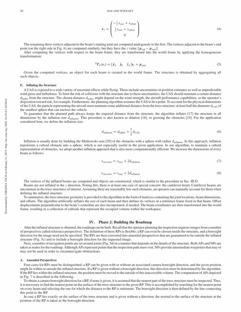
E. Inflating the Structure

AUAS is exposed to a wide variety of uncertain effects while flying. These include uncertainties in position estimates as well as unpredictablewind gusts and turbulence. To limit the risk of collisions with the structure due to these uncertainties, the UAS should maintain a certain distancedbuffer from the structure. The chosen distance dbuffer might depend on the wind strength, the aircraft performance capabilities, or the operator’sdisposition toward risk, for example. Furthermore, the planning algorithm assumes the UAS to be a point. To account for the physical dimensionsof the UAS, the particle representing the aircraft must maintain some additional distance from the truss structure: at least half the diameter dUAS ofthe smallest sphere that can enclose the vehicle.

To guarantee that the planned path always keeps the required distance from the structure, the algorithm inflates [17] the structure in alldimensions by the inflation size dinflation. This procedure is also known as dilation [18], or growing the obstacles [19]. For the applicationconsidered here, we define the inflation size:

dinflation � dbuffer �1

2dUAS (6)

Inflation is usually done by building the Minkowski sum [20] of the obstacles with a sphere with radius dinflation. In this approach, inflationtransforms a cuboid obstacle into a sphere, which is not especially useful in the given application. In our algorithm, to maintain a cuboidrepresentation of obstacles, we adopt another inflation approach that is also more computationally efficient. We increase the dimensions of everybeam as follows:

xsize;new � xsize � 2dinflation (7)

ysize;new � ysize � 2dinflation (8)

The vertices of the inflated beams are computed and objects are constructed, which is similar to the procedure in Sec. III.D.Beams are not inflated in the z direction. Noting this, there is at least one case of special concern: the cantilever beam. Cantilever beams are

uncommon in the truss structures of interest. Assuming there are reasonably few such elements, an operator canmanually account for themwhendefining the inflated structure.

To summarize, the truss structure geometry is provided to the algorithm in the formofmatrices containing the joint locations, beamdimensions,and offsets. The algorithm artificially inflates the size of each beam and then defines its vertices in a reference frame fixed in that beam. Offsetdisplacements perpendicular to the beam’s centerline are also incorporated, if needed. The beam coordinates are then transformed into the worldframe, resulting in a collection of cuboids that represent the occupied volume within the workspace.

IV. Phase 2: Building the Roadmap

After the inflated structure is obtained, the roadmap can be built. Recall that the operator planning the inspection requests images from a numberof perspectives called reference perspectives. The definition of these RPs is flexible; a RP can even be chosen inside the structure, and a boresightdirection for the image need not be specified. The RPs are then converted into amended perspectives that are guaranteed to lie outside the inflatedstructure (Fig. 5c) and to include a boresight direction for the requested image.

Next, a number of navigation points are set around joints (Fig. 5d) in amanner that depends on the details of the structure. BothAPs andNPs aretaken as nodes for the roadmap.AlthoughAPs represent points that the inspection pathmust visit, NPs provide intermediatewaypoints thatmay ormay not be used in order to circumnavigate obstructions.

A. Amended Perspectives

Four cases for RPs must be distinguished: a RP can be given with or without an associated camera boresight direction, and the given positionmight liewithin or outside the inflated structure. If a RP is givenwithout a boresight direction, this directionmust be determined by the algorithm.If the RP lies within the inflated structure, the positionmust bemoved to the outside of this inaccessible volume. The computation of APs depictedin Fig. 7 is described in the following.

To obtain a camera boresight direction for a RP, if none is given, it is assumed that the nearest part of the truss structuremust be inspected. Thus,it is necessary to find the nearest point on the surface of the truss structure to the given RP. This is accomplished by searching for the nearest pointon every beam and selecting the one for which the distance to the RP is minimum. The boresight direction is then defined by the line connectingthis point to the RP.

In case a RP lies exactly on the surface of the truss structure and is given without a direction, the normal to the surface of the structure at theposition of the RP is taken as the boresight direction.

42 DAS ANDWOOLSEY

Dow

nloa

ded

by V

IRG

INIA

TEC

H o

n Fe

brua

ry 2

1, 2

019

| http

://ar

c.ai

aa.o

rg |

DO

I: 10

.251

4/1.

I010

634

Collision checks are performed to determine if RPs lie inside or outside the inflated structure. If the RP lies outside the structure, it can directly

be taken as anAP.Otherwise, if the RP lies inside the inflated structure, it must bemoved into the accessibleworkspace. A straightforwardmethod

would be to find the nearest point to the RP on the inflated structure and define this as an AP. The RP would be moved in some direction that

depends on its relative position to the truss structure. If the RP ismoved off of the boresight axis, one cannot guarantee the desired component will

remain in the field of view. To avoid this issue, the RP may only move along the boresight axis until it emerges from the inflated structure. This

ensures that the perspective angle and the center of the field of view for the resulting image remain unchanged. Furthermore, if the camera has a

zoom capability, the original field of view can be restored, although other issues could adversely affect image quality, such as platformmotion or

lighting conditions.

B. Navigation Points

NPs are computed relative to the joints connecting beams; only active joints and beams are considered in this step. The essential idea is to

identify the “corner” between intersecting beams and to set NPs at both sides of this corner as shown in Fig. 8a.Note that, if a beam is rotated about its centerline, NPs do not need to lie on the surface of the inflated structure; see Fig. 8b. This is in contrast to

visibility graphs, for which waypoints always lie on the surface of an obstacle. Another special case that the algorithm accommodates is that of

abutted beams with differing cross sections, as shown in Fig. 8c. The computation of NPs is described further in the Appendix.After computing all NPs for each pair of active beams at each active joint, a collision check is performed for all computed NPs to determine if

they lie inside or outside the inflated structure. Points inside the structure are deleted; only those points in the freeworkspace are incorporated into

the roadmap. Figure 9 illustrates the resulting NPs for an example joint with four beams.

V. Phase 3: Planning the Path

The requirement that the inspection path efficiently visit every AP leads to a TSP. The search for the inspection path proceeds iteratively in two

stages. First, a global path planner solves a TSP to determine a tour that visits every AP (Fig. 5e). A local path planner then generates a detour

around obstructionswhere the global path intersects the inflated structure (Fig. 5f). Each infeasible path segment is removed from the roadmap, the

cost of the corresponding detour is tabulated, and the two stages are repeated. The iterative process stops once a TSP solutionwithout collisions is

found. This approach, in which a path is first obtained and then checked for collisions, is often referred to as a lazy method [21].

A. Planning the Global Path

The initial roadmap is defined as the complete graph over all APs and NPs, without performing any collision checks. Our objective is to

minimize the distance traveled by the UAS, rather than to reduce risk, energy, or time, although one could easily accommodate alternative

optimization criteria. Accordingly, theweights of the edgeswithin the roadmap are initializedwith the Euclidean distances between the nodes. An

Referenceperspectives

Yes

No

inside the inflatedstructure?

Yes

No

direction given?

Amendedperspective

= RP + direction

Amendedperspective

= moved RP +direction

Move RP outsidethe inflated

structure in theindicated direction

Find nearest point onthe bridge structure

and compute direction

Fig. 7 Block diagram for the computation of amended perspectives.

2000-500

0

1000500

500

0

1000

0

z (H

eigh

t)

-500

1500

2000

2500

Inflated Truss StructureNavigation PointsIntersection Point

a) Right-angled beams

-500

2000

0

500

1000

z (H

eigh

t)

1000

1500

y (Width)

y (Width)

2000

2500

0 2000

x (Length)x (Length) 1000

0

b) Rotated beams

40003000

x (Length)

2000

-500

0

500 1000

z (H

eigh

t) 500

y (Width)

00-500

c) Beams in the same directionFig. 8 Navigation point examples for different combinations of beams.

DAS ANDWOOLSEY 43

Dow

nloa

ded

by V

IRG

INIA

TEC

H o

n Fe

brua

ry 2

1, 2

019

| http

://ar

c.ai

aa.o

rg |

DO

I: 10

.251

4/1.

I010

634

initial cost matrix C associated with the TSP is set up containing the distance between every pair of APs [22]. Based on the cost matrix C, a TSPsolver determines the order in which the APs should be visited to minimize the total path length.

We use the Lin–Kernighan–Helsgaun (LKH) heuristic [22] as the TSP solver. Although the solution is not guaranteed to be optimal, the solvergenerates a feasible path in reasonable time, even for large numbers of APs. The inspection path determined in this way is then checked forcollisions with the inflated structure. For each path segment that collides with the inflated structure, a local path planner described in the nextsubsection generates a feasible, local, alternative path that incorporates NPs aswaypoints. Because the length of this detour differs from the lengthof the infeasible segment, the cost matrix C is updated and a revised TSP is solved. This iterative process is run until the TSP solver returns afeasible inspection path. The process is depicted in the block diagram in Fig. 10. A similar method for the global path planner was used by Englotand Hover [14] for ship hull inspections.

Path segments that have already been verified as feasible, including local detours generated in response to collisions, are not rechecked forfeasibility in later iterations. Moreover, a prior solution is available to the LKH solver in subsequent iterations, which further accelerates solutionof the modified TSPs.

Remark: Rather than define a single, required perspective for each inspection point, one may prescribe a set of acceptable perspectives fromwhich a single perspective may be selected, as is convenient. Such a set might include all the perspectives fromwhich a given structural feature ofinterest is visible. In solving a generalized TSP (GTSP), one perspective from each set is chosen so that the resulting inspection path is as short aspossible [23]. Although the additional planning freedommay be helpful, the problem requires amodified solutionmethod. Smith and Imeson [24]proposed a GTSP solver called Generalized Large Neighborhood Search (GLNS), for example. We assume, however, that every user-specifiedperspective must be visited, and we apply the more efficient LKH solver to the resulting TSP.

B. Planning Local Paths

The local path planner provides a feasible alternative path connecting two APs in cases in which the straight connecting path collides with theinflated structure. NPs are used as waypoints to circumvent the obstruction.

An implementation of the A* graph search algorithm serves as the local path planner. The algorithm searches the roadmap, which is initiallybuilt by assuming that every edge in the complete graph is feasible and which is amended as infeasible segments are identified within proposedpaths. A block diagram of the process is shown in Fig. 11.

Fig. 10 Block diagram of the global path planning.

Fig. 9 NPs for a joint with multiple beams.

roadmap,APstart, APgoal

A* graphsearch

no

yes

collision?

update roadmap:delete colliding

edges

connecting pathbetween APstart

and APgoal

Fig. 11 Block diagram of the local path planning.

44 DAS ANDWOOLSEY

Dow

nloa

ded

by V

IRG

INIA

TEC

H o

n Fe

brua

ry 2

1, 2

019

| http

://ar

c.ai

aa.o

rg |

DO

I: 10

.251

4/1.

I010

634

VI. Simulations

This section describes simulation results for a half-span of the Coleman Bridge shown in Fig. 1. All simulations were conducted on a computer

with an Intel Core i7-6500U 2.5 GHz processor runningWindows 10. The algorithm was implemented in MATLAB. It should be noted that the

algorithm was not yet optimized in terms of runtime. An optimized implementation in a low-level programming language, possibly using

multithreading, would undoubtedly yield a significant increase in performance.

A. Model of the Coleman Memorial Bridge

Referring to Fig. 1, one can see that the ColemanBridge exhibits a repeating pattern of structural assemblies so that, for path planning purposes,

it is not necessary to model the entire structure. The red box in Fig. 1 indicates the assembly that was modeled here, as shown in Fig. 12.

Referring to Sec. III, themodel comprises 33 active joints, 18 inactive joints, 104 active beams, and 4 inactive beams. The joints at x � −11;000and x � 66;000 are inactive, and so no NPs are set there. Furthermore, the pillar, the deck, and the catwalks are modeled using inactive joints and

inactive beams. For this model, the algorithm automatically sets 694 NPs in the structure, which are visualized on the inflated structure in Fig. 12.

Despite this rather simplistic modeling of the assembly, the representation enables accurate planning of collision-free paths through the structure.

Joints are of particular interest during inspections because they are regions of concentrated stress in which corrosion or cracks are of particular

concern.Accordingly,we defined theRPs around the joints of the structure. Each joint is inspected from at least two sides. Jointswhere inner cross

bracing is connected are inspected from three different angles. This results in a total of 82 defined RPs, of which 28 include no specified boresight

direction. For an inflation size of dinflation � 1000 mm, the resulting path through the noninflated structure is shown in Fig. 13.

B. Dependence on Inflation Size

The inflation size parameter may be adjusted by the operator to allow for a larger or smaller aircraft, to accommodate operations in stronger or

weaker disturbances, etc. It is consequently of interest to know how the computation time and path length vary with inflation size.

The computation times and path lengths for simulations with different inflation sizes are summarized in Table 2 and in Fig. 14. Table 2 also

contains the numbers of solved TSPs, planned local paths, and executed collision checks. The maximum applied inflation size is 2000 mm.

For values larger than this, the inner cross bracing in the middle of the span inflates into a solid obstruction and some RPs become

unreachable.

In general, Fig. 14 suggests that an increasing inflation size corresponds to an increase in computation time and path length. The trend is not

monotonic, however. For example, although the algorithm runs for 472 s for an inflation size of 750 mm, it only takes 419 s when the structure is

inflated by 1000mm.Although the trend in path length appearsmore consistent, the inspection path for the 2000mminflated bridge is 6%shorter than

it is for a 1500mminflation size. This observation likely relates to the fact that the accessible volumewithin the structure (i.e., the availableworkspace)

decreases with larger inflation sizes. Thus, APs within the bridge structure will lie closer together, resulting in a shorter inspection path length.

Fig. 13 Coleman Bridge model with a computed path in red (axis units are in millimeters).

Fig. 12 Navigation points in the inflated Coleman Bridge model (GCB) (axis units are in millimeters).

DAS ANDWOOLSEY 45

Dow

nloa

ded

by V

IRG

INIA

TEC

H o

n Fe

brua

ry 2

1, 2

019

| http

://ar

c.ai

aa.o

rg |

DO

I: 10

.251

4/1.

I010

634

C. Computation Time Distribution

Figure 15 shows the distribution of computation time among the different steps of the algorithm. The distribution that is presented is

averaged among all the inflation sizes dinflation listed in Table 2. The initial computations to obtain the bridge structure, APs, and NPs account

for less than 1% of the algorithm’s total runtime. More than 99% of the runtime is spent searching for the inspection path. When searching for

the inspection path, planning local paths is the costliest task (79% of total runtime), followed by the collision checks for global and local paths

(18% of total runtime). This observation justifies our effort to keep the number of NPs small, thus reducing the size of the roadmap. Also, the

advantage of lazy approaches for global and local path planning is evident. Without lazy path planning, more local path plannings (up to 3321

local paths for the 82APs) withmore collision checks would be required in order to reduce the global path planning effort to a single solution of

the TSP.

Given the computational time spent on local path planning, a reasonable objective for future efforts would be to increase the efficiency of this

step. Algorithms like the D* algorithm can handle changes in the roadmap without the need to start over when an edge is removed from the graph

due to a detected collision.

If the local path planner’s efficiency can be significantly increased, the iterative procedurewould no longer be necessary. In this case, every local

path between APs could be computed in advance and onewould only need to solve a single TSP. The question of which method is more efficient

would depend on the performance of the local path planner as well as that of the TSP solver.

D. Development over Iterations

In the third phase, the algorithm plans the inspection path. This is done iteratively where, in each iteration, a TSP is solved, collision checks are

performed, and local paths are planned. Solving the first TSP instance and finding local paths in the first iteration of the routine take themost time.

From the second iteration on, the TSP solver takes the previous solution as the initial tour, which speeds up the solution process. Also, the number

of planned local paths decreases so that, in general, subsequent iterations will take significantly less time as compared with the first iteration.

Iterations end when a TSP solution without collisions is found. Figure 16 shows the improvements in path length as compared to the previous

iteration (top plot) and the time for the iterations (bottom plot). The improvements are given in percentages compared with the prior iteration. The

plots start at the second iteration because no prior value exists for comparison at the first iteration.

The average improvement in path lengthmade in a single iteration is 0.73%with a standard deviation of 1.45%. Themean computation time per

iteration is 29 s with a standard deviation of 45 s. Again, only a general and imperfect trend can be observed, suggesting that later iterations take

Table 2 Path planning algorithm results for different inflation sizes dinflation

Inflation size dinflation, mm

2 250 500 750 1,000 1,500 2,000

No. of solved TSP instances 5 5 7 10 9 10 34No. of local path plannings 88 95 120 134 141 178 276No. of line collision checks 3,813 6,562 11,668 14,565 13,571 18,965 44,958Computation time, s 125 182 371 472 419 785 2,965Path length, m 360 396 443 489 526 650 613

0 500 1000 1500 2000

Inflation Size [mm]

0

200

400

600

800

1000

Run

time

[s] /

Pat

h Le

ngth

[m]

Algorithm RuntimeInspection Path Length

Fig. 14 Algorithm runtime (blue) and inspection path length (red) versus on the inflation size.

Fig. 15 Time distribution among the steps of the algorithm, averaged for inflation sizes between 2 and 2000 mm.

46 DAS ANDWOOLSEY

Dow

nloa

ded

by V

IRG

INIA

TEC

H o

n Fe

brua

ry 2

1, 2

019

| http

://ar

c.ai

aa.o

rg |

DO

I: 10

.251

4/1.

I010

634

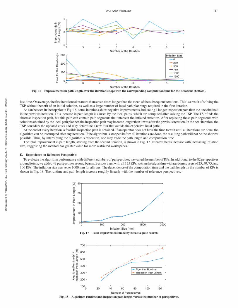
less time.On average, the first iteration takesmore than seven times longer than themean of the subsequent iterations. This is a result of solving the

TSP without benefit of an initial solution, as well as a large number of local path plannings required in the first iteration.

As can be seen in the top plot in Fig. 16, some iterations show negative improvements, indicating a longer inspection path than the one obtained

in the previous iteration. This increase in path length is caused by the local paths, which are computed after solving the TSP. The TSP finds the

shortest inspection path, but this path can contain path segments that intersect the inflated structure. After replacing these path segments with

solutions obtained by the local path planner, the inspection pathmay become longer than it was after the previous iteration. In the next iteration, the

TSP considers the updated costs and may determine a new tour that avoids the expensive local paths.

At the end of every iteration, a feasible inspection path is obtained. If an operator does not have the time towait until all iterations are done, the

algorithm can be interrupted after any iteration. If the algorithm is stopped before all iterations are done, the resulting path will not be the shortest

possible. Thus, by interrupting the algorithm’s execution, one may trade the path length and computation time.

The total improvement in path length, starting from the second iteration, is shown in Fig. 17. Improvements increase with increasing inflation

size, suggesting the method has greater value for more restricted workspaces.

E. Dependence on Reference Perspectives

To evaluate the algorithm performancewith different numbers of perspectives, wevaried the number of RPs. In additional to the 82 perspectives

around joints, we added 43 perspectives around beams. Besides a runwith all 125RPs,we ran the algorithmwith random subsets of 25, 50, 75, and

100 RPs. The inflation size was set to 1000mm for all runs. The dependence of the computation time and the path length on the number of RPs is

shown in Fig. 18. The runtime and path length increase roughly linearly with the number of reference perspectives.

Number of the Iteration

-5

0

5

Impr

ovem

ents

in

Pat

h Le

ngth

[%]

Number of the Iteration

0

100

200

300T

ime

for

the

Itera

tion

[s]

025050075010001500

Inflation Size

2 3 4 5 6 7 8 9

2 3 4 5 6 7 8 9

Fig. 16 Improvements in path length over the iterations (top) with the corresponding computation time for the iterations (bottom).

0 500 1000 1500 2000

Inflation Size [mm]

0

10

20

30

40

Impr

ovem

ent i

n P

ath

Leng

th [%

]

Fig. 17 Total improvement made by iterative path search.

0

Number of Perspectives

100

200

300

400

500

600

700

Alg

orith

m R

untim

e [s

] /

Insp

ectio

n P

ath

Leng

th [m

]

Algorithm RuntimeInspection Path Length

20 40 60 80 100 120

Fig. 18 Algorithm runtime and inspection path length versus the number of perspectives.

DAS ANDWOOLSEY 47

Dow

nloa

ded

by V

IRG

INIA

TEC

H o

n Fe

brua

ry 2

1, 2

019

| http

://ar

c.ai

aa.o

rg |

DO

I: 10

.251

4/1.

I010

634

F. Comparison with PRM Approach

A deterministic algorithm such as the one proposed here is especially appropriate for the proposed scenario, in which the environment isdescribed by static geometric obstructions and the vehicle dynamics are ignored. Although comparison with another deterministic planner mightbemore fair, we obtain an initial benchmark of the proposed algorithm’s efficiency by comparing with a PRM approach. Alternative comparisonsare left for future investigation.

The implementation of the PRM approach differs in the selection of NPs, which are not computed deterministically as in Sec. VI.B but are setrandomly within the free space around the structure. Searching the inspection path is then done with the method described in Sec. V based on aroadmap with APs and random NPs.

Because the NPs are selected randomly within the workspace, a larger number of NPs is needed in comparison with the deterministicallycomputed NPs used by the proposed method. For the Coleman Bridge, 3000 random NPs are selected within the structure. This number of NPskeeps the computation times reasonably low while providing sufficient resolution to enable short paths and paths that can traverse narrowpassages. This comparison illustrates the relative efficiency of the deterministic approach for setting NPs.

The results of the simulations with probabilistic NPs are given in Table 3. For an easier comparison, Table 4 provides the excess in computationtime and path length using the PRM approach. The higher the inflation size is, the more efficient is our algorithm as compared to the PRMapproach. Also, the inspection paths computed by our algorithm are 60% shorter on average than those obtained using the PRM approach.

VII. Conclusions

The use of small unmanned aircraft to inspect civil infrastructure promises to reduce the cost and risk associated with this important activity.Motivated by the challenge of efficiently inspecting a steel truss bridge using a small UAS, a path planning algorithm is proposed that ensures theaircraft will visit every one of the perspective points specified by an operator, obtaining an inspection image at each point. Before addressing thepath planning problem, a method is first developed to construct a model of a truss structure based on a small number of geometric parametersprovided by the operator. In this method, every truss component is enclosed within a cuboid, referred to as a beam; these beams intersect at joints.Once themodel of the structure is constructed, the user-specified perspective points are supplementedwith a number of navigation points, definedaround the joints, to aid in path planning. Defining an initial roadmap as the complete graph on these perspective and navigation points, the pathplanning algorithm proceeds as an iterative sequence of global path planning and local replanning to ensure an efficient, feasible inspection path.

Simulations inwhich the algorithmwas applied to a span of the ColemanMemorial Bridge inYorktown, Virginia, in theUnited States illustratethe algorithm’s functionality. These simulations were used to assess the algorithm’s performance in relation to an operator-defined parameter thatadjusted the buffer distance between the aircraft and the structure. The method was also compared with a probabilistic roadmap approach,illustrating the efficiency of the proposed algorithm, which consistently computed shorter paths in significantly less time.

Future work will include the optimization of the local path planner as well as collision checking. The functionality of the proposed algorithmmight also be expanded by enabling the automatic computation of perspective points to ensure complete surface coverage; however, any sucheffort must incorporate subject matter expertise in infrastructure inspection. Another useful extension would enable the algorithm to create thestructural model used for path planning from available data, such as digitized engineering drawings. Beyond improvements to the planningalgorithm, there is a great need for efficient but robust flight control strategies and for structure-relative guidance and navigation schemes to enableautonomous flight in highly disturbed infrastructural environments such as steel truss bridges.

Appendix: Computation of Navigation Points

In the following, the mathematical computation of NPs is described. The computation is based on two beams connected at a joint. To computeall NPs for a given structure, the computation is performed for every active joint and for every combination of two active beams at the joint.

In the first step, the plane defined by the centerlines of the two intersecting beams is computed. This plane is also defined by the position of thecurrent joint pjoint and the plane’s normal vector nplane, which are obtained in Eq. (A3). The vectors wb1 and wb2 represent the direction of thebeams’ centerlines and point away from the current joint. The direction wb is equal to the z axis zb of the beam’s frame if the current joint is thebeam’s start joint, and it is equal to −zb if the current joint is the beam’s end joint. Figure A1 shows the connection of two beams in viewing thedirection perpendicular to the beams. The vectors and lengths used for the computation are indicated.

In the next step, the vectors ub1 and ub2 in Fig. A1 are obtained:

ub1 � wb1 × nplane (A1)

Table 3 Results with PRM approach for different inflation sizes dinflation

Inflation size dinflation, mm

2 250 500 750 1,000

No. of solved TSP instances 14 14 18 17 23No. of local path plannings 124 193 235 254 265No. of line collision checks 1,525 6,791 10,982 16,518 25,215Computation time, s 182 1,499 2,773 4,849 9,644Path length, m 515 720 750 765 762

Table 4 Excess of PRM results

Inflation size dinflation, mm

2 250 500 750 1000

Excess of computation time, % 46 724 647 927 2202Excess of path length, % 43 82 69 56 49

48 DAS ANDWOOLSEY

Dow

nloa

ded

by V

IRG

INIA

TEC

H o

n Fe

brua

ry 2

1, 2

019

| http

://ar

c.ai

aa.o

rg |

DO

I: 10

.251

4/1.

I010

634

ub2 � wb2 × nplane (A2)

where

nplane � wb1 × wb2 (A3)

If their dot product with w from the other beam is negative, the vectors obtained fromEqs. (A1) and (A2)must be inverted to ensure that ub1 andub2 point in the direction shown in Fig. A1.

To obtain the point pint at which the two beams intersect, the lateral and longitudinal lengths llat1, llong1, llat2, and llong2 from Fig. A1 must befound. To do so, the lateral lengths llat1 and llat2 are first computed, and then a linear equation is solved for llong1 and llong2.

The length llat of a beam is defined as the distance of a tangent, which is perpendicular to the search direction ub and the beamdirection wb. Thisis shown in Fig. A2. In Eq. (A4), the search direction ub is decomposed into the vectors xb and yb, which are the framevectors of the beam’s frame:

ub � axb � byb (A4)

The signs of the scaling coefficients a and b determine the direction of the next vertex so that the vector dvertex is obtained by Eq. (A5):

dvertex � sgn�a�xb�xsize2

� sgn�a�xoffset�� sgn�b�yb

�ysize2

� sgn�b�yoffset�

(A5)

The length llat is then given in Eq. (A6):

llat � kdvertexk cos�β� � dvertex ⋅ ub (A6)

The longitudinal lengths llong1 and llong2 are computed by solving

llat1ub1 � llong1wb1 � llat2ub2 � llong2wb2 (A7)

After solving this linear equation, the intersection point pint is obtained by Eq. (A8):

pint � pjoint � llat1ub1 � llong1wb1 (A8)

Usually, twoNPs are set for every pair of beams. TheNPs are set on the line of intersection,which is defined by the intersection pointpint and theplane’s normal vector nplane. The position along the line is chosen so that theNPs lie on the sides of the beams. This enables one to plan paths alongthe beams. Therefore, the NPs are set based on the maximal extension of the beams in the two directions nplane and−nplane. These extensions are

Fig. A1 Vectors and variables for the computation of NPs, with the plane cutting the two beamswith variables for computing the intersection point pint.

Fig. A2 Vectors and variables for the computation of NPs: Cross-sectional area of a beam and variables for the computation of the extension indirection ub.

DAS ANDWOOLSEY 49

Dow

nloa

ded

by V

IRG

INIA

TEC

H o

n Fe

brua

ry 2

1, 2

019

| http

://ar

c.ai

aa.o

rg |

DO

I: 10

.251

4/1.

I010

634

denoted as lside1;n and lside1;−n for the first beam and lside2;n and lside2;−n for the second beam, and again determine the distance of a tangent. Theextensions are obtained in the same way as llat but, this time, in the search directions nplane and −nplane. The NPs are then given by

pNP1 � pint � nplane max�lside1;n; lside2;n� (A19)

pNP2 � pint − nplane max�lside1;−n; lside2;−n� (A20)

In case the two beams have the same direction (wb1 and wb2 are not linearly independent), the plane in which the beams’ centerlines lie is notwell defined. Therefore, a special treatment is necessary and four NPs are computed as shown in Fig. 8c. These NPs are set at the outer edges ofthe beams.

In the first step, the extensions of the beams are obtained by searching both beams for the tangent distance in the directions xb1, yb1, −xb1,and−yb1 by the previously described method. The vectors xb1 and yb1 are the frame vectors of the first beam. Afterward, the maximum values ofboth beams are determined for each of the four directions and the NPs can easily be computed.

Acknowledgments

The authors are grateful for support from Virginia Tech's Institute for Critical Technology and Applied Science; from the National ScienceFoundation (NSF) under grant number IIS-1840044; and from the Center for Unmanned Aircraft Systems, which is an NSF Industry/UniversityCooperative Research Center, under grant nos. IIP-1539975 and CNS-1650465. The authors also gratefully acknowledge the constructivecriticism of the anonymous reviewers.

References

[1] Mazumdar, A., andAsada, H. H., “Mag-Foot: A Steel Bridge Inspection Robot,” 2009 IEEE/RSJ International Conference on Intelligent Robots and Systems(IROS), IEEE Publ., Piscataway, NJ, 2009, pp. 1691–1696.doi:10.1109/IROS.2009.5354599

[2] Wang,R., andKawamura,Y., “Development ofClimbingRobot for SteelBridge Inspection,” Industrial Robot: An International Journal, Vol. 43,No. 4, 2016,pp. 429–447.doi:10.1108/IR-09-2015-0186

[3] Pham, N. H., and La, H. M., “Design and Implementation of an Autonomous Robot for Steel Bridge Inspection,” 2016 54th Annual Allerton Conference onCommunication, Control, and Computing (Allerton), IEEE Publ., Piscataway, NJ, 2016, pp. 556–562.doi:10.1109/ALLERTON.2016.7852280

[4] Latombe, J., Robot Motion Planning, Kluwer Academic, Norwell, MA, 1991.doi:10.1007/978-1-4615-4022-9

[5] LaValle, S. M., Planning Algorithms, Cambridge Univ. Press, Cambridge, England, U.K., 2006.doi:10.1017/CBO9780511546877

[6] Yang, L., Qi, J., Song, D., Xiao, J., Han, J., and Xia, Y., “Survey of Robot 3-D Path Planning Algorithms,” Journal of Control Science and Engineering,Vol. 2016, 2016, Paper 7426913.doi:10.1155/2016/7426913

[7] Schøler, F., la Cour-Harbo, A., and Bisgaard, M., “Configuration Space and Visibility Graph Generation from Geometric Workspaces for UAVs,” AIAAGuidance, Navigation, and Control Conference, AIAA Paper 2011-6416, Aug. 2011.

[8] Jiang, K., Seneviratne, L. S., and Earles, S. W. E., “Finding the 3-D Shortest Path with Visibility Graph and Minimum Potential Energy,” Proceedings of the1993 IEEE/RSJ International Conference on Intelligent Robots and Systems ‘93, IROS ‘93, Vol. 1, IEEE Publ., Piscataway, NJ, 1993, pp. 679–684.doi:10.1109/IROS.1993.583190

[9] Trang, L.H., Truong,Q.C., andDang, T.K., “An IterativeAlgorithm forComputing Shortest PathsThroughLine Segments in 3-D,”FutureData and SecurityEngineering, Springer International, Cham, Switzerland, 2017, pp. 73–84.doi:10.1007/978-3-319-70004-5_5

[10] Li, F., andKlette, R., “RubberbandAlgorithms for Solving Various 2D or 3-D Shortest Path Problems,” International Conference on Computing: Theory andApplications, 2007. ICCTA ‘07, IEEE Publ., Piscataway, NJ, 2007, pp. 9–19.doi:10.1109/ICCTA.2007.113

[11] DeFilippis, L., Guglieri, G., andQuagliotti, F., “Path PlanningStrategies forUAVS in 3-DEnvironments,” Journal of Intelligent andRobotic Systems, Vol. 65,No. 1, 2012, pp. 247–264.doi:10.1007/s10846-011-9568-2

[12] Liao, E., Liu, C., and Jiang, L., “Hierarchical Detecting Points Path Planning Algorithm for Climbing Robot in Spatial Trusses,” 2017 International

Conference on Robotics and Automation Sciences (ICRAS), IEEE Publ., Piscataway, NJ, 2017, pp. 25–29.doi:10.1109/ICRAS.2017.8071910

[13] Galceran, E., and Carreras, M., “A Survey on Coverage Path Planning for Robotics,” Robotics and Autonomous Systems, Vol. 61, No. 12, 2013,pp. 1258–1276.doi:10.1016/j.robot.2013.09.004

[14] Englot, B., and Hover, F. S., “Sampling-Based Sweep Planning to Exploit Local Planarity in the Inspection of Complex 3-D Structures,” 2012 IEEE/RSJ

International Conference on Intelligent Robots and Systems, IEEE Publ., Piscataway, NJ, 2012, pp. 4456–4463.doi:10.1109/IROS.2012.6386126

[15] Bircher, A., Alexis, K., Burri, M., Oettershagen, P., Omari, S., Mantel, T., and Siegwart, R., “Structural Inspection Path Planning via Iterative ViewpointResampling with Application to Aerial Robotics,” 2015 IEEE International Conference on Robotics and Automation (ICRA), IEEE Publ., Piscataway, NJ,2015, pp. 6423–6430.

[16] Das,A., andWoolsey, C.A., “Modeling andRoadmapGeneration for Truss Inspection by SmallUAS,” 2018EuropeanControlConference (ECC), Limassol,Cyprus, June 2018.

[17] Corke, P., Robotics, Vision and Control: Fundamental Algorithms in MATLAB, Vol. 73, Springer, New York, 2011, pp. 130–133.doi:10.1007/978-3-319-54413-7

[18] Hexmoor, H., “Essential Principles for Autonomous Robotics,” Synthesis Lectures on Artificial Intelligence and Machine Learning, Vol. 7, No. 2, 2013,pp. 67–68doi:10.2200/S00506ED1V01Y201305AIM021

[19] Pignon, P., Hasegawa, T., and Laumond, J. P., “Optimal Obstacle Growing in Motion Planning for Mobile Robots,” IEEE/RSJ International Workshop on

Intelligent Robots and Systems ‘91, Vol. 2, IEEE Publ., Piscataway, NJ, 1991, pp. 602–607.doi:10.1109/IROS.1991.174542

50 DAS ANDWOOLSEY

Dow

nloa

ded

by V

IRG

INIA

TEC

H o

n Fe

brua

ry 2

1, 2

019

| http

://ar

c.ai

aa.o

rg |

DO

I: 10

.251

4/1.

I010

634

[20] Hartquist, E. E., Menon, J., Suresh, K., Voelcker, H. B., and Zagajac, J., “AComputing Strategy for Applications Involving Offsets, Sweeps, andMinkowskiOperations,” Computer-Aided Design, Vol. 31, No. 3, 1999, pp. 175–183.doi:10.1016/S0010-4485(99)00014-7

[21] Bohlin, R., and Kavraki, L. E., “Path Planning Using Lazy PRM,” Proceedings 2000 ICRA. Millennium Conference. IEEE International Conference on

Robotics and Automation. Symposia Proceedings (Cat. No. 00CH37065), Vol. 1, IEEE Publ., Piscataway, NJ, 2000, pp. 521–528.doi:10.1109/ROBOT.2000.844107

[22] Helsgaun, K., “An Effective Implementation of the Lin–Kernighan Traveling Salesman Heuristic,” European Journal of Operational Research, Vol. 126,No. 1, 2000, pp. 106–130.doi:10.1016/S0377-2217(99)00284-2

[23] Tokekar, P., Hook, J. V., Mulla, D., and Isler, V., “Sensor Planning for a Symbiotic UAVand UGV System for Precision Agriculture,” IEEE Transactions on

Robotics, Vol. 32, No. 6, 2016, pp. 1498–1511.doi:10.1109/TRO.2016.2603528

[24] Smith, S. L., and Imeson, F., “GLNS: An Effective Large Neighborhood Search Heuristic for the Generalized Traveling Salesman Problem,” Computers andOperations Research, Vol. 87, Suppl. C, Nov. 2017, pp. 1–19.doi:10.1016/j.cor.2017.05.010

H. ChoiAssociate Editor

DAS ANDWOOLSEY 51

Dow

nloa

ded

by V

IRG

INIA

TEC

H o

n Fe

brua

ry 2

1, 2

019

| http

://ar

c.ai

aa.o

rg |

DO

I: 10

.251

4/1.

I010

634