Workload Dependent Hadoop MapReduce Application Performance Modeling

Dominique Heger

Introduction

In any distributed computing environment, performance optimization, job runtime

predictions, or capacity and scalability quantification studies are considered as being

rather complex, time-consuming and expensive while the results are normally rather

error-prone. Based on the nature of the Hadoop MapReduce framework, many

MapReduce production applications are executed against varying data-set sizes [5].

Hence, one pressing question of any Hadoop MapReduce setup is how to quantify the

job completion time based on the varying data-set sizes and the physical and logical

cluster resources at hand. Further, if the job completion time is not meeting the goals

and objectives, does any Hadoop tuning or cluster resource adjustments result into

altering the job execution time to actually meet the required SLA's.

This paper presents a modeling based approach to address these questions in

the most efficient and effective manner possible. The models incorporate the actual

MapReduce dataflow, the physical and logical cluster resource setup, and derives

actual performance cost functions used to quantify the aggregate performance

behavior. The results of the project disclose that based on the conducted benchmarks,

the Hadoop MapReduce models quantify the job execution time of varying benchmark

datasets with a description error of less than 8%. Further, the models can be used to

tune/optimize a production Hadoop environment (based on the actual workload at hand)

as well as to conduct capacity and scalability studies with varying HW configurations.

The MapReduce Execution Framework

MapReduce reflects a programming model and an associated implementation for

processing and generating large data-sets [6][9]. User specified map functions

processes a [key, value] pair to generate a set of intermediate [key, value] pairs while

user specified reduce functions merge all intermediate values associated with the same

intermediate key. Many (but not all) real-world application tasks fit this programming

model and hence can be executed in a Hadoop MapReduce environment.

As MapReduce applications are designed to compute large volumes of data in a

parallel fashion, it is necessary to decompose the workload among a large number of

systems. This (functional programming) model would not scale to a large node count if

the components were allowed to share data arbitrarily. The necessary communication

overhead to keep the data on the nodes synchronized at all times would prevent the

system from performing reliably and efficiently at large node counts. Instead, all data

elements in MapReduce are immutable, implying that they cannot be updated per se.

Assuming that a map task would change an input [key, value] pair, the change would

not be reflected in the input files. In other words, communication only occurs by

generating new output [key, value] pairs that are forwarded by the Hadoop system into

the next phase of execution (see Figure 1).

The MapReduce framework was developed at Google in 2004 by Jeffrey Dean

and Sanjay Ghemawat and has its roots in functional languages such as Lisp (Lisp has

been around since 1958) or ML (the Meta-Language was developed in the early

1970's). In Lisp, the map function accepts (as parameters) a function and a set of

values. That function is then applied to each of the values. To illustrate, (map ‘length ‘(()

(abc) (abcd) (abcde))) applies the length function to each of the items in the list. As

length returns the length of an item, the result of the map task represents a list

containing the length of each item, (0 3 4 5). The reduce function (labeled fold in Lisp) is

provided with a binary function and a set of values as parameters. It combines all the

values together using the binary function. If the reduce function uses the + (add)

function to reduce the list, such as (reduce #'+ '(0 3 4 5)), the result of the reduce

function would be 12. Analyzing the map operation, it is obvious that each application of

the function to a value can be performed in parallel (concurrently), as there is no

dependency concern. The reduce operation on the other hand can only take place after

the map phase is completed.

To reiterate, the Hadoop MapReduce programming model consists of a map[k1,

v1] and a reduce[key2, list(v2)] function, respectively. Users can implement their own

processing logic by developing customized map and reduce functions in a general-

purpose programming language such as C, Java, or Python. The map[k1, v1] function is

invoked for every key-value pair in the input data. The reduce[k2, list(v2)] function is

invoked for every unique key(k2) and corresponding values list(v2) in the map output.

The reduce[k2, list(v2)] function generates 0 or more key-value pairs of form [k3, v3].

The MapReduce programming model further supports functions such as partition[k2] to

control how the map output key-value pairs are partitioned among the reduce tasks, or

combine[k2 , list(v2)] to perform partial aggregation on the map side. The keys k1, k2,

and k3 as well as the values v1, v2, and v3 can be of different and arbitrary types.

So conceptually, Hadoop MapReduce programs transform lists of input data

elements into lists of output data elements. A MapReduce program may do this twice,

by utilizing the 2 discussed list processing idioms map and reduce [1]. A Hadoop

MapReduce cluster reflects a master-slave design where 1 master node (labeled the

JobTracker) manages a number of slave nodes (known as the TaskTrackers)[12].

Hadoop basically initiates a MapReduce job by first splitting the input dataset into n data

splits. Each data split is scheduled onto 1 TaskTracker node and is processed by a map

task. An actual Task Scheduler governs the scheduling of the map tasks (with a focus

on data locality). Each TaskTracker is configured with a predefined number of task

execution slots for processing the map (reduce) tasks [8]. If the application (the job)

generates more map (reduce) tasks than there are available slots, the map (reduce)

tasks will have to be processed in multiple waves. As map tasks complete, the run-time

system groups all intermediate key-value pairs via an external sort-merge algorithm.

The intermediate data is then shuffled (basically transferred) to the TaskTracker nodes

that are scheduled to execute the reduce tasks. Ultimately, the reduce tasks process

the intermediate data and ergo generate the results of the Hadoop MapReduce job.

Studying and analyzing the Map and Reduce task execution framework disclosed 5 and

4 distinct processing phases, respectively (see Figure 1). In other words, the Map task

can be decomposed in:

1. A read phase where the input split is loaded from HDFS (Hadoop file system

[13]) and the input key-value pairs (records) are generated.

2. A map phase where the user-defined and user-developed map function is

processed to generate the map-output data.

3. A collect phase, focusing on partitioning and collecting the intermediate (map

output) data into a buffer prior to the spilling phase.

4. A spill phase where (if specified) sorting via a combine function and/or data

compression may occur. In this phase, the data is moved into the local disk

subsystem (the spill files).

5. A merge phase where the file spills are consolidated into a single map output file.

The merging process may have to be performed in multiple iterations.

The Reduce task can be carved-up into:

1. A shuffle phase where the intermediate data from the mapper nodes is

transferred to the reducer nodes. In this phase, decompressing the data and/or

partial merging may occur as well.

2. A merge phase where the sorted fragments (memory/disk) from the various

mapper tasks are combined to produce the actual input into the reduce function.

3. A reduce phase where the user-defined and user-developed reduce function is

invoked to generate the final output data.

4. A write phase where data compression may occur. In this phase, the final output

is moved into HDFS.

Figure 1: MapReduce Execution Framework (* = May Occur)

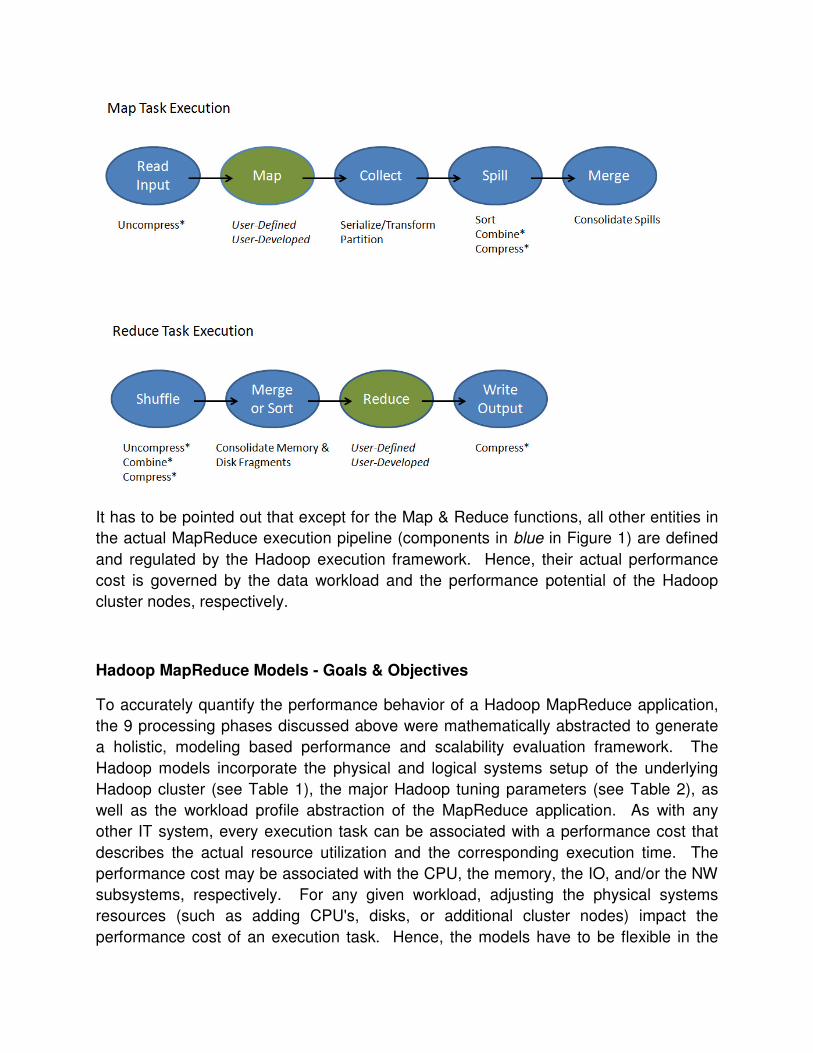
It has to be pointed out that except for the Map & Reduce functions, all other entities in

the actual MapReduce execution pipeline (components in blue in Figure 1) are defined

and regulated by the Hadoop execution framework. Hence, their actual performance

cost is governed by the data workload and the performance potential of the Hadoop

cluster nodes, respectively.

Hadoop MapReduce Models - Goals & Objectives

To accurately quantify the performance behavior of a Hadoop MapReduce application,

the 9 processing phases discussed above were mathematically abstracted to generate

a holistic, modeling based performance and scalability evaluation framework. The

Hadoop models incorporate the physical and logical systems setup of the underlying

Hadoop cluster (see Table 1), the major Hadoop tuning parameters (see Table 2), as

well as the workload profile abstraction of the MapReduce application. As with any

other IT system, every execution task can be associated with a performance cost that

describes the actual resource utilization and the corresponding execution time. The

performance cost may be associated with the CPU, the memory, the IO, and/or the NW

subsystems, respectively. For any given workload, adjusting the physical systems

resources (such as adding CPU's, disks, or additional cluster nodes) impact the

performance cost of an execution task. Hence, the models have to be flexible in the

sense that any changes to the physical cluster setup can be quantified via the models

(with high fidelity). The same statement holds true for the Hadoop and the Linux tuning

opportunities. In other words, adjusting the number of Map and/or Reduce task slots in

the model will change the execution behavior of the application and hence impact the

performance cost of the individual execution tasks [7]. As with the physical cluster

systems resource adjustments, the logical resource modifications have to result in

accurate performance predictions.

Map Tasks - Data Flow (Modeling) Highlights

As depicted in Figure 1, during the Map task read phase, the actual input split is loaded

from HDFS, if necessary uncompressed and the key-value pairs are generated and

passed as input to the user-defined and user-developed map function. If the

MapReduce job only entails map tasks (aka the number of reducers is set to 0), the spill

and merge phase will not occur and the map output will directly be transferred back into

HDFS. The map function produces output key-value pairs (records) that are stored in a

map-side memory buffer (labeled MemorySortSize in the model - see Table 2). This

output buffer is split in 2 parts. One part stores the actual bytes of the output data and

the other one holds 16 bytes of metadata per output. These 16 bytes include 12 bytes

for the key-value offset and 4 bytes for the indirect-sort index. When either of these 2

logical components fill-up to a certain threshold (determined in the model by

SortRecPercent), the spill process commences. The number of pairs and the size of

each spill file (the amount of data transferred to disk) depends on the width of each

record and the possible usage of a combiner and/or some form of data compression.

The objective of the merge phase is to consolidate all the spill files into a single output

file that is transferred into the local disk subsystem. It has to be pointed out that the

merge phase only happens if more than 1 spill file is generated. Based on the setup

(StreamsMergeFactor) and the actual workload conditions, several merge iterations

may occur. The StreamsMergeFactor model parameter governs the maximum number

of spill files that can be merged together into a single file. The first merge iteration is

distinct as Hadoop calculates the best possible number of spill files to merge so that all

the other (potential) merge iterations consolidate exactly StreamsMergeFactor files.

The last merge iteration is unique as well, as if the number of spills to be merged is >=

SpillsCombiner, the combiner is invoked again. The aggregate performance behavior

of the map tasks is governed by the actual workload, the systems setup, as well as the

performance potential of the CPU, memory, interconnect, and local IO subsystems,

respectively.

Reduce Tasks - Data Flow (Modeling) Highlights

During the shuffle phase, the execution framework fetches the applicable map output

partition from each mapper (labeled a map segment) and moves it to the reducer’s

node. In the case the map output is compressed, Hadoop will uncompress the data

(after the transfer) as part of the shuffling process. Depending on the actual segment

size, 2 different scenarios are possible at this stage. If the uncompressed segment size

is < 25% of (ShuffleHeapPercent*JavaHeapSpace - see Table 2) the map segments are

placed in the shuffle buffer. In scenarios where either the amount of data in the shuffle

buffer reaches (ShuffleHeapPercent*JavaHeapSpace) or the number of segments is >

MemoryMergeThr, the segments are consolidated and moved as a shuffle file to the

local disk subsystem. If the execution framework utilizes a combiner, the operation is

applied during the merge phase. If data compression is stipulated, the map segments

are compressed after the merge and prior to be written out to disk. If the uncompressed

segment size is >= 25% of (ShuffleHeapPercent*JavaHeapSpace), the map segments

are immediately moved into the local IO subsystem, forming a shuffle file on disk.

Depending on the setup and the workload at hand, both scenarios may create a set of

shuffle files in the local disk subsystem. If the number of on-disk shuffle files is >

(2*StreamsMergeFactor -1), a new merge thread is launched and StreamsMergeFactor

files are consolidated into a new and sorted shuffle file. If a combiner is used in the

execution framework, the combiner is not active during this disk merge phase. After

finalizing the shuffle phase, a set of merged and unmerged shuffle files may exist in the

local IO subsystem (as well as a set of map segments in memory). Next to the actual

workload conditions, the aggregate performance cost of the shuffle phase is impacted

by the cluster interconnect (data transfer), the performance of the memory and the CPU

subsystem (in-memory merge operations), as well as by the performance potential of

the local IO subsystem (on-disk merge operations).

After the entire map output data set has been moved to the reduce nodes, the merge

phase commences. During this phase, the map output data is consolidated into a single

stream that is passed as input into the reduce function for processing. Similar to the

map merge phase discussed above, the reduce merge phase may be processed in

multiple iterations. However, instead of compiling a single output file during the final

merge iteration, the actual data is moved directly to the reduce function. In the reduce

task, actual merging in this phase is considered a (potential) 3 step process. In step 1,

based on the setting of the ReduceMemPercent parameter, some map segments may

be marked for expulsion from the memory subsystem. This parameter governs the

amount of memory allowed to be used by the map segments prior to initiating the

reduce function. In scenarios where the number of shuffle files on disk is <

StreamsMergeFactor, the map segments marked for memory eviction are consolidated

into a single shuffle file on disk. Otherwise, the map segments that are marked for

expulsion will not be merged with the shuffle files on disk until step 2 and hence, step 1

does not happen. During step 2, any shuffle files residing in the local disk subsystem

go through an iterating merge process. It has to be pointed out that the shuffle files on

disk may be of varying sizes and that step 2 only happens if there are any actual shuffle

files stored on disk. Step 3 involves merging all data (in memory and on disk). This

process may complete in several iterations as well. The total performance cost of the

merge phase depends on the actual workload, the systems setup, and the performance

potential of the CPU, memory, and local IO subsystems, respectively.

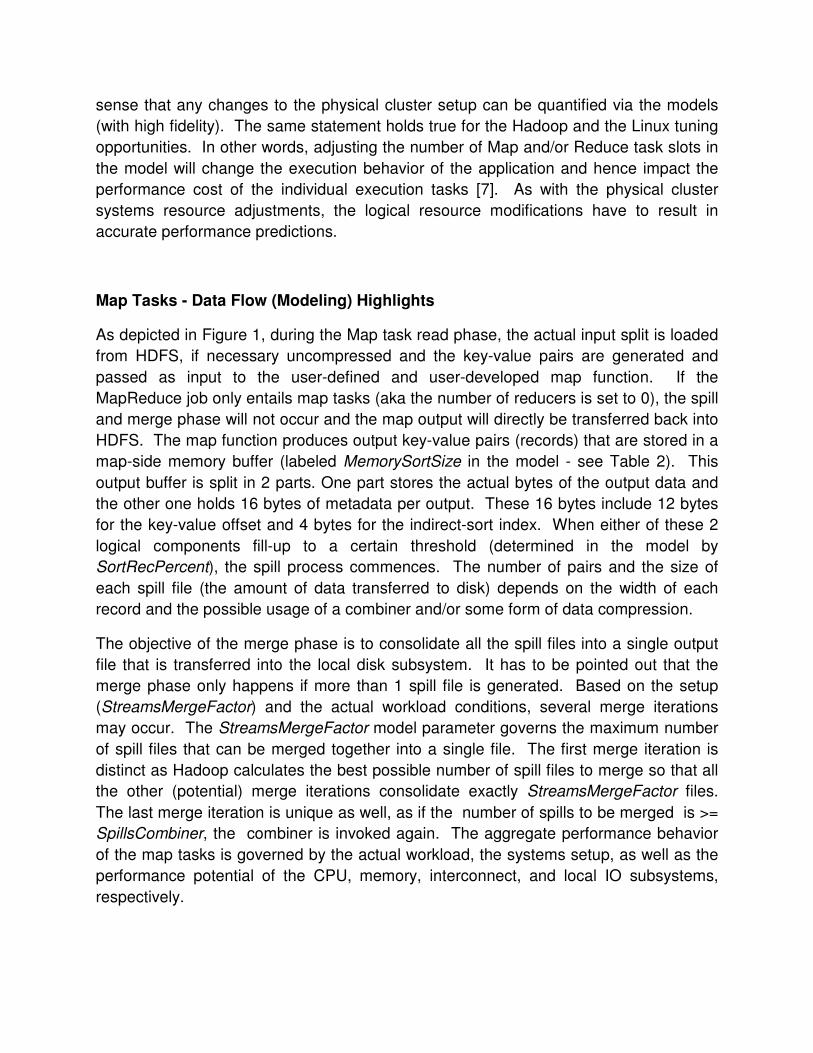
Table 1: Systems & Linux OS Parameters supported in the Models

CPUClockSpeed CPU Clock Speed (GHz)

NumCores Number of CPU's or CPU Cores

MemoryWidth Memory Interconnect Width (bytes)

MemCap Total Memory per Node (GB)

MemCycleTime Average Memory Cycle Time (ns)

NumLocalDisks Number of Local Disks per Node

AvgDiskLatency Average Local Disk Latency (ms)

AvgDiskSpeed Average Local Disk Throughput (MB/s)

ClusterNodes Number of Nodes in the Cluster

Interconnect GigE, 10GigE, IB, Custom

MTU Cluster Interconnect MTU (bytes)

HDFSBlockSize Configured HDFS Block Size (MB)

IOSched CFQ, deadline, noop

ReadAhead ReadAhead Size (in 512byte Blocks)

DiskType SSD, HD

Ultimately, the user-defined and user-developed reduce function is invoked,

processing the merged, intermediate data to compile the final output that is moved into

HDFS. It has to be pointed out that based on the shuffle and merge phase, the actual

input data into the reduce function may reside in both, the memory and the local disk

subsystems, respectively. As for the map tasks, the aggregate performance behavior of

the reduce tasks is determined by the actual workload, the systems setup, and the

performance potential of the CPU, memory, interconnect, and local IO subsystems,

respectively.

Model Profiles, Calibration & Validation

Further deciphering the (above discussed) execution of a MapReduce job discloses

rather specific execution functions and well-defined data processing phases.

Conceptually, only the map and the reduce functions are user-developed and hence

their execution is governed by user-defined and job specific actions. The execution of

all the other 7 processing phases are generic and only depend on the workload to be

processed and the performance potential and setup of the underlying Hadoop physical

and logical cluster resources, respectively. In other words, besides the map and the

reduce phase, all the other application processing cycles performance behavior is

controlled by the data being processed in that particular phase and the HW/SW

performance capacity of the cluster itself. To calibrate the Hadoop MapReduce models,

actual HW systems and workload profiles were established. The HW systems profiles

represent a detailed description of the individual physical systems components that

comprise the Hadoop cluster and disclose the performance potential (upper bound) of

the Hadoop execution framework (CPU, memory, Interconnect, local IO subsystem).

Due to protocol overhead, that performance potential can only be closely approached

by an actual application workload. The workload profiles detail the performance costs

of the individual execution phases and reflect the dynamics of the application

infrastructure. The workload profiles further quantify how much of the HW capacity is

being used and hence the HW and workload profiles can be used for capacity analysis

purposes. Table 1 outlines the major HW/SW parameters that are used as input into

the Hadoop MapReduce models.

Table 2: Major Hadoop Tuning Parameters supported in the Models

JavaHeapSpace mapred.child.java.opts

MaxMapTasks mapreduce.tasktracker.map.tasks.maximum

MaxReduceTasks mapreduce.tasktracker.reduce.tasks.maximum

NumMapTasksJob mapreduce.job.maps

MemorySortSize mapreduce.task.io.sort.mb

BufferSortLimit mapreduce.map.sort.spill.percent

SortRecPercent io.sort.record.percent

StreamsMergeFactor mapreduce.task.io.sort.factor

SpillsCombiner mapreduce.map.combine.minspills

NumReduceTasksJob mapreduce.job.reduces

MemoryMergeThr mapreduce.reduce.merge.inmem.threshold

ShuffleHeapPercent mapreduce.reduce.shuffle.input.buffer.percent

ShuffleMergePercent mapreduce.reduce.shuffle.merge.percent

ReduceMemPercent mapreduce.reduce.input.buffer.percent

UseCombine mapreduce.job.combine.class

CompressMapOut mapreduce.map.output.compress

CompressJobOut mapreduce.output.fileoutputformat.compress

CompressInput Flag - Input Compressed

InputDataSize Size of Input Split

While other Hadoop performance evaluation and quantification studies suggest the

usage of an application profiling tool [2],[3],[11], the argument made in this study is that

by solely profiling at the application layer, the level of detail necessary to conduct

comprehensive sensitivity studies via the Hadoop models is not sufficient. To illustrate,

any IO request at the application layer is potentially transformed at the Linux BIO layer,

the Linux IO scheduler, the device firmware, and the disk cache subsystem,

respectively. Further, the workload-dependent IO performance behavior is impacted by

some of the Linux specific logical resource parameters such as the setting of the read-

ahead value and/or the IO scheduler being used (see Table 1). To illustrate, the Linux

kernel tends to asynchronously read-ahead data from the disk subsystem if a sequential

access pattern is detected. Currently, the default Linux read-ahead block size equals to

128KBytes (can be adjusted via blockdev --setra). As Hadoop fetches data in a

synchronous loop, Hadoop cannot take advantage of OS' asynchronous read-ahead

potential past the 128KBytes unless the read-ahead size is adjusted on the cluster

nodes. Depending on the IO behavior of the MapReduce applications, it is rather

common to increase the read-ahead size in a Hadoop cluster environment.

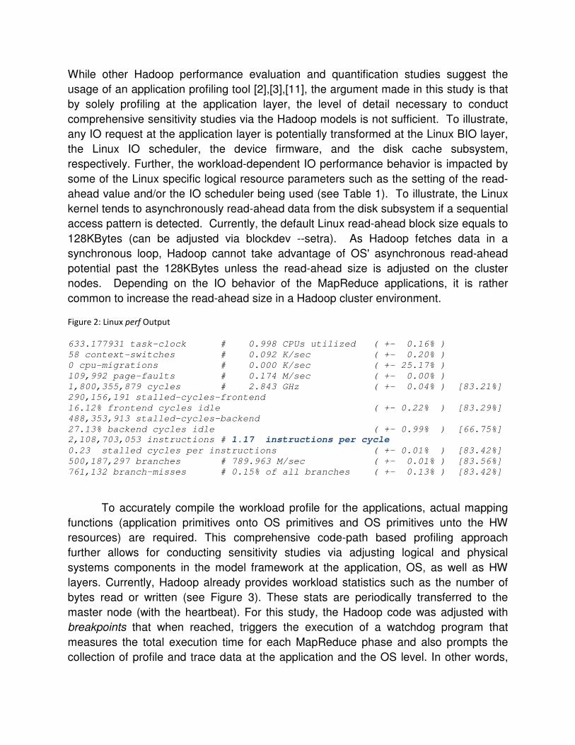
Figure 2: Linux perf Output

633.177931 task-clock # 0.998 CPUs utilized ( +- 0.16% )

58 context-switches # 0.092 K/sec ( +- 0.20% )

0 cpu-migrations # 0.000 K/sec ( +- 25.17% )

109,992 page-faults # 0.174 M/sec ( +- 0.00% )

1,800,355,879 cycles # 2.843 GHz ( +- 0.04% ) [83.21%]

290,156,191 stalled-cycles-frontend

16.12% frontend cycles idle ( +- 0.22% ) [83.29%]

488,353,913 stalled-cycles-backend

27.13% backend cycles idle ( +- 0.99% ) [66.75%]

2,108,703,053 instructions # 1.17 instructions per cycle

0.23 stalled cycles per instructions ( +- 0.01% ) [83.42%]

500,187,297 branches # 789.963 M/sec ( +- 0.01% ) [83.56%]

761,132 branch-misses # 0.15% of all branches ( +- 0.13% ) [83.42%]

To accurately compile the workload profile for the applications, actual mapping

functions (application primitives onto OS primitives and OS primitives unto the HW

resources) are required. This comprehensive code-path based profiling approach

further allows for conducting sensitivity studies via adjusting logical and physical

systems components in the model framework at the application, OS, as well as HW

layers. Currently, Hadoop already provides workload statistics such as the number of

bytes read or written (see Figure 3). These stats are periodically transferred to the

master node (with the heartbeat). For this study, the Hadoop code was adjusted with

breakpoints that when reached, triggers the execution of a watchdog program that

measures the total execution time for each MapReduce phase and also prompts the

collection of profile and trace data at the application and the OS level. In other words,

for the duration of each phase (see Figure 1), the task execution is profiled and traced

via the Linux tools strace, perf, blktrace and snapshots via lsof, iotop, ioprofile, and dstat

are taken. The breakpoints in the Hadoop code can individually be activated and

deactivated and as the actual trace and profile data is collected outside of the Hadoop

framework, the performance impact on the MapReduce execution behavior is

minimized.

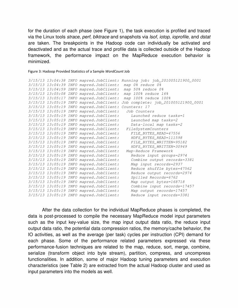
Figure 3: Hadoop Provided Statistics of a Sample WordCount Job

3/15/13 13:04:38 INFO mapred.JobClient: Running job: job_201005121900_0001

3/15/13 13:04:39 INFO mapred.JobClient: map 0% reduce 0%

3/15/13 13:04:59 INFO mapred.JobClient: map 50% reduce 0%

3/15/13 13:05:08 INFO mapred.JobClient: map 100% reduce 16%

3/15/13 13:05:17 INFO mapred.JobClient: map 100% reduce 100%

3/15/13 13:05:19 INFO mapred.JobClient: Job complete: job_201005121900_0001

3/15/13 13:05:19 INFO mapred.JobClient: Counters: 17

3/15/13 13:05:19 INFO mapred.JobClient: Job Counters

3/15/13 13:05:19 INFO mapred.JobClient: Launched reduce tasks=1

3/15/13 13:05:19 INFO mapred.JobClient: Launched map tasks=2

3/15/13 13:05:19 INFO mapred.JobClient: Data-local map tasks=2

3/15/13 13:05:19 INFO mapred.JobClient: FileSystemCounters

3/15/13 13:05:19 INFO mapred.JobClient: FILE_BYTES_READ=47556

3/15/13 13:05:19 INFO mapred.JobClient: HDFS_BYTES_READ=111598

3/15/13 13:05:19 INFO mapred.JobClient: FILE_BYTES_WRITTEN=95182

3/15/13 13:05:19 INFO mapred.JobClient: HDFS_BYTES_WRITTEN=30949

3/15/13 13:05:19 INFO mapred.JobClient: Map-Reduce Framework

3/15/13 13:05:19 INFO mapred.JobClient: Reduce input groups=2974

3/15/13 13:05:19 INFO mapred.JobClient: Combine output records=3381

3/15/13 13:05:19 INFO mapred.JobClient: Map input records=2937

3/15/13 13:05:19 INFO mapred.JobClient: Reduce shuffle bytes=47562

3/15/13 13:05:19 INFO mapred.JobClient: Reduce output records=2974

3/15/13 13:05:19 INFO mapred.JobClient: Spilled Records=6762

3/15/13 13:05:19 INFO mapred.JobClient: Map output bytes=168718

3/15/13 13:05:19 INFO mapred.JobClient: Combine input records=17457

3/15/13 13:05:19 INFO mapred.JobClient: Map output records=17457

3/15/13 13:05:19 INFO mapred.JobClient: Reduce input records=3381

After the data collection for the individual MapReduce phases is completed, the

data is post-processed to compile the necessary MapReduce model input parameters

such as the input key-value size, the map input output data ratio, the reduce input

output data ratio, the potential data compression ratios, the memory/cache behavior, the

IO activities, as well as the average (per task) cycles per instruction (CPI) demand for

each phase. Some of the performance related parameters expressed via these

performance-fusion techniques are related to the map, reduce, sort, merge, combine,

serialize (transform object into byte stream), partition, compress, and uncompress

functionalities. In addition, some of major Hadoop tuning parameters and execution

characteristics (see Table 2) are extracted from the actual Hadoop cluster and used as

input parameters into the models as well.

Hadoop Performance Evaluation and Results

For the modeling and sensitivity studies, 2 Hadoop cluster environments were used.

First, a 6-node Hadoop cluster that was configured in a 1 JobTracker/NameNode and 5

TaskTracker setup. All the nodes were configured with dual-socket quad-core Intel

Xeon 2.93GHz processors, 8GB (DDR3 ECC 1333MHz) of memory, and were equipped

with 4 1TB 7200RPM SATA drives each. Second, a 16-node Hadoop cluster, with 1

node used as the JobTracker, 1 node as the NameNode, and 14 nodes as

TaskTrackers, respectively. All the nodes in the larger Hadoop framework were

configured identically to the 6-node execution framework, except on the IO side. Each

node in the larger Hadoop setup was equipped with 6 1TB 7200RPM SATA drives. For

both Hadoop cluster setups, the cluster interconnect was configured as a switched GigE

network. Both clusters were powered by Ubuntu 12.04 (kernel 3.6) and CDH4 Hadoop.

For all the benchmarks, replication was set to 3. The actual Hadoop performance

evaluation study was executed in 6 distinct phases:

1. Establish the Model profiles (as discussed in this paper) for the 3 Hadoop

benchmarks TeraSort, K-Means, and WordCount on the 6-node Hadoop cluster.

All 3 benchmarks disclose different workload behaviors and hence reflect a good

mix of MapReduce challenges (see Figure 4). For these benchmark runs, the

default Java, Hadoop, and Linux kernel parameters were used (aka no tuning

was applied). In other words, the HDFS block size was 64MB, the Java Heap

space 200MB, the Linux read-ahead 256KB, and 2 Map and 2 Reduce slots were

used per node.

2. Use the established workload profiles in conjunction with the HW profiles to

calibrate and validate the Hadoop models. Execute the simulation and determine

the description error (delta empirical to model job execution time).

3. Use the developed Hadoop models to optimize/tune the actual workload based

on the physical and logical resources available in the 6-node Hadoop model. In

this stage, the methodology outlined in [10] was used to optimize/tune the

Hadoop environment via the models.

4. Apply the model-based tuning recommendations to the 6-node cluster. Rerun the

Hadoop benchmarks and establish the description error (delta tuned-empirical to

tuned-model job execution time).

5. Use the tuned-model baseline to conduct a scalability analysis, scaling the

workload input (increase the problem size) and mapping that new workload onto

a 16-node Hadoop cluster that is equipped with 6 instead of 4 SATA drives per

TaskTracker.

6. Execute the actual Hadoop benchmarks on the 16-node Hadoop cluster (with the

tuning and setup recommendations made via the model). Establish the

description error tuned-scaled-empirical to tuned-scaled-model job execution

time.

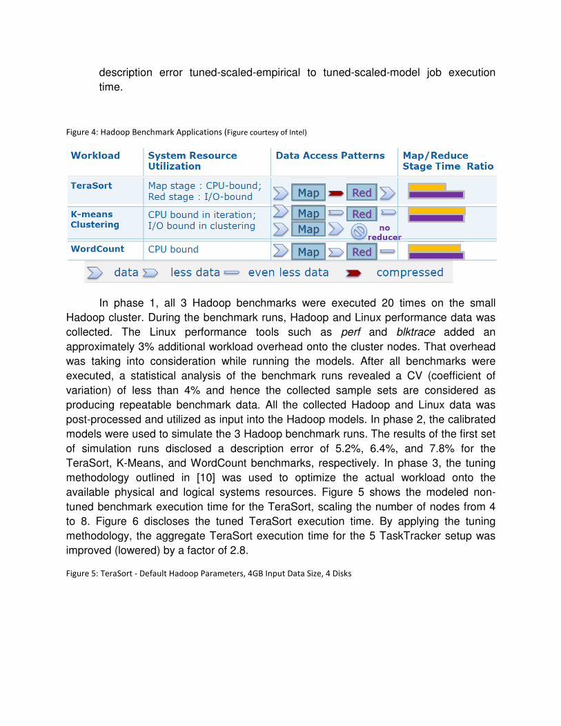
Figure 4: Hadoop Benchmark Applications (Figure courtesy of Intel)

In phase 1, all 3 Hadoop benchmarks were executed 20 times on the small

Hadoop cluster. During the benchmark runs, Hadoop and Linux performance data was

collected. The Linux performance tools such as perf and blktrace added an

approximately 3% additional workload overhead onto the cluster nodes. That overhead

was taking into consideration while running the models. After all benchmarks were

executed, a statistical analysis of the benchmark runs revealed a CV (coefficient of

variation) of less than 4% and hence the collected sample sets are considered as

producing repeatable benchmark data. All the collected Hadoop and Linux data was

post-processed and utilized as input into the Hadoop models. In phase 2, the calibrated

models were used to simulate the 3 Hadoop benchmark runs. The results of the first set

of simulation runs disclosed a description error of 5.2%, 6.4%, and 7.8% for the

TeraSort, K-Means, and WordCount benchmarks, respectively. In phase 3, the tuning

methodology outlined in [10] was used to optimize the actual workload onto the

available physical and logical systems resources. Figure 5 shows the modeled non-

tuned benchmark execution time for the TeraSort, scaling the number of nodes from 4

to 8. Figure 6 discloses the tuned TeraSort execution time. By applying the tuning

methodology, the aggregate TeraSort execution time for the 5 TaskTracker setup was

improved (lowered) by a factor of 2.8.

Figure 5: TeraSort - Default Hadoop Parameters, 4GB Input Data Size, 4 Disks

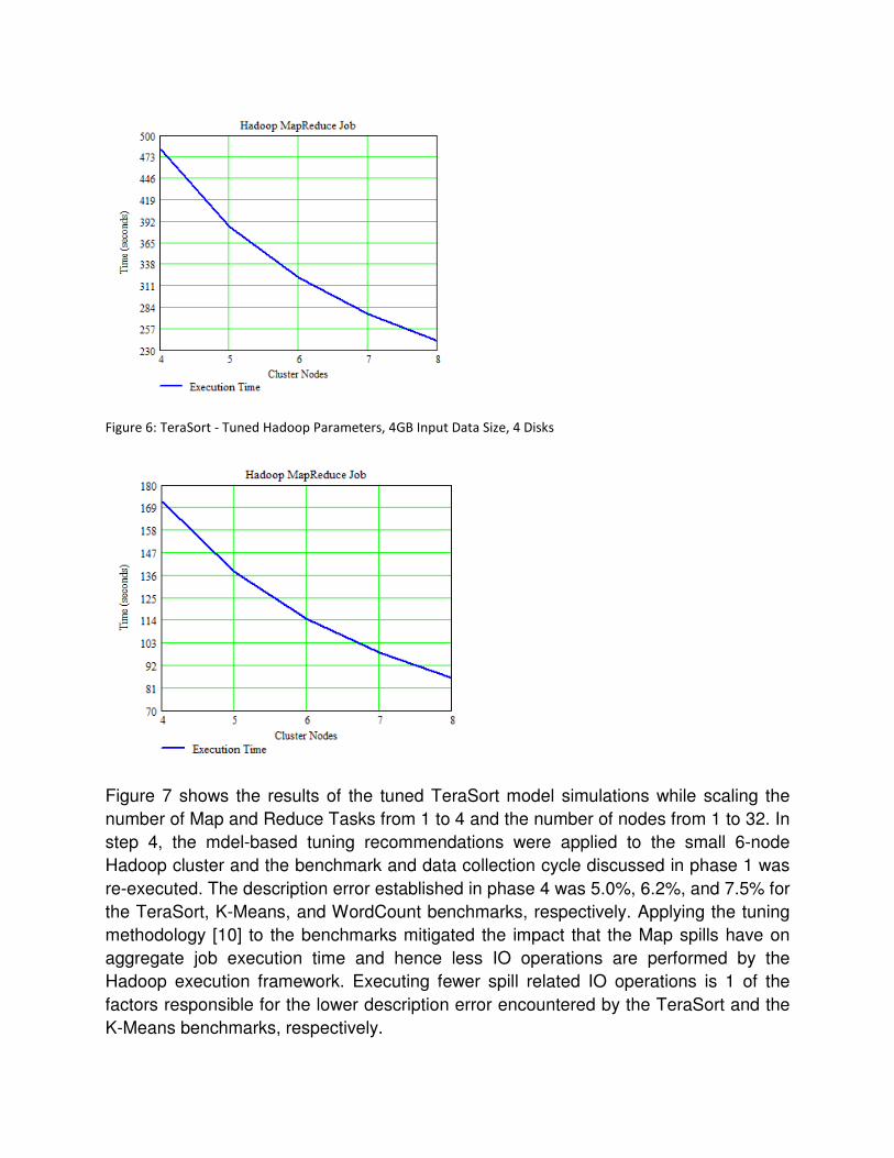
Figure 6: TeraSort - Tuned Hadoop Parameters, 4GB Input Data Size, 4 Disks

Figure 7 shows the results of the tuned TeraSort model simulations while scaling the

number of Map and Reduce Tasks from 1 to 4 and the number of nodes from 1 to 32. In

step 4, the mdel-based tuning recommendations were applied to the small 6-node

Hadoop cluster and the benchmark and data collection cycle discussed in phase 1 was

re-executed. The description error established in phase 4 was 5.0%, 6.2%, and 7.5% for

the TeraSort, K-Means, and WordCount benchmarks, respectively. Applying the tuning

methodology [10] to the benchmarks mitigated the impact that the Map spills have on

aggregate job execution time and hence less IO operations are performed by the

Hadoop execution framework. Executing fewer spill related IO operations is 1 of the

factors responsible for the lower description error encountered by the TeraSort and the

K-Means benchmarks, respectively.

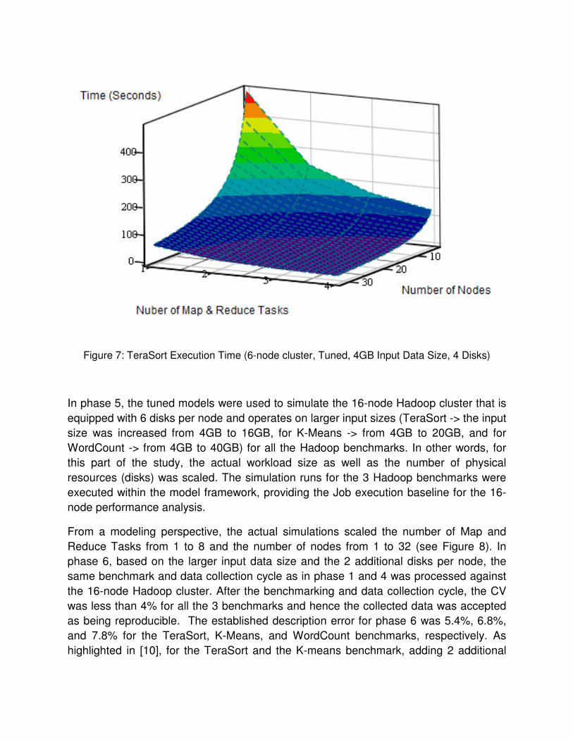
Figure 7: TeraSort Execution Time (6-node cluster, Tuned, 4GB Input Data Size, 4 Disks)

In phase 5, the tuned models were used to simulate the 16-node Hadoop cluster that is

equipped with 6 disks per node and operates on larger input sizes (TeraSort -> the input

size was increased from 4GB to 16GB, for K-Means -> from 4GB to 20GB, and for

WordCount -> from 4GB to 40GB) for all the Hadoop benchmarks. In other words, for

this part of the study, the actual workload size as well as the number of physical

resources (disks) was scaled. The simulation runs for the 3 Hadoop benchmarks were

executed within the model framework, providing the Job execution baseline for the 16-

node performance analysis.

From a modeling perspective, the actual simulations scaled the number of Map and

Reduce Tasks from 1 to 8 and the number of nodes from 1 to 32 (see Figure 8). In

phase 6, based on the larger input data size and the 2 additional disks per node, the

same benchmark and data collection cycle as in phase 1 and 4 was processed against

the 16-node Hadoop cluster. After the benchmarking and data collection cycle, the CV

was less than 4% for all the 3 benchmarks and hence the collected data was accepted

as being reproducible. The established description error for phase 6 was 5.4%, 6.8%,

and 7.8% for the TeraSort, K-Means, and WordCount benchmarks, respectively. As

highlighted in [10], for the TeraSort and the K-means benchmark, adding 2 additional

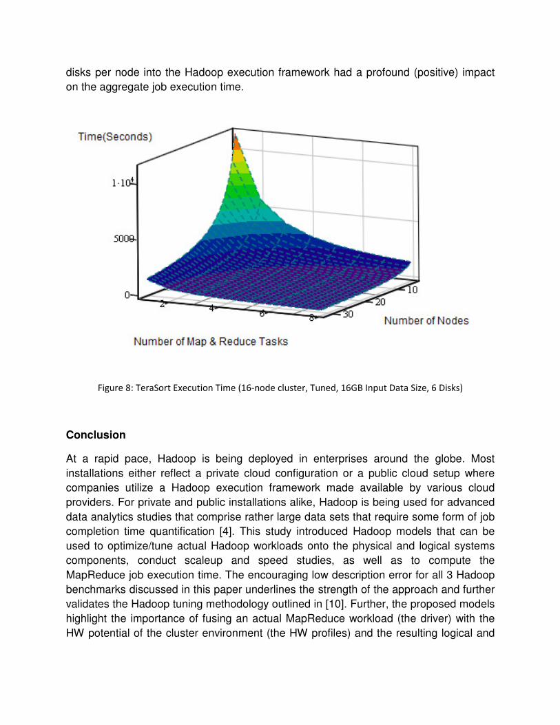
disks per node into the Hadoop execution framework had a profound (positive) impact

on the aggregate job execution time.

Figure 8: TeraSort Execution Time (16-node cluster, Tuned, 16GB Input Data Size, 6 Disks)

Conclusion

At a rapid pace, Hadoop is being deployed in enterprises around the globe. Most

installations either reflect a private cloud configuration or a public cloud setup where

companies utilize a Hadoop execution framework made available by various cloud

providers. For private and public installations alike, Hadoop is being used for advanced

data analytics studies that comprise rather large data sets that require some form of job

completion time quantification [4]. This study introduced Hadoop models that can be

used to optimize/tune actual Hadoop workloads onto the physical and logical systems

components, conduct scaleup and speed studies, as well as to compute the

MapReduce job execution time. The encouraging low description error for all 3 Hadoop

benchmarks discussed in this paper underlines the strength of the approach and further

validates the Hadoop tuning methodology outlined in [10]. Further, the proposed models

highlight the importance of fusing an actual MapReduce workload (the driver) with the

HW potential of the cluster environment (the HW profiles) and the resulting logical and

physical resource allocation (the code-path based workload profiles) while conducting a

performance evaluation.

Acknowledgments

Countless scientists and engineers are currently working on improving and

optimizing the execution framework necessary to conduct Big Data studies. From

developing new tools for Big Data to improving Hadoop and machine learning

algorithms, countless hours are spent on identifying actual execution frameworks that

allow customers to receive answers as quickly as possible. While there are countless

other scientists involved in this effort, the author of this report would like to thank Dr.

Biem (IBM Watson - Big Data Research) and Dr. Herodotou (Duke University) for

spearheading some of these efforts by providing new ideas and methodologies to

address the discussed Big Data issues head-on.

References

1. H. Herodotou, "Hadoop Performance Models", Technical Report, CS-2011-05, Duke University, February 2011

2. H. Lim, H. Herodotou, and S. Babu. "Stubby: A Transformation-based Optimizer

for MapReduce Workflows.", In Proc. of the 38th Intl. Conf. on Very Large Data Bases (VLDB '12), August 2012.

3. Andy Konwinski, Matei Zaharia, Randy Katz, Ion Stoica, "X-Tracing Hadoop", CS

division UC Berkeley, 2012

4. Alain Biem and Nathan Caswell, "A value network model for strategic analysis", 41st Hawaii International Conference on System Sciences, 2008

5. Biem, A. ; Feng, H. ; Riabov, A.V. ; Turaga, D.S., "Real-time analysis and

management of big time-series data", IBM Journal of Research and Development, 2013

6. W. Lang and J. M. Patel. "Energy Management for MapReduce Clusters". In

Proceedings of the VLDB Endowment, 2010

7. J. Leverich and C. Kozyrakis. "On the Energy (In)efficiency of Hadoop Clusters". SIGOPS Operating Systems Review, 2010

8. D. Meisner and T. F. Wenisch. "Stochastic Queuing Simulation for Data Center

Workloads". In Proceedings of the Workshop on Exascale, Evaluation and Research Techniques, 2010

9. M. Zaharia, A. Konwinski, A. D. Joseph, R. Katz, and I. Stoica. "Improving MapReduce Performance in Heterogeneous Environments". In Proceedings of the USENIX Conference on Operating Systems Design and Implementation, 2008

10. Heger, D., "Hadoop Performance Tuning - A Pragmatic & Iterative Approach",

CMG Journal, 2013

11. "BTrace, A Dynamic Instrumentation Tool for Java", kenai.com/projects/btrace

12. "Apache Hadoop", http://hadoop.apache.org/

13. "HDFS", http://hadoop.apache.org/hdfs/