Working Paper Series - Federal Reserve Bank of Richmond · mobile case, inter-industry local...

Working Paper Series

This paper can be downloaded without charge from: http://www.richmondfed.org/publications/

Competitors, Complementors, Parents and Places:Explaining Regional Agglomerationin the U.S. Auto Industry

Luıs CabralNew York University and CEPR

Zhu WangFederal Reserve Bank of Richmond

Daniel Yi XuDuke University and NBER

Working Paper No. 13-04R

This draft: January 2018

Abstract. Taking the early U.S. automobile industry as an example, we evaluate four competing hy-potheses on regional industry agglomeration: intra-industry local externalities, inter-industry localexternalities, employee spinouts, and location fixed effects. Our findings suggest that in the auto-mobile case, inter-industry local externalities (particularly from the carriage and wagon industry)and employee spinouts (particularly due to the high spinout rate in Detroit) play important roles.The presence of other firms in the same industry has a negligible or negative effect. Finally, localinputs account for some agglomeration in the short run, but the effects are much more profound inthe long run.

JEL classification: L26; L6; R1Keywords: Local externalities; Spinouts; Location advantages; Industry agglomeration

Forthcoming, Review of Economic Dynamics. Cabral: Paganelli-Bull Professor of Economics and InternationalBusiness, Stern School of Business, New York University; IME and PS-PS (IESE) Research Fellow; and ResearchFellow, CEPR (London); [email protected]. Wang: Research Department, Federal Reserve Bank of Richmond;[email protected]. Xu: Department of Economics, Duke University; [email protected].

We thank the editor and two anonymous referees for their valuable comments and suggestions. We also thank EdGlaeser, Tom Holmes, Hugo Hopenhayn, Boyan Jovanovic, Bob Lucas, Esteban Rossi-Hansberg and participants atvarious conferences and seminars for helpful comments; and Christian Hung, Roisin McCord and Erica Paulos forexcellent research assistance. The views expressed herein are solely those of the authors and do not necessarilyreflect the views of the Federal Reserve Bank of Richmond or the Federal Reserve System.

1. Introduction

Why do some industries concentrate in certain geographic locations? Ever since Marshall’s (1890)seminal work, an intense debate has developed among economists regarding agglomeration external-ities. Marshall himself pointed to positive externalities from specialization: regions with specializedproduction structures tend to be more innovative in their specific industries. In particular, Marshallpointed to the importance of knowledge spillovers: each firm learns from neighboring firms in thesame industry.

Employees from different firms in an industry exchange ideas about new products andnew ways to produce goods: the denser the concentration of employees in a commonindustry in a given location, the greater the opportunity to exchange ideas that lead tokey innovations.

Marshall’s work was later extended by the work of many authors, including Arrow (1962) and Romer(1986).1 (Knowledge spillovers are sometimes referred to as MAR spillovers.) We should note that,in addition to knowledge spillovers, Marshall also considered other types of externalities, includinginput sharing and labor pooling. However, as Ellison, Glaeser and Kerr (2010) argue, all of these“predict that firms will co-locate with other firms in the same industry.” Accordingly, we refer toMarshallian externalities as economic effects that lead firms to locate close to other firms of thesame industry: intra-industry externalities.2

In contrast to Marshallian externalities, other authors, most notably Jacobs (1969), proposed analternative agglomeration thesis, the idea that knowledge spills across different industries, causingdiversified production structures to be more innovative. For example, Jacobs (1969) argues thatthe growth of Detroit’s automobile industry may owe a great deal to the prior growth of Detroit’sshipbuilding industry.3 We refer to these externalities as inter-industry externalities (as opposed tointra-industry, or Marshallian, externalities).4

A different perspective on agglomeration is provided by the work of Klepper (2007), who focuseson the role of employee spinouts. He argues that

The agglomeration of the automobile industry around Detroit, Michigan is explained[by] disagreements [that] lead employees of incumbent firms to found spinoffs in thesame industry.5

The effect of spinouts on agglomeration is related to Marshallian externalities in the sense that thenumber of firms in a given industry is subject to self-reinforcing dynamics: the more industry ifirms are located at location j, the more likely new industry i firms will be located at location j.However, according to Klepper, the mechanism for these self-reinforcing dynamics is quite differentfrom Marshallian externalities; it results from organizational reproduction (that is, a “heredity”effect).

Finally, the work of Ellison and Glaeser (1997, 1999) suggests that much of the agglomerationobserved in U.S. manufacturing may be due simply to the relative advantage of certain locations,

1. See also Krugman (1991), Glaeser et al (1992) and Henderson et al (1995).2. It may be argued that we are taking a very narrow view of Marshallian externalities by restricting to other

firms within the same industry. In fact, we will next consider the possibility of externalities across relatedindustries. Our goal is to present an account of factors affecting industry agglomerations that is as detailed aspossible. For this reason, we believe it is helpful to make this distinction.

3. See also Jackson (1988).4. These externalities are sometimes referred to as co-agglomeration externalities. Some authors (e.g., Ellison,

Glaeser and Kerr, 2010) refer to agglomeration and co-agglomeration externalities as Marshallianexternalities. However, we believe the distinction between the two to be relevant. In fact, it corresponds to acentral piece of our theoretical and empirical exercise.

5. Buenstorf and Klepper (2009) paint a similar picture for the tire industry. Note that, while Klepper (2007)uses the term “spinoffs,” other authors including ourselves use the term “spinouts” (leaving the former termto designate the divestment of a firm’s unit).

1

such as the availability of natural resources. For example, the wine industry is located in California,not Kansas, largely due to California’s favorable weather.6

In this paper, we construct a detailed dataset of the evolution of the U.S. auto industry and runa “horse race” between alternative views of agglomeration: (a) intra-industry spillovers (“competi-tors,” as in the work of Marshall et al); (b) inter-industry spillovers (“complementors,” as in thework of Jacobs et al); (c) family network, or spinout, effects (“parents,” as in the work of Klepperet al); (d) location fixed effects (“places,” as in the work of Ellison and Glaeser).7

We first identify six historically important auto production centers from the data: New YorkCity, Chicago, Indianapolis, Detroit, Rochester, and St. Louis. This raises the important question:Why did these six locations rather than other places become prominent auto production centers?The data also shows that the relative importance of Detroit as a production center increased steadilysince the beginning of the 20th century. The auto industry eventually became highly concentratedin Detroit. Why?

Our analysis provides answers to the above questions and also refines the existing explanationsof industry agglomeration. First, in contrast to Marshall’s (1890) hypothesis, we find that theproximate presence of firms from the (narrowly defined) same industry (that is, the presence ofcompetitors) has a negligible or even negative effect on firm performance; we interpret this result asimplying that the negative competition externality outweighs Marshallian positive spillovers.

Second, regarding the ideas of Jacobs (1969) and others, we find evidence for strong positive inter-industry spillovers. However, as opposed to Jacobs (1969), the spillovers we find operate through thecarriage and wagon industry rather than the shipbuilding industry. To the extent that the carriageand wagon industry preceded and was supplanted by the auto industry, the agglomeration effectsthat Marshall (1890) pointed out to appear valid but need to be interpreted in a broader context.8

Third, consistent with Klepper (2007), our findings show that spinouts play an important roleon regional agglomeration, which contributed to the increased concentration in Detroit. However,we find that the performance of spinouts is heavily affected by local family members but not bydistant ones, which suggests that spinouts may actually benefit from intra-family local spilloversrather than the heredity effect. This finding helps to bridge the gap between Klepper (2007) andMarshall (1890).

Finally, consistent with the work of Ellison and Glaeser (1997, 1999), we find significant locationspecific effects, particularly in the long run: the search for locally available inputs led founders ofauto companies to Detroit; moreover, many of them were previously associated with local carriageand wagon companies, the location of which was in turn largely determined by the availability of localinputs. (To the best of our knowledge, we are the first to make this distinction, both conceptuallyand quantitatively.)

When discussing the evolution of the U.S. auto industry, a reference to the industry’s shakeout isinevitable. The industry started in the 1890s and the number of car producers reached more than 200around 1910. However, the number of firms declined since the mid-1910s (in spite of the considerableexpansion of industry output). Only 40 firms survived by the mid-1920s, and merely 8 made it into1940s.9 While the shakeout in terms of firm numbers is a phenomenon of unquestionable interest,it is largely independent of the central issue we study: industry agglomeration around Detroit and

6. Ellison and Glaeser (1997, 1999) also consider the possibility of “spurious” agglomeration due tonon-economic motives.

7. Other authors, most notably Klepper (2007), have also looked at the evolution of the U.S. auto industry. Inaddition to data on entries, exits and spinouts, we also obtained data on related industries and on the mostsignificant inputs to the auto industry. (To the best of our knowledge, ours is the first paper to work withdata of this nature.) Moreover, unlike Klepper (2007), who only examines the evolution of Detroit as aproduction center, we identify multiple production centers and look at the entire geographic distribution ofthe U.S. auto industry.

8. The positive spillovers from carriage and wagon (the precedent industry) to auto (the new industry) isnatural given that early automobiles were constructed in a very similar fashion to carriages, sharing identicalparts and mechanics. This is consistent with Klepper and Simons (2000), who find that the U.S. televisionreceiver industry was dominated by firms who had experiences producing radios prior to TVs.

9. As shown by Gort and Klepper (1982), this shakeout pattern is commonly observed in many industries, notjust automobile.

2

other clusters. As Figure 1 shows, well before the industry shakeout took place, agglomerationaround the six production centers — with Detroit being the largest one — had already emerged.Accordingly, our analysis focuses on the industry’s pre-shakeout stage, which also avoids concerns ofsurvivor bias in explaining industry agglomeration (that is, the idea that a few Detroit-based firmssurvived the shakeout, so that Detroit became effectively the dominant production center).

Our quantitative exercise begins with a series of reduced-form regressions explaining firm entryand survival. Based on these findings, we then construct a dynamic structural model and calibrateits stationary equilibrium to data from before the shakeout. Having calibrated the model, we conducta series of counterfactual simulations where a selected feature of the model (e.g., spinouts) is shutoff. We measure that feature’s contribution to agglomeration by the corresponding drop in modelgoodness of fit (both in absolute terms and as a fraction of the model’s total explained variation).Finally, by considering the endogeneity of carriage and wagon (C&W) firm location, we distinguishbetween short-term and long-term effects.

As mentioned earlier, we find the net contribution of competitors to be negative (that is, ag-glomeration takes place not because but in spite of the effect of local competitors). We also findthat the relative contribution of the remaining three channels — complementors, parents and places— depends on the time frame. In the short-run — that is, given location decisions in the C&Windustry — complementors and spinouts come out ahead in the “horse race.” In the long-run —that is, considering the endogeneity of C&W location decisions — location fixed effects, particularlydue to local input resources, come out ahead (again, together with spinouts).

Specifically, taking C&W locations as given we estimate that inter-industry spillovers contribute45.89% to explain total agglomeration; local input resources, 23.03%; and spinouts, 59.72%; allleading to a sum total greater than 100%, to compensate for the dispersion effect of local competi-tors. Taking explicit account of C&W location decisions, we estimate that inter-industry spilloverscontribute 9.78%; local input resources, 52.88%; and spinouts, 79.71%. In other words, much of theeffect of related industries is transferred to local input resources once we consider endogenous C&Wlocation decisions.

Finally, we note that almost the entirety of the effect of spinouts stems from allowing for a Detroit-specific spinout rate. This is consistent with the work of Marx, Strumsky and Fleming (2009), whostress the role of Michigan Statute 445.761 (of 1905) which prohibits non-compete agreements (andthus facilitates spinouts). This suggests that it’s not spinouts per se that account for agglomerationin the auto industry but rather the difference in spinout rates across regions, differences which inturn stem from location-specific effects (regulations in this case). In this sense, our findings can beinterpreted as implying that location-specific effects — including local inputs and location-specificspinout rates — accounted for the lion’s share of the auto industry agglomeration, both in the shortrun and in the long run.

Ours is not the first attempt at estimating the relative contribution of alternative agglomerationtheories. Ellison, Glaeser and Kerr (2010) “exploit patterns of industry coagglomeration to measurethe relative importance of different theories of industry agglomeration.” In particular, they areinterested in teasing out the relative importance of the three Marshallian channels: movementof goods, movement of people and movement of ideas.10 Our agglomeration accounting exercisecomplements theirs: we do not focus on the different channels proposed by Marshall;11 by contrast,we pay close attention to the distinction between intra and inter-industry spillovers. Our findingssuggest that the theories of Marshall (1890), Jacobs (1969), and Klepper (2007) are all relevant, butthey need to be interpreted in the correct context.

10. Summarizing Marshall’s points, Ellison, Glaeser and Kerr (2010) write: “First, he argued that firms willlocate near suppliers or customers to save shipping costs. Second, he developed a theory of labor marketpooling to explain clustering. Finally, he began the theory of intellectual spillovers by arguing that inagglomerations, ‘the mysteries of the trade become no mystery, but are, as it were, in the air.’ ”

11. As Ellison, Glaeser and Kerr (2010) rightly point out, “each Marshallian theory predicts that the same thingwill happen for similar reasons: plants will locate near other plants in the same industry because there is abenefit to locating near plants that share some characteristic.” Their results “support the importance of allthree Marshallian theories and the importance of shared natural advantages.”

3

Our paper is also related to recent work by Bloom et al (2013). They find that firm performanceis affected by two countervailing agglomeration effects: a positive effect from knowledge spillovers;and a negative business-stealing effect from product market rivalry. Our analysis is consistent withthis distinction. Specifically, we estimate that, when defining agglomeration effects narrowly, thecompetition effect dominates; whereas, when defining agglomeration effects broadly, the knowledgespillover effect dominates.

The rest of the paper is structured as follows. In Section 2, we briefly describe the background ofthe U.S. auto industry. Next, in Section 3 we run a series of reduced-form regressions that test therelative merit of various theories of industry agglomeration. The results motivate Section 4, wherewe develop and calibrate a dynamic structural model and run a series of counterfactual simulationsthat allow us to quantify the relative contribution of each agglomeration factor. Section 5 concludesthe paper.

2. The U.S. automobile industry

The U.S. auto industry went through tremendous development in its first 75 years, evolving froma small and fragmented infant industry into a gigantic, consolidated triopoly. During this process,the industry output continued to expand, but the number of firms initially rose and later fell: inits peak years around 1910, there were more than 200 producers, but only 8 survived in the 1940s.This is a common life-cycle pattern observed in many industries, termed as “industry shakeout” inthe literature.

In the meantime, the auto industry showed substantial changes in geographic concentration.Based on the data, we identified six historically important auto production centers: St. Louis,Chicago, Indianapolis, Detroit, Rochester, and New York City.12 Figure 1 presents the evolutionof U.S. auto production measured by each location’s share of the total number of firms from 1895to 1942. As can be seen, New York City and Chicago were the most important centers in the late1890s. Soon after, Detroit and other centers caught up. In 1905, 25% of all active firms were locatedin Detroit, 15% in New York City, 10% in Chicago, 8% in Indianapolis, 7% in Rochester, 2% in St.Louis, and the remaining 32% scattered across the country. In the years that followed, Detroit’sshare continued to increase.

As mentioned earlier, an important fraction of the industry entrants originated in other existingindustry firms: a spinout. We will refer to the firm originating the spinout as the “parent” and thespinout firm as a “child.” Sometimes, the “child” itself becomes a parent by originating a spinout.Together, spinouts give rise to “families” of auto firms, that is, groups of firms linked together byspinout relationships.

We identified a total of 53 spinout families over the history of the auto industry. The threelargest families were GM/Buick, Ford and Oldsmobile, all located in Detroit, each generating 12–17spinouts.13 As an example, Figure 2 displays the GM/Buick family tree. As can be seen, it’s afamily with three generations: for example, a former GM employee founded Chevrolet, from whichin turn Gardner and Monroe spun out.

Figure 3 plots the evolution of the number of spinout families and of family size. Early on,there were very few spinouts. For example, in 1900 only one spinout family existed (which hadtwo members including the parent), out of a total of 57 firms in the industry. In the followingtwo decades, the period of greatest industry turbulence (that is, highest entry and exit rates), thenumber of families was somewhere between 10 and 15, whereas average family size was somewherebetween 3 and 4. By 1920, 41 out of a total of 136 firms belonged to spinout families. Most spinouts

12. Lacking good data on firm size, we instead use the number of firms as a measure of regional agglomeration. Acity is counted as an auto production center city if it had at least five auto producers in 1910 (the peak yearof the auto industry in terms of firm numbers). We then define the region within 100 miles of the center cityas the production center, named after the center city (we tried different radiuses ranging from 25 miles to 150miles for the center definition, and the 100 mile radius appears to provide the overall best fit for the data).

13. Klepper (2007) constructed family trees for GM/Buick, Ford, Oldsmobile and Cadillac. The family membersthat he identified are largely consistent with ours.

4

Figure 1Geographical distribution of U.S. auto producers

0

50

100

1900 1910 1920 1930 1940

Percentage of U.S. producers

Year

Others

New York City

Rochester

Detroit

Indianapolis

Chicago

St Louis

Figure 2GM/Buick’s family tree

GM/Buick (1903–)

Welch-Detroit (1909–1909)

Lorraine (1919–1921)

Little (1911–1913)

Lincoln (1920–1922)

Daniels (1915–1923)

Chrysler (1924–)

Farmack (1915–1916)

Durant (1921–1931)

Nash (1917–1954)

Chevrolet (1911–1916)

Drexel (1917–1917)

DeVaux (1931–1933)

Lafeyette (1920–1924)

Monroe (1914–1920)

Gardner (1920–1931)

located near their parents. For example, 76% of the spinouts in the top three families stayed inDetroit.

Although our analysis focuses on the auto industry, there are related industries which play animportant role in explaining entry and exit patterns by auto firms. Prominent among these is thecarriage and wagon (C&W) industry. The left panel of Figure 4 plots the level of activity in theauto industry (measured by the number of firms in 1910, the peak year of the auto industry interms of firm numbers) against activity level in the C&W industry (measured by C&W employmentlevel in 1905).14 As can be seen, there is a clear positive correlation between the two. Obviously,at this stage there is little more to be said other than the fact that there is a correlation. Belowwe explore this relation in greater detail, and the results suggest that location patterns of auto

14. Given that only state-level data are available for C&W industry employment, we combine New York City andRochester together as New York in the figure. We also add up all other non-center states in the “other” group.

5

Figure 3Family size distribution of U.S. auto producers (1900–1925)

0

5

10

15

20

1900 1905 1910 1915 1920 1925

No. families (left) Average family size (right)

Year

1

2

3

4

5

Figure 4Location-level variables

0

20

40

60

80

0 5000 10000 15000 20000 25000

Number of auto producers 1910

1905 C&Wemployment

•

••

•

•

•

St Louis

Chicago

Indianapolis

Detroit

New York

Other

0

20

40

60

80

0 60 120 180 240

Number of auto producers 1910

1905inputs

•

••

•

•

•

StLouis

Chicago

Indianapolis

Detroit

NewYork

Other

firms (the new industry) were indeed influenced by location patterns of C&W firms (the precedentindustry). Similarly, we also examine the influence of the shipbuilding industry, which turns out tobe quite insignificant.

Why is the C&W industry important in studying the auto industry? Anecdotal evidence suggeststhat many auto firms were founded by experienced C&W veterans. One of the prominent figuresis William C. Durant, the founder of GM. Before entering the auto industry, he was running theDurant-Dort Carriage Company, based in Flint, Michigan, which was the largest manufacturer ofhorse-drawn vehicles in the nation at the time. Therefore, it is natural to think that the presenceof the C&W industry may have fostered the agglomeration of the new auto industry by providingthe human capital that the latter needed.

Aside from this channel, however, it is likely that other factors could also have contributed to theco-agglomeration of C&W and auto firms. For example, at the time both industries relied heavilyon common inputs, such as iron and lumber.15 The right panel of Figure 4 plots the concentrationof the auto industry against the index of local auto-related input resources.16 There is also a clearpositive correlation. In the following analysis, we will try to tease out various effects, and show

15. According to Census of the U.S. Manufactures 1905 and Leontief (1951), iron and steel, lumber and timber,brass and copper, and rubber were top inputs for both industries at the time.

16. The index of local auto-related input resources is constructed using historical data and the input-outputmatrix created by Leontief for the U.S. economy in 1919. See Section 3 for more details.

6

that the C&W industry and local inputs both affected the auto industry agglomeration but throughdifferent channels.

It is worth noting that the geographic concentration pattern of the U.S. auto industry hadformed well before the shakeout started around the mid-1910s. Our following analysis, therefore,will largely focus on the pre-shakeout stage of industry development. According to the classic theoryof Jovanovic and MacDonald (1994), new industries evolve over two stages: A new product leadsto the creation of a new industry, which in a first stage reaches a stationary equilibrium. In asecond stage, a major innovation (e.g., the introduction of assembly-line production into the autoindustry during the mid-1910s) leads to a survival race where firms unable to adopt the innovationare shaken out of the industry.17 While many forces that we identified with our reduced-form entryand exit regressions are relevant for both pre- and post-shakeout periods, our structural calibrationand agglomeration accounting exercises will focus on the pre-shakeout period, leaving the study ofindustry shakeout aside. As mentioned earlier, by doing so we also avoid concerns of survivor biasin explaining industry agglomeration.

To the extent that shakeout and geographic agglomeration are both commonly seen in manyindustries’ life cycles, the approach that we develop in this paper could potentially apply to otherindustries besides automobile. Our analysis points to the importance of distinguishing pre- and post-shakeout stages while conducting the agglomeration accounting exercise, so that the contribution ofeach agglomeration factor can be quantified in a clearly-defined industry development context.

3. Reduced-form regression analysis

In this section we present a series of reduced-form regressions that provide tests of various theoriesof industry agglomeration. Marshallian theories imply that a firm’s benefit from locating in regioni is increasing in the number of other firms located in region i. Everything else constant, we wouldexpect this to be reflected in entry rates and exit rates: entry rates are increasing in the number offirms, whereas exit rates are decreasing in the number of firms in region i.

Regarding co-agglomeration economies, our tests are based on data regarding the importance ofrelated industries, including the carriage and wagon industry and the shipbuilding industry. Thetheory prediction is that the presence of related industries improves a firm’s prospects, most likelythrough the human capital channel. We thus expect entry (respectively, exit) rates to be increasing(respectively, decreasing) in the employment size of related industries.

As shown by Klepper (2007) and others, spinouts are an important factor in the developmentof a new industry, except for the very beginning stage (by definition, the first entrant cannot be aspinout). Spinouts per se do not imply agglomeration: if every incumbent firm is equally likely togenerate a spinout, then the fraction of industry firms accounted for by region i does not change asa result of spinouts. The question is then whether spinout rates vary systematically from region toregion or by firm type.

Finally, as Ellison and Glaeser (1999) pointed out, location fixed-effects could also be important.Accordingly, we include regional population, per capita income, local input resources, and locationdummies in our analysis. The first two factors, population and per capita income, may reflect thequantity and quality of local labor supply. The abundance of local input resources is measuredby a location’s total production values of physical inputs needed for auto manufacturing, includingiron and steel, brass and copper, lumber and timber, and rubber. Location dummies capture theremaining location advantages, such as transportation.

Data. Our data comes from various sources. First, Smith (1970) provides a list of every makeof passenger cars produced commercially in the United States from 1895 through 1969. The book

17. Klepper and Simons (2005) and Klepper (2002) provide an alternative theory of shakeout, in which theyemphasize incumbents’ learning and innovations. However, to the extent that our analysis focuses on thepre-shakeout stage, the distinction between alternative shakeout theories is less of an issue. See also Cabral(2012).

7

Table 1Firm level summary stats

Variable Obs Mean St Dev Min Max

De novo entrant 771 0.30 0.46 0 1

De alio entrant 771 0.52 0.50 0 1

Spinout entrant 771 0.17 0.38 0 1

Top firm 771 0.06 0.24 0 1

Entry year 771 1908 6 1895 1939

lists the firm that manufactured each car make, the firm’s location, the years that the car make wasproduced, and any reorganizations and ownership changes that the firm underwent. Smith’s list ofcar makes is used to derive entry, exit and location of firms.18

Second, Kimes (1996) provides comprehensive information for every car make produced in theU.S. from 1890 through 1942. Using Kimes (1996), we are able to collect additional biographicalinformation about the entrepreneurs who founded and ran each individual firm. An entrepreneuris categorized into one of the following three groups: de novo, de alio, or spinout entrants. De alioentrants are firms whose founder had prior experience in related industries before starting an autofirm. Spinouts are firms whose founders previously worked as managers or employees in existingauto firms. Finally, de novo entrants includes all other entrants, those firms whose founders hadno experience in either auto or related industries. Kimes’ information is also used to derive familylinkages between individual firms. In other words, we construct family trees for spinout firms.

The third data source is Bailey (1971), which provides a list of leading car makes from 1896–1970based on annual sales, specifically, the list of top-15 makes. We use this information to identify topauto producers during this period.

Additionally, we collect information on location specific variables for 48 U.S. continental statesin the early 1900s. These data come from Easterlin (1960) and the Census of the U.S. Manufacturesand the Statistical Abstract of the United States, which include population and per capita income in1900, carriage and wagon industry employment, shipbuilding industry employment, local productionof iron and steel, brass and copper, lumber and timber, and rubber in 1905. Given that auto was asmall infant industry at the time, these location specific variables in the early 1900s can be treatedas exogenous to the development of auto industry. In addition, from various issues of Census ofthe U.S. Manufactures, we also collect data of auto industry employment and auto output value foreach of the 48 U.S. states from 1899-1935.

Regression variables and descriptive statistics. Our dataset includes every U.S. company thatever sold at least one passenger car to the public during the first 75 years of the industry (1895–1969),a total of 775 firms.

Tables 1 through 3 provide summary statistics of the variables used in the regressions. Thesample range is set up to the time of U.S. entry into WWII (1895–1942), which includes 771 firms.Table 1 includes firm-level variables, as follows:

• De novo entrant. Equals 1 if the firm’s founder had no experience in the auto or relatedindustries. 30% of all entrants were de novo entrants.

• De alio entrant. Equals 1 if the firm’s founder had previous experience in an auto-relatedindustry, such as carriage and wagon. 52% of all entrants were de alio entrants.

• Spinout entrant. Equals 1 if the firm’s founder had previous experience in the auto industry.17% of all entrants were spinout entrants.

• Top firm. Equals 1 if, at any point during its life, a firm was one of the top car producers, asclassified by Bailey (1971). Only 6% of the 771 firms fall into this category.

18. The entry and exit are based on the first and last year of commercial production.

8

Table 2Firm-year level summary stats


Firm age 4454 6.87 7.24 1 43

Firm exit 4454 0.17 0.38 0 1

Spinout birth 4454 0.02 0.13 0 1

Family size 4454 1.53 1.52 1 10

Family top 4454 .47 1.04 0 5

Local family size 4454 1.37 1.25 1 9

Local family top 4454 .41 .94 0 5

Non-local family size 4454 .16 .70 0 9

Non-local family top 4454 .07 .39 0 5

Center size 4454 35.79 23.43 1 96

Center top 4454 6.03 5.55 0 18

• Entry year. First year when the firm started commercial production. Varies from 1895 to1939, with an average of 1908.

We next turn to firm-year level variables. We define location dummies corresponding to St. Louis,Chicago, Indianapolis, Detroit, Rochester, New York City and the others. The summary statisticsof firm-year level variables are listed in Table 2.

• Firm age. Difference between current year and entry year. It ranges from 1 to 43 in oursample. The average is 6.87 years, not very different from what is found in other industries.

• Firm exit. Equals 1 if the firm stops commercial production during the current year. Theaverage 0.17 corresponds to a hazard rate somewhat higher than that found in other industries,but one must remember that we are looking at the initial stages of a new industry, where entryand exit rates are typically higher.

• Spinout entry. Equals 1 if a firm generates a spinout entrant in current period, that is, a firmemployee founds a new firm in the auto industry. The average spinout birth rate is about 2%.

• Family size. Number of firms belonging to the firm’s family (including itself) in the currentperiod. On average, a firm belongs to a family of 1.53 firms; the minimum is 1 and themaximum 10.

• Family top. Number of top firms belonging to the firm’s family (including itself) in the currentperiod. On average, there are .47 top firms in a firm’s family; the minimum is zero and themaximum 5.

• Local family size. Number of firms belonging to the firm’s family (including itself) in thecurrent period that are located in the same region as the firm in question. The average is 1.37,a little lower than 1.53 firms, suggesting that a firm typically locates close to its family.

• Local family top. Number of top firms belonging to the firm’s family (including itself) in thecurrent period that are located in the same region as the firm in question.

• Non-local family size. Number of firms belonging to the firm’s family (including itself) in thecurrent period that are not located in the same region as the firm in question.

• Non-local family top. Number of top firms belonging to the firm’s family (including itself) inthe current period that are not located in the same region as the firm in question.

• Center size. Number of firms in a given location and year. It varies from 1 to 96 and has anaverage of about 36 firms.

9

Table 3Region level summary stats


Population 1900 43 1763.2 2716.7 43 16390

Per capital income 1900 43 123.2 55.6 54 281

C&W employment 1905 43 1852.9 4127.3 0 19245

Shipbuilding employment 1905 43 1237.8 3478.8 0 20854

Iron and steel 1905 43 50.6 178 0.04 1100

Brass and copper 1905 43 2.3 11.1 0 72.2

Lumber and timber 1905 43 13.5 15.1 0 53.1

Rubber 1905 43 1.5 4.8 0 24.2

Local input resources 1905 43 9.989 34.411 0.010 213.557

Auto employment (1899-1935) 1591 5445 29003 0 303668

Auto output value (1899-1935) 1591 43.7 247 0 2960

• Center top. Number of top firms in a given location and year. It varies from 0 to 18 and hasan average of about 6 firms.

Finally, we have the following region-level variables. Given that only state-level data are available,we group the 48 U.S. continental states into 5 production centers (some centers cover multiplestates) and 38 non-center regions: St. Louis, Chicago, Indianapolis, Detroit, New York (combiningNew York City and Rochester), and 38 other states. The summary statistics are listed in Table 3:

• Population 1900. Regional population (thousands) in 1900.

• Per capita income 1900. Regional per capita income in 1900.

• C&W employment 1905. Number of workers in the C&W industry in a given region in 1905.

• Shipbuilding employment 1905. Number of workers in the shipbuilding industry in a givenregion in 1905.

• Iron and steel 1905. Regional production of iron and steel (million dollars) in 1905.

• Brass and copper 1905. Regional production of brass and copper (million dollars) in 1905.

• Lumber and timber 1905. Regional production of lumber and timber (million dollars) in 1905.

• Rubber 1905. Regional production of rubber (million dollars) in 1905.

• Local input resources (million dollars) 1905. According to the first input-output table madeby Leontief for the U.S. economy in 1919, iron and steel, brass and copper, lumber and timber,and rubber were the four most important inputs used in auto production at the time (Leontief,1951). We then calculate an index of local auto-related input resources, which is the weightedsum of the abundance of the four inputs in a location (measured by the location’s productionvalue of each input in 1905) using each input’s cost share in auto production as its weight,where cost shares are provided by Leontief’s input-output table (1919).

• Auto employment (1899-1935). Annual number of workers in the auto industry in a givenregion, 1899-1935.

• Auto output value (1899-1935). Annual value of auto output (million dollars) in a given region,1899-1935.

Marshall vs others: entry by non-spinout firms. Table 4 presents our first set of regressions.The dependent variable is the number of non-spinout entrants in location i in a given year. The

10

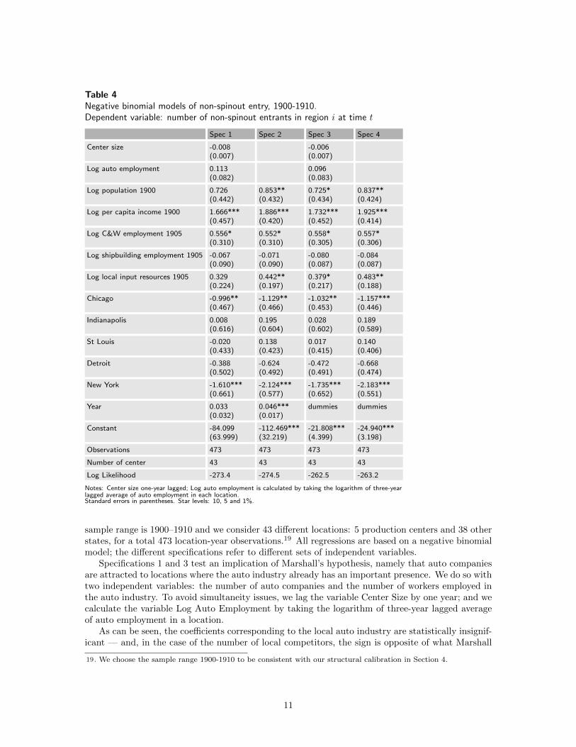
Table 4Negative binomial models of non-spinout entry, 1900-1910.Dependent variable: number of non-spinout entrants in region i at time t

Spec 1 Spec 2 Spec 3 Spec 4

Center size -0.008(0.007)

-0.006(0.007)

Log auto employment 0.113(0.082)

0.096(0.083)

Log population 1900 0.726(0.442)

0.853**(0.432)

0.725*(0.434)

0.837**(0.424)

Log per capita income 1900 1.666***(0.457)

1.886***(0.420)

1.732***(0.452)

1.925***(0.414)

Log C&W employment 1905 0.556*(0.310)

0.552*(0.310)

0.558*(0.305)

0.557*(0.306)

Log shipbuilding employment 1905 -0.067(0.090)

-0.071(0.090)

-0.080(0.087)

-0.084(0.087)

Log local input resources 1905 0.329(0.224)

0.442**(0.197)

0.379*(0.217)

0.483**(0.188)

Chicago -0.996**(0.467)

-1.129**(0.466)

-1.032**(0.453)

-1.157***(0.446)

Indianapolis 0.008(0.616)

0.195(0.604)

0.028(0.602)

0.189(0.589)

St Louis -0.020(0.433)

0.138(0.423)

0.017(0.415)

0.140(0.406)

Detroit -0.388(0.502)

-0.624(0.492)

-0.472(0.491)

-0.668(0.474)

New York -1.610***(0.661)

-2.124***(0.577)

-1.735***(0.652)

-2.183***(0.551)

Year 0.033(0.032)

0.046***(0.017)

dummies dummies

Constant -84.099(63.999)

-112.469***(32.219)

-21.808***(4.399)

-24.940***(3.198)

Observations 473 473 473 473

Number of center 43 43 43 43

Log Likelihood -273.4 -274.5 -262.5 -263.2

Notes: Center size one-year lagged; Log auto employment is calculated by taking the logarithm of three-yearlagged average of auto employment in each location.Standard errors in parentheses. Star levels: 10, 5 and 1%.

sample range is 1900–1910 and we consider 43 different locations: 5 production centers and 38 otherstates, for a total 473 location-year observations.19 All regressions are based on a negative binomialmodel; the different specifications refer to different sets of independent variables.

Specifications 1 and 3 test an implication of Marshall’s hypothesis, namely that auto companiesare attracted to locations where the auto industry already has an important presence. We do so withtwo independent variables: the number of auto companies and the number of workers employed inthe auto industry. To avoid simultaneity issues, we lag the variable Center Size by one year; and wecalculate the variable Log Auto Employment by taking the logarithm of three-year lagged averageof auto employment in a location.

As can be seen, the coefficients corresponding to the local auto industry are statistically insignif-icant — and, in the case of the number of local competitors, the sign is opposite of what Marshall

19. We choose the sample range 1900-1910 to be consistent with our structural calibration in Section 4.

11

Table 5A linear model explaining the explanatory variable C&WDependent variable: Log Carriage & Wagon Employment 1905

Spec 1

Log population 1900 0.648***(0.232)

Log per capita income 1900 -0.750*(0.425)

Log iron and steel 1905 0.341***(0.124)

Log lumber and timber 1905 0.083**(0.038)

Log brass and copper 1905 0.027(0.030)

Log rubber 1905 0.054*(0.031)

Constant -2.011(2.570)

Observations 43

R-squared 0.89

Notes: Robust standard errors in parentheses. Star levels: 10, 5 and 1%.

would predict.20 In other words, the regression results do not support the notion of Marshallianeconomies, at least the narrow notion of Marshallian economies.

Inspired by the work of Jacobs (1969) and Jackson (1988), we also consider the possibility ofa broader notion of agglomeration economies. Jacobs (1969) argues that the local presence of theshipbuilding industry played an important role in the emergence of Detroit as auto productioncenter. We test inter-industry agglomeration economies by measuring location-specific employmentin two related industries: carriage & wagon (C&W); and shipbuilding. The regression results showthat the former has a statistically significant effect, but not the latter.

Other location-level variables that appear statistically significant include: population, per-capitaincome and input availability. They show positive relations with the entry of non-spinout firms.

Considering that narrow Marshallian economies seem to play no role in auto firm entry decisions,our specifications 2 and 4 excludes the variables measuring local auto industry size (number of firmsand employment). Consistent with our expectation, the other variables’ regression coefficients arefairly close in value and in statistical significance.

Note that specifications 3 and 4 repeat specifications 1 and 2 with one difference: instead ofmeasuring a time trend we include year-specific dummy variables. While there is increase in fit(as measure by log likelihood), the difference is not very large. More important, the various pointestimates seem remarkably robust to changes in specification.

The local presence of the C&W industry, which we measure by total employment in each region,plays an important role in our agglomeration analysis. One possibility is that the size of the C&Windustry picks up the effect of local inputs, which are, to a great extent, shared with the autoindustry. In fact, early automobiles looked very much like horse carriages with an engine in lieu of ahorse. In this respect, our prior is confirmed by the Census of the U.S. Manufactures and Leontief’sinput-output table, which show the same top inputs for carriages and wagons as for cars: iron andsteel; lumber and timber; and rubber.

Table 5, where we regress C&W employment to the same set of input availability variables, also

20. We also ran alternative regressions in which the variable Log Auto Employment is dropped. The coefficientsof Center Size remain negative.

12

confirms the commonality of inputs.21 To the extent that the importance of inputs is not identicalfor the C&W and auto industries, Table 4, together with Table 5, allows us to tease out the “direct”and “indirect” effects of local inputs. The direct effect is given by the coefficient in Table 4; theindirect effect is given by the composition of the coefficient on inputs in Table 5 multiplied by thecoefficient on C&W employment in Table 4. We return to this in the next section, where we calibratea structural model of the auto industry.

Are spinouts an agglomeration force? About 17% of all firm entries in the history of the U.S.auto industry correspond to managers or employees of existing auto firms who leave the companyto start their own: a spinout. To the extent that spinout rates vary across regions, it is conceivablethat spinouts may act as a force toward agglomeration. We now consider a series of regressions totest this possibility.

Table 6 presents the results of four logit regressions, which differ in the set of independentvariables considered. The level of observation is firm-year and the sample range is 1900–1935, whichresults in a total of 3,000 to 3,500 observations approximately (depending on the set of independentvariables included). Some of the independent variables — center size, family size, center top andfamily top — are lagged one year. In this way, we avoid including the new entrants in the measureof existing firms. The variable Log Auto Employment is defined as before.

Some broad patterns emerge from this set of regressions. First, firm age has a positive andsignificant coefficient throughout. This suggests that older firms are more likely to give birth to aspinout than younger firms. Note that we do not include direct measures of firm quality on theright-hand side. For this reason, we expect firm age to capture firm capability to some extent, inwhich case the results suggest that higher capability firms are more likely to give birth to a spinout.

In addition to the parent’s characteristics (for which age is a proxy), the likelihood of giving birthto a spinout is also a function of the parent’s family. Specifications 1 and 3 suggest that the greatera firm’s family size, the more likely the firm will give birth to a new spinout. In specifications 2 and4 we use family top instead of family size. This alternative specification places extra weight on thequality of the parent’s family. The coefficient remains significant. It is higher in value, though weshould add that both the average and standard deviation of family top is lower than those of familysize.

Similarly to Table 4, Center Size or Center Top does not seem to have a significant correlationwith the dependent variable, as shown in specifications 1 and 2. However, when we include yeardummies instead of a year trend in the regressions (specifications 3 and 4), we do obtain a significantcoefficient, but it is negative, suggesting that, if there is a Marshallian effect, it is outweighed bythe competition effect. The other measure of local auto industry size, Auto Employment, showsa positive correlation with spinout entry in specifications 1 and 2, but the sign turns negative inspecifications 3 and 4 when year dummies are used, again contradicting to the positive Marshallianeconomies.

Controlling for firm age and family characteristics, we find local factors (e.g. population, income,related industries and input resources) have no significant effect on the dependent variable. Thissuggests that firm age and family are sufficient and more direct predictors of firm quality than thoselocal factors.

In the first two specifications, we use a year trend as an explanatory variable. The negativecoefficient reflects the fact that entry became more difficult as auto evolved into a mature industryat later stages. Since the evolution is not linear, in specifications 3 and 4 we use year dummiesinstead of the year trend. Notwithstanding these changes, our estimate of the relevant coefficientsare similar.

Last but not least, the Detroit dummy shows much larger effect than other location dummies,

21. The regression coefficients are unlikely to result from any reverse causality given that the inputs used inC&W production were quite small compared with the size of the input sectors. Nationwide, in 1905, iron andsteel used in C&W accounted for 0.45% of total iron and steel production; the corresponding percentage forlumber and timber was 1.78%; and for rubber, 4.17%.

13

Table 6Logit models of spinout entry, 1900-1935.Dependent variable: firm gives birth to spinout at time t


Firm age 0.083***(0.028)

0.074***(0.028)

0.093***(0.029)

0.082***(0.030)

Center size -0.009(0.015)

-0.037*(0.022)

Family size 0.160***(0.052)

0.183***(0.057)

Center top -0.079(0.092)

-0.164*(0.099)

Family top 0.299***(0.096)

0.311***(0.095)


0.404*(0.232)

-0.217(0.292)

-0.104(0.281)


0.021(0.578)

-0.667(0.650)

-0.556(0.540)

Log per capita income 1900 -2.375(2.067)

-2.487(2.098)

-1.347(1.856)

-1.441(1.841)

Log C&W employment 1905 -0.105(0.563)

-0.246(0.549)

0.739(0.764)

0.539(0.694)

Log shipbuilding employment 1905 -0.036(0.193)

-0.037(0.193)

-0.044(0.188)

-0.045(0.184)

Log local input resources 1905 -0.089(0.535)

-0.073(0.545)

0.285(0.460)

0.226(0.441)

Chicago 0.717(0.671)

0.717(0.631)

1.146(0.816)

0.677(0.636)

Indianapolis 0.116(0.717)

0.118(0.667)

0.594(0.899)

0.067(0.683)

Detroit 1.049(0.778)

1.589(1.250)

2.713**(1.256)

3.174**(1.485)

Rochester 0.615(0.737)

0.672(0.735)

0.788(0.738)

0.651(0.681)

New York City 1.210(0.795)

1.296(0.816)

1.756**(0.857)

1.485**(0.736)

Year -0.156***(0.055)

-0.157***(0.051)

dummies dummies

Constant 303.441***(109.951)

306.573***(102.463)

-3.161(10.257)

-1.144(9.686)

Observations 3,475 3,475 2,979 2,979

Notes: Center size, Family size, Center top and Family top one-year lagged; Log auto employment is calculatedby taking the logarithm of three-year lagged average of auto employment in each location.Robust standard errors clustered by firm. Star levels: 10, 5 and 1%.

14

especially in specifications 3 and 4.22 Moreover, the coefficient’s size is also quite significant incomparison to other determinants of spinout entry. For example, being in Detroit increases theprobability of giving birth to a spinout by more than a 5 standard deviation increase in firm age oradding 10 top firms to a firm’s family (specification 4).

For robustness checks, we also repeat the regressions by extending the sample range to 1895-1942while dropping the variable Log Auto Employment (the data of auto employment is available up to1935). All the relevant results remain unchanged.

Survival of the fittest: determinants of exit rates. As happens in many industries, net entry andexit rates in the auto industry are considerably lower than gross entry and exit rates. Consequently,understanding exit patterns is an important step towards understanding the evolution of industryconcentration. Our next set of results pertains precisely to firm exit.

Table 7 displays the results of four logit regressions. In all of them, the dependent variable isfirm exit, that is, a dummy variable that takes the value 1 if a firm exits in a given year. Differentspecifications correspond to different sets of independent variables. Some of the independent vari-ables — center size, family size, center top and family top — are lagged one year, and the variableLog Auto Employment is defined as before.

In all regressions, firm age has a negative coefficient. This is consistent with much of the previousliterature on firm exit: older firms are less likely to exit than younger firms. The results also showthat other things being equal, de alio and spinout firms are less likely to exit than de novo firms.

We saw earlier that center size does not seem to have a big impact on firm entry (cf Tables 4and 6). Table 7 suggests that center size may instead have a slightly positive effect on firm exit(specification 3), while the effect of center top is not significant. Auto Employment shows a positiveeffect on firm exit, and the effect becomes statistically significant in specifications 3 and 4. Again,the evidence does not seem to match the prediction of Marshall-type agglomeration economies inthe strict sense. By contrast, family size and family top both show significant positive impact onfirm survival in all specifications.

After we control for firm age and family, most other local factors do not show a significant effecton the dependent variable (except population and C&W employment in specifications 3 and 4).Again, this suggests that firm age and family are sufficient and more direct predictors of firm qualitythan those local factors.

Finally, the various center dummies suggest that there are some remaining location specificeffects, with firms in Indianapolis and Detroit more likely to survive than firms in other regions.

All in the family: determinants of spinout performance. Several of the above regressionssuggest that “family matters.” Specifically, the size and quality of a family has an important impacton whether a spinout will take place and whether such spinout will survive. We now take a closerlook at the mechanism whereby family membership helps the survival of a spinout firm.

In our data, a small portion of spinout firms happened to locate away from their parents, largelydue to exogenous reasons.23 Comparing the performance of these spinouts with those locating nearbythe parents allows us to address the above question. Table 14 in the Appendix displays four logitregressions where the dependent variable, as in the previous table, is firm exit. Differently fromthe regressions in Table 7, we now split the family size and family top variables by location: localfamily size now measures the number of relatives in the same location, whereas non-local familysize measures the number of relatives located elsewhere (a similar distinction applies to local andnon-local family top).

The results are quite striking: whereas the local variables (family size and family top) are sta-tistically significant, the non-local ones are not statistically significant. In terms of coefficient size,

22. St. Louis is omitted in the regressions due to the inexistence of any spinout.23. We investigate whether there could be endogeneity bias related to spinouts’ location choices, for instance,

whether certain types of spinouts tend to move away from their parents. In doing so, we collected detailedinformation on the motive of every spinout from the top three families: GM/Buick, Ford and Oldsmobile.The results show no systematic bias between the motive of a spinout and its subsequent location choice.

15

Table 7Logit models of firm exit, 1900-1935. Dependent variable: firm exit at time t


Firm age -0.070***(0.010)

-0.061***(0.009)

-0.078***(0.010)

-0.069***(0.010)

De Alio -0.457***(0.108)

-0.452***(0.106)

-0.479***(0.108)

-0.469***(0.105)

Spinout -0.429***(0.155)

-0.222(0.159)

-0.421***(0.159)

-0.219(0.161)

Center size 0.009(0.006)

0.014*(0.007)

Family size -0.086**(0.037)

-0.106**(0.042)

Center top 0.017(0.033)

0.018(0.034)

Family top -0.355***(0.073)

-0.391***(0.080)


0.066(0.058)

0.133**(0.065)

0.153**(0.067)


0.196(0.165)

0.283*(0.165)

0.311*(0.163)

Log per capita income 1900 0.354(0.304)

0.330(0.307)

0.174(0.318)

0.112(0.316)


-0.161(0.141)

-0.263*(0.150)

-0.315**(0.145)

Log shipbuilding employment 1905 0.026(0.045)

0.034(0.045)

0.011(0.049)

0.021(0.049)


-0.090(0.111)

-0.113(0.112)

-0.120(0.114)

St Louis 0.179(0.315)

0.272(0.318)

0.040(0.316)

0.182(0.306)

Chicago -0.267(0.223)

-0.116(0.194)

-0.374(0.242)

-0.118(0.195)

Indianapolis -0.546**(0.266)

-0.404*(0.228)

-0.669**(0.291)

-0.419*(0.235)

Detroit -0.657**(0.300)

-0.375(0.487)

-0.931***(0.362)

-0.457(0.505)

Rochester -0.375(0.286)

-0.330(0.275)

-0.443(0.286)

-0.341(0.270)

New York City -0.028(0.220)

0.097(0.206)

-0.111(0.234)

0.126(0.206)

Year 0.024(0.015)

0.017(0.014)

dummies dummies

Constant -48.243(29.541)

-34.741(27.057)

-0.385(1.942)

-0.121(1.936)

Observations 3,573 3,573 3,537 3,537

Notes: Center size, Family size, Center top and Family top one-year lagged; Log auto employment is calculated

by taking the logarithm of three-year lagged average of auto employment in each location.Robust standard errors clustered by firm. Star levels: 10, 5 and 1%.

16

local family top shows greater values (in absolute terms) than family top in Table 7. In fact, whenwe include local family top (specifications 2 and 4 in Table 14) the variable spinout ceases to bestatistically significant. This suggests that belonging to a family of high performance firms andbeing located nearby family relatives is associated with superior spinout performance, whereas if afirm is located far from its family then performance is not statistically different from that of de novoentrants. The finding suggests that spinouts may actually benefit from intra-family local spilloversrather than the heredity effect, which clarifies the conflicting views between Marshall and Klepper.

Robustness analysis and further notes. We perform a series of robustness checks on our resultsregarding firm exit. First, we consider alternative treatments of exit. In our exit regressions, wedid not separate exit by acquisition from exit by liquidation. It may be argued that exit by beingacquired should not be counted as firm failure (in some cases, it may be quite the opposite).24

One way to solve the potential problem of confounding the two types of exit is to count exits byacquisition as censored observations of exits. Under the alternative specification, the regressionresults are similar in signs and values but even stronger in statistical significance.

Second, in our spinout and exit regressions we did not include top firm as an explanatory variable.The reason is that we would like the explanatory variables (e.g. center size, family size, etc) topredict the firm’s performance in terms of spinout and exit. Top firm is just another measure offirm performance, which duplicates the dependent variables. Of course, top firm itself could be animperfect proxy for firm performance (the way we define it as ever being a top firm). Therefore,when we do include it as an explanatory variable, our results still hold in terms of coefficient signsand values but become statistically weaker.

Our exit regressions pool spinout and non-spinout firms (with a dummy for spinout firms). Oneadvantage of this approach is that it takes into account the possibility that spinout and non-spinoutfirms are subject to the same survival factors. As an alternative, we also ran separate exit regressionsfor spinout and non-spinout firms. The results for the separate regressions, which we include inTables 15 and 16 in the Appendix, are qualitatively and quantitatively similar. One interestingfinding is that Auto Employment shows a negative effect on spinout firm exit, but a positive effecton non-spinout firm exit. This is consistent with our previous findings in the sense that the measureof local auto employment may proxy for local family size of spinout firms, but for non-spinout firmsit may instead reflect the presence of competitors.

Finally, for robustness checks, we repeat the exit regressions by extending the sample range to1895-1942 while dropping the variable Log Auto Employment. The results are very similar.

Summary of main empirical results. We may summarize our empirical findings as follows:

• Entry rates by non-spinout firms in a given location are increasing in: (a) regional populationand income; (b) regional employment levels in the C&W industry; (c) local input resources.

• Spinout entrants are more likely to come out of: (a) older firms; (b) larger and better families;(c) Detroit.

• Firm survival rates are higher if: (a) the firm is older; (b) the firm resulted from de alio entry;(c) the firm was spun out of a high-performance parent and remained in the same location asthe parent; (d) the firm is located in Detroit or Indianapolis.

• Firm entry and survival rates do not depend on measure of other auto firms in the samelocation. If anything, spinouts are negatively impacted and exits are positively impacted bycompetitors (cf Tables 6, 7 and 14).

Taken together, the evidence casts doubt on Marshall (1890) type intra-industry externalities inthe strict sense. Rather, Jacobs (1969) type co-agglomeration economies and Klepper (2007) type

24. The data show that in the sample range 1895-1942, there were 108 exits (or 14% of all exits during theperiod) resulting from acquisition.

17

spinout entry appear relevant, but they may actually work through the Marshallian externalities ina broader context. Finally, as suggested by the work of Ellison and Glaeser (1999), the results alsounveil some significant location fixed effects, particularly due to local input resources.

The reduced-form analysis is useful for getting a first glance at the sign and size of the variouseffects. It also provides a useful springboard for our next step: to develop and calibrate a structuralmodel of the U.S. auto industry. Such a model will allow us to perform a series of counterfactualexercises to evaluate the relative weight of each force of industry agglomeration.

4. A quantitative model of the U.S. auto industry

In this section, we develop a simple model of industry dynamics in the spirit of Hopenhayn (1992)which generates theoretical predictions consistent with our reduced-form analysis. We then use thecalibrated model to quantify the contribution of each agglomeration factor.25

In the model, firms are forward looking, competitive price takers producing a homogeneousproduct with heterogeneous production capabilities. We consider two types of entrants: de novoentrants and spinout entrants.26 De novo entrants originate outside of the industry. Spinout entrants,by contrast, are founded by former industry participants, that is, managers or workers previouslyemployed by an existing industry participant.

We assume that the “supply” of de novo entrants is affected by location-specific characteristics.Regarding spinout entrants, we assume that each incumbent firm generates potential spinouts ata constant per period rate. However, just as with de novo entrants, a potential spinout makes anoptimal entry decision. In other words, every actual and potential firm is treated as a rational,forward-looking agent who makes optimal entry and exit decisions.

We also make the assumption that a spinout shares the same capability with its parent firm andchooses the same location as the parent. The model does not restrict the source of the hereditaryeffect: it could result from interactions of member firms within the family network (e.g., throughknowledge linkages or business relations) rather than the family-specific capability that reflectscommon “genes.”27

With all of these ingredients, we perform an agglomeration accounting exercise where we considerthe four components listed in the paper’s title: competitors, complementors, parents and places. By“competitors” we mean Marshallian economies in the strictest sense of the word: the presence ofother local firms from the same industry. By “complementors” we mean the broader perspective ofinter-industry agglomeration economies: the effect of local related industries. By “parents” we meanthe effect of spinouts in creating the self-reinforcing dynamics of geographical location. Finally, by“places” we mean local conditions such as income and the availability of production inputs.

As mentioned in Section 2, one remarkable feature of the U.S. auto industry is the significantshakeout it went through between the mid-1910s and the early 1930s. Many authors have focused onindustry shakeouts, both theoretically and empirically, dealing both with the auto industry and otherindustries. Our focus is in explaining geographical agglomeration rather than shakeout. Accordingly,we consider a stationary model and calibrate it with pre-shakeout data (census years 1909 and 1914).

25. Alternatively, one may consider using a reduced-form analysis for explaining/predicting auto outputs acrosslocations. However, reduced-form analysis has its limitations, especially when it comes to identify theendogenous channels (e.g., intra-industry spillovers or spinouts) that affect the output distribution. Becauseour paper considers intra-industry spillovers, inter-industry spillovers, local conditions and spinouts as fourdifferent forces affecting the auto industry agglomeration, a structural analysis is well suited for disentanglingthese forces and quantifying their relative importance.

26. For simplicity, we conflate de novo and de alio entry into one single category: de novo. We do so for tworeasons. First, it keeps our structural model simpler. Second, to the extent that we include C&W andshipbuilding employment for estimating the quality of non-spinout entry in each location (cf Table 8: being atop non-spinout entrant), we effectively allow related industries to influence the quality of non-spinoutentrants in our calibration of the structural model.

27. Our reduced-form analysis strongly suggests that the former is more important than the latter. However, forthe purposes of the agglomeration accounting exercise we preform in this section, this distinction is irrelevant.

18

We note that by the early 1910s no major shakeout had yet occurred, but significant agglomerationhad already taken place, including the concentration of production in Detroit.28

In the remainder of this section we do three things. First, we develop a dynamic model withthe above properties. Second, we calibrate the model based on the coefficients obtained in ourreduced-form regressions. Finally, we perform a series of counterfactual simulations where each ofthe model’s features is “shut down.” In this way we are able to estimate the contribution of eachof the four features (competitors, complementors, parents and places) to explaining the observedindustry agglomeration, including its ultimate concentration in Detroit.

Individual firm’s problem. The model is cast in discrete time and infinite horizon. A continuumof firms produce a homogenous good in a competitive market. Each firm is indexed by its discretecapability s ∈ {0, 1, ..., s} and location j. For simplicity, we assume that a firm with capability sstarting at location j will retain the same capability and operate at the same location for the rest ofits life. The industry structure is thus summarized by mt(s, j), the total mass of firms of capabilitys at location j time t. Given our assumption regarding capability and location, the evolution ofmt(s, j) is entirely governed by entry and exit, the main focus of our analysis.

In each period, incumbent firms engage in product market competition by taking the industryprice pt as given. Each firm chooses optimal output q(s; j, pt,m

jt ) based on its capability and location

characteristics. Location characteristics include the number of firms in location j, mjt , as well as

other factors.29 Their period profit is denoted by π(s; j, pt,mjt ). We assume q(s; j, pt,m

jt ) and

π(s; j, pt,mjt ) are continuous, bounded, and strictly increasing in s and pt.

30

Once an incumbent firm obtains its profit, it decides whether to continue operating or insteadto leave the industry and earn an outside options φx. The value of the outside option is privatelyknown by the firm and i.i.d. according to cdf F (φx). Given its belief of a time-series sequence ofindustry price p and mass of firms at own location mj , an incumbent’s problem can be defined as:

Vt(s; j, p,mj , φx) = π(s; j, pt,m

jt ) + max{VC t, φ

x},

where the value of continuation is

VC t(s; j, p,mj) = β

∫Vt+1(s; j, p,mj , φ

x) dF (φx).

Potential entrants at each location make their entry decisions at the same time as incumbents.As mentioned earlier, we consider two types of entrants: de novo and spinout. De novo entrantsoriginate outside the industry. We assume the total mass of potential de novo entrants at locationj, Mj , is determined by location-specific characteristics. Each potential de novo entrant in locationj faces a sunk entry cost φej . If the potential entrant pays φej then it is given an initial draw ofcapability s from the distribution µ(s, j), the discrete density function of capability s at locationj. Hence, a potential entrant’s probability of entry is given by Ψj

t , the probability that the ex-anteexpected value of incumbency is greater than the entry cost φej . It follows that the expected number

28. We calibrate our model to the average regional auto output shares between 1909 and 1914. Because theregional shares were stable during this period, the results do not change if we instead calibrate our model toany specific year.

29. For simplicity, we normalize input price to be unit in every location, so a firm that faces lower input pricesdue to better access to local inputs or related industries would show up as having higher capability, and alocation that enjoy an abundance of local inputs or related industries would show up as having a higherfraction of high-capability entrants. Because we feed the structural model with quantity and quality ofentrants from the reduced-form regressions, the effect of lower input prices, while not explicitly modeled, iscaptured by our model simulation.

30. It is less straightforward to make assumptions about the relationship between profit and the local mass offirms mj

t . We will assume that the force of agglomeration is not too strong such that a stationary industryequilibrium exists. Detailed magnitude of the intra-industry agglomeration force is discussed in ourquantitative exercise.

19

of de novo entrants at location j is given by

njt = ΨjtMj = Pr

(∑s

VC t(s; j, p,mj)µ(s, j) ≥ φej

)Mj . (1)

The second type of entrants, spinouts, originate within the industry. Each period, an incumbentfirm at location j has a probability γjt of generating a potential spinout. We assume the potentialspinout shares the same capability s with its parent and knows its capability when making the entrydecision. As a result, the spinout’s entry decision is equivalent to its parent’s continuing decision:31

A potential spinout will enter if its entry value is higher than its random outside option φx, i.e.,

VC t(s; j, p,mj) ≥ φx.

We assume that if a potential spinout entrant chooses not to enter in the current period, then theopportunity is foregone forever.32

Note that there are two important differences between the two types of entrants. First, whilepotential de novo entrants are uncertain about their capability of operating in a new industry,spinout entrants directly inherit their parent’s capability draw. This is a sharp assumption we maketo highlight the fact that spinout entrants have better knowledge of their own capability given bytheir industry experience. Second, we assume that de novo entrants need to pay an additional entrycost φe with respect to spinouts, a difference that corresponds to the extra investment de novoentrants need to make to build up business relations or a customer base.

Supply and demand. We next derive the transition of the mass of firms of capability s at locationj. This transition depends on the number of exits, spinouts, and de novo entrants at each state (s, j).Specifically, we have

mt+1(s, j) = mt(s, j) (1 + γjt )χs,jt + njtµ(s, j), (2)

whereχs,jt = F

(VC t(s; j, p,mj)

)(3)

is the probability of staying in the industry given the cdf function F of the outside option.The right-hand side of (2) reflects the two sources of entry mentioned earlier. The first term

combines the decisions of incumbents and spinout entrants. There are in total mt(s, j) (1 + γjt ) suchfirms making entry decisions, mt(s, j) incumbents and mt(s, j) γ

jt potential spinout entrants. Since

their continuation value is the same, their continuation/entry probability, χs,jt , is also the same. Thesecond item on the right-hand side is the inflow of de novo entrants. Note that the number of denovo entrants, njt , is location specific, and de novo entrants at location j are ex ante identical interms of their expected capability.

Given each firm’s output level, q(s; j, pt,mjt ), and given the mass of each firm’s type, mt(s, j), we

determine total supply in location j. Aggregating over locations, we get total supply in the industry.We assume industry demand is given by the inverse demand function p = D−1(Q). Industry pricethen clears the market in each period so that total supply equals total demand:

pt = D−1

∑s,j

q(s; j, pt,mjt ) mt(s, j)

. (4)

Industry equilibrium. An industry equilibrium is defined by a sequence of prices p∗, a mass ofentrants n∗jt, a measure of incumbent firms m∗(s, j, t), and a policy function χ∗(s, j, t) such that

31. Our assumption that the continuation decision of an incumbent and the entry decision of its spinout areequivalent captures the family network effect found in our reduced-form regressions.

32. This is a simplifying assumption that allows us to maintain a constant spinout rate (per firm and per period).Departing from this assumption would require us to keep track of a cumulative pool of heterogeneouspotential spinouts, leading to an unmanageable state space.

20

• n∗jt satisfies the entry condition for de novo entrants each period, that is, n∗jt satisfies (1);

• m∗(s, j, t+ 1) is defined recursively given m∗(s, j, t), n∗jt, and χ∗(s, j, t), according to (2).

• χ∗(s, j, t) solves incumbent firms and potential spinouts’ dynamic optimization problem eachperiod, given their belief of p∗ and m∗j , that is, χ∗(s, j, t) satisfies (3);

• p∗t clears product market each period, that is, p∗t satisfies (4);

In the following analysis, we consider a stationary industry equilibrium.33 Although our modelintroduces some specific features — namely the distinction between de novo and spinout entrants —its basic features are similar to (and simpler than) the general framework presented in Hopenhayn(1992). With small changes, the equilibrium existence and uniqueness results in Hopenhayn (1992)can therefore be applied in the present context.

Equilibrium properties. The theoretical model presented above implies a series of equilibriumproperties which we now develop formally (the proofs are in the Appendix).

Proposition 1. An incumbent (a potential spinout) is more likely to survive (enter) if it belongs toa higher capability family, given the same location and time.

Proposition 2. A high-capability family on average has a bigger family size, given the same locationand time.

Proposition 3. Given positive entry and exit in the stationary equilibrium, spinout firms have lowerprobability of exit than de novo firms, given the same location and time.

All of these results are consistent with the empirical evidence presented in Section 3. For example,Table 6 shows that family top has a positive effect on spinout rates, while Table 7 shows that familytop has a negative impact on exit rates (cf Proposition 1). Propositions 1 and 2 together implythat family size is positively correlated with the spinout rate but negatively correlated with the exitrate, which are consistent with our findings in Tables 6 and 7. Moreover, Tables 7 and 14 show thatspinouts have a lower exit rate than de novo firms (cf Proposition 3).

This correspondence between theory and empirical observation gives us confidence in the modelas a good description of the auto industry. We next attempt to calibrate the model’s parameterswith a view at going beyond qualitative description. Specifically, our goal is to use the calibratedmodel to estimate the relative contribution of each of the model’s features, an exercise we referto as “agglomeration accounting.” We consider four possible sources of agglomeration economies:intra-industry effects, inter-industry effects, spinouts, and location specific effects (particularly thelocal inputs).

Functional forms. In the model calibration, we consider 43 locations (j = 1, ..., 43), correspond-ing to five production centers (i.e. Chicago, Detroit, New York, Indianapolis and St. Louis) and 38non-center states;34 and two levels of firm capability (s = 1, 2), corresponding to low and high. Weexclude any location fixed effects in production functions so as to limit the number of free param-eters. Instead, we allow for location-specific effects through differences in entry and spinout ratesand types.

We specify the profit function π(s; p,mj) by assuming a decreasing returns production function

q(s) = [exp(c1 s)mηj ] lα, (5)

33. Naturally, long-run changes in the auto industry can be viewed as comparative statics of the stationaryequilibrium. In the Appendix, we show that the model is amenable to rescaling so that any changes to marketsize or production technology can be modeled equivalently as changing the value of firms’ outside option.

34. We combine New York City and Rochester into one center (New York). We also assume that non-centerlocations are identical.

21

where c1 captures the relative advantage of firms with a higher capability, and l is the quantity ofinput. (We normalize the input price wl=1, so a firm that faces a lower value of wl would simplyshow up as having a higher capability s.) The elasticity η measures the strength of intra-industryspillover. This implies that a firm, taking industry price p as given, has profit and output given by

π(s; p,mj) =

(1− αα

)(αp)

11−α

[exp(c1 s)m

ηj

] 11−α , (6)

q∗(s; p,mj) = (αp)α

1−α[exp(c1 s)m

ηj

] 11−α . (7)

Furthermore, we assume that the outside option follows an i.i.d. exponential distribution with pa-rameter σ.

Demand curve. We estimate an industry demand function using historical annual data of averagecar price and output from Thomas (1977). The data range is 1900–1929, and we assume a simplelog-log per capita demand function:

log

(Qtpop t

)= at − b log(pt).

In the regression, we control for log U.S. GDP per capita (as a proxy for income) in the demandintercept at. Both car price and GDP per capita are in real terms.

To address the issue of potential endogeneity of the price variable, we exploit the model struc-ture. In our theoretical model, industry long-run capability distribution is correlated with price,yet uncorrelated with any transitory demand shock. One proxy for long-run industry capabilitydistribution is the share of spinout firms, which we used as an instrumental variable to estimatethe demand slope parameter b. Our IV estimation gives b = 3.39 (0.39), with standard error inparentheses. The demand shifter is given by at = 0.04× log(GDP per capita)t + 17.40.

The first-stage regression results (adj. R2 = 0.86) are given by

log(pt) = 2.86(1.28)

+ 1.72(0.76)

× log

(GDPtpop t

)− 5.89

(0.66)× (Spinout Share)t.

The second-stage regression results (adj. R2 = 0.83) are in turn given by

log

(Qtpop t

)= 17.40

(5.55)+ 0.04

(2.17)× log

GDPtpop t

− 3.39(0.39)

× log(pt),

where standard errors are reported in parentheses.

Calibration. We observe positive de novo entrants at each location during our sample period.Since all firms compete in a single auto market, the observed entry pattern by location can berationalized by a free entry equilibrium with location-specific Mj and Ψj

t . Empirically, we assume theobserved quantity of de novo entrants in location j, nj , is explained by the reduced-form regressionsin Section 3 through local factors such as population, income, related-industries employment andinput resources. We thus feed into the model the estimated average non-spinout entry rates in eachlocation (as explained by our negative binomial regression reported in Table 4, Spec 2), that is, nj .

35

In order to quantify the difference between high- and low-quality entrants, in Table 8 we reportthe results of a series of logit regressions where the dependent variable is non-spinout top entry, thatis, we model the probability of entry by a non-spinout firm that becomes a top firm (according to

35. The regression results reported in Table 4 suggest that intra-industry externalities are quantitativelynegligible in explaining entry by non-spinout firms, so we use Spec 2 of Table 4 to simulate non-spinoutentrants in our model calibration and counterfactual exercises.

22

Table 8Logit models of top non-spinout entry, 1900-1910.Dependent variable: being a top non-spinout entrant

Spec 1 Spec 2 Spec 3

Entry year -0.293***(0.097)

-0.326***(0.110)

-0.325***(0.109)

Log population 1900 -0.351(0.295)

-4.197**(1.924)

-4.673*(2.748)


4.175(6.025)

4.762(7.592)

Log C&W employment 1905 3.275**(1.655)

3.311*(1.827)


0.271(0.713)


Constant 567.034***(187.758)

600.161***(209.409)

592.731***(212.195)

Observations 461 461 461

Log Likelihood -63.50 -57.49 -57.45

Notes: Standard errors in parentheses. Star levels: 10, 5 and 1%.

our definition of top firm). The sample range is 1900–1910; it includes 461 non-spinout entrants in 5production centers and 38 other states. The results suggest that the relative size of the carriage andwagon (C&W) industry, measured by local C&W employment relative to population, significantlyraises the chance of being a top non-spinout entrant. Judging from the value of log likelihood, themodel fit is equally good whether we include input-relevant resource availability (Spec 3) or not(Spec 2). We use the results from specification 3 to calibrate the average entry probability of high-and low-capability firms in each location, that is, µ(s, j).

So as to quantify the effect of intra-industry spillovers (Marshallian economies, in the strictsense), Table 9 shows the results of a series of regressions with log average output value per firm(in region j) as a dependent variable. We allow firm output to be affected by the number of localcompetitors through the elasticity parameter η/(1−α) in the output function, as in (7). We estimateη/(1 − α) = −0.26. This negative value is consistent with the negative intra-industry spillovers wefound in the reduced-form entry and exit regressions.36

We set the discount factor at β = 0.925. This leaves five key model parameters to be calibrated:the parameter reflecting cost heterogeneity across types, c1; the degree of returns to scale, α; theaverage value of the outside option, σ; the industry average spinout birth probability, γ; and theDetroit specific spinout birth probability, γ

D. Our calibration strategy considers 1909–1914 as an

industry equilibrium, where the industry agglomeration pattern was relatively stable. We calibratethe parameter values to match the following data moments, as shown in Table 10:

• the distribution of output across the five production centers and other regions

• the firm exit rate at the five production centers and other regions

• the spinout rates at the five production centers and other regions

Intuitively, our model moments of output distribution and firm exit rates across locations are largely

36. For robustness checks, we also consider smaller intra-industry spillover effects. For instance, we re-ran themodel calibration and counterfactual analysis by assuming η = 0, in which case the effect of intra-industryspillovers is set to zero by construction. The results are reported in the Appendix (Tables 17-20).

23

Table 9Average output value per firm.Dependent variable: logarithm of average output value per auto firm in region j at time t

Sample period 1899–1910 1899–1919 1899–1935

Log center size -0.255(0.154)

-0.258***(0.086)

-0.274***(0.080)

Log population 1900 0.480***(0.136)

0.750***(0.098)

0.893***(0.131)


0.641**(0.251)

1.098***(0.262)

Log C&W employment 1905 0.351**(0.160)

0.326***(0.095)

0.451***(0.103)

Log shipbuilding employment 1905 -0.205***(0.042)

-0.242***(0.032)

-0.109**(0.042)

Log iron and steel 1905 -0.201(0.222)

-0.371***(0.114)

-0.567***(0.129)

Log lumber and timber 1905 -0.015(0.077)

0.099**(0.045)

0.050(0.049)

Log brass and copper 1905 0.059(0.085)

0.049(0.036)

0.062*(0.034)

Log rubber 1905 0.155***(0.025)

0.163***(0.017)

0.131***(0.019)

Year dummies Included included Included

Constant 8.168**(3.254)

3.913**(1.815)

3.197*(1.857)

Observations 132 283 430

R-squared 0.563 0.828 0.881

Notes: Standard errors in parentheses. Star levels: 10, 5 and 1%.

24

determined by the parameters c1, α and σ, while the spinout rates are mainly driven by γ and γD

.To best match the data, we set c1 = 0.6, α = 0.7, σ = 1.96, γ

D= 0.08, and γ = 0.02; the fit is very

good, as shown in the following analysis.Note that the calibrated value of σ, the average value of a firm’s outside option, summarizes the

effects of the market demand and production technology in the model. In fact, we provide a proofin the Appendix that the industry equilibrium derived from our model is invariant with respect toa rescaling of market size a or production technology q(s), as long as σ is rescaled appropriately.Therefore, by adjusting the value of σ, we do not need to calibrate any scaling parameters in themarket demand function and the production function.

The calibrated values of γD

and γ suggest that Detroit had a substantial advantage in generatingspinouts. Marx, Strumsky and Fleming (2009) offer a possible explanation for this pattern: Michiganwas one of the few states that banned employee non-compete contracts at the time, which in turnencouraged the formation of spinout firms.37

Agglomeration accounting: short-run analysis. As mentioned in Section 3, there are two ways oflooking at the effect of local conditions and co-agglomeration. Auto entrants are more likely to foundin locations with more workers in the C&W industry. This implies that local factors (population,income, input resources) have an effect on entries into the auto industry in two ways: directly, to theextent that better inputs make for more profitable entry; and indirectly, to the extent that betterinputs attract more firms and workers into the C&W industry, which in turn increases the entryrate into the auto industry.

In other words, we may distinguish between a “short-run” and a “long-run” agglomeration ac-counting exercise. In our short-run decomposition, we take the location decisions in the C&Windustry as given; by contrast, in our long-run decomposition, we account for the effect of localconditions on the location’s C&W industry size. We expect that our long-run accounting will assigna greater weight to local factors (which we treat as exogenous). The question is, how much greater.

Table 10 presents the results from our short-run decomposition exercise. The second columnshows the data, whereas the third column shows the basic model fit. Following that, we have 6columns which correspond to different counterfactuals. In order to judge the goodness of fit, wepresent several basic variables of interest related to agglomeration accounting:

• Each region’s auto output share

• The HHI index applied to each region’s auto output share, that is, HHI =∑s2i , where si is

region i’s output share

• The prediction mean squared error for the cross-location output distribution

Additional variables of interest include

• Exit rates (Detroit and Non-Detroit)

• Ex post spinout rates (Regional average and Detroit top firms)

37. According to Marx, Strumsky and Fleming (2009),

At the turn of the 20th century, the metropolitan area of Detroit, Michigan, in many waysresembled the Silicon Valley of the last few decades. Growth of the nascent auto industry wasexplosive ... Ten years prior, the Michigan legislature in 1905 had passed statute 445.761(bearing resemblance to California’s prohibition): “All agreements and contracts by which anyperson agrees not to engage in any avocation or employment are hereby declared to be againstpublic policy and illegal and void.” This law governed non-compete enforcement until March 27,1985, when the Michigan Antitrust Reform Act (MARA) repealed section 445 and with it theprohibition on enforcing non-compete agreements.

Related, Franco and Mitchell (2008) study more recent high-tech industries and argue the overtaking ofRoute 128 by Silicon Valley can be explained by the difference in noncompete policy between Massachusettsand California.

25

Table 10Short-run decomposition. Model fit and six counterfactuals: 1. No intra-industry externalities; 2.Uniform C&W employment levels; 3. Uniform input resources; 4. Uniform other factors (population,income, shipbuilding, location dummies etc); 5. No spinout; 6. No Detroit-specific spinout rate

Counterfactuals

Data Model 1 2 3 4 5 6

Output share

Chicago 0.060 0.037 0.028 0.037 0.028 0.038 0.074 0.066

Detroit 0.670 0.681 0.798 0.449 0.575 0.659 0.262 0.239

New York 0.140 0.081 0.067 0.054 0.032 0.192 0.166 0.148

Indianapolis 0.070 0.066 0.044 0.030 0.094 0.020 0.163 0.154

St Louis 0.010 0.011 0.008 0.021 0.021 0.009 0.022 0.019

Others 0.060 0.125 0.055 0.409 0.250 0.081 0.313 0.374

HHI 0.477 0.476 0.644 0.211 0.343 0.474 0.131 0.111

Prediction MSE 0.001 0.004 0.030 0.010 0.001 0.040 0.049

Exit rate

Non-Detroit 0.150 0.133 0.137 0.132 0.133 0.136 0.121 0.122

Detroit 0.130 0.112 0.107 0.116 0.106 0.108 0.119 0.123

Additional moments

Average regional spinout rate 0.030 0.044 0.047 0.038 0.038 0.041 0 0.018

Detroit top spinout rate 0.079 0.074 0.074 0.074 0.074 0.074 0 0.019

Finally, in order to account for the effect of each model feature, we run alternative counterfactualswhere that feature is shut off. This is done by adjusting the feed of nj and µ(s, j) from our reduced-form regressions, while keeping other model parameters unchanged.38 The results are shown in thelast 6 columns in Table 10. In Counterfactual 1, we set η = 0, that is, we assume the presence oflocal auto companies has no effect on an auto firm’s production function. In other words, we assumeno intra-industry Marshallian effects. In Counterfactual 2, we set the variable “C&W industryemployment” to have the same value in all regions (specifically, the average of production centers)when estimating the number and quality of de novo entrants based on the reduced-form regressions(cf Table 4, Spec 2; Table 8, Spec 3); and then feed those into our structural model to recomputethe equilibrium. We thus effectively shut off the type of related industries effects described in Jacobs(1969). In Counterfactuals 3 and 4, we conduct similar exercises by equalizing input resources orother location fixed factors across all regions, thus effectively shutting off the type of location effectsdescribed in Ellison and Glaeser (1999). In Counterfactual 5 we force spinout rates to be zero in allregions, whereas in Counterfactual 6 we allow for spinouts but force the Detroit spinout rate to bethe same as in other regions, hence shutting off the spinout effects described in Klepper (2007).

Since our goal is to explain agglomeration, it seems natural to use the HHI index of region outputshares as an indicator of fit. Comparing the data column with the model column, we see that thevalues of HHI are virtually identical, that is, our model does a very good job at explaining the overalllevel of industry agglomeration. The low level of the prediction mean squared error also confirmsthat the cross-location output distribution predicted by our model is very close to the data.

Consider first Counterfactual 1, where we assume no intra-industry effects. The value of HHI in

38. When we shut down a specific model source of agglomeration, the industry price in the counterfactualequilibrium adjusts accordingly. This in turn changes the mass of entrants at each location. Since in ourbenchmark analysis we do not explicitly separate the role of potential entrants and that of entry cost at eachlocation, we rely on the assumption that the industry price moves the mass of entrants at each location bythe same proportion (as in their benchmark level). In this case, since the industry structure m(s, j) is linearlyhomogeneous in the total mass of entrants, all our counterfactual results of cross-location concentration gothrough.

26

Table 11Short-run agglomeration accounting: relative contribution of various model components

Factor ∆ HHI % of HHI %∑

∆ HHI

Intra-industry externalities -0.168 -35.27 -29.09

Related industry (C&W) 0.265 55.64 45.89

Local input resources 0.133 27.92 23.03

Other local factors 0.003 0.55 0.45

Spinouts 0.345 72.41 59.72

Total 0.578 121.25 100.00

the counterfactual equilibrium is .644, higher than the base value of .476. In other words, we estimate(Table 9) that the effect of local competitors is negative, that is, the competition effect outweighsthe positive externalities described in Marshall (1890). As a result, shutting off the effect of localcompetitors actually increases the degree of agglomeration. In other words, our model estimatesthat agglomeration took place not because of but rather in spite of intra-industry effects.

Next, consider Counterfactual 2. As mentioned earlier, this corresponds to forcing the values ofC&W employment to be uniform across regions, thus shutting off Jacobs’ (1969) related-industryeffects. The value of HHI drops from .476 to .211. Moreover, the total output share of the fiveproduction centers falls significantly, from 87.5% to 59.1%. This suggests that the related-industryeffect, explained by the variable C&W employment, plays a very important role in explaining theformation of auto production centers.

Shutting off the differences of location fixed factors, which we do in Counterfactual 3 and 4, alsoaffects the value of HHI but to a less extent, dropping from .476 to .343 (input resources) or from.476 to .474 (other local variables). Overall, this suggests that region fixed effects (particularly inputresources) account for some agglomeration, but the magnitude is smaller than the C&W.

Turning to the effect of spinouts, we first force all spinout rates to be zero. This corresponds toCounterfactual 5, where we see a significant drop in HHI, from .476 to .131. Finally, Counterfactual6 qualifies the precise channel through which spinouts operate to explain agglomeration. We allowfor positive spinout rates but force the rate to be uniform across all regions, whereas in the base casewe allow for a different Detroit spinout rate. As can be seen from the last column in Table 10, thedrop in HHI is almost identical to that of Counterfactual 5. In other words, the main contribution ofspinout rates to explaining industry agglomeration comes from allowing Detroit to have a differentspinout rate, an estimate that seems consistent with the work of Klepper (2007).

There are many ways to compute the relative contribution of each model feature. Based on theresults from Table 10, Table 11 shows three different indicators: the change in HHI from omittingthe particular model feature; the ratio between this change in HHI and the value of HHI in thebaseline model; and the ratio between each contribution and the sum total of all contributions. Weexclude Counterfactual 6 from Table 10 because we think that would amount to double counting.However, it should be understood from Table 10 that when we talk about the effect of spinouts wemean primarily the effect of spinouts in Detroit.

According to the last column of Table 11, in the horse race between the various explanations forindustry agglomeration, the development of C&W industry in each region and spinouts in Detroitseems to come out ahead, with a relative contribution of 45.89% and 59.72%, respectively. Theseresults are largely consistent with the reduced-form regressions presented in Section 3.

Agglomeration accounting: long-run analysis. In the above agglomeration accounting exercise,we considered the size of the C&W industry in each location as given. Moreover, we measured thesize of the co-agglomeration effect by the relation between C&W industry employment and autoindustry entry. This analysis is subject to the caveat that, in the long run, entry into the C&W

27

Table 12Long-run decomposition. Model fit and six counterfactuals: 1. No intra-industry externalities; 2.Uniform C&W employment levels; 3. Uniform input resources; 4. Uniform other factors (population,income, shipbuilding, location dummies etc); 5. No spinout; 6. No Detroit-specific spinout rate

Counterfactuals

Data Model 1 2 3 4 5 6

Output share

Chicago 0.060 0.037 0.028 0.043 0.021 0.036 0.074 0.066

Detroit 0.670 0.681 0.798 0.635 0.489 0.689 0.262 0.239

New York 0.140 0.081 0.067 0.167 0.017 0.120 0.166 0.148

Indianapolis 0.070 0.066 0.044 0.015 0.049 0.033 0.163 0.154

St Louis 0.010 0.011 0.008 0.010 0.031 0.009 0.022 0.019

Others 0.060 0.125 0.055 0.131 0.393 0.113 0.313 0.374

HHI 0.477 0.476 0.644 0.434 0.248 0.492 0.131 0.111

Prediction MSE 0.001 0.004 0.002 0.027 0.001 0.040 0.049

Exit rate

Non-Detroit 0.150 0.133 0.137 0.134 0.131 0.135 0.121 0.122

Detroit 0.130 0.112 0.107 0.111 0.102 0.105 0.119 0.123

Additional moments

Average regional spinout rate 0.030 0.044 0.047 0.042 0.034 0.041 0 0.018

Detroit top spinout rate 0.079 0.074 0.074 0.074 0.074 0.074 0 0.019

industry is itself endogenous — just like entry into the auto industry. Specifically, an effect that weare denoting as co-agglomeration may be, in the long run, the result of local (exogenous) conditions.

In other words, one important reason why many new auto firms were located in Detroit is thefact that many C&W firm were already located in Detroit. But the reason why there were so manyC&W firms in Detroit in the first place was the abundance of inputs such as iron and lumber inthe Detroit region. In this sense, our previous “short-run” analysis may underestimate the total,ultimate contribution of local conditions, such as the abundance of input resources.

Table 12 corresponds to Table 10 with the difference that we consider the “long-term” contribu-tion of local conditions; that is, in addition to the direct effect of local condition on entry rates, wealso consider the indirect effect through C&W employment. Specifically, in Counterfactual 2 we nowtreat the residual terms from the C&W employment regression (cf Table 5) as random C&W shockswhich are not explained by the location fixed factors we study. Holding everything else constant,we equalize the random C&W shocks across regions (at the average across all production centers)to predict the counterfactual C&W employment size in each region. This allows us to constructthe counterfactual number and quality of de novo entrants by region (using Table 4, Spec 2; Ta-ble 8, Spec 3); and re-simulate the model. The result hence captures the contribution of randomC&W shocks to auto agglomeration but not the C&W effects induced by other location fixed factorsconsidered in our study.

Similarly, in Counterfactuals 3 and 4, we equalize local inputs or other location fixed factorsacross regions to predict the counterfactual C&W employment size by region (again, using Table 5).The results, together with the counterfactual local inputs or other location fixed factors, are thenused to re-simulate the model. Not surprisingly, once we consider indirect effects through C&Wemployment, the contribution of local inputs to auto agglomeration increases considerably, whereasthe contribution of C&W drops considerably.

Table 13 corresponds to Table 11, again with the difference that we consider the “long-term”contribution of local conditions. Our revised agglomeration accounting leads to different numbers:local inputs and spinouts now appear as the leading contributors, contributing 52.88% and 79.71%,

28

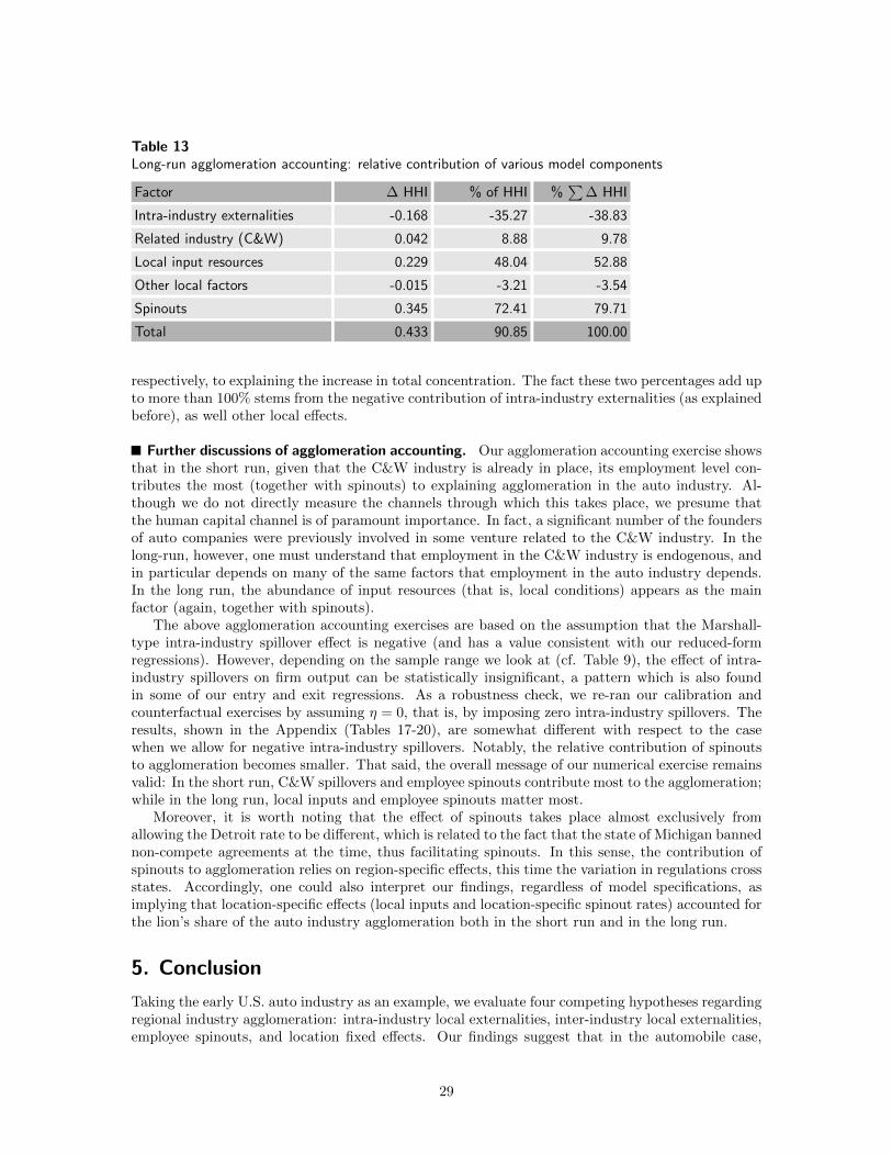
Table 13Long-run agglomeration accounting: relative contribution of various model components


∆ HHI

Intra-industry externalities -0.168 -35.27 -38.83



Other local factors -0.015 -3.21 -3.54

Spinouts 0.345 72.41 79.71

Total 0.433 90.85 100.00

respectively, to explaining the increase in total concentration. The fact these two percentages add upto more than 100% stems from the negative contribution of intra-industry externalities (as explainedbefore), as well other local effects.

Further discussions of agglomeration accounting. Our agglomeration accounting exercise showsthat in the short run, given that the C&W industry is already in place, its employment level con-tributes the most (together with spinouts) to explaining agglomeration in the auto industry. Al-though we do not directly measure the channels through which this takes place, we presume thatthe human capital channel is of paramount importance. In fact, a significant number of the foundersof auto companies were previously involved in some venture related to the C&W industry. In thelong-run, however, one must understand that employment in the C&W industry is endogenous, andin particular depends on many of the same factors that employment in the auto industry depends.In the long run, the abundance of input resources (that is, local conditions) appears as the mainfactor (again, together with spinouts).

The above agglomeration accounting exercises are based on the assumption that the Marshall-type intra-industry spillover effect is negative (and has a value consistent with our reduced-formregressions). However, depending on the sample range we look at (cf. Table 9), the effect of intra-industry spillovers on firm output can be statistically insignificant, a pattern which is also foundin some of our entry and exit regressions. As a robustness check, we re-ran our calibration andcounterfactual exercises by assuming η = 0, that is, by imposing zero intra-industry spillovers. Theresults, shown in the Appendix (Tables 17-20), are somewhat different with respect to the casewhen we allow for negative intra-industry spillovers. Notably, the relative contribution of spinoutsto agglomeration becomes smaller. That said, the overall message of our numerical exercise remainsvalid: In the short run, C&W spillovers and employee spinouts contribute most to the agglomeration;while in the long run, local inputs and employee spinouts matter most.

Moreover, it is worth noting that the effect of spinouts takes place almost exclusively fromallowing the Detroit rate to be different, which is related to the fact that the state of Michigan bannednon-compete agreements at the time, thus facilitating spinouts. In this sense, the contribution ofspinouts to agglomeration relies on region-specific effects, this time the variation in regulations crossstates. Accordingly, one could also interpret our findings, regardless of model specifications, asimplying that location-specific effects (local inputs and location-specific spinout rates) accounted forthe lion’s share of the auto industry agglomeration both in the short run and in the long run.

5. Conclusion

Taking the early U.S. auto industry as an example, we evaluate four competing hypotheses regardingregional industry agglomeration: intra-industry local externalities, inter-industry local externalities,employee spinouts, and location fixed effects. Our findings suggest that in the automobile case,

29

inter-industry local externalities (particularly from the carriage and wagon industry) and employeespinouts (particularly due to the high spinout rate in Detroit) play important roles. Local inputsalso explain differences in regional agglomeration. In the short run, this effect appears to be small.In the long run, however, once we account for the effect of local inputs on related industry location,it appears to play a much more important role. Finally, the presence of other firms in the sameindustry has a negligible or even negative effect on agglomeration.

Although we focus on the auto industry, we believe the patterns we find are likely found in otherindustries as well. For example, the relation we find between C&W and auto producers is similar tothat found between radio and TV producers (Klepper and Simons, 2000). Also, the relation betweenparent and spinout in autos is similar to the auto-tire industry clustered in Akron (Buenstorf andKlepper, 2009) and the IT industry clustered in Silicon Valley (Klepper, 2010). Finally, we also findlocation fixed effects on industry agglomeration that are consistent with many other manufacturingindustries (Ellison and Glaeser, 1997, 1999).

Our findings have an important policy implication: in order to boost regional development, pol-icymakers should evaluate location advantages (in terms of input resources and existing industries)before choosing to promote certain target industries. All too often, one finds countries, and regionswithin countries, eager to create “the next Silicon Valley” by means of a “cluster strategy” (essen-tially, a strategy that takes advantage of agglomeration and co-agglomeration economies). However,by failing to understand the dynamics of industry agglomeration, as well as the importance of loca-tion fixed effects, many of these initiatives fall very short of expectations.

Our study can be extended in several directions. First, while our paper focuses on the historicalevolution of auto industry, the analysis can be applied to other industries. In particular, it wouldbe interesting to explore similarities and differences with respect to more recent high-tech industries(both in terms of agglomeration patterns and in terms of driving forces). Second, due to datalimitation, we use entry and exit as proxy measures of firm performance. Provided richer databecomes available, future studies could use more direct measures of firm performance. Third, ourpaper points to possible channels through which local factors and externalities contribute to industryagglomeration. It would be interesting to study more precisely the nature and size of local spilloversthrough those channels. Finally, it would be useful to conduct cross-country comparisons of industryagglomeration in both advanced and developing economies. This will help us better understand thenature of increasing-return technologies and regional spillovers, which are important driving forcesfor economic growth, development, and international trade.

30

References

Arrow K.J. (1962), “The Economic Implications of Learning by Doing,” Review of Economic Studies 29,155–172.

Bailey, L.S. (1971), The American Car since 1775, Automobile Quarterly: New York.

Bloom, Nicholas, Mark Schankerman and John Van Reenen (2013), “Identifying Technology Spilloversand Product Market Rivalry,” Econometrica 81(4), 1347–1393.

Buenstorf, Guido, and Steven Klepper (2009), “Heritage and Agglomeration: The Akron Tyre ClusterRevisited,” The Economic Journal 119, 705–733.

Cabral, Luıs (2012), “Technology Uncertainty, Sunk Costs, and Industry Shakeout,” Industrial and Cor-porate Change 21, 539–552.

Cabral, Luıs, and Zhu Wang (2009), “Spinouts: Theory and Evidence from Early U.S. AutomobileIndustry,” Federal Reserve Bank of Kansas City Working Paper.

Chatterjee, Satyajit, and Esteban Rossi-Hansberg (2012), “Spin-Offs and the Market for Ideas,”International Economic Review 53 (1), 53–93.

Dumais, G., G. Ellison and E. L. Glaeser (2002), “Geographic Concentration As A Dynamic Process,”Review of Economics and Statistics 84 (2), 193–204.

Ellison, Glenn, and Edward L. Glaeser (1997), “Geographic Concentration in U.S. ManufacturingIndustries: A Dartboard Approach,” Journal of Political Economy 105 (5), 889–927.

Ellison, Glenn, and Edward L. Glaeser (1999), “The Geographic Concentration of Industry: DoesNatural Advantage Explain Agglomeration,” American Economic Review 89 (2), 311–316.

Ellison, G. and E.L. Glaeser and W. Kerr (2010), “What Causes Industry Agglomeration? Evidencefrom Coagglomeration Patterns,” American Economic Review 100 (3), 1195–1213.

Easterlin, Richard (1960), “Interregional Differences in Per Capita Income, Population, and Total In-come, 1840-1950,” in NBER conference volume Trends in the American Economy in the NineteenthCentury, UMI.

Franco, April, and Darren Filson (2006), “Spin-Outs: Knowledge Diffusion Through Employee Mo-bility,” Rand Journal of Economics 37, 841–860.

Franco, April, and Matthew Mitchell (2008), “Covenants not to Compete, Labor Mobility, andIndustry Dynamics,” Journal of Economics and Management Strategy 17(3), 581–606.

Glaeser, Edward L., Hedi D. Kallal, Jose A. Sheinkman, and Andrei Schleifer (1992), “Growthin Cities,” Journal of Political Economy 100, 1126–1152.

Gort, M., and S. Klepper (1982), “Time Paths in the Diffusion of Product Innovations,” EconomicJournal 92, 630–653.

Hanson, Gordon (2001), “Scale Economies and the Geographic Concentration of Industry,” Journal ofEconomic Geography 1 (3), 255–276.

Henderson, J.V. (1988), Urban Development: Theory, Fact, and Illusion, New York: Oxford UniversityPress.

Henderson, Vernon, Ari Kuncoro, and Matt Turner (1995), “Industrial Development in Cities,”Journal of Political Economy 103, 1067–1090.

31

Hopenhayn, Hugo (1992), “Entry, Exit, and Firm Dynamics in Long Run Equilibrium,” Econometrica 60(5), 1127–1150.

Jackson, John (1988), “Michigan,” in R. Scott Fosler (Ed), The New Role of American States, New York:Oxford University Press.

Jacobs, Jane (1969), The Economy of Cities, New York: Vintage Books.

Jovanovic, Boyan and Glenn M. MacDonald (1994), “The Life Cycle of a Competitive Industry,”Journal of Political Economy 102 (2), 322–347.

Kimes, Beverly R. (1996), Standard Catalog of American Cars, 1890–1942, third edition, Iola, WI: KrausePublications Inc.

Klepper, Steven (2002), “Firm Survival and the Evolution of Oligopoly,” RAND Journal of Economics33 (1), 37–61.

Klepper, Steven (2007), “Disagreements, Spinouts, and the Evolution of Detroit as the Capital of theU.S. Automobile Industry,” Management Science 53 (4), 616–631.

Klepper, Steven (2010), “The Origin and Growth of Industry Clusters: The Making of Silicon Valley andDetroit,” Journal of Urban Economics 67, 15–32.

Klepper, Steven and Kenneth Simons (2000), “Dominance by Birthright: Entry of Prior Radio Produc-ers and Competitive Ramifications in the U.S. Television Receiver Industry,” Strategic ManagementJournal 21(10–11), 997–1016.

Klepper, Steven and Kenneth Simons (2005), “Industry Shakeouts and Technological Change,” Inter-national Journal of Industrial Organization 23(1–2), 23–43.

Krugman, Paul (1991), Geography and Trade, Cambridge: MIT Press.

Leontief, Wassily W. (1951), The Structure of American Economy, 1919-1939, New York: Oxford Uni-versity Press.

Marshall, Alfred (1890), Principles of Economics, Macmillan, London.

Marx, Matt, Deborah Strumsky, and Lee Fleming (2009), “Mobility, Skills, and the Michigan Non-Compete Experiment,” Management Science 55(6), 875–889.

Romer, Paul M. (1986), “Increasing Returns and Long-run Growth,” Journal of Political Economy 94,1002–1037.

Rosental, Stuart and William Strange (2004), “Evidence on the Nature and Sources of AgglomerationEconomies,” Handbook of Urban and Regional Economics 4, 2119–2171.

Rubenstein, James M. (1992), The Changing US Auto Industry: A Geographical Analysis, New York:Routledge.

Smith, Philip H. (1970), Wheels within Wheels: A Short History of American Motor Car Manufacturing,New York: Funk and Wagnalls.

Thomas, Robert Paul (1977), An Analysis of the Pattern of Growth of the Automobile Industry 1895–1929,New York: Arno Press.

32

Appendix

A note on rescaling. This note proves that the industry equilibrium derived from our model isinvariant with respect to a rescaling of the model parameters, such as market size a and productiontechnology q(s), as long as firms’ average value of outside option σ is rescaled appropriately.

Given the demand function estimated in Section 4

log

(Q

pop

)= a− b log(p),

letting pop× exp(a) = Z, we can rewrite the market equilibrium condition in steady state as

log

∑s,j

q∗(s, p,mj)m(s, j)

= log(Z)− b log(p),

where q∗(s, p,mj) is the firm’s profit-maximizing output given the price p. Profit maximizationimplies

q∗(s, p,mj) = (αp)α

1−α

(exp(c1 s)m

ηj

) 11−α

.

Thus the market equilibrium price p∗(m,Z) is determined by

log(p∗) =log(Z)α

1−α + b− 1

α1−α + b

log

∑s,j

(α)α

1−α

(exp(c1 s)m

ηj

) 11−α

m(s, j)

.

We can then always compute an industry equilibrium which is invariant to the scale of Z as longas the firms’ outside options are subject to rescaling.39 Let the rescaled price

log(p) = log(p∗)− log(Z)α

1−α + b.

We can similarly rescale profit π(s, p), which is again Z dependent:

π(s, p∗,mj) =

(1

α− 1

)(αp∗)

11−α

(exp(c1 s)m

ηj

) 11−α

.

The profit function is given by π(s, p∗,mj) = Z1

α+b(1−α)π(s, p,mj).Finally, recall the firm value in steady state is given by

V C(s) = β

(π(s) + F

(V C(s)

)V C(s) +

(1− F

(V C(s)

))E(φ′|φ′ ≥ V C(s)

)).

Assuming φ is exponentially distributed (that is, F is exponential), we have

E(φ′|φ′ ≥ V C(s)

)= V C(s) + σ,

where σ is the mean of the firm’s outside option. Then we have

V C(s) = β

(π(s) +

(1− F

(V C(s)

))σ + V C(s)

)= β

(π(s) + exp

(− V C(s)/σ

)σ + V C(s)

).

39. We can also allow production technology q(s) to be rescaled, e.g. changing q∗(s, p) to λq∗(s, p) in the above

equation. We can then define a new scaling parameter Z = Z/λ and all the following proof goes through.

33

This implies that if the mean outside option also has a scale factor Z such that σ = Z1

α+b(1−α) σ,where σ is a constant, then we can go from

V C =(Z

1α+b(1−α) σ

)−1V C

to

V C(s) = β

(π(s)/σ + exp

(− V C(s)

)+ V C(s)

).

Hence, the firm’s rescaled value function, V C(s), is invariant with respect to Z. Because firm exit

rate is simply exp(−V C(s)), firm entry and exit rates in the steady state are invariant with respectto Z.

We have thus proved that industry equilibrium is invariant with respect to a rescaling of themodel parameters governing market size and production technology, as long as firms’ average valueof outside option is rescaled appropriately.

Proofs. The proofs of Propositions 1–3 follow.

Proof of Proposition 1: Note that an incumbent’s continuing decision is equivalent to a spinout’sentry decision. Given that π(s; j, p) is strictly increasing in s, continuous, and bounded, standarddynamic programming argument shows that V C(s; j, p) is continuous in s and strictly increasing ins for p > 0. Thus we know that for each period, F (V C(s; j, p)) is strictly increasing in s, given thesame location j.

Proof of Proposition 2: Note that for each period, all incumbents at location j have the sameprobability γj of having a potential spinout. Also, we show above that an incumbent (a potentialspinout) is more likely to survive (enter) if it belongs to a higher capability family. Thus, a higher-capability family has a bigger family size on average, given that (1 + γj)χs,j increases in s.

Proof of Proposition 3: The stationary distribution is defined by m∗j = m∗j (1 + γj)χ∗j + njµj , so

m∗j =nj

1−(1+γj)χ∗jµj . The distribution of spinout firms is m∗jχ

∗j =

njχ∗j

1−(1+γ)χ∗jµj . Since χ∗j is strictly

increasing in s, the capability distribution of spinout firms strictly dominates that of de novo firms,which is µj .

Additional regression results (Tables 14, 15, 16).

34

Table 14Spinout location and spinout performance.Logit models of firm exit, 1900-1935. Dependent variable: firm exit at time t


Firm age -0.069***(0.010)

-0.056***(0.009)

-0.077***(0.010)

-0.064***(0.010)

Dealio -0.458***(0.107)

-0.454***(0.105)

-0.479***(0.108)

-0.471***(0.105)

Spinout -0.432***(0.156)

-0.240(0.158)

-0.421***(0.159)

-0.232(0.160)


0.014*(0.007)

Local family size -0.102**(0.042)

-0.113**(0.048)

Non-local family size -0.053(0.074)

-0.092(0.084)

Center top 0.020(0.033)

0.022(0.034)

Local family top -0.448***(0.097)

-0.482***(0.106)

Non-local family top -0.083(0.125)

-0.135(0.149)


0.072(0.058)

0.133**(0.066)

0.155**(0.067)


0.185(0.165)

0.282*(0.165)

0.299*(0.162)


0.324(0.298)

0.175(0.317)

0.124(0.312)


-0.160(0.139)

-0.263*(0.150)

-0.309**(0.144)


0.032(0.045)

0.011(0.049)

0.021(0.049)


-0.093(0.112)

-0.114(0.112)

-0.125(0.114)

St Louis 0.161(0.317)

0.180(0.322)

0.033(0.316)

0.090(0.315)

Chicago -0.275(0.223)

-0.128(0.193)

-0.377(0.241)

-0.130(0.195)

Indianapolis -0.551**(0.267)

-0.415*(0.228)

-0.671**(0.291)

-0.430*(0.234)

Detroit -0.654**(0.301)

-0.372(0.484)

-0.929**(0.362)

-0.444(0.501)

Rochester -0.373(0.286)

-0.316(0.273)

-0.442(0.286)

-0.327(0.268)


0.106(0.202)

-0.112(0.233)

0.133(0.202)

Year or year dummies 0.023(0.015)

0.012(0.014)

yeardummies

yeardummies

Constant -46.127(29.746)

-25.398(26.749)

-0.365(1.943)

-0.041(1.913)

Observations 3,573 3,573 3,537 3,537

Notes: Center size, Local family size, Non-local family size, Center top, Local family top and Non-local familytop one-year lagged; Log auto employment is calculated by taking the logarithm of three-year lagged averageof auto employment in each location.

Robust standard errors clustered by firm. Star levels: 10, 5 and 1%.

35

Table 15Logit models of spinout firm exit, 1900-1935. Dependent variable: firm exit at time t


Firm age -0.073***(0.025)

-0.071***(0.024)

-0.075***(0.027)

-0.074***(0.027)

Center size 0.038**(0.017)

0.043*(0.025)

Family size -0.058(0.044)

-0.081(0.053)

Center top 0.143(0.107)

0.239**(0.121)

Family top -0.209***(0.076)

-0.208***(0.080)

Log auto employment -0.301(0.333)

-0.162(0.323)

-1.556***(0.552)

-1.860***(0.708)

Log population 1900 -2.222(2.022)

-1.039(1.854)

-6.529**(2.895)

-7.837**(3.898)


-1.225(2.025)

-3.310(3.171)

-5.253(4.571)

Log C&W employment 1905 0.250(0.825)

0.113(0.787)

1.282(1.003)

1.539(1.016)


0.238(0.485)

0.293(0.608)

0.427(0.583)


0.393(1.729)

3.979(2.455)

4.893(3.164)

St Louis -0.678(0.973)

-0.326(0.785)

-0.639(1.194)

0.184(1.138)

Chicago -1.246*(0.745)

-0.781(0.690)

-1.722*(0.970)

-1.294(0.836)

Indianapolis -1.478***(0.571)

-0.829*(0.430)

-2.027***(0.764)

-1.369**(0.572)

Detroit -2.491***(0.939)

-2.605(1.726)

-2.145*(1.189)

-3.674*(1.906)

Rochester -0.753(0.494)

-0.901*(0.488)

-0.396(0.609)

-0.434(0.569)


0.059(0.570)

-0.268(0.759)

-0.113(0.645)

Year 0.129**(0.064)

0.079(0.057)

dummies dummies

Constant -240.071**(122.213)

-146.257(109.043)

6.269(9.670)

10.966(10.993)

Observations 720 720 658 658


36

Table 16Logit models of non-spinout firm exit, 1900-1935. Dependent variable: firm exit at time t


Firm age -0.064***(0.011)

-0.039***(0.012)

-0.079***(0.013)

-0.055***(0.014)

De Alio -0.447***(0.108)

-0.441***(0.105)

-0.470***(0.108)

-0.459***(0.105)


0.010(0.008)

Family size -0.242(0.184)

-0.226(0.185)

Center top 0.005(0.037)

0.008(0.037)

Family top -1.072***(0.251)

-1.089***(0.258)


0.076(0.060)

0.174**(0.070)

0.196***(0.071)


0.212(0.170)

0.335*(0.174)

0.307*(0.166)


0.390(0.323)

0.018(0.331)

0.023(0.336)


-0.155(0.142)

-0.375**(0.159)

-0.356**(0.146)


0.037(0.048)

0.004(0.052)

0.019(0.053)


-0.117(0.115)

-0.093(0.116)

-0.136(0.118)

St Louis 0.290(0.354)

0.231(0.370)

0.198(0.345)

0.170(0.361)

Chicago -0.147(0.244)

-0.059(0.211)

-0.220(0.265)

-0.046(0.214)

Indianapolis -0.447(0.294)

-0.425*(0.254)

-0.555*(0.324)

-0.464*(0.269)

Detroit -0.439(0.342)

-0.121(0.544)

-0.697*(0.395)

-0.237(0.542)

Rochester -0.339(0.303)

-0.279(0.288)

-0.374(0.308)

-0.264(0.291)


0.149(0.219)

-0.055(0.254)

0.214(0.219)

Year 0.016(0.016)

0.005(0.015)

dummies dummies

Constant -32.965(31.472)

-10.883(29.284)

0.469(2.091)

0.805(2.087)

Observations 2,853 2,853 2,832 2,832


37

Model Calibration and Simulations without Intra-industry Spillovers (η = 0)

Table 17Short-run decomposition. Model fit and five counterfactuals: 1. Uniform C&W employment levels; 2.Uniform input resources; 3. Uniform other factors (population, income, shipbuilding, location dummies,etc); 4. No spinout; 5. No Detroit-specific spinout rate

Counterfactuals

Data Model 1 2 3 4 5

Output share

Chicago 0.060 0.034 0.037 0.027 0.036 0.059 0.058

Detroit 0.670 0.675 0.295 0.489 0.492 0.369 0.371

New York 0.140 0.090 0.055 0.032 0.399 0.166 0.164

Indianapolis 0.070 0.101 0.040 0.186 0.016 0.212 0.215

St Louis 0.010 0.008 0.021 0.018 0.007 0.013 0.013

Others 0.060 0.092 0.553 0.249 0.051 0.180 0.180

HHI 0.477 0.476 0.101 0.277 0.402 0.213 0.215

Prediction MSE 0.001 0.065 0.016 0.017 0.021 0.021

Exit rate

Non-Detroit 0.150 0.146 0.145 0.145 0.147 0.142 0.142

Detroit 0.130 0.135 0.142 0.134 0.136 0.136 0.137

Additional moments

Average regional spinout rate 0.030 0.038 0.033 0.032 0.034 0 0.017

Detroit top spinout rate 0.079 0.073 0.074 0.073 0.073 0 0.019

Table 18Short-run agglomeration accounting: relative contribution of various model components


∆ HHI

Intra-industry externalities 0.000 0.00 0.00




Spinouts 0.263 55.25 28.87

Total 0.911 191.39 100.00

38

Table 19Long-run decomposition. Model fit and five counterfactuals: 1. Uniform C&W employment shocks(which are not explained by local conditions); 2. Uniform input resources; 3. Uniform other factors(population, income, shipbuilding, location dummies, etc); 4. No spinout; 5. No Detroit-specificspinout rate

Counterfactuals

Data Model 1 2 3 4 5

Output share

Chicago 0.060 0.034 0.044 0.020 0.037 0.059 0.058

Detroit 0.670 0.675 0.524 0.268 0.644 0.369 0.371

New York 0.140 0.090 0.309 0.016 0.202 0.166 0.164

Indianapolis 0.070 0.101 0.012 0.106 0.039 0.212 0.215

St Louis 0.010 0.008 0.007 0.039 0.007 0.013 0.013

Others 0.060 0.092 0.104 0.550 0.072 0.180 0.180

HHI 0.477 0.476 0.373 0.093 0.458 0.213 0.215

Prediction MSE 0.001 0.010 0.070 0.001 0.021 0.021

Exit rate

Non-Detroit 0.150 0.146 0.147 0.143 0.147 0.142 0.142

Detroit 0.130 0.135 0.137 0.137 0.131 0.136 0.137

Additional moments

Average regional spinout rate 0.030 0.038 0.036 0.027 0.034 0 0.017

Detroit top spinout rate 0.079 0.073 0.073 0.074 0.073 0 0.019

Table 20Long-run agglomeration accounting: relative contribution of various model components


∆ HHI

Intra-industry externalities 0.000 0.00 0.00




Spinouts 0.263 55.25 34.29

Total 0.767 161.13 100.00

39

Working Paper Series - Federal Reserve Bank of Richmond · mobile case, inter-industry local...

Documents

Transcript of Working Paper Series - Federal Reserve Bank of Richmond · mobile case, inter-industry local...