Working Paper Series

This paper can be downloaded without charge from: http://www.richmondfed.org/publications/

The Time-Varying Beveridge Curve∗

Luca BenatiUniversity of Bern†

Thomas A. LubikFederal Reserve Bank

of Richmond‡

August 2013

Working Paper No. 13-12

Abstract

We use a Bayesian time-varying parameter structural VAR with stochastic volatilityto investigate changes in both the reduced-form relationship between vacancies and theunemployment rate, and in their relationship conditional on permanent and transitoryoutput shocks, in the post-WWII United States. Evidence points towards similaritiesand differences between the Great Recession and the Volcker disinflation, and wide-spread time variation along two key dimensions. First, the slope of the Beveridge curveexhibits a large extent of variation from the mid-1960s on. It is also notably pro-cyclical,whereby the gain is positively correlated with the transitory component of output. Theevolution of the slope of the Beveridge curve during the Great Recession is very sim-ilar to its evolution during the Volcker recession in terms of both its magnitude andits time profile. Second, both the Great Inflation episode and the subsequent Volckerdisinflation are characterized by a significantly larger negative correlation between thereduced-form innovations to vacancies and the unemployment rate than the rest of thesample period. Those years also exhibit a greater cross-spectral coherence between thetwo series at business-cycle frequencies. This suggests that they are driven by commonshocks.

JEL Classification: C11, C32, E20, E24,Keywords: Bayesian VARs; stochastic volatility; time-varying parameters;

Great Recession; Great Inflation; long-run restrictions

∗The views in this paper are those of the authors and should not be interpreted as those of the FederalReserve Bank of Richmond, the Board of Governors, or the Federal Reserve System. We are grateful toparticipants at the Applied Time Series Econometrics Workshop at the Federal Reserve Bank of St. Louisand the Midwest Macroeconomics Meetings at the University of Colorado Boulder for useful comments andsuggestions.†Department of Economics, University of Bern, Schanzeneckstrasse 1, CH-3001 Bern, Switzerland. Email:

luca.benati@vwi.unibe.ch‡Research Department, Federal Reserve Bank of Richmond, 701 E Byrd Street, Richmond, VA 23218,

USA. E-mail: Thomas.Lubik@rich.frb.org

1

1 Introduction

The Beveridge curve describes the relationship between the unemployment rate and open

positions, that is, vacancies, in the labor market. Plotting the former against the latter in a

scatter diagram reveals a downward-sloping relationship that appears to be clustered around

a concave curve (see Figure 1). The curve reflects the highly negative correlation between

unemployment and vacancies that is a hallmark of labor markets in market economies.

Empirical work on the Beveridge curve has explored the relationship between vacancies

and the unemployment rate under the maintained assumption that it can be regarded, as

a first approximation, as time-invariant. The behavior of the two series during the Great

Recession, with the unemployment rate seemingly stuck at high levels, even in the presence

of a vacancy rate that has been progressively improving, has, however, raised doubts about

the validity of the assumption of time-invariance. This suggests exploring the relationship

between the two series allowing for the possibility that it may have evolved over time.

Our paper builds directly on the seminal contribution of Blanchard and Diamond (1989).

These authors reintroduced the concept of the Beveridge curve as one of the key relation-

ships in macroeconomic data. They conducted a vector autoregression (VAR) analysis of

unemployment, vacancies, and the labor force in order to identify the driving forces behind

movements in the Beveridge curve. We build upon their analysis by identifying both per-

manent and transitory structural shocks in a time-varying VAR context. By doing so, we

are able to trace out the sources of movements, shifts, and tilts in the Beveridge curve over

time.

The theoretical background for our study, and one that we use for identifying the struc-

tural shocks, is the simple search and matching approach to modeling labor markets (see

Shimer, 2005). The Beveridge curve encapsulates the logic of this model. In times of

economic expansions, unemployment is low and vacancies, that is, open positions offered

by firms, are plentiful. Firms want to expand their workforce, but they are unable to do

so since the pool of potential employees (that is, the unemployed) is small. As economic

conditions slow down and demand slackens, firms post fewer vacancies and unemployment

rises, consistent with a downward move along the Beveridge curve. At the trough of the

business cycle, firms may have expectations of a future uptick in demand and start posting

open positions. This decision is amplified by the large pool of unemployed, which guar-

antees firms high chances of finding suitable candidates and thus outweighs the incurred

search costs. As the economy improves, unemployment falls and vacancy postings rise in

2

an upward move along the Beveridge curve.

We approach the Beveridge curve empirically by specifying a time-varying parameter

VAR with stochastic volatility. Our choice is informed by the observation that there are

patterns in the Beveridge-curve relationship that are ill described by a linear framework.

Specifically, the data suggest that the slope of the Beveridge curve is different for each

business cycle episode, that the curve shifts over time, and that the pattern of driving

forces change in a nonlinear fashion as well. Naturally, nonlinearity can take many forms,

as do the framework to capture this. We utilize a time-varying parameter framework since

it is a reasonably straightforward extension of linear VARs. Moreover, and perhaps more

importantly, it can capture and approximate a wide range of underlying nonlinear behavior.

To this point, we will introduce time variation in a nonlinear theoretical model of the labor

market in order to relate it to the results from the VAR.

Our empirical analysis starts by documenting the presence of time variation in the

relationship between vacancies and the unemployment rate by means of Stock and Watson’s

(1996, 1998) time-varying parameter median-unbiased estimation, which allows us to test

for the presence of random-walk time variation in the data. Having detected evidence of

time variation in the bivariate relationship between vacancies and the unemployment rate,

we then use a Bayesian time-varying parameter structural VAR with stochastic volatility to

characterize changes over time in the relationship. Evidence points towards both similarities

and differences between the Great Recession and the Volcker disinflation, and widespread

time variation along two key dimensions.

First, the slope of the Beveridge curve, which we capture by the average gain of the

unemployment rate onto vacancies at business cycle frequencies is strongly negatively cor-

related with the Congressional Budget Offi ce’s (CBO) estimate of the output gap. The

evolution of the slope of the Beveridge curve during the Great Recession is very similar

to its evolution during the Volcker recession in terms of both its magnitude and its time

profile. This suggests that the seemingly anomalous behavior of the Beveridge curve during

the Great Recession, which has attracted much attention in the literature, may not have

been that unusual. Second, both the Great Inflation episode and the subsequent Volcker

disinflation, are characterized by a significantly larger (in absolute value) negative correla-

tion between the reduced-form innovations to vacancies and the unemployment rate than

the rest of the sample period. These years also show a greater cross-spectral coherence

between the two series at business-cycle frequencies. This suggests that they are driven, to

a larger extent than the rest of the sample, by common shocks.

3

Having characterized changes over time in the relationship between vacancies and the

unemployment rate, we then proceed to interpret these stylized facts based on an estimated

search and matching model. Specifically, we explore within a simple theoretical model how

changes in individual parameter values affect the relationship between vacancies and the

unemployment rate in order to gauge the origin of the variation in the Beveridge relationship.

The paper is organized as follows. The next section presents preliminary evidence on the

presence of (random-walk) time variation in the bivariate relationship between the vacancy

rate and the unemployment rate. Section 3 describes the Bayesian methodology we use

to estimate the time-varying parameter VAR with stochastic volatility, whereas Section

4 discusses the evidence of changes over time in the Beveridge relationship. Section 5

details our structural identification procedure based on insights from a simple search and

matching model, where we discuss implementation of both long-run and sign restrictions.

We present the results of the structural identification procedure in Section 6. We also explore

how changes in individual structural parameters of the search and matching model map

into corresponding changes in the relationship between vacancies and the unemployment

rate. Section 7 concludes. An appendix contains a detailed description of the econometric

methods and the theoretical model we use for identification purposes.

2 Searching for Time Variation in the Beveridge Relation-ship

Figure 1 presents a time series plot of the unemployment rate and vacancies from 1949 to

2011. The negative relationship between the two series is readily apparent. At the peak

of the business cycle unemployment is low and vacancies are high. Over the course of a

downturn the former rises and the latter declines as fewer and fewer workers are employed

and firms have fewer and fewer open positions. Volatility and serial correlation of both

series appear of similar magnitude. The second panel in Figure 1 depicts the same series in

a scatter plot of vacancies against unemployment, resulting in the well-known downward-

sloping relationship that has come to be known as the Beveridge curve. In the graph, we

plot individual Beveridge curves for each NBER business cycle. Each episode starts at

the business cycle peak and ends with the period before the next peak. Visual inspection

reveals two observations. First, all curves are downward-sloping, but with different slopes.

Second, there is substantial lateral movement in the individual Beveridge curves, ranging

from the innermost cycle, the 1953-1957 episode, to the outermost, 1982-1990. We take

these observations as motivating evidence that the relationship between unemployment

4

and vacancies exhibits substantial variation over time, which a focus on a single aggregate

Beveridge curve obscures.

Time variation in data and in theoretical models can take many forms, from continuous

variations in unit-root time-varying parameter models to discrete parameter shifts such as

regime-switching. We regard both discrete and continuous changes as a priori plausible. In

this paper, we focus on the latter. We thus provide evidence of time variation in the bivariate

relationship between vacancies and unemployment. We apply the methodology developed

by Stock and Watson (1996, 1998) to test for the presence of random-walk time-variation

in the two-equation VAR representation for the two variables.1

The regression model we consider is:

xt = µ+ α(L)Vt−1 + β(L)Ut−1 + εt ≡ θ′Zt + εt, (1)

where xt = Vt, Ut, with Vt and Ut being the vacancy rate and the unemployment rate,

respectively. α(L) and β(L) are lag polynomials; θ = [µ, α(L), β(L)]′ and Zt = [1, Vt−1,

..., Ut−p]′. We select the lag order as the maximum of the lag orders individually chosen

by the Akaike, Schwartz, and Hannan-Quinn criteria. Letting θt = [µt, αt(L), βt(L)]′, the

time-varying parameter version of (1) is given by:

xt = θ′tZt + εt, (2)

θt = θt−1 + ηt, (3)

with ηt ∼ iid N (04p+1, λ2σ2Q), where 04p+1 is a (4p + 1)-dimensional vector of zeros.

σ2 is the variance of εt, Q a covariance matrix, and E[ηtεt] = 0. Following Stock and

Watson (1996, 1998), we set Q = [E(ZtZ′t)]−1. Under this normalization, the coeffi cients

on the transformed regressors, [E(ZtZ′t)]−1/2Zt, evolve according to a (4p+ 1)-dimensional

standard random walk, where λ2 is the ratio between the variance of each transformed

innovation and the variance of εt. We estimate the matrix Q as Q =[T−1

∑Tt=1 ztz

′t

]−1.

We estimate the specification (1) by OLS, from which we obtain an estimate of the

innovation variance, σ2. We then perform an exp- and a sup-Wald joint test for a single

unknown break in µ and in the sums of the α’s and β’s, using either the Newey and West

1From an empirical perspective, we prefer their methodology over, for instance, structural break tests forreasons of robustness to uncertainty regarding the specific form of time-variation present in the data. Whiletime-varying parameter models can successfully track processes subject to structural breaks, Cogley andSargent (2005) and Benati (2007) show that break tests possess low power when the true data-generatingprocess (DGP) is characterized by random walk time variation. Generally speaking, break tests performwell if the DGP is subject to discrete structural breaks, while time-varying parameter models perform wellunder both scenarios.

5

(1987) or the Andrews (1991) HAC covariance matrix estimator to control for possible

autocorrelation and/or heteroskedasticity in the residuals. Following Stock and Watson

(1996), we compute the empirical distribution of the test statistic by considering a 100-

point grid of values for λ over the interval [0, 0.1]. For each element of the grid we compute

the corresponding estimate of the covariance matrix of ηt as Qj=λ2j σ2Q; conditional on Qj

we simulate the model (2)-(3) 10,000 times, drawing the pseudo innovations from pseudo-

random iid N(0, σ2). We compute the median-unbiased estimate of λ as that particular

value for which the median of the simulated empirical distribution of the test is closest to the

test statistic previously computed based on the actual data. Finally, we compute the p-value

based on the empirical distribution of the test conditional on λj = 0, which we compute

based on Benati’s (2007) extension of the Stock and Watson (1996, 1998) methodology.

We report the estimation results in Table 1. We find strong evidence of random-walk

time variation in the equation for the vacancy rate. The p-values for the null of no time

variation range from 0.0028 to 0.0195, depending on the specific test statistic. The median-

unbiased estimates of λ are comparatively large, between 0.0235 and 0.0327. On the other

hand, the corresponding p-values for the unemployment rate are much larger, ranging from

0.1661 to 0.2594, which suggests time-invariance. However, the densities of the median-

unbiased estimates of λ in Figure 2 paint a more complex picture. A substantial fraction

of the probability mass are clearly above zero, whereas median-unbiased estimates of λ

range between 0.0122 and 0.0153. Although, strictly speaking, the null hypothesis of no

time variation cannot be rejected at conventional significance levels in a frequentist sense,

the evidence reported in Figure 2 suggests more caution. In what follows, we will proceed

under the assumption that both equations feature random-walk time variation. We now

investigate the changing relationship between the vacancy rate and the unemployment rate

based on a Bayesian time-varying parameter VAR.

3 A Bayesian Time-Varying Parameter VAR with StochasticVolatility

We define the data vector Yt ≡ [∆yt, Vt, Ut]′, where ∆yt is real GDP growth, computed as

the log-difference of real GDP; Vt is the vacancy rate based the Conference Board’s Help-

Wanted Index and Barnichon’s (2010) extension; and Ut is the unemployment rate. The

data are all quarterly. The vacancies and unemployment series are both normalized by the

labor force, seasonally adjusted, and converted from the original monthly series by simple

averaging. The overall sample period is 1951Q1-2011Q4. We use the first 15 years of data

6

to compute the Bayesian priors, which makes the effective sample period 1965Q1-2011Q4.

Appendix A contains a complete description of the data and of their sources.

We specify the time-varying parameter V AR(p) model:

Yt = B0,t +B1,tYt−1 + ...+Bp,tYt−p + εt ≡ X′tθt + εt. (4)

The notation is standard. As is customary in the literature on Bayesian time-varying

parameter VARs, we set the lag order to p = 2. The time-varying lag coeffi cients, collected

in the vector θt, are postulated to evolve according to:

p(θt | θt−1, Q) = I(θt) f(θt | θt−1, Q), (5)

where I(θt) is an indicator function that rejects unstable draws and thereby enforces sta-

tionarity on the VAR. The transition f(θt | θt−1, Q) is given by:

θt = θt−1 + ηt, (6)

with ηt ∼ iid N (0, Q).

We assume that the reduced-form innovations εt in (4) are normally distributed with

zero mean, where we factor the time-varying covariance matrix Ωt as:

V ar(εt) ≡ Ωt = A−1t Ht(A−1t )′. (7)

The time-varying matrices Ht and At are defined as:

Ht ≡

h1,t 0 00 h2,t 00 0 h3,t

, At ≡

1 0 0α21,t 1 0α31,t α32,t 1

. (8)

We assume that the hi,t evolve as geometric random walks:

lnhi,t = lnhi,t−1 + νi,t, i = 1, 2, 3. (9)

For future reference, we define ht ≡ [h1,t, h2,t, h3,t]′ and νt = [ν1,t, ν2,t, ν3,t]′, with νt ∼iid N (0, Z) and Z diagonal. We assume, as in Primiceri (2005), that the non-zero and

non-unity elements of the matrix At, which we collect in the vector αt ≡ [α21,t, α31,t, α32,t]′,

evolve as random walks:

αt = αt−1 + τ t , (10)

where τ t ∼ iid N (0, S). Finally, we assume that the innovations vector [u′t, η′t, τ′t, ν

′t]′ is

distributed as: utηtτ tνt

∼ N (0, V ) , with V =

I3 0 0 00 Q 0 00 0 S 00 0 0 Z

, (11)

7

where ut is such that εt ≡ A−1t H12t ut.

We follow the literature in imposing a block-diagonal structure for V , mainly for par-

simony, since the model is already quite heavily parameterized. Allowing for a completely

generic correlation structure among different sources of uncertainty would also preclude any

structural interpretation of the innovations. Finally, following Primiceri (2005) we adopt

the additional simplifying assumption of a block-diagonal structure for S:

S ≡ V ar (τ t) = V ar (τ t) =

[S1 01×2

02×1 S2

], (12)

with S1 ≡ V ar (τ21,t), and S2 ≡ V ar ([τ31,t, τ32,t]′). This implies that the non-zero

and non-one elements of At, which belong to different rows, evolve independently. This

assumption simplifies inference substantially, since it allows Gibbs sampling on the non-

zero and non-one elements of At equation by equation. We estimate (4)-(12) using standard

Bayesian methods. Appendix B discusses our choices for the priors, and the Markov-Chain

Monte Carlo algorithm we use to simulate the posterior distribution of the hyperparameters

and the states conditional on the data.

4 Reduced-Form Evidence

Figure 3 presents the first set of reduced-form results. It shows statistics of the estimated

time-varying innovations in the VAR (4). The first panel depicts the median posterior es-

timate of the correlation coeffi cient of the innovations to vacancies and the unemployment

rate and associated 68% and 90% coverage regions. The plot shows substantial time varia-

tion in this statistic. From the late 1960s to the early 1980s the correlation strengthens from

−0.4 to −0.85 before rising (in absolute value) to a low of −0.25. Over the course of the last

decade, the correlation has strengthened again, settling close to the average median value

of −0.55. This suggests that the unemployment-vacancy correlation strengthens during pe-

riods of broad downturns and high volatility, whereas it weakens in general upswings with

low economic turbulence. The evidence over the last decade also supports the impression

that the U.S. economy is in a period of a prolonged downswing.2

The impression of substantial time variation is strongly supported by the second panel,

which shows the fraction of draws from the posterior distribution for which the correlation

coeffi cient is greater than the average median value over the sample. The fraction of draws

2We also note that at the same time the coverage regions are tightly clustered around the median estimateduring the period of highest instability, namely the last 1970s and the Volcker disinflation, whereas they aremore spread out in the beginning and towards the end of the sample.

8

sinks toward zero at the end of the Volcker disinflation, while it oscillates for much of the

Great Moderation between 0.6 and 0.9. Similarly to the results in the first panel, the period

since the beginning of the financial crisis in August 2007 is characterized by a substantial

decrease in the fraction of draws.

In the third panel of Figure 3, we highlight the ratio of the estimated standard devi-

ations of the unemployment and vacancy innovations. The graph shows substantial time

variation in this ratio, although overall both innovation variances are of roughly equal size.

While the innovation variance of the vacancy rate appears overall dominant, unemployment

innovations play a relatively larger role at the end of the Great Inflation, the Volcker disin-

flation, and the Great Recession. All of these are periods during which the unemployment

rate shot up sharply. This suggests a dominant role of specific shocks, namely those tied

closely to reduced-form innovations to the unemployment rate, at the onset of an economic

downturn. We attempt to identify the sources for this behavior in the following section.

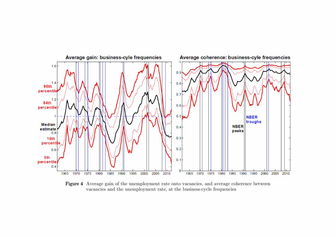
We now narrow our focus to the behavior of unemployment and vacancies at the business-

cycle frequencies between six quarters and eight years. We report these results using statis-

tics from the frequency domain. Figure 4 shows median posterior estimates (and associated

coverage regions) of the average cross-spectral gain and coherence between the two vari-

ables. The gain of a variable xt onto another variable yt at the frequency ω is defined as

the absolute value of the OLS-coeffi cient in the regression of yt on xt at that frequency,

whereas the coherence is the R2 in that regression. Consequently, the gain has a natural

interpretation in terms of the slope of the Beveridge curve, while the coherence measures

the fraction of the vacancy-rate’s variance at given frequencies that is accounted for by

the variation in the unemployment rate. We find it convenient to express time variation

in the Beveridge curve in terms of the frequency domain since it allows us to isolate the

fluctuations of interest, namely policy-relevant business cycles, and therefore abstract from

secular movements.

Overall, evidence of time variation is significantly stronger for the gain than for the co-

herence. The coherence between the two series appears to have remained broadly unchanged

since the second half of the 1960s, except for a brief run-up during the Great Inflation of

the 1970s, culminating in the tight posterior distribution during the Volcker disinflation of

the early 1980s. Moreover, average coherence is always above 0.8, with 0.9 contained in

the 68% coverage region. The high explanatory power of one variable for the other at the

business cycle frequencies thus suggests that unemployment and vacancies are driven by a

set of common shocks over the sample period.

9

The gain is large during the same periods in which the relative innovation variance of

reduced-form shocks to the unemployment rate is large, namely during the first oil shock,

the Volcker recession, and the Great Recession; that is, during these recessionary episodes

movements in the unemployment rate are relatively larger than those in the vacancy rate.

This points towards a flattening of the Beveridge curve in downturns, when small movements

in vacancies are accompanied by large movements in unemployment. Time variation in the

gain thus captures the shifts and tilts in the individual Beveridge curves highlighted in

Figure 1 in one simple statistic.

As a side note, our evidence does not indicate fundamental differences between the

Volcker disinflation and the Great Recession, that is, between the two deepest recessions in

the post-war era. This is especially apparent from the estimated gain in Figure 4, which

shows a similar time profile during both episodes. The relationship between vacancies and

unemployment, although clearly different from the years leading up to the financial crisis,

is broadly in line with that of the early 1980s.

We can now summarize our findings from the reduced-form evidence as follows. The

correlation pattern between unemployment and vacancies shows a significant degree of time

variation. It strengthens during downturns and weakens in upswings. This is consistent

with the idea that over the course of a business cycle, as the economy shifts from a peak

to a trough, labor market equilibrium moves downward along the Beveridge curve. This

movement creates a tight negative relationship between unemployment and vacancies. As

the economy recovers, however, vacancies start rising without much movement in unemploy-

ment. Hence, the correlation weakens. The economy thus goes off the existing Beveridge

curve, in the manner of a counter-clockwise loop, as identified by Blanchard and Diamond

(1989), or it moves to a new Beveridge curve, as suggested by the recent literature on

mismatch, e.g. Furlanetto and Groshenny (2012), Lubik (2012), and Sahin et al. (2012).

Evidence from the frequency domain suggests that the same shocks underlie movements

in the labor market, but that over the course of the business cycle shocks change in their

importance. During recessions movements in unemployment dominate, while in upswings

vacancies play a more important role. We now try to identify the structural factors deter-

mining this reduced-form behavior.

5 Identification

A key focus of our analysis is to identify the underlying sources of the movements in the

Beveridge curve. In order to do so we need to identify the structural shocks behind the

10

behavior of unemployment and vacancies. Our data set contains a nonstationary variable,

GDP, and two stationary variables, namely the unemployment and vacancy rates. This

allows us to identify one permanent and two transitory shocks from the reduced-form in-

novation covariance matrix. While the permanent shock has no effect on the two labor

market variables in the long run, it can still lead to persistent movements in these variables,

and thus in the Beveridge curve, in the short to medium run.3 More specifically, we are

interested in which shocks can be tied to the changing slope and the shifts in the Beveridge

curve. We let our identification strategy be guided by the implications of the simple search

and matching model, which offers predictions for the effects of permanent and transitory

productivity shocks as well as for other transitory labor market disturbances.

5.1 A Simple Theoretical Framework

We organize the interpretation of our empirical findings around the predictions of the stan-

dard search and matching model of the model labor market as described in Shimer (2005).

The model is a data-generating process for unemployment and vacancies that is driven

by a variety of fundamental shocks. The specific model is taken from Lubik (2012). The

specification and derivation is described in more detail in the appendix.

The model can be reduced to three key equations that will guide our thinking about the

empirics. The first equation describes the law of motion for employment:

Nt+1 = (1− ρt+1)[Nt +mtU

ξt V

1−ξt

]. (13)

The stock of existing workers Nt is augmented by new hires mtUξt V

1−ξt , which are the re-

sult of a matching process between open positions Vt and job seekers Ut via the matching

function. The matching process is subject to exogenous variation in the match effi ciency

mt, which affects the size of the workforce with a one-period lag. Similarly, employment

is subject to exogenous variations in the separation rate ρt, which affects employment con-

temporaneously. It is this timing convention that gives rise to an identifying restriction.

The second equation is the job-creation condition, which describes the optimal vacancy

posting decision by a firm:

κtmt

θξt = βEt(1− ρt+1)[(1− η) (At+1 − bt+1)− ηκt+1θt+1 +

κt+1mt+1

θξt+1

]. (14)

3While this rules out strict hysteresis effects, in the sense that temporary shocks can have permanenteffects, it can still lead to behavior that looks over typical sample periods as hysteresis-induced. Moreover,the empircial evidence concerning hysteresis is decidedly mixed.

11

θt = Vt/Ut is labor market tightness and a crucial statistic in the search and matching

model. Effective vacancy creation costs κtmtθξt are increasing in tightness since firms have to

compete with other firm’s hiring efforts given the size of the applicant pool. Hiring costs

are subject to exogenous variations in the component κt and have to be balanced against

the expected benefits, namely the right-hand side of the above equation. This consists of

surplus of a worker’s marginal product At over his outside options (unemployment benefits

bt), net of a hold-up term, ηκtθt, accruing to workers and extracted from the firm on account

of the latter’s costly participation in the labor market, and the firm’s implicit future cost

savings κtmtθξt when having already hired someone. η is a parameter indicating the strength of

worker’s bargaining power. Finally, production is assumed to be linear in employment, but

subject to both permanent and temporary productivity shocks, APt and ATt , respectively:

Yt = AtNt =(APt A

Tt

)Nt. (15)

The permanent shock is a pure random walk, while the temporary shock is serially correlated

but stationary.

Figure 5 depicts the theoretical impulse response functions of the unemployment and

vacancy rate to each of the shocks. We can categorize the shocks in two groups, namely

into shocks that move unemployment and vacancies in the same direction, and those that

imply opposite movements of these variables. This classification underlies the identification

by sign restrictions that we use later on. Both productivity shocks increase vacancies on

impact and lower unemployment over the course of the adjustment period. The effect of the

temporary shock is much more pronounced since it is calibrated at a much higher level of

persistence than the productivity growth rate shock. Persistent productivity shocks increase

vacancy posting because they raise the expected value of a filled position. As more vacancies

get posted, new employment relationships are established and the unemployment rate falls.

We note that permanent shocks have a temporary effect on the labor market because they

tilt the expected profit profile in a manner similar to temporary shocks. However, they are

identified by their long-run effect on output, which by definition no other shock can muster.

Shocks to match effi ciency, vacancy posting costs and unemployment benefits lead to

negative comovement between unemployment and benefits. Increases in match effi ciency

and decreases in the vacancy costs both lower effective vacancy creation cost κtmtθξt ceteris

paribus and thereby stimulate initial vacancy creation. These vacancies then lead to lower

unemployment over time. In the case of κt there is additional feedback from wage setting

since the hold-up term κtθt can rise or fall. Similarly, increases in match effi ciency have an

additional effect via the matching function as the higher level of vacancies is now turned

12

into even more new hires, so that employment rises. Movements in benefits also produce

negative comovements between the key labor market variables, but the channel is via wage

setting. Higher benefits increase the outside option of the worker in bargaining which leads

to higher wages. This reduces the expected profit stream to the firm and fewer vacancy

postings and higher unemployment.

On the other hand, a persistent increase in the separation rate drives both unemployment

and vacancy postings higher. There is an immediate effect on unemployment, which ceteris

paribus lowers labor market tightness, thereby reducing effective vacancy posting cost. In

isolation, this effect stimulates vacancy creation. At the same time, persistent increases

in separations reduce expected profit streams from filled positions which has a dampening

effect on desired vacancies. This is balanced, however, by persistent declines in tightness

because of increased separations. The resulting overall effect is that firms take advantage

of the larger pool of potential hires and increase vacancy postings to return to the previous

long-run level over time.

5.2 Disentangling Permanent and Transitory Shocks

We now describe how we implement identification of a single permanent shock and two tran-

sitory shocks in our time-varying parameter VAR model, based on the theoretical insights

derived in the previous section. The permanent shock is identified from a long-run restric-

tion as originally proposed by Blanchard and Quah (1989). We label a shock as permanent

if it affects only GDP in the long run, but not the labor market variables. The short- and

medium-run effects on all variables is left unrestricted. In terms of the simple model, the

identified permanent shock is consistent with the permanent productivity shock APt which

underlies the stochastic trend in output. We follow the procedure proposed by Galí and

Gambetti (2009) for imposing long-run restrictions within a time-varying parameter VAR

model.

Let Ωt = PtDtP′t be the eigenvalue-eigenvector decomposition of the VAR’s time-varying

covariance matrix Ωt in each time period and for each draw from the ergodic distribution.

We compute a local approximation to the matrix of the cumulative impulse-response func-

tions (IRFs) to the VAR’s structural shocks as:

Ct,∞ = [IN −B1,t − ...−Bp,t]−1︸ ︷︷ ︸C0

A0,t, (16)

where IN is the N×N identity matrix. The matrix of the cumulative impulse-response func-

tions is then rotated via an appropriate Householder matrix H in order to introduce zeros in

13

the first row of Ct,∞, which corresponds to GDP, except for the (1,1) entry. Consequently,

the first row of the cumulative impulse-response functions,

CPt,∞ = Ct,∞H = C0A0,tH = C0AP0,t, (17)

is given by [x 0 0], with x being a non-zero entry. By definition, the first shock identified

by AP0,t is the only one exerting a long-run impact on the level of GDP. We therefore label

it the permanent output shock.

5.3 Identifying the Transitory Shocks Based on Sign Restrictions

We identify the two transitory shocks by assuming that they induce a different impact

pattern on vacancies and the unemployment rate. Our theoretical discussion of the search

and matching model has shown that a host of shocks, e.g., temporary productivity, vacancy

cost, or match effi ciency shocks, imply negative comovement for the two variables, while

separation rate shocks increase vacancies and unemployment on impact. We transfer these

insights to the structural VAR identification scheme.

Let ut ≡ [uPt , uT1t , u

T2t ]′ be the vector of the structural shocks in the VAR: uPt is the

permanent output shock, uT1t and uT2t are the two transitory shocks; let ut = A−10,t εt, with A0,t

being the VAR’s structural impact matrix. Our sign restriction approach postulates that uT1tinduces the opposite sign on vacancies and the unemployment rate contemporaneously, while

uT2t induces an impact response of the same sign. We compute the time-varying structural

impact matrix A0,t by combining the methodology proposed by Rubio-Ramirez et al. (2005)

for imposing sign restrictions, and the procedure proposed by Galí and Gambetti (2009) for

imposing long-run restrictions in time-varying parameter VARs.

Let Ωt = PtDtP′t be the eigenvalue-eigenvector decomposition of the VAR’s time-varying

covariance matrix Ωt, and let A0,t ≡ PtD12t . We draw an N ×N matrix K from a standard-

normal distribution and compute the QR decomposition of K; that is, we find matrices Q

andR such thatK = Q·R. A proposal estimate of the time-varying structural impact matrixcan then be computed as A0,t = A0,t ·Q′. We then compute the local approximation to thematrix of the cumulative IRFs to the VAR’s structural shocks, Ct,∞, from (16). In order

to introduce zeros in the first row of Ct,∞, we rotate the matrix of the cumulative IRFs via

an appropriate Householder matrix H. The first row of the matrix of the cumulative IRFs,

CPt,∞ as in (17), is given by [x 0 0]. If the resulting structural impact matrix A0,t = A0,tH

satisfies the sign restrictions, we store it; otherwise it is discarded. We then repeat the

procedure until we obtain an impact matrix that satisfies both the sign restrictions and the

long-run restriction at the same time.

14

6 Structural Evidence

Our identification strategy discussed in section 5 allows us distinguish between one perma-

nent and two transitory shocks. The permanent shock is identified as having a long-run

effect on GDP, while the transitory shocks are identified from sign restrictions derived from

a simple search and matching model. A side product of our strategy is that we can identify

the natural rate of output as its permanent component. Figure 6 shows real GDP in logs

together with the median of the posterior distribution of the estimated permanent compo-

nent and the 68% coverage region. We also report the corresponding transitory component

together with the output gap estimate from the CBO.

Our estimate of the transitory component is most of the time quite close to the CBO

output gap, which is produced from a production function approach to potential output,

whereas our estimate is largely atheoretical. The main discrepancy between the two esti-

mates is in the wake of the Great Recession, particularly the quarters following the collapse

of Lehman Brothers. Whereas the CBO estimate implies a dramatic output shortfall of

around 7.5% of potential output in the first half of 2009, our estimated gap is much less

at between 3-4% with little change since then. The reason behind our smaller estimate of

the current gap is a comparatively large role played by permanent output shocks in the

Great Recession. As the first panel shows, the time profile of the permanent component

of log real GDP is estimated to have been negatively affected in a significant way by the

Great Recession, with a downward shift in the trend path; that is, natural output is now

permanently lower. The question we now investigate is whether and to what extent these

trend shifts due to permanent output shocks seep into the Beveridge curve.

6.1 Impulse Response Functions

As a first pass, we report IRFs to unemployment and vacancies for each of the three shocks

in Figures 7-9. Because of the nature of the time-varying parameter VAR, there is not

a single IRF for each shock-variable combination. We therefore represent the IRFs by

collecting the time-varying coeffi cients on impact, two quarters ahead, one year ahead, and

five years ahead in individual graphs in order to track how the dynamic behavior of the labor

market variables changes over time. An IRF for a specific period can then be extracted by

following the impulse response coeffi cient over the four panels. The IRFs are normalized

such that the long-run effect is attained at a value of one, while transitory shocks eventually

return the responses to zero.

In Figure 7, an innovation to the permanent component of output raises GDP on impact

15

by one-half of the long-run effect, which is obtained fairly quickly after around one year

in most periods. A permanent shock tends to raise the vacancy rate on impact, after

which it rises for a few quarters before falling to its long-run level. The unemployment rate

rises on impact, but then quickly settles around zero. The initial, seemingly counterfactual

response is reminiscent of the finding by Galí (1999) that positive productivity shocks have

negative employment consequences, which in our model translates into an initial rise in

the unemployment rate. Furthermore, the behavior of the estimated impulse responses is

broadly consistent with the results from the calibrated theoretical model, both in terms of

direction and size of the responses. As we will see below, compared to the transitory shocks

the permanent productivity shock, which in the theoretical model takes the form of a growth

rate variation, exerts only a small effect on unemployment and vacancy rates. Notably, the

coverage regions for both variables include zero at all horizons. Overall, the extent of time

variation in the IRFs appears small. It is more pronounced at shorter horizons than in the

long run.

We report the IRFs to the first transitory shock in Figure 8. This shock is identified as

inducing an opposite response of the vacancy and the unemployment rate on impact. In the

theoretical model, this identified empirical shock is associated with a transitory productivity

shock, variations in match effi ciency, hiring costs, or benefit movements. The IRFs of all

three variables in the VAR are hump-shaped, with a peak response after one year. Moreover,

the amplitudes of the responses are much more pronounced than in the previous case. The

vacancy rate is back at its long-run level after 5 years, while there is much more persistence

in the unemployment rate and GDP. We also note that our simple theoretical framework

cannot replicate this degree of persistence.

The vacancy rate exhibits the highest degree of time variation. What stands out is

that its response is asymmetric over the business cycle, but only in the pre-1984 period.

During the recessions of the early and mid-1970s, and the deep recession of the early 1980s

culminating in the Volcker disinflation, the initial vacancy response declines (in absolute

value) over the course of the downturn before increasing in the recovery phase. That is, the

vacancy rate responds less elastically to the first transitory shock during downturns than

in expansions - which is not the case for the unemployment rate. This pattern is visible

at all horizons. Between the Volcker disinflation and shortly before the onset of the Great

Recession the impact response of the vacancy rate declines gradually from -1% to almost

-2% before rising again sharply during a recession.

The second transitory shock is identified by imposing the same sign response on un-

16

employment and vacancies. In the context of the theoretical model, such a pattern is due

to movements in the separation rate. The IRFs in Figure 9 show that the vacancy rate

rises on impact, then reaches a peak four quarters out before returning gradually over the

long run. The unemployment rate follows the same pattern, while the shock induces a

large negative response of GDP. None of the responses exhibits much time variation, at

best there are slow-moving changes in the IRF-coeffi cients towards less elastic responses.

Interestingly, the impact behavior of the vacancy rate declines over the course of the Great

Recession. We note, however, that the coverage regions are very wide and include zero for

the unemployment rate and GDP at all horizons.

6.2 Variance Decompositions

Figure 10 provides evidence on the relative importance of permanent and transitory shocks

for fluctuations in vacancies and the unemployment rate. We report the median of the pos-

terior distributions of the respective fractions of innovation variance due to the permanent

shock and the associated coverage regions. For the vacancy rate, permanent shocks appear

to play a minor role, with a median estimate of between 10% and 20%. The median estimate

for the unemployment rate exhibits a greater degree of variation, oscillating between 10%

and 40%. Despite this large extent of time variation, it is diffi cult to relate fluctuations in

the relative importance of permanent shocks to key macroeconomic events. Possible can-

didates are the period after the first oil shock, when the contribution of permanent shocks

increased temporarily, and the long expansion of the 1980s until the late 1990s, which was

temporarily punctured by the recession in 1991. Moreover, there is no consistent behavior

of the permanent shock contribution over the business cycle. Their importance rises both

in downturns and in upswings. On the other hand, this observation gives rise to the idea

that all business cycles, at least in the labor market, are different along this dimension.

We now turn to the relative contribution of the two transitory shocks identified by sign

restrictions. The evidence is fairly clear-cut. Given the strongly negative unconditional re-

lationship between vacancies and the unemployment rate, we would expect the contribution

of uT2t , that is, the shock that induces positive contemporaneous comovement between the

two variables, to be small. This is, in fact, borne out by the second column of the graph in

Figure 11. The median estimate of the fraction of innovation variance of the two series due

to uT2t is well below 20%. Correspondingly, the first transitory shock appears clearly to be

dominant for both variables. Based on the theoretical model, we can associate this shock

with either temporary productivity disturbances or with stochastic movements in hiring

17

costs, match effi ciency, or unemployment benefits. Given the parsimonious nature of both

the theoretical and empirical model, however, we cannot further disentangle this.

6.3 Structural Shocks and Beveridge Curve Shifts

We now turn to one of the main results of the paper, namely the structural sources of time

variation in the Beveridge curve. We first discuss the relationship between the business cycle,

as identified by the transitory component in GDP and measures of the Beveridge curve. We

then decompose the estimated gain and coherence of unemployment and vacancies into their

structural components based on the identification scheme discussed above.

Figure 12 reports two key pieces of evidence on the cyclical behavior of the slope of the

Beveridge curve. The left panel shows the fraction of draws from the posterior distribution

for which the transitory component of output is positive. This is plotted against the fraction

of draws for which the average cross-spectral gain between vacancies and the unemployment

rate at the business-cycle frequencies is greater than one. The graph thus gives an indication

of how the slope of the Beveridge curve moves with aggregate activity over the business

cycle.

We can differentiate two separate time periods. During the 1970s and the early 1980s,

that is, during the Great Inflation, the slope of the Beveridge curve systematically comoves

contemporaneously with the state of the business cycle. It is comparatively larger (in

absolute value) during business-cycle upswings, and comparatively smaller during periods

of weak economic activity. Similarly, the Great Recession is characterized by very strong

comovement between the slope of the Beveridge curve and the transitory component of

output, but this time the slope slightly leads the business cycle.

On the other hand, in the long expansion period from 1982 to 2008, labelled the Great

Moderation that was only marred by two minor recessions, the slope of the Beveridge

curve comoves less clearly with the business cycle, a pattern that is especially apparent

during the 1990s. In the early and late part of this period the Beveridge curve appears

to lag the cycle. This is consistent with the notion of jobless recoveries after the two mild

recessions. Despite upticks in economic activity, the labor market did not recover quickly

after 1992 and, especially, after 2001. In the data, this manifests itself in a large gain

between unemployment and vacancies (see Figure 13). Moreover, this is also consistent

with the changing impulse response patterns to structural shocks discussed above. In a

sense, the outlier is the Great Recession, which resembles more the recessions of the Great

Inflation rather than those of the Great Moderation.

18

The second panel reports additional evidence on the extent of cyclicality of the slope of

the Beveridge curve. It shows the distribution of the slope coeffi cient in the LAD (Least

Absolute Deviations) regression of the cross-spectral gain on a constant and the transitory

component of output. Overall, the LAD coeffi cient is greater than zero for 82.5% of the

draws from the posterior distribution, which points towards the pro-cyclicality of the slope

of the Beveridge curve.

Figure 13 shows how the two types of shocks shape the evolution of the Beveridge

curve. We plot the average gain and coherence between vacancies and the unemployment

rate at business-cycle frequencies over time together with the fraction of draws for which

the average gain is greater than one. The upper row of the panel reports the statistics

conditional on the permanent shock, the lower panel contains those conditional on the

two transitory shocks. Whereas the coherence conditional on the permanent shock does

not show much time variation, conditioning on transitory shocks reveals a pattern that is

broadly similar to the reduced-form representation. This suggests that the comparatively

greater coherence between the two series around the time of the Great Inflation and of the

Volcker disinflation is mostly due to transitory shocks.

Time variation in the gain, on the other hand, appears to be due to both types of shocks.

Although the middle column suggests that the extent of statistical significance of the fluc-

tuations in the gain is similar, the first column shows a different magnitude. In particular,

fluctuations in the gain conditional on permanent output shocks, which accounted for a

comparatively minor fraction of the innovation variance of the two series, is significantly

wider than the corresponding fluctuations conditional on transitory shocks. Moreover, and

unsurprisingly in the light of the previously discussed evidence on the relative importance

of the two types of shocks, both the magnitude and the time-profile of the fluctuations of

the gain conditional on transitory shocks are very close to the reduced-form evidence.

6.4 Interpreting Changes in the Beveridge Curve Based on an EstimatedDSGE Model

One of our key contributions is to have demonstrated the presence and the extent of non-

linearity in the Beveridge-curve relationship over time in U.S. data. We did so in a structural

VAR, where the identification restrictions were derived from the behavior of a simple search

and matching model for the labor market. Nevertheless, VARs are by their very nature

largely atheoretical, in the sense that they represent the reduced form of a potentially much

richer underlying dynamic stochastic general equilibrium (DSGE) model. The best that we

19

can do is to identify structural innovations, but they do not necessarily reveal much about

the structure of the theoretical model. However, researchers may want to go further than

this. One particular point of interest is the source of the non-linearity in the data. We now

make some forays in this direction.

Following Fernández-Villaverde and Rubio-Ramirez (2007) we assume that all parame-

ters in the DSGE model in Section 4 are first-order autoregressive processes. The set of

parameters thus includes the original primitive parameters, their first-order autocorrelation

coeffi cients, and their innovation variances. We then estimate the model using Bayesian

methods.4 We draw from the posterior distribution for each individual parameter and

compute the associated gain of the unemployment rate onto vacancies at business cycle fre-

quencies. Figure 14 contains a graph that shows, for parameter intervals around the modal

estimates generated by the Random Walk Metropolis algorithm, the average gain of the

unemployment rate onto vacancies at the business-cycle frequencies, as a function of each

individual parameter.

The parameters with the largest impact on the gain, as a measure of the slope of the

Beveridge curve, are the separation rate ρ, the match effi ciency m, and the match elasticity

ξ. The estimated gain is independent of the vacancy creation cost κ and the bargaining share

η. It is also largely inelastic to variations in the parameters’autocorrelation coeffi cients,

with the exception of the match effi ciency and separation rate parameters and the serial

correlation of the permanent productivity shock. The innovation variances do not affect the

gain, the exception being the separation rate. These results are in line with the observation

of Lubik (2012) that the key driver of shifts in the Beveridge curve are variations in the

matching function parameters. While productivity shocks can generate movements along

the Beveridge curve, movements of the Beveridge curve have to come through changes in

the law of motion for employment. In contrast to his findings, our exercise puts additional

weight on variations in the separation rate. As Figure 14 suggests, variations in the level,

the persistence and the volatility of the separation rate are the main factor underlying the

non-linearity and the time variation in the Beveridge curve relationship. We regard this as

a crucial starting point for future research.

4The specification of the prior follows Lubik (2012). Posterior estimates and additional results areavailable from the authors upon request.

20

7 Conclusion

We have used a Bayesian time-varying parameter structural VAR with stochastic volatility

to investigate changes in both the reduced-form relationship between vacancies and the

unemployment rate, and in their relationship conditional on permanent and transitory out-

put shocks, for the post-WWII United States. Evidence points towards both similarities

and differences between the Great Recession and the Volcker disinflation, and a widespread

time-variation along two key dimensions. First, the slope of the Beveridge curve, as cap-

tured by the average cross-spectral gain between vacancies and the unemployment rate at

business-cycle frequencies, exhibits a large extent of variation since the second half of the

1960s. Moreover, it is broadly pro-cyclical, with the gain being positively correlated with

the transitory component of output. The evolution of the slope of the Beveridge curve

during the Great Recession appears to be very similar to its evolution during the Volcker

recession in terms of its magnitude and its time profile. Second, both the Great Inflation

episode, and the subsequent Volcker disinflation, are characterized by a significantly larger

(in absolute value) negative correlation between the reduced-form innovations to vacancies

and the unemployment rate than the rest of the sample period. Those years also exhibit

a greater cross-spectral coherence between the two series at the business-cycle frequencies,

thus pointing towards them being driven, to a larger extent than the rest of the sample, by

common shocks.

21

Appendix

A The Data

The series for real GDP (‘GDPC96, Real Gross Domestic Product, 3 Decimal, Seasonally

Adjusted Annual Rate, Quarterly, Billions of Chained 2005 Dollars’) is from the U.S. De-

partment of Commerce: Bureau of Economic Analysis. It is collected at quarterly frequency

and seasonally adjusted. A quarterly seasonally adjusted series for the unemployment rate

has been computed by converting the series UNRATE (‘Civilian Unemployment Rate, Sea-

sonally Adjusted, Monthly, Percent, Persons 16 years of age and older’) from the U.S.

Department of Labor: Bureau of Labor Statistics to quarterly frequency (by taking aver-

ages within the quarter). A monthly seasonally adjusted series for the vacancy rate has

been computed as the ratio between the ‘Help Wanted Index’(HWI) and the civilian labor

force. The HWI index is from the Conference Board up until 1994Q4, and from Barnichon

(2010) after that. The labor force series is from the U.S. Department of Labor: Bureau

of Labor Statistics (‘CLF16OV, Civilian Labor Force, Persons 16 years of age and older,

Seasonally Adjusted, Monthly, Thousands of Persons’). The monthly seasonally adjusted

series for the vacancy rate has been converted to the quarterly frequency by taking averages

within the quarter.

B Deconvoluting the Probability Density Function of λ

This appendix describes the procedure we use in section 2 to deconvolute the probability

density function of λ. We consider the construction of a (1 − α)% confidence interval for

λ, [λL

(1−α), λU

(1−α)]. We assume for simplicity that λj and λ can take any value over [0;∞).

Given the duality between hypothesis testing and the construction of confidence intervals,

the (1 − α)% confidence set for λ comprises all the values of λj that cannot be rejected

based on a two-sided test at the α% level. Given that an increase in λj automatically shifts

the probability density function (pdf) of Lj conditional on λj upwards, λL

(1−α) and λU

(1−α)

are therefore such that:

P(Lj > L | λj = λ

L

(1−α)

)= α/2, (B1)

and

P(Lj < L | λj = λ

U

(1−α)

)= α/2. (B2)

Let φλ(λj) and Φλ(λj) be the pdf and, respectively, the cumulative pdf of λ, defined over the

domain of λj . The fact that [λL

(1−α), λU

(1−α)] is a (1−α)% confidence interval automatically

22

implies that (1 − α)% of the probability mass of φλ(λj) lies between λL

(1−α) and λU

(1−α).

This, in turn, implies that Φλ(λL

(1−α)) = α/2 and Φλ(λU

(1−α)) = 1 − α/2. Given that thisholds for any 0 < α < 1, we therefore have that:

Φλ(λj) = P(Lj > L | λj

). (B3)

Based on the exp-Wald test statistic, L, and on the simulated distributions of the Lj’s

conditional on the λj’s in Λ, we thus obtain an estimate of the cumulative pdf of λ over the

grid Λ, Φλ(λj). Finally, we fit a logistic function to Φλ(λj) via nonlinear least squares and

we compute the implied estimate of φλ(λj), φλ(λj), whereby we scale its elements so that

they sum to one.

C Details of the Markov-Chain Monte Carlo Procedure

We estimate (4)-(12) using Bayesian methods. The next two subsections describe our choices

for the priors, and the Markov-Chain Monte Carlo algorithm we use to simulate the pos-

terior distribution of the hyperparameters and the states conditional on the data. The

third section discusses how we check for convergence of the Markov chain to the ergodic

distribution.

C.1 Priors

The prior distributions for the initial values of the states, θ0 and h0, which we postulate to

be normally distributed, are assumed to be independent both from each other and from the

distribution of the hyperparameters. In order to calibrate the prior distributions for θ0 and

h0 we estimate a time-invariant version of (4) based on the first 15 years of data. We set:

θ0 ∼ N[θOLS , 4 · V (θOLS)

], (C1)

where V (θOLS) is the estimated asymptotic variance of θOLS . As for h0, we proceed as

follows. Let ΣOLS be the estimated covariance matrix of εt from the time-invariant VAR,

and let C be its lower-triangular Cholesky factor, CC ′ = ΣOLS . We set:

lnh0 ∼ N (lnµ0, 10× IN ), (C2)

where µ0 is a vector collecting the logarithms of the squared elements on the diagonal of C.

As stressed by Cogley and Sargent (2002), this prior is weakly informative for h0.

23

Turning to the hyperparameters, we postulate independence between the parameters

corresponding to the two matrices Q and A for convenience. Further, we make the fol-

lowing standard assumptions. The matrix Q is postulated to follow an inverted Wishart

distribution:

Q ∼ IW(Q−1, T0

), (C3)

with prior degrees of freedom T0 and scale matrix T0Q. In order to minimize the impact

of the prior, we set T0 equal to the minimum value allowed, the length of θt plus one. As

for Q, we calibrate it as Q = γ × ΣOLS , setting γ = 1.0 × 10−4, as in Cogley and Sargent

(2002). This is a comparatively conservative prior in the sense of allowing little random-

walk drift. We note, however, that it is smaller than the median-unbiased estimates of

the extent of random-walk drift discussed in section 2, ranging between 0.0235 and 0.0327

for the equation for the vacancy rate, and between 0.0122 and 0.0153 for the equation for

the unemployment rate. As for α, we postulate it to be normally distributed with a large

variance:

f (α) = N (0, 10000·IN(N−1)/2). (C4)

Finally, we follow Cogley and Sargent (2002, 2005) and postulate an inverse-Gamma distri-

bution for σ2i ≡ V ar(νi,t) for the variances of the stochastic volatility innovations:

σ2i ∼ IG(

10−4

2,1

2

). (C5)

C.2 Simulating the Posterior Distribution

We simulate the posterior distribution of the hyperparameters and the states conditional on

the data using the following MCMC algorithm (see Cogley and Sargent, 2002). xt denotes

the entire history of the vector x up to time t, that is, xt ≡ [x′1, x′2, , x′t]

′, while T is the

sample length.

1. Drawing the elements of θt: Conditional on Y T , α, and HT , the observation equation

(4) is linear with Gaussian innovations and a known covariance matrix. Following

Carter and Kohn (1994), the density p(θT |Y T , α,HT ) can be factored as:

p(θT |Y T , α,HT ) = p(θT |Y T , α,HT )T−1∏t=1

p(θt|θt+1, Y T , α,HT ). (C6)

Conditional on α and HT , the standard Kalman filter recursions determine the first

element on the right hand side of (C6), p(θT |Y T , α,HT ) = N(θT , PT ), with PT being

24

the precision matrix of θT produced by the Kalman filter. The remaining elements in

the factorization can then be computed via the backward recursion algorithm found

in Cogley and Sargent (2005). Given the conditional normality of θt, we have:

θt|t+1 = θt|t + Pt|tP−1t+1|t (θt+1 − θt) , (C7)

and

Pt|t+1 = Pt|t − Pt|tP−1t+1|tPt|t, (C8)

which provides, for each t from T−1 to 1, the remaining elements in (4), p(θt|θt+1, Y T ,

α,HT ) = N(θt|t+1, Pt|t+1). Specifically, the backward recursion starts with a draw

from N (θT , PT ), call it θT . Conditional on θT , (C7)-(C8) give us θT−1|T and PT−1|T ,

thus allowing us to draw θT−1 from N(θT−1|T , PT−1|T ), and so on until t = 1.

2. Drawing the elements of Ht: Conditional on Y T , θT , and α, the orthogonalized in-

novations ut ≡ A(Yt − X′tθt), with V ar(ut) = Ht, are observable. Following Cogley

and Sargent (2002), we then sample the hi,t’s by applying the univariate algorithm of

Jacquier et al. (1994) element by element.

3. Drawing the hyperparameters: Conditional on Y T , θT , HT , and α, the innovations

to θt and to the hi,t’s are observable, which allows us to draw the hyperparameters,

namely the elements of Q and the σ2i , from their respective distributions.

4. Drawing the elements of α: Finally, conditional on Y T and θT , the εt’s are observable.

They satisfy:

Aεt = ut, (C9)

with the ut being a vector of orthogonalized residuals with known time-variying vari-

ance Ht. Following Primiceri (2005), we interpret (C9) as a system of unrelated re-

gressions. The first equation in the system is given by ε1,t ≡ u1,t, while the following

equations can be expressed as transformed regressions:(h− 12

2,t ε2,t

)= −α2,1

(h− 12

2,t ε1,t

)+

(h− 12

2,t u2,t

)(C10)(

h− 12

3,t ε3,t

)= −α3,1

(h− 12

3,t ε1,t

)− α3,2

(h− 12

3,t ε2,t

)+

(h− 12

3,t u3,t

),

where the residuals are independently standard normally distributed. Assuming nor-

mal priors for each equation’s regression coeffi cients the posterior is also normal and

can be computed as in Cogley and Sargent (2005).

25

Summing up, the MCMC algorithm simulates the posterior distribution of the states and

the hyperparameters, conditional on the data, by iterating on (1)-(4). In what follows, we use

a burn-in period of 50,000 iterations to converge to the ergodic distribution. After that, we

run 10,000 more iterations sampling every 10th draw in order to reduce the autocorrelation

across draws.

D A Simple Search and Matching Model of the Labor Mar-ket

The model specification follows Lubik (2012). Time is discrete and the time period is a

quarter. The model economy is populated by a continuum of identical firms that employ

workers, each of whom inelastically supplies one unit of labor. Output Yt of a typical firm

is linear in employment Nt:

Yt = AtNt. (D1)

At is a stochastic aggregate productivity process. It is composed of a permanent produc-

tivity shock, APt , which follows a random walk, and a transitory productivity shock, ATt ,

which is an AR(1)-process. Specifically, we assume that At = APt ATt .

The labor market matching process combines unemployed job seekers Ut with job open-

ings (vacancies) Vt. This can be represented by a constant returns matching function,

Mt = mtUξt V

1−ξt , where mt is stochastic match effi ciency, and 0 < ξ < 1 is the match

elasticity. Unemployment is defined as those workers who are not currently employed:

Ut = 1−Nt, (D2)

where the labor force is normalized to one. Inflows to unemployment arise from job de-

struction at rate 0 < ρt < 1, which can vary over time. The dynamics of employment are

thus governed by the following relationship:

Nt = (1− ρt)[Nt−1 +mt−1U

ξt−1V

1−ξt−1

]. (D3)

This is a stock-flow identity that relates the stock of employed workers Nt to the flow of

new hires Mt = mtUξt V

1−ξt into employment. The timing assumption is such that once a

worker is matched with a firm, the labor market closes. This implies that if a newly hired

worker and a firm separate, the worker cannot re-enter the pool of searchers immediately

and has to wait one period before searching again.

26

The matching function can be used to define the job finding rate, i.e., the probability

that a worker will be matched with a firm:

p(θt) =Mt

Ut= mtθ

1−ξt , (D4)

and the job matching rate, i.e., the probability that a firm is matched with a worker:

q(θt) =Mt

Vt= mtθ

−ξt , (D5)

where θt = Vt/Ut is labor market tightness. From the perspective of an individual firm,

the aggregate match probability q(θt) is exogenous and unaffected by individual decisions.

Hence, for individual firms new hires are linear in the number of vacancies posted: Mt =

q(θt)Vt.

A firm chooses the optimal number of vacancies Vt to be posted and its employment

level Nt by maximizing the intertemporal profit function:

E0

∞∑t=0

βt [AtNt −WtNt − κtVt] , (D6)

subject to the employment accumulation equation (D3). Profits are discounted at rate

0 < β < 1. Wages paid to the workers are Wt, while κt > 0 is a firm’s time-varying cost of

opening a vacancy. The first-order conditions are:

Nt : µt = At −Wt + βEt[(1− ρt+1)µt+1

], (D7)

Vt : κt = βq(θt)Et[(1− ρt+1)µt+1

], (D8)

where µt is the multiplier on the employment equation.

Combining these two first-order conditions results in the job creation condition (JCC):

κtq(θt)

= βEt

[(1− ρt+1)

(At+1 −Wt+1 +

κt+1q(θt+1)

)]. (D9)

This captures the trade-off faced by the firm: the marginal effective cost of posting a

vacancy, κtq(θt)

, that is, the per-vacancy cost κ adjusted for the probability that the position

is filled, is weighed against the discounted benefit from the match. The latter consists of

the surplus generated by the production process net of wage payments to the workers, plus

the benefit of not having to post a vacancy again in the next period.

In order to close the model, we assume in line with the existing literature that wages

are determined based on the Nash bargaining solution: surpluses accruing to the matched

27

parties are split according to a rule that maximizes their weighted average. Denoting the

workers’weight in the bargaining process as η ∈ [0, 1], this implies the sharing rule:

Wt − Ut =η

1− η (Jt − Vt) , (D10)

where Wt is the asset value of employment, Ut is the value of being unemployed, Jt is thevalue of the marginal worker to the firm, and Vt is the value of a vacant job. By free entry,Vt is assumed to be driven to zero.

The value of employment to a worker is described by the following Bellman equation:

Wt = Wt + Etβ[(1− ρt+1)Wt+1 + ρt+1Ut+1]. (D11)

Workers receive the wage Wt, and transition into unemployment next period with prob-

ability ρt+1. The value of searching for a job, when the worker is currently unemployed,

is:

Ut = bt + Etβ[pt(1− ρt+1)Wt+1 + (1− pt(1− ρt+1))Ut+1]. (D12)

An unemployed searcher receives stochastic benefits bt and transitions into employment with

probability pt(1−ρt+1). Recall that the job finding rate pt is defined as p(θt) = M(Vt, Ut)/Ut

which is decreasing in tightness θt. It is adjusted for the probability that a completed match

gets dissolved before production begins next period. The marginal value of a worker Jt isequivalent to the multiplier on the employment equation, Jt = µt, so that the respective

first-order condition defines the Bellman-equation for the value of a job. Substituting the

asset equations into the sharing rule (D10) results in the wage equation:

Wt = η (At + κtθt) + (1− η)bt. (D13)

Wage payments are a weighted average of the worker’s marginal product At, which the

worker can appropriate at a fraction η, and the outside option bt, of which the firm obtains

the portion (1−η). Moreover, the presence of fixed vacancy posting costs leads to a hold-up

problem where the worker extracts an additional ηκtθt from the firm.

Finally, we can substitute the wage equation (D13) into (D9) to derive an alternative

representation of the job creation condition:

κtmt

θξt = βEt(1− ρt+1)[(1− η) (At+1 − bt)− ηκtθt+1 +

κtmt+1

θξt+1

]. (D14)

28

References

[1] Andrews, Donald K. (1991): “Heteroskedasticity and Autocorrelation-Consistent Co-

variance Matrix Estimation”. Econometrica, 59, 817-858.

[2] Barnichon, Regis (2010): “Building a Composite Help-Wanted Index”. Economics Let-

ters, 109, 175-178.

[3] Benati, Luca (2007): “Drifts and Breaks in Labor Productivity”. Journal of Economic

Dynamics and Control, 31(8), 2847-2877.

[4] Blanchard, Olivier J., and Peter Diamond (1989): “The Beveridge Curve”. Brookings

Papers on Economic Activity, 1, 1-60.

[5] Blanchard, Olivier J., and Danny Quah (1989): “The Dynamic Effects of Aggregate

Demand and Supply Disturbances”. American Economic Review, 79(4), 655-673.

[6] Carter, Charles K., and Robert Kohn (1994): “On Gibbs Sampling for State Space

Models”. Biometrika, 81(3), 541-553.

[7] Cogley, Timothy, and Thomas J. Sargent (2002): “Evolving Post-World War II U.S.

Inflation Dynamics”. NBER Macroeconomics Annual, 16, 331-388.

[8] Cogley, Timothy, and Thomas J. Sargent (2005): “Drifts and Volatilities: Monetary

Policies and Outcomes in the Post WWII US”. Review of Economic Dynamics, 8,

262-302.

[9] Fernández-Villaverde, Jesús and Juan Rubio-Ramirez (2007): “How Structural are

Structural Parameter Values?”. NBER Macroeconomics Annual, 22, 83-132.

[10] Furlanetto, Francesco and Nicolas Groshenny (2012): “Mismatch Shocks and Unem-

ployment During the Great Recession”. Manuscript, Norges Bank.

[11] Galí, Jordi (1999): “Technology, Employment, and the Business Cycle: Do Technology

Shock Explain Aggregate Fluctuations?”American Economic Review, 89(1), 249-271.

[12] Galí, Jordi and Luca Gambetti (2009): “On the Sources of the Great Moderation”.

American Economic Journal: Macroeconomics, 1(1), 26-57.

[13] Jacquier, Eric, Nicholas G. Polson, and Peter E. Rossi (1994): “Bayesian Analysis

of Stochastic Volatility Models”. Journal of Business and Economic Statistics, 12(4),

371-89 .

29

[14] Lubik, Thomas A. (2012): “The Shifting and Twisting Beveridge Curve”. Manuscript,

Federal Reserve Bank of Richmond.

[15] Newey, Whitney, and Kenneth West (1987): “A Simple Positive-Semi-Definite Het-

eroskedasticity and Autocorrelation-Consistent Covariance Matrix”. Econometrica, 55,

703-708.

[16] Primiceri, Giorgio (2005): “Time Varying Structural Vector Autoregressions and Mon-

etary Policy”. Review of Economic Studies, 72, 821-852.

[17] Rubio-Ramirez, Juan, Dan Waggoner, and Tao Zha (2005): “Structural Vector Autore-

gressions: Theory of Identification and Algorithms for Inference”. Review of Economic

Studies, 77(2), 665-696.

[18] Sahin, Aysegul, Joseph Song, Giorgio Topa, and Giovanni L. Violante (2012): “Mis-

match Unemployment”. Federal Reserve Bank of New York Staff Reports, No. 566.

[19] Shimer, Robert (2005): “The Cyclical Behavior of Equilibrium Unemployment and

Vacancies”. American Economic Review, 95, 25-49.

[20] Stock, James, and Mark M. Watson (1996): “Evidence of Structural Instability in

Macroeconomic Time Series Relations”. Journal of Business and Economic Statistics,

14(1), 11-30.

[21] Stock, James, and Mark M. Watson (1998): “Median-Unbiased Estimation of Co-

effi cient Variance in a Time-Varying Parameter Model”. Journal of the American

Statistical Association, 93(441), 349-358.

30

Table 1 Results based on the Stock-Watson TVP-MUB metho-dology: exp- and sup-Wald test statistics, simulated p-values,and median-unbiased estimates of λ

exp-Wald sup-Wald

Equation for: (p-value) λ (p-value) λ

Newey and West (1987) correctionvacancy rate 9.40 (0.0053) 0.0286 28.91 (0.0028) 0.0327unemployment rate 4.97 (0.1661) 0.0153 16.17 (0.1770) 0.0153

Andrews (1991) correctionvacancy rate 7.65 (0.0195) 0.0235 25.40 (0.0086) 0.0286unemployment rate 4.68 (0.1987) 0.0133 14.61 (0.2594) 0.0122

31

32

Figure 1 The unemployment rate and the vacancy rate

33

Figure 2 Deconvoluted PDFs of λ

34

Figure 3 Correlation coefficient of reduced-form innovations to vacancies and the unemployment rate, and ratio between the standard deviations of reduced-form innovations to the two variables

35

Figure 4 Average gain of the unemployment rate onto vacancies, and average coherence between vacancies and the unemployment rate, at the business-cycle frequencies

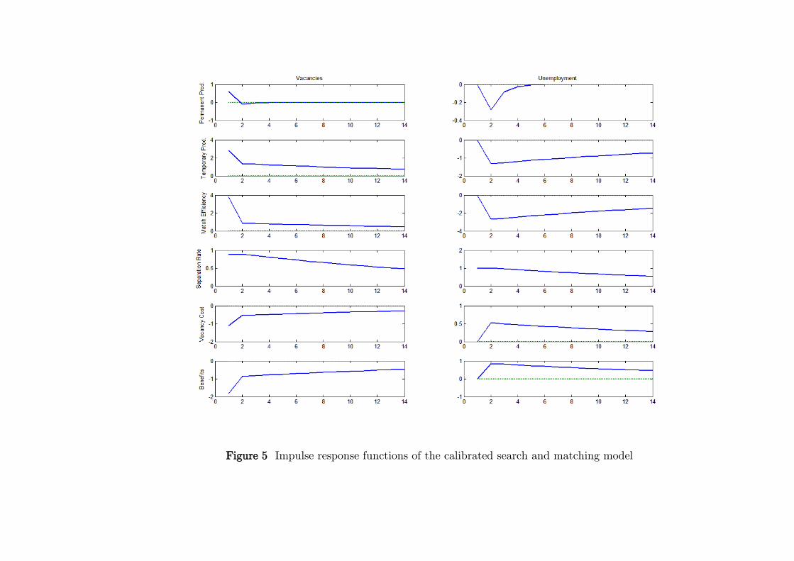
36

Figure 5 Impulse response functions of the calibrated search and matching model

37

Figure 6 Logarithm of real GDP and estimated permanent component, estimated transitory component of log real GDP, and Congressional Budget Office estimate of the output gap

38

Figure 7 Impulse response functions to a permanent output shock

39

Figure 8 Impulse response functions to the first transitory shock

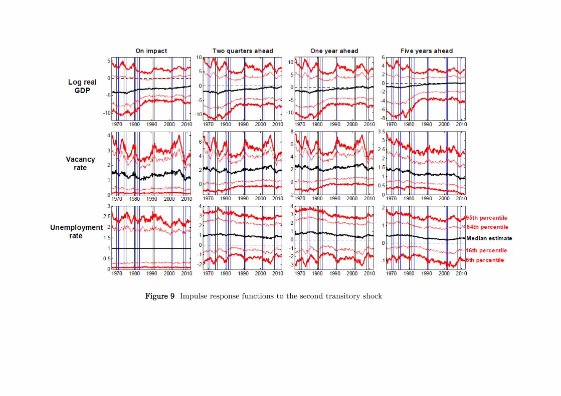
40

Figure 9 Impulse response functions to the second transitory shock

41

Figure 10 Fractions of innovation variance due to the permanent output shock

42

Figure 11 Fractions of innovation variance due to the two transitory shocks identified from sign restrictions

43

Figure 12 Evidence on the pro-cyclicality of the Beveridge curve

44

Figure 13 Business-cycle frequencies: average gain and coherence between vacancies and the unemployment rate conditional on the permanent and the transitory output shocks

45

Figure 14 Average gain of the unemployment rate onto vacancies at the business-cycle frequencies, as a function of individual parameters of the DSGE model (for parameter intervals around the modal estimates generated by the Random Walk Metropolis)