Department of Finance | Working Paper Series Page 1 of 2

Working Paper No. 01/21

Working Paper No. 01/21

Working Paper No. 01/21

— Department of Finance

Faculty of Business and Economics

Working Paper Series

Weather and Cross-Section of Stock Returns

Xi Li, Andrea Lu, Huijun Wang

Working Paper No. 06/21

May 2021

Weather and Cross-Section of Stock Returns

Xi Li

Andrea Lu

Huijun Wang1

This draft: May 2021

In this paper, we investigate a new channel for weather to predict the cross section of regional and individual stock returns via its impact on local payroll employment. We follow Wilson (2019) constructing a measure for local weather effect which is measured as the weather-based employment growth surprise. We find that the local weather effect can predict both one-month-ahead regional and individual stock returns. We find evidence of predictability arising via the employment channel and depend on weather information being geographically local. Further, the effect is stronger in stocks with more limits to arbitrage and in stocks located in regions with high temperature. Keywords: weather, stock returns JEL: G14, E32, O3, O4, L1, L2

1 Xi Li is from Walton College, University of Arkansas. Andrea is from Faculty of Business and Economics, University of Melbourne. Huijun Wang is from Faculty of Business and Economics, University of Melbourne and Auburn University. The authors thank seminar participants at Monash University for helpful comments.

Introduction

Economists show that weather and climate changes at annual or longer horizons could affect a variety of fundamental outcomes in the same periods. These outcomes include agriculture (e.g., Adams et al. 1990; Mendelsohn, Dinar, and Sanghi 2001; Schlenker and Roberts 2006; Deschenes and Greenstone 2007), productivity and economic growth (e.g., Dell, Jones, Olken 2012; Zivin and Neidell 2014; Colacito, Hoffmann, Phan 2019).

In finance, researchers hypothesize that simultaneous cloudy weather conditions negatively affect investor mood and as a result the same day stock returns. They find that stock indexes in the U.S. and internationally have a more positive daily return if the weather in the cities of the main stock exchanges is more sunny on the same day [e.g., Saunders 1993; Hirshleifer and Shumway 2003]. For individual stocks, although cloudy weather near firm headquarters is not related to the same day stock returns [e.g., Loughran and Schultz 2004], Goetzmann, Kim, Kumar, and Wang (2015) find that the weighted sky cloud cover across the regions of institutional investors holding the stock is negatively related to the sign of the same day returns for the stocks with the highest 20% of arbitrage costs.

A recent paper by Wilson (2019) focus on using weather to predict future returns on T-bonds and stock indexes. Different from both the literature using weather as a fundamental explanation for long term economic outcomes and the literature using weather as a mood explanation for the same day stock returns, he does not directly use weather as the predictive variable. Instead, he obtains the county level nowcast difference between t h e predicted employment growth given actual weather and the predicted employment growth given average weather for each county based on recursive out-of-sample regressions. Aggregating this county level nowcast difference of employment due to weather to the national level, he finds that the aggregated difference can predict not only employment surprises but also returns of U.S. T-bonds on the day that the actual employment number is reported. A trading strategy in U.S. T-bonds generate abnormal returns that are both statistically and economically significant. In his online appendix, he also shows that the aggregated difference can also weakly predict the returns of stock indexes on the employment report day.

Extending Wilson (2019), we examine whether the county level nowcast difference of employment due to weather in the headquarter regions of listed firms can predict the future stock returns for these firms at the monthly frequency. Also, different from the prior literature, we examine whether this difference can predict future stock returns at the monthly horizon. We find that the county level nowcast difference of employment due to weather is negatively related to at least the one-month-ahead returns significantly. The return spreads based on this difference generate a statistically significant abnormal returns but the magnitude of abnormal returns likely cannot overcome the associated arbitrage costs. The return spreads are greater and more statistically significant among the small, illiquid, and more volatile stocks, supporting a mispricing explanation.

Our results hold whether we examine the sample at the individual stock level or aggregate our sample stocks into regional portfolios. Our results are robust whether we define the region as a county or metropolitan statistical area (MSA). Our results are robust to a variety of common control variables. In fact, the county level nowcast difference of

employment due to weather has an extremely low correlation with most common variables that are shown to predict future stock returns, suggesting that it is a new anomaly. As in prior research, our results are not affected or driven by disastrous weather.

To avoid data snooping bias, we intentionally follow Wilson (2019) closely to measure the nowcast difference of employment due to weather. We do examine what radius from a region’s center that we use to measure weather would produce a nowcast difference that affect the stock returns the most. Too large or too small a radius may produce a weaker relation between the nowcast difference and stock returns. It seems that a radius of 50 miles originally used in Wilson (2019) produces the strongest relation.

In addition to the above mentioned literature of using weather or climate change to explain fundamental outcomes in the contemporaneous periods, our paper is also related to other papers using weather or climate changes to explain mortality (e.g., Deschenes and Moretti 2009; Barreca et al. 2016), crime and social unrest (e.g., Field 1992; Jacob, Lefgren, and Moretti 2007; Miguel, Satyanath, and Sergenti 2004), and politic changes (e.g., Bruckner and Ciccone 2011). Complementing this literature, we study how the county level nowcast difference of employment due to weather affects future returns of individual stocks.

In addition to the above mentioned literature of using cloudy weather to explain simultaneous stock returns on the same day, our paper is related to the extensive literature on the relation between weather and trading in individual stocks. Although researchers find mixed evidence that cloudy weather in the headquarter regions affect individual stock trading volume is mixed (e.g., Loughran and Schultz 2004, Goetzmann and Zhu 2005), Goetzmann et al. (2015) show that the weighted sky cloud cover across the regions of institutional investors in the stock can explain the perceived overpricing and trading in the stock. Cloudy weather also delays market reactions to earnings announcements (de Haan, Madsen, and Piotroski 2017) and the hiring and investment decisions of firms (Chhaochharia et al. 2019).

Instead of studying weather’s impact directly, we complement this literature by studying the impact of employment surprises due to weather on individual stock returns. Instead of the mood perspective, we study from the fundamental perspective. We also focus on whether employment surprises due to weather can predict future stock returns in the months ahead instead of the relation between weather and stock returns on the same day. We examine all the weather instead of focusing on the extent of cloudiness. We find that the county level nowcast difference of employment due to weather can predict at least one-month-ahead returns for the universe of stocks even though the results are also stronger in the subsample of stocks with high arbitrage costs. Thus, complementing this mood explanation that is based on mispricing, we provide evidence for a new mispricing channel that weather could affect stock returns.

An emerging literature shows that climate changes affect asset prices. For example, climate changes risks reduce housing prices (e.g., Baldauf, Garlappi, and Yannelis 2020; Bernstein, Gustafson, and Lewis 2019) and increase muni-bond yields (e.g., Painter 2020). Climate change risks also affect long run discount rates (e.g., Giglio, Maggiori, Rao, Stroebel, Weber 2021). To the extent that climate changes raise the frequency and severity of both

recurring and severe weather events and subsequently employment surprises related to weather, the impact of weather on future stocks that we observe may become stronger in the future.

The rest of the paper is organized as follows. In Section 2, we describe the data used in the paper and the construction of the local weather effect variable which captures the impact of weather on local payroll employment growth. Section 3 and Section 4 present evidence on local weather effect’s predictability of local stock returns and the performance of the local weather effect based trading strategies. In Section 5, we analyze the extent of how predictability varies across regions with different climate conditions. Section 6 concludes.

2. Data and county level nowcast employment difference

The weather data by county and month are from Global Historical Climatology Network Daily (GHCN-Daily) dataset. Employment data are available from the Quarterly Census of Employment and Wages (QCEW) which provides non-seasonally adjusted private nonfarm employment at county-level in monthly frequency. We use a sample of the firms listed on the New York Stock Exchange (NYSE), the American Stock Exchange (Amex) and Nasdaq. Stock prices and returns are from the Center for Research in Security Prices (CRSP). Accounting data are from COMPUSTAT. Institutional ownership data come from records of 13F form filings with the SEC, which are available through Thomson Reuters. The following subsections explain our data selection procedure, how we construct the county level nowcast difference of employment due to weather and the regional stock portfolios. It also report summary statistics of the local weather effect variable.

2.1 County level nowcast employment difference due to weather

We closely follow the methodology in Wilson (2019) to construct the county-level nowcast difference of employment due to weather. In this subsection, we outline the key steps in the construction of this nowcast difference.

We start by constructing the daily county-level weather variables using weather-station-level data from the GHCN-Daily dataset. We use five daily weather-station-level weather variables: the daily maximum temperature, an extreme hot day indicator that equals one if the maximum temperature on that day was above 90℉ (32.2℃), an extreme cold day indicator that equals one if the minimum temperature was below 30℉ (-1.1℃), precipitation in mm, and snowfalls in cm. We measure values of each weather variable at the county-level with inverse distance weighted averages of individual weather variable from the stations located within a 50 miles radius from the center of a county.2 The distance is the distance

2 Wilson (2019) took an additional step in the aggregation process by first aggregating station-level data to points on a 5-mile by 5-mile grid before mapping to coordinates of counties. The differences in our approaches are mostly due to convenience and our results are similar if we use the exact approach of Wilson (2019).

between a weather station and a county center. The geographic coordinates of weather stations and county centers are obtained from GHCN-Daily and the US Census. We then construct five monthly county-level weather variables using these daily county-level weather variables: the average daily maximum temperature, fraction of days in the month in which the maximum temperature was above 90℉, fraction of days in which the minimum temperature was below 30℉, average daily precipitation, and average daily snowfall.

To estimate the county level nowcast difference of employment due to weather, we use the following county-level panel model of the following form.

using an nowcasting method which fits estimates from a county-level panel model that estimates weather variables’ effects on monthly local private nonfarm employment growth to the real-time weather data in that month.

𝛥𝑐,𝑡 = 𝛾𝑡 + 𝛼𝑐,𝑚(𝑡),𝑑(𝑡) +∑∑𝛽𝑖𝜏𝑚𝑎𝑥𝑡𝑒𝑚𝑝

3

𝜏=0

4

𝑖=1

⋅ 1[𝑡 ∈ 𝑆𝑖] ⋅ 𝑤𝑐,𝑡−𝜏𝑚𝑎𝑥𝑡𝑒𝑚𝑝 +∑∑𝛽𝜏

𝑘

3

𝜏=0

4

𝑘=1

⋅ 𝑤𝑐,𝑡−𝜏𝑘 + 𝜖𝑐,𝑡,

where 𝛥𝑐,𝑡 is the change in log non-seasonally adjusted private nonfarm employment in county 𝑐 and month 𝑡. 𝛾𝑡 is a time fixed effect to absorb all national common shocks. 𝛼𝑐,𝑚(𝑡),𝑑(𝑡) is a county-specific calendar-month × decade fixed effect, which allows the

seasonal adjustment of employment growth by county and decade given that QCEW data are not available on the seasonally adjusted basis at the county level.

𝑤𝑐,𝑡−𝜏𝑚𝑎𝑥𝑡𝑒𝑚𝑝 is the average daily maximum temperature measure for county 𝑐 in month 𝑡 − 𝜏.

We interact it with a season indicator variable 1[𝑡 ∈ 𝑆𝑖] which is equal to 1 if month 𝑡 is in Season 𝑆𝑖 to allow the effects of maximum temperature on employment growth to differ by season. We define the following four seasons: Winter = December-February; Spring = March-May; Summer = June-August; and Fall = September-November. 𝑤𝑐,𝑡−𝜏

𝑘 is one of the other four

weather variables for county 𝑐 in month 𝑡 − 𝜏 and we constrain them to have the same effects

on employment growth across seasons. 𝛽𝑖𝜏𝑡𝑒𝑚𝑝 and 𝛽𝜏

𝑘 are the key parameters to be estimated

using data from the estimation window. They capture the effect of each of the five weather variables (k) by season (i) on the employment growth 𝜏 months ahead. 𝜏 takes value from 0 to 3 to allow weather to have not only a contemporaneous effect on the current month’s employment growth but also on future employment growth up to 3 months ahead. Wilson (2019) reports that lags beyond three months do not have any effect as shown by a Wald test that compares the three lag model to models with longer lags. These lags allow for both persistent and transitory (mean-reverting) weather effects.

In addition to the model described above, Wilson (2019) also considers a more flexible version of the model which further allows the effects of weather on employment growth to vary across the nine Census Bureau regions.3 He finds that allowing for regional-

3 Wilson (2017), which focuses exclusively on predicting employment growth instead of stock and bond returns, also experiments with models that allows every coefficient

heterogeneity in the above county panel model does not improve the explanatory power of weather for employment growth or bond returns. Further, allowing for regional heterogeneity would come at the cost of drastically increasing the number of coefficients by almost 9 times and potentially leads to overfitting and measurement errors. As a result, we do not assume regional heterogeneity in the effects of weather on employment growth.

We estimate the model using weighted least squares where the weights are log county employment in order to mitigate the influence of sparsely populated counties. These counties usually have fewer nearby weather stations, likely resulting in greater measurement error in their weather data. In addition, we winsorize employment growth at the first and 99th percentiles to mitigate the influence of measurement error and outliers in the dependent variable of this model.

To product the nowcast, we estimate the coefficients in the county-level panel model using recursive-expanding-estimation-window samples and apply these estimates on real-time weather variables to form the out-of-sample fitted values of the local employment growth in each county.

To account for the potential delay in county-level QCEW data release, we allow for a gap between the end of the estimation window and the nowcast formation time. Specifically, the nowcast of county 𝑐’s local employment growth in month 𝑡 is derived using values of county 𝑐’s weather variables in month 𝑡 and the slope coefficients estimated from the county-level panel model over a sample period that begins from January 1980 and ends eight-month prior to month 𝑡. To ensure a sufficient number of observations in the time-series, nowcasts are formed starting from January 2004: the out-of-sample fitted value of local employment growth in January 2004 is computed using weather variables in that month and the slope coefficients estimated over a sample from January 1980 to May 2003; the last out-of-sample fitted value in our sample, December 2018, is computed using weather variables in that month and the slope coefficients estimated over January 1980 to April 2018.

The coefficients and standard errors from estimating the county panel regression over the longest estimation sample in our sample period, January 1980 to April 2018, are shown in Table 1 for illustrative purposes. The first, second, third and fourth columns show the estimated coefficients and their standard errors on the contemporaneous values and the one-, two-, and three-month lagged values of the weather variables, respectively. We standardize all weather regressors by their full-sample standard deviation so that each coefficient represents the effect on local employment growth of a one standard deviation change in weather measure. We find document similar dynamic patterns of weather effects as in Wilson (2019). Specifically, higher temperatures have a positive and statistically significant contemporaneous effect on employment growth in all four seasons but with the

estimates in equation 1 to vary by nine Census Bureau regions and ten industries. In his model to create the county level nowcast difference of employment due to weather to predict returns, he prioritizes parsimony and focus on models with many fewer heterogeneity and thus coefficient estimates. The greater heterogeneity is not necessarily always better and could lead to overfitting and measurement error.

effect being relatively weaker in magnitude in fall; precipitation and snowfalls have negative and significant contemporaneous effects on employment growth; the higher the fraction of days in a month with extreme temperature, both hot and cold, the lower the employment growth; and, the lagged effects of weather generally are of opposite sign to the contemporaneous effect and tend to vanish after the first two lags.

In the final step, the local weather effect in a county is computed as the difference between the fitted employment growth given a county’s actual weather and the fitted employment growth given its historical average weather over calendar-month-decade. This approach allows us to better capture the shock element of the information about local employment growth that is caused by recent surprise in local weather condition but unlikely to be known or acted upon on by investors due to the infrequent release of local macroeconomic data. We can further construct the weather effect variable at the metropolitan statistical areas (MSAs) level by taking a weighted average of the county-level weather-based employment growth effects across its member counties using local employment as weights. Overall, we have a panel of county-level/MSA-level weather effect nowcasts from January 2004 to December 2018 covering 3006 counties in 384 MSAs.

2.2 Stocks, regional portfolios and firm/portfolios characteristics

Our initial sample of stocks includes all individual firms listed on the New York Stock Exchange (NYSE), the American Stock Exchange (Amex) and Nasdaq from CRSP. Following convention (see, e.g. Coval and Moskowitz 1999, 2001; Koughran and Schultz, 2005; Pirinsky and Wang, 2006; Hong et al., 2008; Korniotis and Kumar, 2013), we use corporate headquarter location to proxy firm location and individual stocks are matched with weather effect of counties in which firms’ corporate headquarters are located. We obtain firms’ historical headquarter addresses using the Compustat Snapshot database and company 10-Ks filed with the SEC through EDGAR with webcrawling algorithms. We require stocks to have an identifiable county location and a minimum price of $5 to be included in the sample. Upon matching stock returns to the county-level weather effects, we arrive at a sample with 7065 unique firms located in 790 unique counties.

We form county-level and MSA-level regional portfolios and compute their returns by taking the market-capitalization-weighted average over returns of firms with corporate headquarters located in that county/MSA. To minimize potential measurement error, we require each regional portfolio to have a minimum of 5 stocks. As a result, we yield a sample of 124 county-level portfolios and 81 MSA-level portfolios in an average month.4

4 We tried some alternative values for the minimum number of stocks (1 to 10) required in construction the regional stock portfolios. The average number of portfolios decreases as the minimum requirement increases. Specifically, the average number of county-level regional portfolios with a valid weather effect variable in a given month reduces from 566 to 89 when the minimum stock number requirement increases from 1 to 10. Nevertheless, the choice of minimum requirement does not qualitatively drive our results.

A list of firm characteristics are used as control variables in the empirical analyses presented in later sections. These include size (log of market capitalization from the previous month), book-to-market ratio (BE/ME), market beta, institutional ownership ratio, idiosyncratic volatility, stock liquidity, past one-month return, cumulative return on the stock from 𝑡 − 12 to 𝑡 − 2, and cumulative return on the stock from 𝑡 − 36 to 𝑡 − 13. The corresponding characteristics for regional portfolios are computed as the market capitalization weighted average of stock characteristics across stocks of firms with corporate headquarters located in that region.

2.3 Descriptive statistics

Table 2 presents summary statistics for the county-level and MSA-level weather-fitted employment growth surprise (the weather effects) in monthly frequency. The univariate statistics in Panel A compare the mean, standard deviation and autocorrelation coefficient of the weather effects against those of the employment growth predicted by historical average weather (average weather effect) and the actual employment growth. Univariate statistics show that the surprise component of the weather effect is slight more volatile than the actual employment growth but much less volatile than the average weather effect both at the county- and MSA-level. Weather effect is also less autocorrelated comparing to the actual employment growth and the average weather predicted employment growth; the latter has a high autocorrelation coefficient of greater than 0.60. Panel B reports the weather effect’s correlations with the average weather effect, the actual employment growth, as well as with some common stock characteristics variables. We find that the estimated weather effect has a positive but low correlation with the average weather effect and a minimal correlation with the actual employment growth. Meanwhile, the weather effect, both at the county- and MSA-level, has almost no correlation with the list of common stock characteristics including size (log of market capitalization from the previous month), book-to-market ratio (BE/ME), market beta, institutional ownership ratio (IO ratio), idiosyncratic volatility, stock liquidity, past one-month return, cumulative return on the stock from 𝑡 − 12 to 𝑡 − 2, and cumulative return on the stock from 𝑡 − 36 to 𝑡 − 13. The low correlations are expected as our measure of weather effect capture local weather effect on local payroll employment growth rather than being stock specific. Further, these evidence also indicate that the weather effect carries information about local employment growth that are relevant to local stocks beyond what common stock characteristics can capture. These information are yet to be revealed in the macroeconomic data release and thus unlikely to be captured by accounting variables.

3 Return predictability of weather effects

3.1 Baseline predictability regression

In this section, we examine the relation between local weather effect and future stock returns. We investigate to what extent the payroll employment growth nowcasts fitted using weather data can explain the cross-sectional variation in performance of individual stocks and regional portfolios while controlling for some common firm characteristics. We consider three sets of test assets in our analyses: individual stocks (Model 1), the county-level regional

portfolios (Model 2), and the MSA-level regional portfolios (Model 3). We match future returns to their closest local measure of weather effect: we use the county-level weather effect to study the relation between local weather effect and future returns of individual stocks and county-level portfolios; we use the MSA-level weather effect to analyze the performance of MSA-level regional portfolios. We adopt the Fama and MacBeth (1973) regressions to study the estimated local weather effect’s predictability on stock returns. Specifically, each month, we estimate a cross-sectional regression of test assets’ one-month-ahead returns on the estimated local weather effect variable and four stock characteristics that are known to explain stock returns: size, market beta, BE/ME and IO ratio. We report the time-series average of coefficients from the cross-sectional regressions along with their time-series 𝑡-statistics computed using Newey-West standard errors. Table 3 presents the results. Model 1 shows that returns of individual stocks in the next month are positively and significantly related to the estimated local weather effect of the county in which the companies’ corporate headquarters are located indicating that the weather-fitted employment growth surprise can predict performance of local stocks in the near future. In other words, weather’s impact on the latest month’s local payroll employment growth contains valuable yet new information that are relevant to firms located in the nearby geographical area. These relevant information, due to the infrequent release of local macroeconomic data and investors’ lack of ability to interpret or understand weather’s impact on local employment, are yet to be fully absorbed in the stock prices in the current period.

We also find evidence of the local weather effect’s predictability on future returns of the geography-based regional portfolios. Using regional portfolios as test assets allows us to better understand the aggregate impact of the weather-fitted local employment growth nowcasts on the performance of stocks in the local geographical region. Model 2 and Model 3 present results using the county-level regional stock portfolios and MSA-level regional stock portfolios as test assets. The average cross-sectional coefficients on the weather effect variables are positive and statistically significant at 1% level in both cases.

Taken together, results presented in Table 3 provide some strong evidence in favor of the estimated local weather effect having a positive effect on stock performance of local firms in the following month, both at the individual stocks level and at the regional stock portfolio level. The effect is robust to controlling for common firm characteristics in cross-sectional regressions. The source of the predictability is likely due to local weather condition’s importance influence on local employment condition which in turn have a strong impact on local business’ performance in the near future.

3.2 Source of the new information embedded in the local weather effect

The construction of the local weather effect is crucial in extracting the information in real-time weather data that precisely captures the component that is new to the public but relevant about the current local labour market condition. To demonstrate this point, we put several alternative measures to test and compare their return predictability with that of the local weather effect variable. We consider three sets of alternative variables: the five county-level weather variables that were used in estimating the local weather effect variable, the county-level employment growth, and the nowcasts of local employment growth formed

using historical average weather data (as opposed to being the surprise component as in our local weather effect variable). In all three sets of tests, we use variables’ value in month 𝑡 − 1 to predict returns of local stocks/portfolios in month 𝑡 and the predictability analyses are done using the Fama MaeBeth (1973) regressions. We conduct the tests on two sets of test assets: individual stocks and the county-level regional portfolios.5 Table 4 present the results. We find that the local employment growth and weather variables on their own have no predictive power on local stocks/regional-portfolios’ next month return as none of the coefficients have any statistical significance. Our local weather effect remains to have a significant return predictability power after controlling for the county-level weather variables and the employment growth: the economic magnitude of the effect is at a similar level of 0.0477 and the effect is statistically significant at the 5% level. This result suggests that understanding the relationship between the local labour market condition and weather is important for extracting out the relevant information about the current local labour market in real-time weather data. The information extracted following our methodology is what is important in determining local business’ short term performance. In addition, we find that the average-fitted local weather effect has a much weaker impact on local stocks/portfolios’ future returns: the effect on county-level regional portfolios are statistically insignificant; and, the effect on individual stocks is significant only at the 10% level with a much smaller coefficient of 0.0062. These results further highlight the importance of using real-time weather data. It is indeed the surprise component in the weather condition that matters more to local business than information that people have already known.

3.3 Geographical relevance of the local weather effect

In our paper, the county-level local weather effect is measured as the nowcasts of local payroll employment growth fitted using real-time county-level weather variables and estimates from a county-level panel regression that models the relation between employment growth and the current and past values of local weather variables. The county-level weather variables used in forming the nowcasts are constructed using weather-station-level data from stations located within a 50 miles radius from the county center. The choice of the maximum distance used in assigning weather stations to a county imposes a tradeoff: choosing a short distance could potentially leads to an insufficient representation of local weather condition and some counties with no nearby weather station within the chosen range; meanwhile, choosing a long distance may lead to inclusion weather data from geographically distant weather stations of which’s weather data are less relevant to local employment of that county.

Table 5 displays the Fama and MacBeth (1973) regressions results using the local weather effect variables constructed using four different input values for the maximum radius distance between weather stations the county center: 20 miles, 50 miles, 70 miles and 100

5 We exclude the MSA-level regional portfolios as the test asset in analyzing the return predictability of these alternative variables because the weather variables are constructed at the county-level.

miles. Although we mitigate the effect of distance selection by using an inverse-distance-weighted procedure when we aggregate weather-station-level weather data to county-level, results indicate the choice of distance still matters. Results show that, in terms of magnitude, the local weather effect’s predictability on local stock returns decreases nearly monotonically as the maximum distance between weather stations and county center increases. However, while a closer distance yields a higher predictive coefficient, it also brings more noise to the measure as reflected in the lower 𝑡-statistics for the weather variable. The local weather effect’s predictability on local stocks’ next-month return has the strongest statistical significance when the maximum distance between a weather station and the county center is set at 50 miles: the 𝑡-statistic for the coefficient of the weather variable peaks when the distance is set to be less or equal to 50 miles. Similar patterns can be found in the adjusted 𝑅2s.

These findings supports our choice of using 50 miles as the maximum radius distance between weather stations and county center in the construction of the county-level weather variables as it provides a good balance between capturing the local weather condition both quantitatively and qualitatively. These findings also demonstrate that the effect of local weather is localized - weather affects future performance of local businesses via the employment channel in a geographically sensitive manner.

4. Weather-based trading strategies

4.1 Performance of weather-based trading strategies

To further assess the predictability of the local weather effect on stock returns and to evaluate its economic significance, we adopt an approach commonly used in the literature to investigate the relation between returns and relevant stock characteristics: the portfolio sorting approach. We start by forming five portfolios on the basis of the local weather effect variable over the pool of individual stocks. We use the county-level weather effect variable measured in month 𝑡 − 1 to form portfolios of stocks in month 𝑡. A firm gets added to the low weather effect portfolio if its local county weather effect variable is below the 20th percentile in the cross-section of local weather effects in the previous month. Correspondingly, a firm gets added to the high weather effect portfolio if its weather effect variable exceeds the 80th percentile. Three more portfolios are formed using the 40th and 60th percentiles as break-points. We also form a zero-cost investment strategy that longs the high weather effect portfolio and shorts the low weather effect portfolio. The sample period starts in February 2004 and ends in January 2019.

Panel A of Table 6 shows the time-series averages of the equally weighted monthly returns on the portfolios of stocks sorted by the estimated local weather effect and the average returns of the high-minus-low zero-cost portfolio. Firms with low weather effects experienced an average return of 0.72% per month during the sample period; on the other hand, the portfolio of firms with weather effects in the highest quintile earn an average monthly return of 0.93%. The 21 basis point difference in average monthly returns between firms with high and low weather effects is economically sizable and statistically significant at 5% level.

We also perform portfolio sorting analysis on the county-level and MSA-level regional portfolios and results are shown in Panel B and C of Table 6. Given that the number of regional portfolios, which can be used to form the weather-effect-sorted portfolios, is much fewer comparing to that of individual stocks, we reduce the number of portfolios sorted on the weather effect to 3 to ensure a sufficient number of assets within each weather-effect-sorted bin. A county-level or MSA-level portfolio gets added to the high weather effect portfolio if the corresponding county’s/MSA’s weather effect variable recorded in the previous month is in the top one third of the cross-section of local weather effects; a county-level or MSA-level regional portfolio gets added to the low weather effect portfolio if the corresponding local weather effect variable is in the bottom one third; and, the rest fall into another portfolio. We find that the average return of county-level regional portfolios in the high local weather effect portfolio is 23 basis points per month higher than the average return of county-level portfolios located in the low local weather effect portfolio and the return difference is significant at 5%. Similarly, the average return difference between MSA-level portfolios located in the highest- and lowest local weather effect group is at a similar level of 20 basis points per month while being statistically significant. In both cases, the average returns monotonically increase with the estimated local weather effects recorded in the previous period.

Overall, the results in table 6 suggest that stocks located in areas with high weather-fitted nowcasts of payroll employment growth consistently outperform stocks located in areas with low weather-fitted nowcasts of payroll employment growth in the next month and this finding holds both at the individual stocks level and at the regional portfolios level.

4.2 Persistence of return predictability

In the baseline portfolio sorting analysis, we find that the real-time-weather-fitted nowcasts of local employment growth can predict future returns of local firms. Stocks located in counties with high local weather effects in a give month tend to have higher returns in the following month. To further investigate the speed of which the weather-driven employment growth news is absorbed and traded upon by stock-market investors, we examine the persistence of the local weather effect’s predictability on local stocks’ future returns. We repeat the portfolio sorting analysis in the previous subsection allowing for a longer horizon between the month when the local weather effect is estimated and that of future stock returns. Same as previously, we construct the local-weather-effect-sorted spread portfolios over three sets of test assets: individual stocks, the county-level regional portfolios and the MSA-level regional portfolios. In constructing the high-minus-low portfolio, we sort stocks (regional portfolios) into five (three) groups based on their values of the local weather effect variable.

Table 7 reports the average future, up to 12 months ahead, returns of the high-minus-low zero-cost portfolio sorted on the value of stocks’ local weather effect. We find that the impact of local weather effect on local stocks is short lived with the high-minus-low local-weather-effect return spread formed over individual stocks only being statistically significant when looking at returns one-month ahead. Although the high-minus-low local-weather-effect return spread continue to take a positive value in future stock returns up to 4 months ahead, the local-weather-effect-based premia are statistically insignificant and are much smaller in

magnitude. Specifically, the return difference between stocks with the highest and lowest local weather effects 2, 3, and 4 months ahead are at 9, 9, and 18 basis points, respectively, comparing to the significant 21 bps spread in the next-month. We also observe a gradual reversal starting from the 5th month and lasting for another three months with the effect being statistically significant in month 6 (21 bps).

We find similar results in the county-level and MSA-level regional portfolios: the positive average future returns of the high-minus-low zero-cost portfolio sorted on the value of stocks’ local weather last for 4 months after portfolios’ formation but the return spreads are not statistically significant beyond two-month in small economic magnitude. However, in contrast to the case of individual stocks, we do not observe an evident reversal, both in forms of economic magnitude and statistical significance, when using regional portfolios as test assets.

We also report the local-weather-effect-sorted return spreads 6 to 12 months after formation month. In most of these horizons, the local-weather-effect-sorted spreads are small in magnitude and statistically insignificant. The only odd exception is in month +10: the average returns of the local-weather-effect-sorted high-minus-low portfolio in the 10th month following their formation are positive and significant with large economic magnitude: the spread is at 22, 29 and 26 bps when formed over individual stocks, county-level regional portfolios and MSA-level regional portfolios. We do not have a good explanation for the observed positive effect and nor for why they occur in this particular horizon by not in others. However, given that weather information updates daily and macroeconomic data are updated multiple times in 10-month time, we think it is unlikely that the positive spread is due to the local weather effect 10 months back.

Overall, we find that local weather effect’s predictability is short-lived and information carried by weather about local employment growth is quickly and efficiently priced in without experiencing major over- or under-reaction. These finding suggest that the local weather effect’s predictability arises from an information advantage from real-time data rather than a mispricing caused by investors’ persistent behavior bias.

4.3 Firm characteristics and performance of trading strategies

We examine the local weather effect variable’s relation to future returns within subsets of stocks or regional portfolios. To do so, we first sort stocks into tertile groups according to stock characteristic and then sort within each characteristic-tertile group by stocks’ corresponding values of the local weather effect variable into quintiles. Stocks are equal-weighted within these 15 portfolios. Table 8 displays the average monthly returns of the top and bottom local-weather-effect-sorted quintile portfolios formed using subset of stocks with common characteristics within each characteristic-sorted subset as well as the average returns for the corresponding zero-cost high-minus-low local-weather-effect-hedged portfolio for each subset of stocks. We consider a list of characteristics including size, stock liquidity, idiosyncratic volatility, visibility, and fraction of share held by transient institutional investors. To ensure a sufficient number of assets within each portfolio, we only perform double sorting on stocks but not on regional portfolios.

Among the list of characteristics we consider, the first three are well known measures of arbitrage costs: size, stock liquidity and idiosyncratic volatility. We find that the local-weather-effect-based high-minus-low return spread is the highest among small size stocks: the difference in returns between firms with highest and lowest local weather effects is a significant 30bps per month among the smallest firms; meanwhile, no detectable difference between the high- and low-weather-effect group exists in the largest firms. We also sort stocks into three liquidity categories using Amihud (2002)’s illiquidity measure. Following Amihud (2002), a stock’s illiquidity is measured as the average absolute daily return per dollar volume over the last 12 months, with a minimum observation requirement of 150. We place a stock into the low (high) liquidity category if its Amihud measure is in the bottom (top) one third in the cross-section of all stocks in our sample. We find that the local-weather-effect-sorted high-minus-low spread is the highest among firms with low liquidity, at 28bps per month, and the spread monotonically decreases as we move to stocks with better liquidity. A similar monotonic pattern is observed when sorting first on stock’s idiosyncratic volatility which is measured as the standard deviation of daily excess return residuals adjusted by the Fama-French three-factor model estimated using daily returns over the past 3 months following Ang et al. (2009). The local weather premium is stronger among the high idiosyncratic volatility stocks. Overall results from double-sorting suggest that return predicting power of the weather-fitted nowcasts of local employment growth seems to increase with measures of limits to arbitrage.

We also examine the local weather effect’s return predictability in stocks with different levels of visibility. Specifically, we define low (the bottom one third) and high (the top one third) firm visibility subsamples using the Hong et al. (2008) measure of stock visibility. We could not find a monotone relation between the weather-based return spread and stock visibility. The local-weather-effect-based return spread is the highest in the middle group: stocks with the highest local weather effect in this group earn a significant 22 bps higher return per month comparing to stocks with the lowest local weather effect. Meanwhile, the local-weather-effect-premium are statistically insignificant and economically smaller among the high- and low-visibility stocks at 16 bps and 17 bps per month respectively.

We show that high levels of transient institutional ownership, i.e. the fraction of shares held by institutions with short investment horizons, are associated with an over-weighting of near-term expected earnings and thus making these stocks being more prone to myopic mispricing. We find no clear relation between the local-weather-effect-based return spreads and stocks’ transient ownership. The difference in returns between firms with highest and lowest local weather effects is high in stocks with the highest or lowest transient ownership categories but low in the middle category.

5. Local climate condition and return predictability

So far, we have shown that the nowcasts of local payroll employment growth formed using real-time weather data are informative about performance of local stocks in the near future. Our sample covers a broad range of over 7000 firms located in 790 unique counties. There is a big dispersion in their geographic locations and their local climate conditions also vary. Using heat shocks (i.e. days with temperature above 90F) a proxy of weather shocks, Park

(2016) found that the sensitivities of local payroll to weather shocks vary with county’s climate condition. Specifically, they find that places more prone to extreme heat stress exhibit significantly lower temperature sensitivities than colder places and they argue that adaption is the reason behind this reduced sensitivity.

Inspired by Park (2016), we investigate whether the local weather effect’s predictive power on stock returns vary across stocks located in regions with different climate conditions. Following Park (2016), we sort our sample into two groups based on historical average temperature of counties where stocks’ corporate headquarters are located. The low temperature group contains stocks/regional-portfolios located in counties with average temperature below the median of counties in the US; the high temperature group contains stocks/regional portfolios located in counties with average temperature above median.

We estimate the cross-sectional regressions of one-month-ahead returns on the local weather effect variable within each temperature-based subsample while controlling for four stock characteristics (size, market beta, BE/ME, and IO ratio). Table 9 reports the time-series average of coefficients from cross-sectional regressions for the low- and high-temperature subsamples along with their time-series 𝑡-statistics. We find that the local weather effect has a stronger predictive power on next-month returns of stocks in countries with high average temperature. In Model (1) and (4), where we use individual stocks as test assets, the coefficient on the county-level weather predicted employment growth is 0.0324 among stocks located in low temperature counties and weak statistically; meanwhile the coefficient is more than double at a significant 0.0681 among stocks located in high temperature counties. Similar results can be found using regional portfolios as test assets. In fact, the predictability of the local weather effect is only statistically significant for firms located in high temperature regions. Our findings are seemingly contrasting to ones of in Park (2016) which sensitivities of local labour market to heat shocks is higher in cold places. The difference could be due to two reasons. First, Park(2016) analyze the sensitivity of labour market to weather whereas we use real-time weather data to extract information about local employment growth that are relevant to the performance of local stocks. Second, Park (2016) focus solely on one type of weather shock, the heat shocks, as opposed to a broad range of weather variables in this paper. Our results offer an alternative channel for weather to affect local economic condition and in turn affect performance of local firms: weather in general can have a strong effect on local economic condition but the infrequent update/release data on local macroeconomic condition fail to reveal the relevant information to investors and thus lead to a short term mispricing in the stock market. This mispricing seem to be stronger in high temperature regions.

6. Conclusion

In this paper, we investigate a new channel for weather to predict the cross section of regional and individual stock returns via its impact on local payroll employment. We follow Wilson (2019) constructing a measure for local weather effect which is measured as the weather-based employment growth surprise. We find that the local weather effect can predict both one-month-ahead regional and individual stock returns. We find evidence of predictability arising via the employment channel and depend on weather information being

geographically local. Further, the effect is stronger in stocks with more limits to arbitrage and in stocks located in regions with high temperature.

References

Adams, R., Rosenzweig, C., Peart, R., Ritchie, J., McCarl, B., Glyer, D., Curry, R., Jones, J., Boote, K., Allen Jr., L., 1990. Global Climate Change and US Agriculture. Nature 345 (6272): 219–224.

Yakov A., 2002. Illiquidity and stock returns: cross-section and time-series effects. Journal of Financial

Markets 5, 31–56.

Ang, A . , Hodrick, R . , Xing, Y . , Zhang., X., 2009. High idiosyncratic volatility and low returns: I nternational and further U.S. evidence. Journal of Financial Economics 91, 1–23.

Baldauf, M., Garlappi, L., Yannelis, C., 2020. Does climate change affect real estate prices? Only

if you believe in it, Review of Financial Studies 26, 1256-1295.

Barreca, A., Clay, K., Deschenes, O., Greenstone, M., Shapiro, J., 2016. Adapting to Climate

Change: The Remarkable Decline in the US Temperature-Mortality Relationship over the

Twentieth Century, Journal of Political Economy 124, 105-159.

Bernstein, A., Gustafson, M., Lewis, R., 2019. Disaster on the horizon: The price effect of sea

level rise, Journal of Financial Economics 134, 253-272.

Brückner, M., Ciccone., A., 2011. Rain and the Democratic Window of Opportunity.

Econometrica 79, 923–947.

Burke, M., Emerick., K., 2016. Adaptation to Climate Change: Evidence from U.S. Agriculture.

American Economic Journal: Economic Policy 8, 106–40.

Brian J Bushee. Do institutional investors prefer near-term earnings over long-run value? Contemporary Accounting Research, 18(2):207–246, 2001.

Brian J. Bushee & Henry L. Friedman, 2016. Disclosure standards and the sensitivity of returns to

mood, Review of Financial Studies 29, 787-822.

Chhaochharia, V., Kim, D., Korniotis, G., Kumar, A., 2019. Mood, Firm Behavior, and Aggregate

Economic Outcomes. Journal of Financial Economics 132, 427-450.

Colacito, R., Hoffmann, B., Phan, T., 2019. Temperature and growth: A panela analysis of the

United States, Journal of Money, Credit and Banking 51, 313-368.

Cortes, K., Duchin, R., Sosyura, D., 2016. Clouded judgment: The role of sentiment in credit

origination, Journal of Financial Economics 121, 392-413.

Joshua D Coval and Tobias J Moskowitz. Home bias at home: Local equity preference in domestic portfolios. The Journal of Finance, 54(6):2045–2073, 1999.

Joshua D Coval and Tobias J Moskowitz. The geography of investment: Informed trading and asset prices. Journal of political Economy, 109(4):811–841, 2001.

Dehaan, E., Madsen, J., Piotroski, J., 2017. Do Weather-Induced Moods Affect the Processing of

Earnings News? Journal of Accounting Research 55, 509-550.

Dell, M., Jones, B., Olken., B., 2012. Temperature Shocks and Economic Growth: Evidence from the

Last Half Century. American Economic Journal: Macroeconomics 4, 66–95.

Deschenes, O., Greenstone., M., 2007. The Economic Impacts of Climate Change: Evidence from Agricultural Output and Random Fluctuations in Weather. American Economic Review 97, 354–385.

Deschenes, O., Moretti., E., 2009. Extreme Weather Events, Mortality, and Migration. Review of Economics and Statistics 91, 659–681.

Field, S., 1992. The Effect of Temperature on Crime. British Journal of criminology 32, 340–351

Fama, E., MacBeth., J., 1973. Risk, return, and equilibrium: empirical tests. Journal of Political Economy 81, 607–636.

Giglio, S., Maggiori, M., Rao, K., Stroebel, J., Weber, A., 2021. Climate Change and Long-Run

Discount Rates: Evidence from Real Estate, Review of Financial Studies, Forthcoming.

Goetzmann, W., Kim, D., Kumar, A., Wang, Q. 2015. Weather-Induced Mood, Institutional

Investors, and Stock Returns. Review of Financial Studies 28, 73-111.

Goetzmann, W., Zhu, N. 2005. Rain or Shine: Where is the Weather Effect? European Financial

Management 11, 559-578.

Hirshleifer, D., Shumway, T., 2003. Good Day Sunshine: Stock Returns and the Weather. Journal

of Finance 58, 1009-1032.

Hong, H., Kubik, J., Stein., J., 2008, The only game in town: Stock-price consequences of local bias. Journal of Financial Economics 90, 20–37.

Jacob, B., Lefgren, L., Moretti., E., 2007. The Dynamics of Criminal Behavior: Evidence from

Weather Shocks, Journal of Human Resources 42, 489–527.

Korniotis, G., and Kumar, A., 2013. State-Level Business Cycles and Local Return Predictability,

Journal of Finance 68, 1037-1096.

Loughran, T., Schultz, P., 2004. Weather, Stock Returns, and the Impact of Localized Trading

Behavior. Journal of Financial and Quantitative Analysis, 39, 343-364.

Loughran, T., Schultz, P., 2005. Liquidity: Urban versus rural firms, Journal of Financial Economics 78, 341–374.

Mendelsohn, R., Dinar, A., Sanghi., A., 2001. The Effect of Development on the Climate

Sensitivity of Agriculture. Environment and Development Economics 6, 85–101.

Miguel, E., Satyanath, S., Sergenti., E., 2004. Economic Shocks and Civil Conflict: An

Instrumental Variables Approach. Journal of political Economy 112, 725–53.

Painter, M., 2020. An Inconvenient Cost: The Effects of Climate Change on Municipal Bonds,

Journal of Financial Economics 135, 468-482.

Jisung Park. Will we adapt? temperature shocks, labor productivity, and adaptation to climate change in the united states. Working Paper, 2016.

Pirinsky, C., Wang., Q., 2006. Does corporate headquarters location matter for stock returns? Journal of Finance 61, 1991–2015.

Saunders, E., 1993. Stock Prices and Wall Street Weather. American Economic Review 83, 1337-

1345.

Schlenker, W., Roberts., M., 2006. “Nonlinear Effects of Weather on Corn Yields. Review of

Agricultural Economics 28, 391–98.

Wilson., D., 2017. The impact of weather on local employment: Using big data on small places. Working paper.

Wilson, D., 2019. Clearing the fog: The predictive power of weather for employment reports and their

asset price responses. American Economic Review: Insights 1, 373–388.

Zivin, J., Neidell, M., 2014. Temperature and the Allocation of Time: Implications for Climate

Change. Journal of Labor Economics 32, 1-26.

Table 1: Weather’s economic effects on local payroll employment growth

This table presents coefficients and standard errors of key parameters from estimating the county-level panel regression that estimates weather’s economic effects on local employment. The right-hand-side variable is the monthly change in log non-seasonally-adjusted nonfarm employment at the county-level. The right hand variables include the contemporaneous value of five county-level weather variables and their past 3 lagged values. The five county-level weather variables include the average daily high temperature, precipitation (mm), snowfall (cm), the fraction of days in a month with the maximum temperature being above 90F, and the fraction of days with the minimum temperature being below 30F. We allow the average maximum daily temperature to have differential effect on log employment growth across four seasons (Spring, Summer Fall and Winter). A time fixed effect and a county-specific calendar-month-decade fixed effect are also included. Standard errors presented in parentheses are robust to heteroskedasticity. The estimation period is from January 1980 to April 2018.

(1) (2) (3) (4)

Contemporaneous 1st lag 2nd lag 3rd lag

Avg. daily high temp - Spring 0.056*** -0.042*** -0.049*** 0.000

(0.00) (0.01) (0.01) (0.01)

Avg. daily high temp - Summer 0.051*** -0.017*** -0.011** -0.014***

(0.01) (0.00) (0.00) (0.00)

Avg. daily high temp - Fall 0.018*** -0.003 0.002 0.012

(0.01) (0.01) (0.01) (0.01)

Avg. daily high temp - Winter 0.091*** -0.040*** -0.032*** 0.004

(0.01) (0.01) (0.01) (0.01)

Precipitation (mm) -0.037*** 0.017*** 0.022*** 0.008**

(0.00) (0.00) (0.00) (0.00)

Snowfall (cm) -0.010*** 0.004 0.003 0.004

(0.00) (0.00) (0.00) (0.00)

% days low temp < 30F -0.080*** -0.004 0.036*** 0.028**

(0.01) (0.01) (0.01) (0.01)

% days high temp > 90F -0.018** -0.021*** -0.021*** -0.008

(0.01) (0.01) (0.01) (0.01)

Adj. 𝑅2 0.548

N 1,254,201

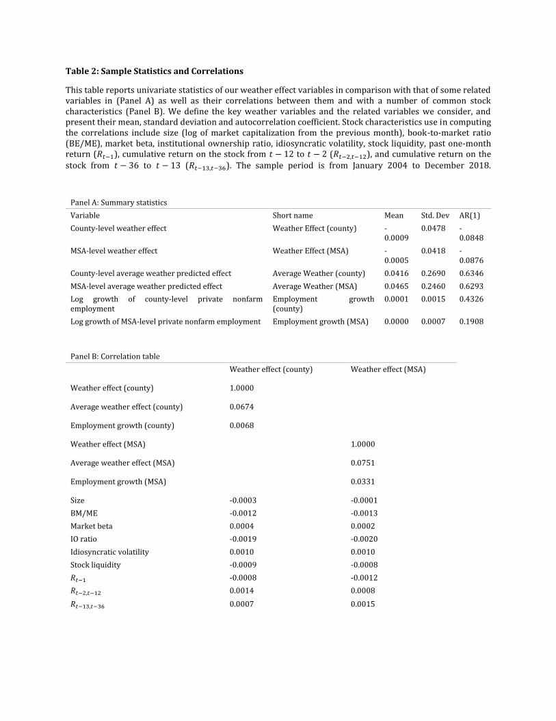
Table 2: Sample Statistics and Correlations

This table reports univariate statistics of our weather effect variables in comparison with that of some related variables in (Panel A) as well as their correlations between them and with a number of common stock characteristics (Panel B). We define the key weather variables and the related variables we consider, and present their mean, standard deviation and autocorrelation coefficient. Stock characteristics use in computing the correlations include size (log of market capitalization from the previous month), book-to-market ratio (BE/ME), market beta, institutional ownership ratio, idiosyncratic volatility, stock liquidity, past one-month return (𝑅𝑡−1), cumulative return on the stock from 𝑡 − 12 to 𝑡 − 2 (𝑅𝑡−2,𝑡−12), and cumulative return on the

stock from 𝑡 − 36 to 𝑡 − 13 (𝑅𝑡−13,𝑡−36). The sample period is from January 2004 to December 2018.

Panel A: Summary statistics

Variable Short name Mean Std. Dev AR(1)

County-level weather effect Weather Effect (county) -0.0009

0.0478 -0.0848

MSA-level weather effect Weather Effect (MSA) -0.0005

0.0418 -0.0876

County-level average weather predicted effect Average Weather (county) 0.0416 0.2690 0.6346

MSA-level average weather predicted effect Average Weather (MSA) 0.0465 0.2460 0.6293

Log growth of county-level private nonfarm employment

Employment growth (county)

0.0001 0.0015 0.4326

Log growth of MSA-level private nonfarm employment Employment growth (MSA) 0.0000 0.0007 0.1908

Panel B: Correlation table

Weather effect (county) Weather effect (MSA)

Weather effect (county) 1.0000

Average weather effect (county) 0.0674

Employment growth (county) 0.0068

Weather effect (MSA) 1.0000

Average weather effect (MSA) 0.0751

Employment growth (MSA) 0.0331

Size -0.0003 -0.0001

BM/ME -0.0012 -0.0013

Market beta 0.0004 0.0002

IO ratio -0.0019 -0.0020

Idiosyncratic volatility 0.0010 0.0010

Stock liquidity -0.0009 -0.0008

𝑅𝑡−1 -0.0008 -0.0012

𝑅𝑡−2,𝑡−12 0.0014 0.0008

𝑅𝑡−13,𝑡−36 0.0007 0.0015

Table 3: Impact of the local weather effect on the cross section of expected returns

This table presents results for the Fama-MacBeth regressions that study the impact of the local weather effect on the cross-section of expected stock returns. The local weather effect measures the nowcasts of local payroll employment growth fitted using real-time weather data and estimates from a county-level panel regression. Cross-sectional regressions of stock returns on the local weather effect and a host of firm characteristics are run every month on the universe of individual stocks/regional portfolios over the period February 2004 to January 2019. The cross sections of returns in month 𝑡 are regressed on a constant, log of size (market capitalization in month 𝑡 − 1), BE/ME, market beta, institutional ownership ratio, and the local weather effect variable. These regressions are repeated for regional stock portfolios formed at the county level and the MSA level, respectively. The local weather effect variable we use is measured at the county-level in regressions with individual stocks and county-level portfolios as test assets and at the MSA level in regressions with MSA-level portfolios. The time-series average of the coefficient estimates and their associated time-series 𝑡-statistics computed using Newey-West standard errors (in parentheses) are reported.

(1) (2) (3)

Stocks County portfolios MSA portfolios

Weather (County) 0.0465*** 0.0651***

(2.80) (2.98)

Weather (MSA) 0.0796 ***

(2.77)

Log(size) 0.0002 -0.0001 -0.0002

(0.34) (-0.21) (-0.43)

BE/ME 0.0005 -0.0015 -0.0013

(0.89) (-0.81) (-0.51)

Market beta -0.0018 -0.0064 -0.0042

(-0.62) (-1.40) (-0.84)

IO ratio 0.0041** 0.0052 0.0023

(2.09) (1.43) (0.56)

Intercept 0.0046 0.013 0.0142

(0.70) (1.51) (1.57)

Adj. 𝑅2 0.0336 0.1075 0.1316

Average observations 2,736 120 79

Table 4: Impact of other related variables on the cross section of expected returns

This table presents results that compare the impact of the county-level local weather effect variable on the cross-section of expected stock returns with that of some related county-level variables. The local weather effect measures the nowcasts of county-level payroll employment growth fitted using real-time weather data and estimates from a county-level panel regression. We consider three sets of related variables: the average weather effect which measures the nowcasts of county-level payroll employment growth fitted using historical average weather data, the actual employment growth, and five county-level weather variables. The actual employment growth is measured as the monthly change in log non-seasonally-adjusted county-level nonfarm employment. The five county-level weather variables include the average daily high temperature, precipitation (mm), snowfall (cm), the fraction of days in a month with the maximum temperature being above 90F, and the fraction of days with the minimum temperature being below 30F. Cross-sectional regressions of stock returns on each of the three sets of variables and a host of firm characteristics are run every month on the universe of individual stocks/regional portfolios over the period February 2004 to January 2019. The cross sections of returns in month 𝑡 are regressed on a constant, log of size (market capitalization in month 𝑡 − 1), BE/ME, market beta, institutional ownership ratio, and the chosen set of variable(s). These regressions are repeated for stock portfolios formed at the county level. The time-series average of the coefficient estimates and their associated time-series 𝑡-statistics computed using Newey-West standard errors (in parentheses) are reported.

Stocks County portfolios

(1) (2) (3) (4) (5) (6) (7) (8)

Weather (FIPS) 0.0477** 0.0647**

(2.21) (2.38)

Average weather (FIPS)

0.0062** 0.0038

(1.94) (0.96)

Employment growth

-0.0001

-0.0001 -0.0004

-0.0009

(-0.29) (-0.35) (-0.55) (-1.10)

Avg. daily high temp

0 0 -0.0001 -0.0001

(-0.08) (-0.44) (-1.00) (-1.20)

Precipitation -0.0001

0 -0.0002 -0.0001

(-0.5) (0.24) (-1.00) (-0.32)

Snowfall 0.6811 0.7316 -0.2745 -0.2477

(0.58) (0.63) (-0.14) (-0.13)

% days high temp > 90F

0.0042 0.0005 0.0364 0.0368

(0.10) (0.01) (1.32) (1.33)

% days low temp < 30F

0.0317 0.0228 0.0617 0.055

(0.91) (0.65) (1.11) (1.06)

Intercept 0.0045 0.0049 0.0066 0.0079 0.0116 0.0116 0.0231* 0.0267**

(0.68) (0.75) (0.81) (0.97) (1.35) (1.33) (1.94) (2.14)

Controls Y Y Y Y Y Y Y Y

Adj. 𝑅2 0.0334 0.0327 0.0353 0.036 0.1078 0.1052 0.1226 0.129

Avg obs per month

2,736 2,736 2,736 2,736 120 120 120 120

Table 5: Impact of the local weather effect on the cross section of expected returns: by radius distance between weather station and county center

This table presents results for the Fama-MacBeth regressions that study the impact of the local weather effect on the cross-section of expected stock returns. We present results using local weather effects constructed with different radius distance. The local weather effect measures the nowcasts of local payroll employment growth fitted using real-time weather data and estimates from a county-level panel regression. Weather(dist ≤ 20 (50/70/100) miles) is the local weather effect estimated using county-level variables constructed based on weather data from stations located within a 20 (50/70/100) miles radius from the center of a county. Cross-sectional regressions of stock returns on the local weather effect and a host of firm characteristics are run every month on the universe of individual stocks/regional portfolios over the period February 2004 to January 2019. The cross sections of returns in month 𝑡 are regressed on a constant, log of size (market capitalization in month 𝑡 − 1), BE/ME, market beta, institutional ownership ratio, and the local weather effect variable. These regressions are repeated for regional stock portfolios formed at the county level and the MSA level, respectively. The local weather effect variable we use is measured at the county-level in regressions with individual stocks and county-level portfolios as test assets and at the MSA level in regressions with MSA-level portfolios. The time-series average of the coefficient estimates and their associated time-series 𝑡-statistics computed using Newey-West standard errors (in parentheses) are reported.

Stocks County portfolios MSA portfolios

(1) (2) (3) (4) (5) (6) (7) (8) (9) (10) (11) (12)

Weather (≤ 20 miles)

0.067** 0.0934** 0.1045* .

(2.09) (1.99) (1.82)

Weather (≤ 50 miles)

0.0465*** 0.0651*** 0.0796***

(2.80) (2.98) (2.77)

Weather (≤ 70 miles)

0.0376** 0.0505*** 0.0698**

(2.42) (2.57) (2.35)

Weather (≤ 100 miles)

0.0305** 0.0397** 0.0582**

(2.40) (2.51) (2.49)

Controls yes yes yes yes yes yes yes yes yes yes yes yes

Adj 𝑅2 0.0331 0.0336 0.0334 0.0334 0.1123 0.1135 0.1062 0.1063 0.1322 0.1326 0.1321 0.1323

N 2682 2736 2736 2736 118 120 120 120 78 79 79 79

Table 6: Returns to the local-weather-effect-sorted portfolios

This table presents the time-series average of monthly returns on the equal-weighted portfolios sorted according to the levels of the local weather effect. The local weather effect measures the nowcasts of county-level payroll employment growth fitted using real-time weather data and estimates from a county-level panel regression. Test assets used in forming these portfolios include individual stocks (Panel A), county-level regional portfolios (Panel B), and MSA-level regional portfolios (Panel C). Each month, stocks (regional-portfolios) are sorted into quintiles (tertiles) on the basis of the corresponding local weather effect level and one-month-ahead equal-weighted returns are computed on the quintile (tertile) portfolios. High-Low is a zero-cost portfolio that is long in the quintile (tertile) portfolio with the largest local weather effect (high) and short in portfolio with the smallest local weather effect (low). The time-series average of month returns on the portfolios and their associated Newey West 𝑡-statistics are presented. The sample period is February 2004 to January 2019.

Panel A: Returns on portfolios formed over individual stocks according to the levels of

the county-level local weather effect

Weather

Low Q2 Q3 Q4 High High-Low

Stocks 0.0072* 0.0077** 0.0076** 0.0084** 0.0093** 0.0021**

(1.87) (1.99) (2.06) (2.25) (2.37) (2.21)

Panel B: Returns on portfolios formed over county-level regional portfolios

according to the levels of the county-level local weather effect

Weather

Low T2 High High-Low

County portfolios 0.0071** 0.0082** 0.0094*** 0.0023**

(2.00) (2.48) (2.82) (2.33)

Panel C: Returns on portfolios formed over MSA-level regional portfolios

according to the levels of the MSA-level local weather effect

Weather

Low T2 High High-Low

MSA portfolios 0.0074** 0.0079** 0.0094*** 0.0020*

(2.11) (2.39) (2.80) (1.72)

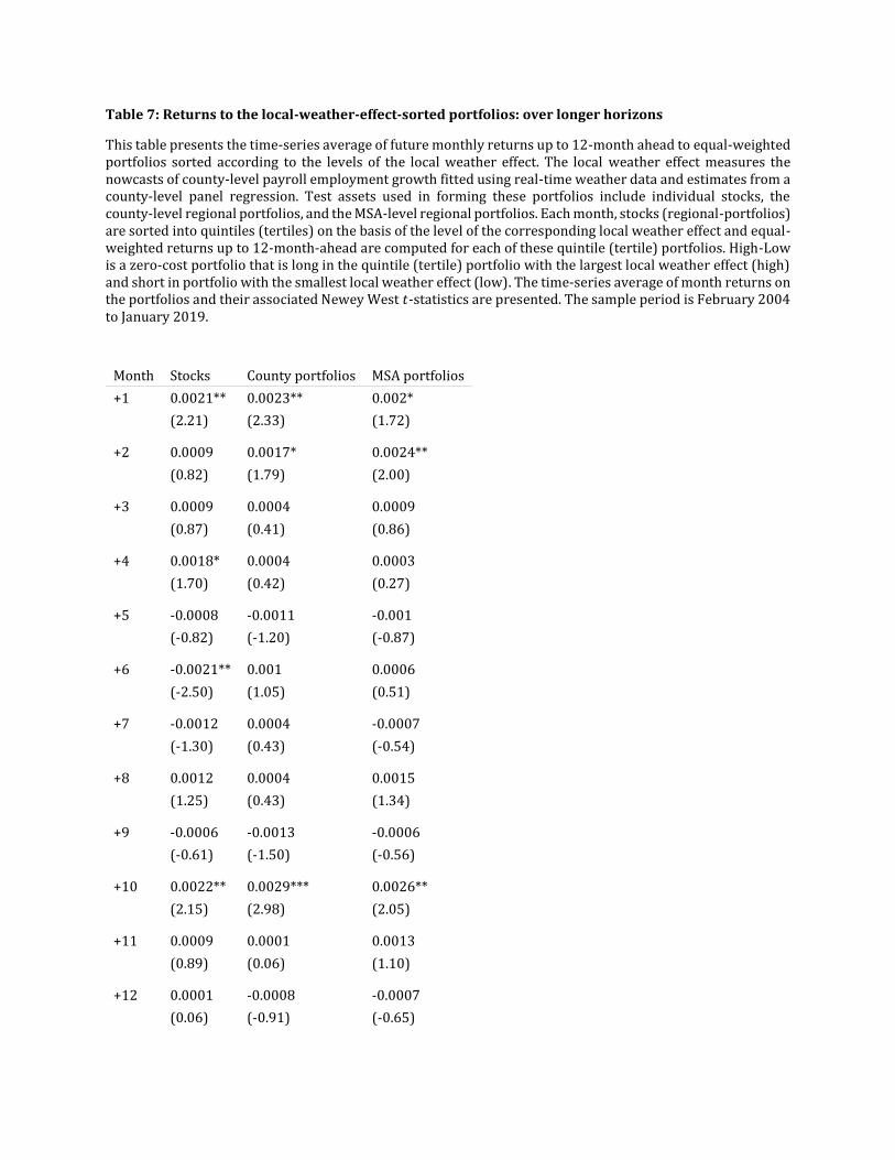
Table 7: Returns to the local-weather-effect-sorted portfolios: over longer horizons

This table presents the time-series average of future monthly returns up to 12-month ahead to equal-weighted portfolios sorted according to the levels of the local weather effect. The local weather effect measures the nowcasts of county-level payroll employment growth fitted using real-time weather data and estimates from a county-level panel regression. Test assets used in forming these portfolios include individual stocks, the county-level regional portfolios, and the MSA-level regional portfolios. Each month, stocks (regional-portfolios) are sorted into quintiles (tertiles) on the basis of the level of the corresponding local weather effect and equal-weighted returns up to 12-month-ahead are computed for each of these quintile (tertile) portfolios. High-Low is a zero-cost portfolio that is long in the quintile (tertile) portfolio with the largest local weather effect (high) and short in portfolio with the smallest local weather effect (low). The time-series average of month returns on the portfolios and their associated Newey West 𝑡-statistics are presented. The sample period is February 2004 to January 2019.

Month Stocks County portfolios MSA portfolios

+1 0.0021** 0.0023** 0.002*

(2.21) (2.33) (1.72)

+2 0.0009 0.0017* 0.0024**

(0.82) (1.79) (2.00)

+3 0.0009 0.0004 0.0009

(0.87) (0.41) (0.86)

+4 0.0018* 0.0004 0.0003

(1.70) (0.42) (0.27)

+5 -0.0008 -0.0011 -0.001

(-0.82) (-1.20) (-0.87)

+6 -0.0021** 0.001 0.0006

(-2.50) (1.05) (0.51)

+7 -0.0012 0.0004 -0.0007

(-1.30) (0.43) (-0.54)

+8 0.0012 0.0004 0.0015

(1.25) (0.43) (1.34)

+9 -0.0006 -0.0013 -0.0006

(-0.61) (-1.50) (-0.56)

+10 0.0022** 0.0029*** 0.0026**

(2.15) (2.98) (2.05)

+11 0.0009 0.0001 0.0013

(0.89) (0.06) (1.10)

+12 0.0001 -0.0008 -0.0007

(0.06) (-0.91) (-0.65)

Table 8: Returns to the local-weather-effect-sorted portfolios controlling for stock characteristics

This table presents the time-series average of monthly returns of equal-weighted portfolios formed on the basis of the local weather effect over subsets of stocks with common stock characteristics. The local weather effect measures the nowcasts of county-level payroll employment growth fitted using real-time weather data and estimates from a county-level panel regression. Each month, stocks are first sorted into tertiles on a given stock characteristics then sorted into quintiles portfolios on the basis of the corresponding local weather-predicted employment growth. Stock characteristics we consider include size, stock liquidity, idiosyncratic volatility, visibility and fraction of outstanding shares held by transient institutional investors. Within each characteristic tertile, we also form a zero-cost hedge portfolio which is long in the quintile portfolio consisting stocks with the largest local weather effect (high) and short in portfolio consisting stocks with the smallest local weather effect. We report the one-month-ahead equal-weighted returns of the top weather quintile, the bottom weather quintile (Low) and the zero-cost hedge portfolio (High-Low) formed using stocks in each characteristic tertile. The time-series average of monthly returns on the portfolios and their associated Newey West 𝑡-statistics are presented. The sample period is February 2004 to January 2019.

Weather Weather

Low High High-Low

Low High High-Low

Size (Market capitalization)

Visibility

Small 0.0060 0.0090** 0.0030** Low 0.0081* 0.0097** 0.0016

(1.59) (2.28) (2.51) (1.87) (2.17) (1.15)

Medium 0.0079* 0.0093** 0.0014 Middle 0.008** 0.0102** 0.0022**

(1.87) (2.14) (1.11) (2.02) (2.54) (1.97)

Large 0.0077** 0.0095*** 0.0017 High 0.0084** 0.0101*** 0.0017

(2.10) (2.60) (1.51) (2.30) (2.71) (1.40)

Transient investors ownership

Low 0.0059* 0.0087** 0.0028** Low 0.0053 0.0078** 0.0024**

(1.65) (2.29) (2.35) (1.54) (2.27) (2.02)

Middle 0.0079* 0.0098** 0.0018 Middle 0.0081** 0.0097** 0.0016

(1.85) (2.25) (1.56) (2.09) (2.42) (1.47)

High 0.0079** 0.0092** 0.0013 High 0.0081* 0.0107** 0.0027**

(2.08) (2.44) (1.08) (1.86) (2.47) (1.98)

Small 0.0093*** 0.0093 *** 0.0000

(3.17) (3.08) (-0.05)

Medium 0.0081** 0.0103*** 0.0022**

(2.11) (2.60) (2.01)

High 0.0046 0.0081 0.0035**

(0.98) (1.63) (2.06)

Table 9: The effect of local temperature

This table presents results for the Fama-MacBeth regressions that study the impact of the local weather effect on the cross-section of expected stock returns in subsamples of regions with different historical temperature. The local weather effect measures the nowcasts of county-level payroll employment growth fitted using real-time weather data and estimates from a county-level panel regression. Stocks/portfolios are first sorted into two groups based on the average historical temperature of the region in which stocks/portfolios are located. Cross-sectional regressions of stock returns on the local weather effect and a host of firm characteristics are run every month on the universe of regional portfolios/individual stocks over the period February 2004 to January 2019 for each subsample. The cross sections of stock returns at time 𝑡 are regressed on a constant, size, BE/ME, market beta, institutional ownership ratio, and the weather-predicted local employment growth variable. These regressions are repeated in stock portfolios formed at the county-level and MSA-level, respectively. The local weather effect is measured at the county level for regressions with individual stocks and the county-level regional portfolios as test assets, and measured at the MSA-level for regressions with the MSA-level regional portfolios. Panel A presents results from the low historical temperature subsample and Panel B presents results from the high historical temperature subsample. The time-series average of the coefficient estimates and their associated time-series 𝑡-statistics (in parentheses) are reported in the style of Fama and MacBeth (1973).

Low temperature High temperature

(1) (2) (3) (4) (5) (6)

County MSA County MSA

Stocks portfolios portfolios Stocks portfolios portfolios

Weather (County) 0.0324* 0.0315 0.0681*** 0.0691**

(1.82) (1.45) (2.62) (2.01)

Weather (MSA) 0.0509 0.0788*

(1.56) (1.84)

Log(size) 0.000 0.0001 0.0002 0.0003 -0.0007 -0.0011

(0.07) (0.24) (0.32) (0.56) (-1.20) (-1.70)

BE/ME 0.0009 -0.0007 -0.0015 -0.0002 -0.0031 -0.0023

(1.13) (-0.40) (-0.57) (-0.27) (-0.92) (-0.53)

Market beta -0.0012 -0.0039 -0.0019 -0.0024 -0.0067 -0.0059

(-0.41) (-0.75) (-0.34) (-0.80) (-1.30) (-1.00)

IO ratio 0.0042* 0.0041 0.0002 0.0038 0.0024 0.0021

(1.87) (0.96) (0.04) (1.90)** (0.44) (0.36)

Intercept 0.005 0.0063 0.0063 0.0043 0.0259** 0.0318**

(0.74) (0.60) (0.60) (0.65) (2.11) (2.14)

Adj 𝑅2 0.0373 0.1093 0.1396 0.033 0.1225 0.1596

Average obs. 1303 63 40 1433 57 39

Appendix

Table A. 1 Returns to the local-weather-effect-sorted portfolios: by radius distance between weather station and county center

This table presents the time-series average of monthly returns on the equal-weighted portfolios sorted according to the levels of the local weather effect estimated using different radius distance. The local weather effect measures the nowcasts of county-level payroll employment growth fitted using real-time weather data and estimates from a county-level panel regression. Test assets used in forming these portfolios include individual stocks (Panel A), county-level regional portfolios (Panel B), and MSA-level regional portfolios (Panel C). Each month, stocks (regional-portfolios) are sorted into quintiles (tertiles) on the basis of the corresponding local weather effect level and one-month-ahead equal-weighted returns are computed on the quintile (tertile) portfolios. High-Low is a zero-cost portfolio that is long in the quintile (tertile) portfolio with the largest local weather effect (high) and short in portfolio with the smallest local weather effect (low). In each panel we present results using local weather effect constructed using different radius distance. The local weather effect with distance ≤ 20 (50/70/100) miles is estimated using county-level variables constructed using weather data from stations located within a 20 (50/70/100) miles radius from the center of a county. The time-series average of month returns on the portfolios and their associated Newey West 𝑡-statistics are presented. The sample period is February 2004 to January 2019.

Panel A: individual stocks

Weather

Test assets Distance Low Q2 Q3 Q4 High High-Low

Stocks ≤ 20 miles 0.0076** 0.0077** 0.0081** 0.0084** 0.0088** 0.0012

(1.97) (2.03) (2.11) (2.23) (2.27) (1.38)

≤ 50 miles 0.0072* 0.0077** 0.0076** 0.0084** 0.0093** 0.0021**

(1.87) (1.99) (2.06) (2.25) (2.37) (2.21)

≤ 70 miles 0.0075** 0.0078** 0.0078** 0.0084** 0.0088** 0.0013

(1.96) (2.01) (2.12) (2.23) (2.25) (1.35)

≤ 100 miles 0.0073* 0.0080** 0.0077** 0.0083** 0.009** 0.0016*

(1.92) (2.07) (2.08) (2.23) (2.28) (1.67)

Panel B: County portfolios

Weather

Test assets Distance Low T2 High High-Low

County portfolios ≤ 20 miles 0.0073** 0.0081** 0.0093*** 0.002**

(2.08) (2.48) (2.78) (2.08)

≤ 50 miles 0.0071** 0.0082** 0.0094*** 0.0023**

(2.00) (2.48) (2.82)*** (2.33)

≤ 70 miles 0.0073** 0.0078** 0.0095*** 0.0021**

(2.10) (2.34) (2.86) (2.24)

≤ 100 miles 0.0077** 0.0074** 0.0096*** 0.0018*

(2.21) (2.20) (2.89) (1.91)

Panel C: MSA portfolios

Weather

Test assets Distance Low T2 High High-Low

MSA portfolios ≤ 20 miles 0.0078** 0.0075** 0.009*** 0.0012

(2.22) (2.31) (2.68) (0.99)

≤ 50 miles 0.0074** 0.0079** 0.0094*** 0.0020*

(2.11) (2.39) (2.80) (1.72)

≤ 70 miles 0.0076** 0.0081** 0.0089*** 0.0013

(2.17) (2.45) (2.66) (1.19)

≤ 100 miles 0.0075** 0.0080** 0.0092*** 0.0016

(2.13) (2.44) (2.70) (1.42)

Department of Finance | Working Paper Series Page 2 of 2

fbe.unimelb.edu.au/finance