Work ing PaPer Ser ieSno 1557 / j une 2013

on the international SPilloverS of uS Quantitative eaSing

Marcel Fratzscher, Marco Lo Duca and Roland Straub

In 2013 all ECB publications

feature a motif taken from

the €5 banknote.

note: This Working Paper should not be reported as representing the views of the European Central Bank (ECB). The views expressed are those of the authors and do not necessarily reflect those of the ECB.

© European Central Bank, 2013

Address Kaiserstrasse 29, 60311 Frankfurt am Main, GermanyPostal address Postfach 16 03 19, 60066 Frankfurt am Main, GermanyTelephone +49 69 1344 0Internet http://www.ecb.europa.euFax +49 69 1344 6000

All rights reserved.

ISSN 1725-2806 (online)EU Catalogue No QB-AR-13-054-EN-N (online)

Any reproduction, publication and reprint in the form of a different publication, whether printed or produced electronically, in whole or in part, is permitted only with the explicit written authorisation of the ECB or the authors.This paper can be downloaded without charge from http://www.ecb.europa.eu or from the Social Science Research Network electronic library at http://ssrn.com/abstract_id=2269642.Information on all of the papers published in the ECB Working Paper Series can be found on the ECB’s website, http://www.ecb.europa.eu/pub/scientific/wps/date/html/index.en.html

AcknowledgementsThe paper was previously circulated under the title “A global monetary tsunami? On the spillovers of US Quantitative Easing”. We would like to thank participants at the 2012 AEA, EEA and EFA meetings, the 2012 NBER IFM programme meeting, the German Economic Association Monetary Theory meeting, the Banco de España-World Bank conference on “Debt and Credit, Growth and Crises”, at seminars at the Federal Reserve Board, the IMF, the ECB, ZEW and Cass Business School, and in particular our discussants Eduardo Fernández Arias, Joe Gagnon, Kate Phylaktis Ole Rummel and Carmen Reinhart. The views presented in the paper are those of the authors and do not necessarily represent the views of the European Central Bank or the Eurosystem.

Marcel FratzscherDIW Berlin and CEPR; e-mail: mfratzscher@diw.de

Marco Lo DucaEuropean Central Bank; e-mail: marco.lo_duca@ecb.europa.eu

Roland StraubEuropean Central Bank; e-mail: roland.straub@ecb.europa.eu

Abstract

The paper analyses the global spillovers of the Federal Reserve’s unconventional monetary policy measures. First, we find that Fed measures in the early phase of the crisis (QE1) were highly effective in lowering sovereign yields and raising equity markets, especially in the US relative to other countries. Fed measures since 2010 (QE2) boosted equities worldwide, while they had muted impact on yields across countries. Yet Fed policies functioned in a pro-cyclical manner for capital flows to emerging markets (EMEs) and a counter-cyclical way for the US, triggering a portfolio rebalancing across countries out of EMEs into US equity and bond funds under QE1, and in the opposite direction under QE2. Second, the impact of Fed operations, such as Treasury and MBS purchases, on portfolio allocations and asset prices dwarfed those of Fed announcements, underlining the importance of the market repair and liquidity functions of Fed policies. Third, we find no evidence that FX or capital account policies helped countries shield themselves from these US policy spillovers, but rather that responses to Fed policies are related to country risk. The results thus illustrate how US unconventional measures have contributed to portfolio reallocation as well as a re-pricing of risk in global financial markets. JEL Codes: E52, E58, F32, F34, G11. Keywords: monetary policy, quantitative easing, portfolio choice, capital flows, Federal Reserve, United States, policy responses, emerging markets, panel data.

2

Non-technical summary

The 2007-09 global financial crisis triggered unprecedented policy interventions in the United

States. Besides the more standard counter-cyclical policy measures, the Federal Reserve

launched a new set of non-standard policy tools, which have been labeled as credit-easing or

quantitative easing policies (QE). In the period after the collapse of Lehman Brothers in

September 2008 (often referred to as QE1), measures included (i) an extension of liquidity

operations to support banks and markets, and (ii) large-scale asset purchases (LSAP) of GSE

debt, agency debt, mortgage-backed securities (MBS) and Treasury securities. By contrast,

the second main push by the Federal Reserve started in the second half of 2010 (QE2) and

concentrated primarily on purchases of US Treasury securities.

While most of the debate has focused on the effects of QE on the US economy, foreign

policy-makers – in particular in emerging markets– argued that QE policies have created

excessive global liquidity and caused an acceleration of capital flows to EMEs. In turn, this

capital flow surge is widely blamed for appreciation pressures on EME currencies and a

build-up of financial imbalances in EMEs.

To shed some light on this issue, the paper analyses the effects of the Federal Reserve’s

unconventional policies on the US and on 65 foreign financial markets. Importantly, the paper

extends the existing literature by investigating the effects on both global asset prices and

capital flows. For this purpose, we use a relatively novel database of daily portfolio flows into

bond and equity mutual funds, taking primarily a US investor perspective. In this way, we can

track capital injections into funds (portfolio flows) across countries.

We analyze different types of US unconventional monetary policy measures (liquidity

operations, purchases of MBS and of US Treasuries) in order to understand whether and why

QE1 and QE2 have exerted different effects on US and foreign markets. In contrast with most

of the literature on US QE, which has focused narrowly on announcement effects, we make a

distinction between announcements of Fed interventions and the actual market operations.

The results in the paper illustrate how US monetary policy since 2007 has contributed to

portfolio reallocation as well as a re-pricing of risk in global financial markets. First, we find

that Fed measures in the early phase of the crisis (QE1) were highly effective in boosting

bond and equity prices, especially in the US, and led to US dollar appreciation. Conversely,

QE2 boosted equity prices worldwide and led to US dollar depreciation. Yet Fed policies

functioned in a pro-cyclical manner for capital flows to EMEs and in a counter-cyclical way

for the US. QE1 triggered a portfolio rebalancing across countries out of emerging markets

(EMEs) into the US, while QE2 triggered rebalancing in the opposite direction. This finding

may be interpreted as lending support to the concerns expressed by policymakers in EMEs.

3

Second, the impact of Fed operations, such as Treasury and MBS purchases, on portfolio

allocations and asset prices dwarfed that of Fed announcements. This result underlines the

importance of the market repair and liquidity functions of Fed policies. Third, there is no

evidence that FX or capital account policies helped countries shield themselves from

spillovers. We find instead that heterogeneity in the response to Fed policies is related to

country risk.

The results suggest that there are indeed global spillovers and externalities from monetary

policy decisions in advanced economies. However, the paper is mute on whether such

externalities are overall positive or negative for other economies. The potentially undesirable

effects of these measures on the pro-cyclicality of EME capital flows need to be weighed

against potential benefits such as higher economic activity and a better financial market

functioning in the global economy.

4

"This crisis started in the developed world. It will not be overcome … through … quantitative

easing policies that have triggered … a monetary tsunami, have led to a currency war and

have introduced new and perverse forms of protectionism in the world."

President Rousseff of Brazil (2012)

1 Introduction The 2007-09 global financial crisis triggered unprecedented policy interventions by central

banks around the globe. After cutting policy rates to close to the zero lower bound, several

central banks started conducting non-standard measures. The Federal Reserve has been one of

the most active, implementing several types of non-standard measures during different

periods. In the period after the collapse of Lehman Brothers in September 2008 (often

referred to as QE1), measures aimed at repairing the functioning of financial markets and

focused mainly on liquidity operations to support banks and on large-scale asset purchases

(LSAP) of GSE debt, agency debt, mortgage-backed securities (MBS) and Treasury

securities. By contrast, the second main push by the Federal Reserve started in the second half

of 2010 (QE2) and concentrated primarily on purchases of US Treasury securities, with the

primary aim of stimulating the US economy by lowering yields, and pushing up asset prices

in riskier market segments inducing thereby positive wealth effects. In September 2011, the

Federal Reserve launched “Operation Twist”, a commitment to extend the maturity of

securities held on its balance sheet, followed by the announcement in September 2012 of a

third round of QE, focusing on the purchase of MBS.

While most of the debate has focused on the effects of QE on the US economy, foreign

policy-makers – in particular in emerging markets, as highlighted by the above quote by

President Rousseff of Brazil – have been criticizing the Fed’s policies, arguing that these have

created excessive global liquidity, and thus caused the massive acceleration of capital flows to

EMEs since 2009. In turn, this capital flow surge is widely blamed for appreciation pressures

on EME currencies, a build-up of financial imbalances and asset price bubbles in EMEs, high

credit growth and the threat of an over-heating of the domestic economies. As the above

quote suggests, some see the unconventional monetary policy measures of advanced

economies even as a form of protectionism.

There is indeed a hole in the literature about global effects of unconventional monetary

policies, with most of the literature focusing on the effects of QE on US domestic markets1

1 Most of this work focuses on QE1, generally finding empirical evidence that the announcements of the Fed’s purchases lowered US yields (e.g. Gagnon et al. 2011; D’Amico and King 2011; Wright, 2011), with similar evidence for the UK (Joyce et al. 2011), while yielding more mixed evidence for the effectiveness of the Term Auction Facility (Thornton, 2010) and MBS purchases (Hancock and Passmore 2011, Stroebel and Taylor 2012). Hamilton and Wu (2011) discuss the effectiveness of

5

and their underlying channels. Through the portfolio balance channel, QE may not only

trigger a portfolio rebalancing towards more risky domestic assets, but also towards foreign

assets. Similarly, a signaling about future US economic conditions and policy rates, or

changes in risk and liquidity premia in the US, and confidence effects are likely to have

implications for economic conditions and financial markets elsewhere in the world. However,

with a few notable exceptions, little analysis has been conducted so far to gauge these

spillover effects.2

This paper analyses the effects of the Federal Reserve’s QE both on the US and on 65 foreign

financial markets. Importantly, the paper does not only investigate the effects on asset prices,

as most of the literature does, but also on portfolio decisions by investors. This is important as

portfolio decisions are central for identifying the portfolio balance channel of Fed policies.

For this purpose, we use a relatively novel database of high-frequency, daily portfolio flows

into bond and equity mutual funds, taking primarily a US investor perspective. The advantage

of the data is that we do not only track capital injections into US bond and equity funds, but

also inflows into EME and other advanced economy funds.

We analyze different types of US unconventional monetary policy measures (liquidity

operations, purchases of MBS and of US Treasuries) in order to understand whether and why

QE1 and QE2 have exerted different effects on US and foreign markets. An important

distinction we make is between announcements of Fed interventions and the actual market

operations. Most of the literature on US QE has focused narrowly on the effects

announcements of the two large-scale asset purchase (LSAP) programs, but not the actual

operations and purchases, assuming that only the announcement contain new information,

while the latter do not, or do much less so.

Turning to the empirical results, a first key result highlights the fundamental difference

between QE1 and QE2. QE1 measures have been highly effective in lowering long term

yields in the US and elsewhere and in supporting equity prices (especially in the US).

However, they also triggered a strong global rebalancing of investor portfolios out of EMEs

and into US equity and bond funds, thus also inducing overall appreciation of the US dollar.

By contrast, QE2 measures appear to have been largely ineffective in lowering yields

worldwide, have caused sizeable capital outflows, mainly into EME equities, and a marked

US dollar depreciation.

This evidence thus suggests the presence of a portfolio balance channel. QE1 measures

induced mainly a portfolio rebalancing across countries, while QE2 functioned both through a

unconventional monetary policy tools at the zero lower bound. Krishnamurthy and Vissing-Jorgensen discuss the transmission channels of quantitative easing. 2 Neely (2010) and Bauer and Neely (2012) finds significant and sizeable effects of the Fed’s LSAP on sovereign yields in a small sample of other advanced economies. Chen et al. (2011) document significant spillovers of QE into Asian financial markets.

6

portfolio rebalancing across asset classes (from bonds into equities) and across countries. In

particular the US Treasury purchases under QE2 triggered a large portfolio rebalancing out of

bond markets globally, primarily into EME equity markets.

A second major finding of the paper is that the Fed’s LSAP announcements had overall

comparatively smaller effects than actual Fed operations. This is particularly the case for

portfolio decisions and asset prices outside the US (in EMEs and other advanced economies

AE). This is an important finding because it suggests that investors in no way fully priced in

and reacted only to Fed announcements. To the contrary, the impact of Fed operations has

been dominant, an analysis of which has been missing so far in the literature. We argue that

this finding is sensible, as mere Fed announcements that e.g. aim at repairing dysfunctional

markets alone are insufficient to trigger such a repair. Moreover, actual operations may

contain new information and may help coordinate market participants, a fact that has become

apparent also in non-standard measures of other central banks, such as the ECB’s 3-year long-

term refinancing operations (LTROs) of December 2011 and February 2012.

Third, in terms of economic significance, the effects of US QE measures on capital flows to

EMEs have been relatively small compared to other factors, but they have exacerbated the

pro-cyclicality of EME capital flows. In cumulative terms, US unconventional monetary

policy measures together explain EME net equity inflows of 5% and EME net bond outflows

of 6% of the fund’s assets under management in our data set between mid-2007 and 2011. Of

course these are sizeable magnitudes, yet they are moderate relative to the total cumulative

net equity inflows to EMEs of more than 25% and net bond inflows to EMEs of 34% during

this period. By contrast, Fed policy measures have exerted a comparatively larger effect on

asset prices than on portfolio flows. For instance, the effects of Fed policies explain about one

third of the overall depreciation of the US dollar during the 2007-11 period.

However, although Fed policies may explain only a limited share of the large swings in cross-

border capital flows during 2007-11, they are found to have magnified the pro-cyclicality of

capital flows to EMEs, while acted in a counter-cyclical manner for the United States. In late

2008-09, Fed measures contributed significantly to net capital outflows from EMEs – in a

period when EMEs experienced sudden stops and massive capital flight overall – and then

since mid-2009 induced a gradual reversal of these outflows, contributing to the surge in

capital inflows to EMEs during that period. Hence one key message of the empirical findings

of the paper is that US unconventional monetary policy measures have not so much affected

the overall magnitude of capital flows to EMEs, but they have magnified the variability and

pro-cyclicality of capital flows.

Fourth and finally, there is a substantial degree of heterogeneity in the extent that countries’

capital flows and asset prices react to Fed QE measures. In particular EME policy-makers

may have tried to shield themselves from the described spillover effects, such as through

7

interventions in foreign exchange markets – with FX reserves of many EMEs increasing

dramatically between 2009 and 2011 – or by introducing capital controls. We find evidence

that countries with better institutions and more active monetary policy have been affected less

by Fed policies. By contrast, there is no evidence that having a pegged exchange rate regime

or a less open capital account helped countries insulate themselves from QE policy spillovers,

conversely, they might have amplified the pro-cyclical impact of Fed policies. This lends

further credence to the hypothesis that the portfolio rebalancing effects of Fed QE policies are

at least in part explained by risk and a flight-to-safety phenomenon.

The findings of the paper have a number of implications. They support the argument that US

unconventional monetary policy measures have affected capital flows to EMEs in a pro-

cyclical manner, and have raised asset prices globally and weakened the US dollar. This

suggests that there is indeed an important global dimension to and externalities from

monetary policy decisions in advanced economies. However, the paper is mute on whether

such externalities are overall positive or negative for other economies – as the potentially

undesirable effects of these measure on the pro-cyclicality of EME capital flows need to be

weighed against potential benefits such as e.g. through higher economic activity and a better

financial market functioning in the global economy.

The paper is organized as follows. The next section discusses in detail the various elements of

the US monetary policy stance and their objectives and functioning, as well as links the

current paper to the related literature and details some of potential the transmission channels.

Section 3 outlines the empirical methodology and data. Section 4 then presents the empirical

findings, both for the overall effects of US unconventional monetary policy measures as well

as for the various transmission mechanisms. Section 5 summarizes the main findings and

concludes by discussing policy implications.

2 US Non-Standard Monetary Policy Measures This section provides an overview of the various instruments of the Fed’s tool kit employed

during the period 2007-11, and discusses the different channels through which they function.

2.1. The Fed policy menu The reversal of the housing boom in the United States and the collapse of the US sub-prime

mortgage market resulted in a crisis of a global dimension in 2008. US policy makers reacted

with a set of policy measures to the economic downturn.

Beside the more standard counter-cyclical policy measures, the Federal Reserve decided to

introduce a new set of non-standard policy tools, which have been labeled credit-easing

8

tools.3 These new facilities dramatically affected both the composition and the size of the

Fed’s balance sheets. In general, the non-standard measures implemented by the Federal

Reserve can be divided into three groups:4 (i) lending to financial institutions, (ii) providing

liquidity to key credit markets, and (iii) large-scale asset purchase program (LSAP). In what

follows, we provide a short description of each of these groups.

In late 2007 and early 2008, the Federal Reserve implemented several programs associated

with direct lending to financial institutions. These measures intended to address the extremely

limited availability of credit in short-term funding markets, which are used by financial

institutions and other businesses to finance their day-to-day operations.5 The financial crisis

intensified dramatically in the second half of 2008, after the collapse of Lehman Brothers,

with many financial market segments all but shutting down. These developments induced the

Federal Reserve to implement a number of additional programs with the aim for providing

liquidity to key credit markets, and to reduce funding pressures.6

Both of these facilities can be associated with the central bank’s role as lender of last resort,

with the purpose of providing liquidity to the financial sector (see Bernanke, 2009). We will

thus subsume both of them under the category of liquidity providing measures by the Fed.

The aim of these policies was to avoid fire-sales of assets by providing a liquidity backstop to

financial institutions (see Bernanke, 2009). In other words, the Fed’s objectives were to

mitigate the propagation of the crisis through a balance sheet channel (Sarkar, 2009).

These policies therefore have a different impact on the economy than the Fed’s third policy

tool, the so called large scale asset purchases program (LSAP). The overall LSAP composed

of asset purchases of mortgage back securities (MBS), and in a later stage of US Treasury

bonds. While the MBS program was introduced with the explicit aim of reducing mortgage

interest rates and stabilizing the housing markets, the ultimate goal of Treasury purchases was

to stimulate economic activity by lowering long term rates to support investment, and by

3 The US Congress passed large-scale countercyclical fiscal packages as response to the crisis. Also, the Federal Reserve reduced the Fed funds target rate to close to its zero lower bound. 4 See Carlson, Haubrich, Cherny and Wakefiled (2009) for a detailed discussion, Fawley and Neely (2012) for an insightful comparison of different QE policies across advanced countries, and Bekaert et al. (2011) on how monetary policies may affect the transmission of shocks in equity markets. 5 The programs under this category included the Term Auction Facility, which auctioned term loans to depository institutions, as well as the Primary Dealer Credit Facility and the Term Securities Lending Facility, which provided overnight and term loans to primary dealers, a group of major financial firms that have an established trading relationship with the Federal Reserve Bank of New York. Furthermore, to address a severe US dollar shortage overseas, the Federal Reserve established dollar liquidity swaps with foreign central banks to help them provide dollar loans to financial institutions. 6 The Federal Reserve established the Asset-Backed Commercial Paper, Money Market Mutual Fund Liquidity Facility, the Commercial Paper Funding Facility, and the Money Market Investor Funding Facility. The Fed decided to set up three limited liability companies (Maiden Lane LLCs) to facilitate lending in support of specific institutions such as Bear Sterns, JP Morgan and AIG.

9

boosting asset prices to stimulate demand.7 The channels through which the Fed’s Treasury

purchases affect longer-term interest rates and financial conditions have been subject to a

controversial debate. One view is that such purchases work primarily through a portfolio

balance channel, which holds that, once short-term interest rates have reached zero, the

Federal Reserve’s purchases of longer-term securities affect financial conditions by changing

the quantity and mix of financial assets held by the public (see Bernanke, 2010). Specifically,

the Fed’s strategy relied on the presumption that different financial assets are not perfect

substitutes in investors’ portfolios, so that changes in the net supply of an asset available to

investors affect its yield and those of broadly similar assets. Thus, one intention of the

purchases of long-term assets is to reduce the yields on the purchased securities and to push

investors into holding other assets. In August 2010, the FOMC stopped the purchase of MBS

and agreed to stabilize the quantity of securities held by the Federal Reserve by re-investing

payments of principal on agency securities into longer term Treasury securities, extending

thereby its Treasury purchases program. The Fed argued that reinvestment in Treasury

securities is more consistent with the FOMC’s longer-term objective of a portfolio made up

principally of Treasury securities. As a result, Treasury purchases by the Fed became the

dominant instrument within the LSAP program.

All these measures led to a significant increase in the size and a change in the composition of

the Fed’s balance sheet (see Figure 1). While direct lending to financial institutions played a

significant role at the beginning of the crisis, large scale asset purchases have since become

dominant in the dynamics of the Fed’s balance sheet.

Figure 1

Each of the Federal Reserve’s credit easing strategies—lending to financial institutions,

providing liquidity to key credit markets, and purchasing long-term securities—intended to

stabilize financial market and real economic activity in the United States. Observers,

however, have argued that beside their domestic impact, credit easing policies affected global

asset prices and were the main driver of the surge in capital flows to emerging economies

(EMEs). It is in particular this latter point on which the current paper focuses.

7 The implementation of the LSAP came in several steps. In November 2008 the Federal Reserve announced plans to purchase the direct obligations of the housing-related government-sponsored enterprises (GSEs), specifically Fannie Mae, Freddie Mac, and the Federal Home Loan Banks. In March 2009, the Federal Open Market Committee (FOMC) decided to expand its purchases of agency-related securities and to buy long-term government bonds as well. In August 2010 the Fed decided to renew the quantitative easing programme. The list of Fed announcements for the Fed’s LSAP programme is presented in Table 1.

10

2.2 Channels of transmission and international repercussions

There are four channels through which Fed unconventional policies may affect portfolio

decisions by investors and asset prices, both domestically and internationally. A first one is a

portfolio balance channel. A Fed purchase e.g. of a US Treasury security influences the

available supply of this asset to private investors. As bond premia should be determined by

the underlying risk characteristics of the asset and the risk appetite of investors, such a Fed

purchase influences yields of the asset only to the extent that the asset is not perfectly

substitutable. A number of studies have indeed referred to the hypothesis that Habitat theories

hold (see Gagnon et al. 2011, D’Amico and King 2011, and Doh 2010).

The signaling channel is a second mechanism through which Fed interventions may influence

asset prices and portfolio decisions. Bond yields may decline via a lower risk-neutral

component of interest rates, if Fed announcements or operations are understood by markets to

signal lower future policy rates than was previously expected. Bauer and Rudebusch (2011)

stress the importance of this channel for Fed announcements since 2008, and show that this

channel had similar importance as the pure portfolio balance channel via lower term premia.

However, Fed announcements may also provide new information about the current state of

the economy. Such a third channel, or what may be dubbed confidence channel, can affect

portfolio decisions and asset prices by altering the risk appetite of investors. For instance, a

Fed LSAP announcement may be understood by markets as indicating that conditions are

worse than previously expected, hence triggering a flight to safety (e.g. Neely 2010).

A fourth channel is related to the effects of Fed announcements and operations on the

functioning of markets, and thus on portfolio decisions and asset prices by affecting e.g.

liquidity premia. In particular the liquidity operations and purchases of MBS, as outlined

above, are likely to have functioned, at least in part, through such a channel by improving

market functioning and decreasing liquidity premia (Joyce et al., 2011; Gagnon et al., 2011).

Three key points need to be emphasized. First, the four channels discussed above are by no

means mutually exclusive, but several channels may be at work simultaneously. Second, the

way non-US portfolio allocations and asset prices are affected by Fed announcements and

operations depends on how foreign assets are considered by investors. For instance, whether a

flight-to-safety phenomenon leads to a flight out of non-US bonds depends on the degree to

which such securities are considered “safe” by US investors.

Third, the dominant focus in the literature on Fed unconventional policy measures, as outlined

above, has primarily been on the functioning of the portfolio balance channel in response to

Fed announcements (rather than actual operations). An important caveat is that Fed

announcements do not imply any change in supply of e.g. US Treasury securities at the time

the announcements are made, but they merely indicate that such a change will occur at some

11

point in the future, to some degree, and with certain probability (with LSAP announcements

declaring an upper bound of future purchases of various instruments). Hence, a change in the

available supply of US Treasuries is not the impetus of the portfolio balance channel of such

announcements. It is rather the change in expectations about future asset prices that triggers

changes in portfolio allocations and current asset prices. This point is also important for

understanding the rationale for analyzing Fed operations, rather than limiting our study to

announcements as done by most of the literature. One potential objection and concern to

analyzing Fed operations is that they may not contain any new information, as e.g. amounts

and timing about LSAP programs were known at the time of their announcements. Hence,

efficient markets should have priced in fully such information with the announcements.

There are two replies to this point. A first one takes issue with the assumption of efficient

markets implied in this point. Many of the Fed measures were implemented precisely because

markets were not functioning. The Fed’s liquidity support measures to banks and also its

MBS purchases are two examples. The mere announcement of MBS purchases may have

been much less effective than the actual purchase because the latter restored liquidity to

markets and allowed investors to adjust their portfolios.

A second point relates to the accuracy of market expectations. Although market participants

may have had a fairly accurate idea about the timing and amounts of Fed operations under the

LSAP programs, they may not have been accurate in their expectations about the

effectiveness of such operations in e.g. re-establishing the functioning of markets or

enhancing the prospects of the US or global economy. In addition, Fed operations, by

inducing portfolio rebalancing, can lead to unexpected demand for certain assets, therefore

having an impact on market prices.

3 Empirical Methodology and Data In this section, we discuss the empirical strategy we employ for assessing the impact of US

unconventional monetary policies on portfolio decisions and asset prices. We conclude the

section by outlining the data used, in particular the fund-level data on portfolio decisions.

3.1 Methodology

Our empirical approach for evaluating the impact of QE is to analyze the response of portfolio

decisions, asset prices and exchange rates to specific unconventional policy actions and

events. Importantly, we differentiate between US and foreign variables (further distinguishing

between EMEs and other AEs). This allows testing whether foreign markets were affected

differently from the US, as well as whether different types of investment were influenced

differently. We evaluate the impact of QE using the following model:

12

, , 1 , ,( )EME EME AE AEi t i t i t i i t i ty E y D D MPβ γ γ ε− = + + + + (1)

with [ 1 , 2 , , , ] 't t t t t tMP AN AN LQ TR MBS=

with the dependent variable yi,t being alternatively the net inflows (into bonds or into

equities), expressed in percent of all assets under management, equity price returns, the first

difference of long term bond yields or the exchange rate return in country i and day t. DEME is

a dummy with a value of unity if country i is an emerging economy, and DAE for other

advanced economies (AEs). Hence the impact of a particular policy measure MPt on the US is

given by the coefficient β, while the additional impact on EMEs and AEs is denoted by the

respective coefficients γ.

We distinguish between two types of unconventional monetary policy measures in the

analysis. Announcements (denoted AN1 and AN2) are impulse dummies equal to 1 for a

number of announcements related to QE1 and QE2 policies, respectively. As stated above,

such announcements mostly occur several weeks or even months before actual operations are

implemented. As it is common in the literature (Gagnon et al. 2011, Wright 2011), we analyze

twelve key announcements by the Fed which are primarily related to Fed purchases or

reversals of US Treasuries and span from 2008 to 2010.8 The list of announcements is

provided in Table 1.

The second set of policy measures relates to actual market interventions by the Fed and is

measured as the weekly changes of outstanding amounts of the following operations in the

Fed balance sheet:9 (i) liquidity support measures for the financial sector (LQt), (ii) purchases

of long term Treasury bonds (TRt), and (iii) purchases of long term mortgage backed

securities and GSE agency debt (MBSt).10 Note that all of these measures can take positive or

negative values, e.g. in the latter case when such operations are reversed.

Importantly, we also include a set of control variables which capture the expected component

(Ei,t-1) of changes in portfolio allocations and asset prices for country i at time t. In the basic

8 As commonly done in the literature, we include events QE1, QE3, QE4, and QE5 in the group of announcements denoted “AN1” which is related to the first LSAP programme (QE1). We include events QE10, QE11, and QE12 in the group of announcements denoted “AN2” which is related to the second LSAP programme (QE2) – see Table 1 for the list of events/announcements. Events QE2 and QE9 are excluded from the analysis as they occurred on days on which other news dominated financial markets developments. In the case of QE2, the US and global equity markets collapsed as a result of the official news of the US recession. Similarly, negative market news unrelated to the Fed’s announcement dominated QE9. Events QE6-QE8 announced a reduction or a halt to LSAP programmes, and have been shown in the literature to have been mostly irrelevant as news for financial markets. 9This classification is based on a lecture of Chairman Ben Bernanke given on 13 January 2009 at the London School of Economics. http://www.clevelandfed.org/research/trends/2009/0209/02monpol.cfm 10 We separate between purchases of long term mortgage backed securities, and purchases of long-term treasury bonds, since the latter become prominent following the QE2 announcement in August 2010.

13

setting, we take account of (i) country fixed effects αi to capture country-specific, time-

invariant elements, (ii) lagged variables reflecting financial shocks, risk and global market

conditions, such as the option implied volatility on the S&P 500 index (VIX), the 10-year T-

bond yield in the US, the liquidity spread (defined as the difference between 3-month OIS

rate and T-Bill yield);11 and (iii) lagged returns of the domestic market return.12 In practice, it

turns out that the inclusion of different sets of controls influences only modestly the

magnitude of the estimated coefficients, but does not alter the sign or statistical significance

of the estimates.

Three important methodological caveats need to be stressed. First, Fed operations and market

interventions may to some extent not be exogenous, but endogenous to market developments.

For instance, a decision by the Fed to provide more liquidity support to banks is likely to have

been influenced by market conditions and banks’ needs for liquidity, and thus may have been

higher during weeks when spreads were high, equity markets fell and investors withdrew

capital from markets.

It is very hard to deal with this issue, and we try to do so in several different ways. In

particular, we control for market developments and previous trends in our empirical model, as

outlined above, and also use interventions with lags in the robustness exercise. Moreover, in

the robustness section, we adopt a more sophisticated two-stage approach where we first

calculate the unexpected component of Fed operations and then use it as explanatory variable

in the benchmark model. Most importantly, we note that if there is such an endogeneity bias,

removing it should strengthen the estimates of our empirical findings because Fed operations

in most cases were of a “leaning-against-the-wind” type through which the Fed responded to

market distortions and attempted to remove these.

A second query relates to the speed with which financial markets respond to Fed

announcements and operations. As shown in the literature, asset prices responded mostly

instantaneously to Fed measures. However, portfolio decisions by investors may be

substantially more sluggish in their responses (see e.g. the evidence provided in Forbes et al.

2012). In the benchmark specification, we therefore include Fed policies on the day and the

subsequent day in the estimation of empirical model, while for operations we include them for

the entire week.

A third caveat is about the extent to which Fed announcements and operations have been

anticipated by financial markets. If these policies have been correctly anticipated, then asset

prices and portfolio allocations may have partly adjusted already ahead of the event. The

11 The liquidity spread is defined as the difference between the 3-month Overnight Swap Index (OIS) rate and the 3-month T-bill yield. 12 There are some differences as to the precise specification of the models for flows and for asset prices, such as that the estimation for the former includes levels of VIX, of the liquidity spread and of the 10-year T-bond, while the model for prices includes changes of these variables.

14

previous section discussed why in particular operations may nevertheless still exert some

effects on asset prices and portfolio allocations, even when they do not constitute “news” per

se. Nevertheless, as for the potential endogeneity bias, such an anticipation should make the

estimated coefficients larger and more significant statistically.

3.2 Data

We use daily data on portfolio equity and bonds investment flows from January 2007 to

December 2010, compiled by the data provider EPFR. The dataset contains daily flows for

more than 16,000 equity funds and 8,000 bond funds. EPFR data captures about 5-20% of the

market capitalization in equity and in bonds for most countries, but importantly, it is a fairly

representative sample as shown by Jotikasthira, Lundblad and Ramadorai (2010), Miao and

Pant (2012) and Fratzscher (2012), with EPFR portfolio flows and portfolio flows stemming

from total balance-of-payments data mostly matching quite closely13.

At the fund level, EPFR data provides information on the total assets under management

(AUM) at the end of each period, allowing for a distinction between capital flows net of

valuation changes, and valuation changes (due to asset returns and exchange rate changes) to

calculate each period’s change in AUM. Importantly, in our benchmark specification, we

focus on total net injections into the funds (which abstracts from valuation changes),

aggregated at the country level, because these reflect the active decisions of investors about

whether or not to add or reduce investments in a particular fund class. Therefore our focus is

not on analyzing the portfolio allocation strategy of individual fund managers, but rather that

of individual firms or other institutional investors following monetary policy actions.

A caveat to conducting an analysis that compares allocations to equity funds with those to

bond funds is that each of these categories is fairly broad, comprising a very heterogeneous

set of financial assets. For instance, bond funds include investments in Treasury securities, i.e.

the very same assets in which the Fed intervened, as well as a broad array of corporate bonds

with a wide spectrum of risk and liquidity. This implies that the empirical analysis yields

merely the average effects across individual market segments.

Table 2 provides summary statistics for the net flows aggregated at the level of the group of

countries of destination (expressed as percentage of assets under management in the

destination country) for our selected sample of countries, as well as for asset prices. Note that

in our benchmark regression we consider both US and non-US domiciled funds, with US

domiciled funds accounting for more than 80% of the number of funds. Moreover, due to

13 Other papers using the EPFR dataset are Forbes et al. (2012), Lo Duca (2012) and Raddatz and Schmukler (2012).

15

legal restrictions most of the investors in the funds are located in the same domicile as the

fund itself. This means that strictly speaking the analysis is from a US investor perspective,

while it can say little about the portfolio decisions of e.g. investors located in EMEs. This is

important because it implies that investment decisions vis-à-vis EMEs or other AEs imply

cross-border transactions and thus gross capital flows in a balance-of-payments definition. By

contrast, investment decisions vis-à-vis the US do not constitute such balance-of-payments

transactions. For simplicity, we use the terms “capital flows” and “portfolio choice/decision”

interchangeably throughout the paper.

Asset prices comprise returns of domestic equity indices in local currency terms (in percent),

first differences of 10-year government bond yields (in percentage points), and returns of the

bilateral exchange rate vis-à-vis the US dollar (and the NEER for the US) with a rise in all

cases implying an appreciation of the US dollar (in percent). Table 3 provides summary

statistics for the US monetary policy measures, the asset price variables, as well as a broad set

of control variables, both common factors and country-specific, idiosyncratic variables.

4 Empirical Results This section first presents the findings of the benchmark model (section 4.1), the results for

the economic significance (section 4.2), the robustness analysis (section 4.3) and concludes

with an analysis of the determinants of the cross-country heterogeneity in the effects of Fed

QE policies (section 4.4).

4.1 Benchmark model

The estimated coefficients of the benchmark regression are reported in Table 4 for portfolio

flows, in Table 5 for asset returns/yields and Table 6 for exchange rate reactions to US

monetary policies. The tables show the estimated coefficients of equation (1) for the five

variables capturing the US unconventional monetary policy measures.14 We organize the

discussion of the findings along the distinction between policy measures that fall under the

QE1 period – primarily QE1 announcements, liquidity operations and MBS purchases, and

QE2 measures – mainly QE2 announcements and Treasury purchases.

Tables 4-6

For the QE1 period of 2008-2009, recall that the main objective of Fed policy was one of

market repair and the provision of liquidity to financial institutions, as an extension of the

Federal Reserve’s role as a lender of last resort, to avoid a credit crunch in the US economy.

14 The full results with the control variables (as listed in Table 3) are not shown for brevity reasons but are available upon request.

16

Table 4 indicates that the Fed was fairly successful in pursuing this objective as its policy

measures triggered primarily a portfolio rebalancing across countries, with capital flowing

mainly out of EMEs and into US equity and bond funds. Starting with QE1 announcements,

these triggered mainly inflows into both US equities and, to a lesser extent, into US bonds.

Hence, unlike what has been discussed in the previous literature, the portfolio rebalancing that

appears to have been most pronounced in response to US QE1 announcements has been one

across countries, rather than across asset classes. This portfolio rebalancing pattern is also

clearly visible in the reaction of asset prices as each of the QE1 announcements reduced US

10-year Treasury yields on average by 16 basis points (Table 5), which is consistent with the

findings of the literature and also with the stylized facts of Table A2 (see Appendix). Also the

significant easing foreign bond yields is in line with that of the literature (see e.g. Neely 2010

for advanced economies’ yields).

A second, crucial element of the Fed’s strategy during the QE1 period was its liquidity

operations. Also these induced a cross-country rebalancing out of EME assets and into US

equities and US bonds (Table 4) and a drop in US bond yields (Table 5), while appreciating

the US dollar as a result (Table 6).15 This finding again seems sensible against the background

the underlying objective of the Fed’s liquidity operations. This role may have implied also a

moral suasion component, i.e. market participants that receive funding from the Fed might be

inclined not to reduce their exposures to the domestic economy, but achieved their desired

deleveraging by selling off foreign asset holdings in EMEs.16 In addition, by expanding the

pool of collateral eligible to obtain central bank liquidity, the Fed might have increased the

willingness of investors to hold US assets at times of global liquidity shortages.

As the third main element of QE1 policies, MBS purchases by the Fed induced net inflows

into bond funds of all regions and groups, and net outflows out of US equity funds (Table

4),17 while asset prices reacted only weakly (Table 5). This finding is consistent with the

argument that MBS purchases helped improve the functioning of particular US bond market

segments, making these more attractive to investors and hence attracting private capital into

funds investing in bond markets. Indeed, the Fed stated as its goal for the MBS purchases to

15 Endogeneity might be a problem for liquidity operations, as a decision by the Fed to provide more liquidity is likely to have been influenced by market conditions and banks’ needs for liquidity, and thus may have been higher during weeks when spreads were high, equity markets fell and investors withdrew capital from markets. In section 4.3, we show that the core results (i.e. rebalancing towards the US and US dollar appreciation) are robust to a number of robustness checks that address endogeneity concerns. 16 See Rose and Wieladek (2011) for a similar argument in the context of the UK. 17 This finding survives all the robustness checks with the exception of the two step approach aimed at addressing endogeneity concerns (see section 4.3 and table A9). However, since MBS purchases were implemented in a rather mechanical manner by calibrating daily purchases to hit the targeted total quantity of holdings by the last day of the program (Hancock and Passmore 2011), endogeneity is not a crucial concern for this instrument. Therefore, we pay less attention to the results of the two stage approach for MBS purchases.

17

“reduce the cost and the increase the availability of credit for the purchases of houses”.18 As

discussed in Hancock and Passmore (2011), the Federal Reserve’s MBS Purchase Program

re-established robust secondary mortgage market, which meant that the marginal mortgage

borrower could be funded via capital markets, which is consistent with our finding of net

inflows into US bond markets.

By contrast, for the QE2 period in 2010 Fed policy measures functioned in a fundamentally

different way from those of the QE1 period. In particular, QE2 policies induced a portfolio

rebalancing out of US equities and bonds, and partly into EME equities. This holds for both

QE2 announcements as well as for the Fed’s Treasury purchases (Table 4). Moreover,

Treasury purchases by the Fed also induced a portfolio rebalancing across asset classes, as

bond funds in all regions – US, EMEs and other advanced economies, experienced net

outflows and EME equity funds net inflows. When the Federal Reserve buys long-term

government bonds, it crowds out other investors and reduces yields in this market segment.

This raises the demand for more risky assets. Relative to the size of assets under management

of the funds, the effects of US Treasury purchases by the Fed were even larger for many

EMEs than for the US itself, thus suggesting that these operations had a particularly strong

impact on capital flows to EMEs. In fact, the estimates indicate some, albeit small, net

outflows even out of US equities compared to sizeable net inflows into EME equities.

Moreover, opposite to the effects of liquidity operations, US Treasury purchases thus

triggered a stronger risk-taking by fund managers, and in particular with regard to equity

investment in EMEs.

The response of asset prices is in line with the results for portfolio allocations, as Table 5

suggest that QE2 announcements had a substantially smaller effect on US yields than QE1

announcements, reducing them on average by about 2 basis points, which is consistent e.g.

with the findings by Wright (2011). Moreover, Treasury purchases even raised US Treasury

yields slightly (Table 5). Most importantly, both QE2 announcements and Treasury purchases

by the Fed worked to weaken the US dollar significantly (Table 6).

In summary, the findings highlight the fundamental differences between the Fed’s QE1

policies and its QE2 policies. QE1 policies induced mainly a portfolio rebalancing from the

rest of the world into the US, and in particular into US bond funds, and lowered US bond

yields significantly. By contrast, QE2 announcements and Treasury purchases mainly

triggered a portfolio rebalancing in the opposite direction, from US funds into foreign funds,

but also across asset classes, from bonds into EME equities. Among country groups, EMEs

seem to have been more strongly exposed to these spillover effects of Fed policy than

advanced economies, an issue to which we will turn in more detail below.

18 See http://www.federalreserve.gov/newsevents/press/monetary/20081125b.htm

18

4.2 Economic significance and cyclicality

How important are the effects of US monetary policy measures for changes in portfolio

allocations, asset prices and exchange rates? So far, we have discussed the statistical

significance and the underlying mechanisms and channels through which US unconventional

monetary policy measures have functioned. Yet, we have observed large shifts in portfolio

allocations global capital flows during the crisis in 2007-08 and also since 2009. How much

of this overall pattern and overall magnitude can be explained through such policy measures?

Moreover, has Fed policy functioned in a pro-cyclical or in a counter-cyclical manner, in

either exacerbating or reducing capital flows and asset price movements?

Tables 7 – 8, Figure 2

We conduct two types of analyses to get at this question. First, we calculate the cumulative

effects of the different policy measures on total investment in US, other AE and EME bond

funds and equity funds. Table 7 shows the cumulated effects of each US policy measure at the

peak of the Federal Reserve’s balance sheet exposure, while Table 8 depicts the impact of

the total change over the 2007-11 sample period. The distinction between the two is important

primarily for the liquidity operations, which reached a peak with a cumulated USD 2,000 bn

in early 2009, but then were unwound to a large extent by the end of 2010. The same analysis

is conducted for asset prices (equity returns, bond yields and exchange rates) in panels B of

Tables 7 and 8.

The second analysis is to cumulate across all five Fed policy measures, however not at one

particular point in time (as in Tables 7 and 8), but rather presenting the evolution of the total

cumulated effect of US monetary policy measures over time. This is what is shown in Figure

2 for equity and bond flows into EMEs, the US and other AEs.

Three main findings emerge. First, the absolute effect of US monetary policy measures on

portfolio allocations, capital flows and asset prices is substantial. For instance, in cumulative

terms, US policy measures together explain EME net equity inflows of 4.4% and EME net

bond outflows of 6.0% as a share of the funds’ assets under managements between mid-2007

and early 2011 (see Table 8). As the size of EME equity assets held by foreigners is

substantially larger than that for EME bond assets, in US dollar terms these figures imply net

inflows of USD 22 bn into EME equities and net outflows of USD 6 bn out of EME bonds

using our mutual fund database.19 Similarly for US funds and other AE funds, Fed non-

19 Using IMF CPIS figures for a back-of-the-envelope calculation to get a proxy for the effect on overall portfolio equity flows and bond flows to EMEs confirms that the magnitudes of these effects are indeed sizeable (proxied USD 159 bn inflows into EME equities and net outflows of USD 112 bn out of EME bonds) – see the respective rows in the tables labelled “IMF CPIS”.

19

standard measures induced significant effects on allocations, e.g. cumulative inflows into AE

bonds of 3.7% and net outflows out of US bond funds of 4.7%.

Importantly, these cumulative figures mask the fact that some of the Fed measures exerted

opposing effects on portfolio allocations. Looking at the breakdown by individual Fed

measures in Table 7, for instance, shows that Fed purchases of US Treasuries caused large net

outflows out of US bond funds of 9.7% and out of EME bond funds of 10.5%, while MBS

purchases had the opposite effect inducing net inflows into US bond funds by about 5% and

into EME bond funds by 5%.

The responses of asset prices and exchange rates reveal a similar picture in that Fed policies

have exerted economically meaningful effects on equity returns and bond yields in all three

geographical areas – the US, EMEs and other AEs. Panels B of Tables 7 and 8 show that, for

instance, QE1 announcement raised US equity prices by 4.3% and lowered US 10-year

Treasury yields by 66 b.p. (Table 8), which is in line with the stylized facts presented above.

Similarly, Fed operations – specifically Treasury purchases – exerted even larger effects than

Fed announcements on asset prices in all financial market segments globally. Fed Treasury

purchases raises US equity prices by 15% (and EME and AE equity prices by more than

18%), and led to an effective depreciation of the US dollar by 4.8%.

As a second main result, although these effects of Fed policies obviously constitute sizeable

magnitudes in absolute terms, they are moderate compared to the total cumulative changes in

portfolio allocations, capital flows and asset prices when taking a longer-term perspective

over the entire sample period. For instance, the total increase in net equity inflows to EMEs

over the period 2007-11 was more than 25% and in net bond inflows to EMEs 33%, i.e. far

larger than what can be accounted for by Fed announcements and operations. In fact, Figure 2

shows that the control variables (common risk, liquidity and yield factors, and local asset

returns) have been substantially more important as drivers of capital flows to EMEs than US

monetary policy measures. The same holds for allocations to US funds and to other AE funds.

Hence, overall, a key finding is that Fed non-standard measures account for only a small share

in the changes in portfolio allocations and capital flows.

Another important aspect of the results is that capital flows to EMEs have in most cases been

substantially more sensitive to Fed policy measures than flows into US funds or other AE

funds, when measured relative to fund assets under management. This again confirms that

Fed measures have indeed exerted a substantial and economically meaningful effect in

particular on capital flows to EMEs.

A final point on this first overall finding is that the effects of Fed announcements have,

overall, been substantially smaller than the effects of actual Fed operations on portfolio flows

and on asset prices. For instance, QE1 announcements caused net inflows of about 1% into

20

US bond funds and 1.8% into US equity funds. By contrast, Fed purchases of US Treasuries

lowered the private mutual fund holdings of US bonds by close to 10% and of US equities of

0.8%. A similar finding holds for asset prices, although QE announcement did exert very

substantial effects on equity return and in particular on US Treasury yields.

This finding is important because it challenges the approach in the literature to focus

exclusively on the effects of Fed QE announcements, rather than Fed operations themselves.

It also underlines and confirms the role of the market repair and liquidity provision functions

of Fed policies, which means that the mere announcement or anticipation of such measures

alone do not meet these objectives, but that it takes the operations to truly accomplish the

goals. What the findings also suggest is that while Fed QE announcement indeed triggered

substantial changes in US asset prices, most of the effects on capital flows as well as on asset

prices for EMEs and other AEs were caused by Fed operations. Hence analyzing operations is

key for understanding how the Fed’s unconventional monetary policy measures have

functioned, and in particular gauging their global repercussions.

Figure 3

As a third main finding, the evidence suggests that US unconventional monetary policy

measures since 2007 have significantly exacerbated the pro-cyclicality of capital flows to

EMEs. By contrast, these Fed measures have worked in a counter-cyclical manner for

investments in US equity and bond markets, as well as those of other AEs. Figure 2 shows

how during the height of the 2007-08 crisis Fed liquidity operations pulled capital out of

EMEs and into US equity and bond funds. By contrast, during the recovery period of 2009

when overall capital inflows into EME surged, the combination of a partial reversal of Fed

liquidity operations with Treasury and MBS purchases contributed to the capital flow surge

into EME equities. The strongest effect of QE policies on cyclicality is present for bond

yields (Panel D of Figure 2), where QE policies induced bond outflows out of EMEs and a

sharp rise in bond yields in late 2008 and 2009, and the reverse since 2010.

Figure 3 reports the correlation (using a centered rolling window of 12 months) between the

estimated effects of US monetary policy instruments and the estimated effects of the other,

control variables on portfolio flows. The evolution of the correlation shows that at the peak of

the crisis at the end of 2008 Fed policies amplified the cycle of portfolio flows to EMEs by

generating outflows when also other factors had a negative impact on flows. Conversely,

during the recovery in 2009 and 2010, US monetary policy interventions generated inflows in

EMEs when also other factors pushed capital to EMEs. Regarding the US, monetary policy

had a counter-cyclical effect as indicated by the negative correlations at the peak of the crisis.

21

4.3 Robustness tests

We conduct a number of robustness checks and extensions to the analysis, in particular in

view of the various caveats discussed in section 2.

Tables A3 – A9 (see Appendix)

First, we gauge the sensitivity of the benchmark specification to the inclusion of alternative

controls. This is important because control variables should provide a fairly accurate predictor

for capital flows in the absence of US policy measures, and therefore are needed for the

identification of the effects of monetary policy instruments. In this regard, we include

additional explanatory variables capturing macroeconomic surprises in the G10 and in the

region (with Citigroup as source) where the portfolio of the individual fund is invested (Table

A3). The results are unaffected by this change.

Second, we check whether Fed operations functioned in an asymmetric manner (Table A4) in

that balance expansions had different effects from balance sheet contractions (in fact, as

Figure 1 shows, most of the liquidity injections and MBS purchases were unwound over

time). The results of the benchmark specification are again confirmed in this setting.

Third, we replace the weekly figures on Fed holdings of Treasuries related to unconventional

operations with more detailed daily data provided by the New York Fed on Treasury

purchases related to QE1 and QE2 (Table A6). The results of the benchmark specification are

confirmed in this setting which suggests that the use of daily interpolated figures from weekly

data for some of the monetary policy instruments is not an issue.

Fourth, we use a bootstrap procedure for the estimation of the covariance matrix of the

parameters of the econometric model. This approach addresses issues related to the

uncertainty about the correct adjustment for the standard errors that could be affected by

different forms of heteroskedasticity and cross sectional dependence (Table A7). When using

the bootstrap procedure a few parameters become insignificant, however, this result has no

meaningful impact on the overall conclusions.

Fifth, Table A8 is based on a specification of the benchmark model that splits Treasury

purchases across QE1 and QE2 periods. While other Fed operations can be clearly associated

either with the QE1 or with the QE2 period, this is not the case for Treasury purchases which

started in early 2009 under QE1, and then were used again in a larger scale during the QE2

period. The separation of Treasury purchases in the two periods shows that the relative

rebalancing towards riskier asset and emerging markets generated by Treasury purchases was

stronger under QE2.

Finally, another important caveat discussed in section 2 relates to the potential endogeneity of

Fed operations, as e.g. the purchase of Treasury bonds by the Fed in a particular week may

22

respond to common factors affecting also the dependent variable or to existing market

conditions that have been present before the Fed conducts such a purchase. To the extent that

market participants anticipate purchases ahead of time, and thus investors have already

reacted before purchases are conducted, such a behavior would rather imply a downward bias

of the benchmark estimates. Nevertheless, we try to deal with this issue directly in various

ways. The first one is obviously the inclusion of official Fed announcements of such policy

measures as well as appropriate controls that proxy for market conditions, as described in

detail in section 3. In the second one, we analyze whether large operations (i.e. the 25 percent

of the largest purchases for each instrument) have a different effect on flows and asset prices,

with the idea that larger operations may potentially contain a larger unexpected component

than smaller operations (Table A5). Also in this setting, the overall picture in terms of sign

and size of the coefficients is largely confirmed.

A third way to reduce/eliminate the endogeneity bias is to replace the actual Fed operations

with their unexpected component. Table A9 shows the results of a two-step approach where

the explanatory variables LQt, TRt and MBSt are taken from a first-step regression residual

where purchases in week/day t are explained with indicators related to market conditions.

Concerning the latter, we use intraday data from European markets in a narrow time window

between 12PM and 2PM (CMT) before the opening of US markets, as well as the release of

macroeconomic news, as measured by Citigroup surprise indexes. These variables that

capture or influence market conditions might affect the quantities purchased by the FED.

However, they are not affected by the purchases, as macro news are exogenous and the

intraday time window used to calculate indicators of market conditions does not overlap with

the timing of the purchases. While for the Treasury purchases we make use of the daily NY

Fed data and therefore we can calculate daily unexpected purchases,20 this is not possible for

MBS purchases and liquidity operations which are available on a weekly basis only.

Therefore, for MBS and liquidity, we equally split the calculated value of the unexpected

weekly intervention over the week when they took place. In addition, for all the QE

instruments, unexpected purchases are set to 0 in periods when the instruments are not active.

Table A921 shows the results for this setting which confirms the main finding of the

benchmark specification. In addition, it is interesting to note that some puzzles that are

20 We adopt the two-stage approach only for Treasury purchases during QE1. While the Fed had some flexibility to adjust purchases during QE1, during QE2 the Treasury purchases were preannounced at the beginning of each month with a detailed schedule. More specifically, the Fed published at the beginning of each month a calendar indicating the ISIN of the targeted security, a narrow range for the quantities to be purchased and the date of the operation. 21 The results are particularly relevant for the liquidity operations, as a decision by the Fed to provide more liquidity is likely to have been influenced by market conditions and banks’ needs for liquidity, and thus may have been higher during weeks when spreads were high. To the contrary, MBS and

23

present in the results of the benchmark specification disappear. For example, while in the

benchmark specification liquidity operations have large negative effects on US equity prices

(despite the large positive portfolio inflows in the US), in the two-stage approach the impact

on equity prices for the US is positive. In addition, the global impact of QE1 announcements

on equity prices becomes stronger. This reinforces the conclusion that QE1 instruments

boosted equity prices, especially in the US.

4.4 Country heterogeneity and foreign policy responses to Fed policies

The final exercise is to understand to what extent and why foreign countries are affected

differently by US QE policies. As discussed above, especially EME policy-makers have

expressed concerns about the spillover effects of US QE policies on their economies, and

have tried to react with domestic policy measures to these spillovers, such as through FX

policies, and monetary and fiscal policies. The specific question this final section tries to

answer is whether such policies have been effective in shielding countries from spillovers.

So far, we have grouped the 65 countries in our analysis into three groups – the US, EMEs

and other advanced economies (AEs). A first issue is therefore to illustrate that this grouping

is indeed a valid one across country groups. We gauge the cross-country heterogeneity in the

effects of Fed policies by estimating model (1) for each individual country, and thus obtaining

country-specific parameters βi:

, , 1 , ,i t i t i t i t i ty E y MPβ ε− = + + (2)

Figures A1 – A3 show these country parameters for some selected QE instruments. Two main

points emerge. First, the coefficient estimates within each of the groups (EMEs vs. AEs)

display a fairly high degree of homogeneity in that there is a clustering of coefficients within

each group. By contrast, the second finding is that the differences across groups is indeed

substantial, confirming the findings of the benchmark estimation.

Figures A1 – A3

The second main question is why there are differences in the way countries’ portfolio

allocations, asset prices and exchange rates respond to US monetary policy measures. Some

EMEs have responded by e.g. increasing their FX reserve holdings and actively using their

own monetary policy tools to deal with potential spillover effects from the US. Hence

differences in such policies (or in investors’ expectations about them) across countries may, at

Treasury purchases (especially in the QE2 period) were implemented in a rather mechanical manner. Therefore, endogeneity is not a key concern for the latter two instruments.

24

least in part, explain why US QE measures have affected countries in a heterogeneous way. In

other words, the spillovers from US monetary policy measures may not only have a “push

factor” component, but also a “pull factor” component in that they depend on the policy

actions of the recipient countries. To test this hypothesis more formally, we modify the

benchmark model (1) in the following way

, , 1 , 0 1 ,( )i t i t i t i t i ty E y D MPλ λ ε− = + + + (3)

where Di, is a dummy indicating whether country i is classified in the “high” group (i.e. if the

country scores above a pre-defined threshold), i.e. Di=1, or a “low” group, Di=0, according to

the following pre-determined country characteristics:22

• “FX flexibility”: a “high”, i.e. Di=1, indicates that a country is classified as a free

floater pre-crisis in 2007 according to the coarse classification of Reinhart and Rogoff

(2004), and Di=0 for peggers. By looking at this category we test whether the foreign

exchange regime affects the transmission of US quantitative easing to recipient

countries.

• “Central Bank (CB) activism”: “high” countries (i.e. Di=1) are those with an above-

median coefficient of variation for the central bank interest rate. By looking at this

category we test whether an active central bank (or the expectation the monetary

policy will be adjusted to stabilize the economy) affects the transmission of US

quantitative easing on the recipient country.

• “Fiscal policy (FP) activism”: “high” countries (i.e. Di=1) are those with above

median coefficient of variation for the structural balance to GDP ratio. By looking at

this category we test whether an active government (or the expectation that fiscal

policy will be intensively used to stabilize the economy) affects the transmission of

US quantitative easing on the recipient country.

• “Institutions”: “high” countries (i.e. Di=1) are those with above median institutional

quality according to the average of four indicators of governance in 2007. The

indicators are “Political Stability”, “Rule of Law, “Control of Corruption” and

“Regulatory Quality” (see Kaufmann, Kraay and Mastruzzi, 2010). By looking at

this category we test whether institutional quality affects the transmission of US

quantitative easing on the recipient country.

22 Country features are pre-determined in order to account for the possibility that these may be affected by US monetary policies MPt contemporaneously. Also note that the effect of the dummy Di itself is captured by the country-fixed effects of the model.

25

• “Capital Account (KA) Openness”: “high” countries (i.e. Di=1) are those with above

median Chinn-Ito coefficient (Chinn and Ito, 2006). By looking at this category we

test whether capital account openness affects the transmission of US quantitative

easing on the recipient country.

The main parameters of interest are λ0 and λ1, which test whether a country characteristic

makes a country more or less vulnerable to a particular US monetary policy measure.

Table 9

The empirical estimates for the effects are displayed in Table 9, where column “low-high=0”

tests for the null hypothesis of equality between the coefficient for “low” and “high”

countries, i.e. λ1=0.

First, turning to the role of FX policy and macroeconomic policy activism, the findings

indicate that it is in particular an active monetary policy stance that is associated with smaller

spillovers from US QE policies to countries via capital flows. This is evident from the fact

that the spillover coefficients are systematically larger for countries with low degree of central

bank activism. By contrast, there is no evidence that countries either with low FX flexibility

or more fiscal activism or systematically exposed differently to QE policies. This is a

revealing finding as there is a moderate positive relationship between countries with FX pegs

and more active monetary policy in the data. The findings suggest that it is the use of

monetary policy that helps countries insulate themselves from QE policies, and not the

maintenance of a fixed exchange rate regime.

Second, countries with strong and high-quality institutions are systematically less exposed to

QE policy spillovers than those with weak institutions. Overall, the economic and statistical

relevance of the institutional variable is among all five dimension the most important one. By

contrast, countries with less open capital accounts tend to be more exposed to QE policy

spillovers. Given that there is a moderate positive relation between lower-quality institutions

and less capital account openness, what these findings suggest is that keeping one’s capital

account closed is not effective to insulating a country from QE policy spillovers, but it is

rather the quality of institutions that has such insulating properties.

There are a number of caveats to this analysis. Most importantly, as indicated the different

policy dimensions analyzed are not necessarily independent from one another. Moreover,

other determinants not analyzed here due to a lack of data availability for the full cross-

section of countries, such as the presence of micro- and macroprudential measures during the

crisis, may also have played a role in the transmission of QE policies.

26

Nevertheless, overall the evidence lends further support to the hypothesis that also “pull”

factors played a role for QE spillovers. Specifically, the portfolio rebalancing effects of Fed

QE policies are at least partly explained by risk and a flight-to-safety phenomenon, while

there is no evidence that keeping exchange rates fixed and trying to limit capital account

openness have helped insulate countries from the global transmission of QE policies. FX and

current account policies might have actually amplified the pro-cyclical impact of Fed policies.

5 Conclusions The paper has analyzed the impact of the Federal Reserve’s QE policies on portfolio flows

and asset prices both in the US and globally. A first key result of the empirical analysis is that

QE1 policies during the first phase in 2008-2009 have triggered a substantial rebalancing in

global portfolios, with investors shifting out of EMEs and other AEs and into US equity and

bond funds. This led to a marked US dollar appreciation, while these Fed policies lowered US

bond yields and supported equity markets. Thus, given the Fed objective of providing

liquidity to financial markets and institutions and repairing dysfunctional market segments

during the aftermath of the Lehman collapse, these policies seem to have been fairly effective

in doing so, in part by inducing US investors to repatriate capital from abroad. By contrast,

Fed policies during the second phase in 2010 (QE2) induced a portfolio rebalancing in the

opposite direction, pushing capital into EMEs. Importantly, these policies did not seem to

have lowered sovereign yields, and have induced a marked depreciation of the US dollar.

Equally importantly, we find that Fed operations, such as the purchases of Treasuries and

MBS through its two LSAP programs, exerted substantially larger effects on portfolio

decisions and asset prices, than Fed announcements of these programs. This is important

because most of the literature to date has focused on the market impact of announcements,

while our results emphasize that actual Fed operations are relatively more important for

understanding portfolio decisions and the re-pricing of risk at the global level.

In addition, our findings indicate that Fed policies exerted larger effects on asset prices than

on capital flows. In fact, relative to the large magnitude of swings in capital flows to EMEs

following the collapse of Lehman Brothers in September 2008, and the subsequent capital

flow surge to EMEs in 2009 and 2010, the share of these movements explained by Fed

monetary policy measures is comparatively modest. However, these Fed policy measures

have significantly exacerbated the pro-cyclicality of capital flows to EMEs – raising outflows

even further in periods when capital flees EMEs, and magnifying inflows when these are

already large. By contrast, Fed policies have functioned in a counter-cyclical fashion for

investment flows into US equity and bonds funds.

27

Finally, we do not find evidence that policy-makers succeeded in insulating their countries

from spillovers of QE policies by limiting exchange rate flexibility or imposing controls on

capital account openness. These policies might have amplified the pro-cyclical impact of Fed

interventions. Instead, an important determinant of the sensitivity of capital flows to Fed

policy during the crisis has been the institutional quality of countries, suggesting that the

impact of QE policies are partly linked to pull factors in recipient countries, and specifically

to risk and a flight-to-safety phenomenon.

The findings of the paper have a number of implications for policy. First, some of the results

may be interpreted as lending support to concerns expressed by policymakers in EMEs. In

particular, EMEs have been adversely affected by pro-cyclical effects of QE policies,

inducing capital outflows from EMEs when capital is scarce and pushing capital into EMEs,

driving up asset prices and exchange rates, when they already experience high capital inflows

through other sources. Yet, the findings also indicate that foreign policy-makers are not

innocent bystanders. The empirical results show that part of the effect of QE policies on

foreign economies is related to risk, and that sound domestic policies and strong domestic

institutions help insulate countries from US monetary policy spillovers. Thus there may

indeed be a case both for domestic policy reforms as well as for more coordination at the

global level in order to deal with policy spillovers and externalities.

28

References Bauer, M.D., Neely, C.J., 2012. International channels of the fed’s unconventional monetary

policy. Federal Reserve Bank of St. Louis Working Paper Series, Working Paper 2012-028A.

Bauer, M., Rudebusch, G., 2011. The signaling channel for federal reserve bond purchases.

Federal Reserve Bank of San Francisco Working Paper Series, Working Paper no. 2011-21.

Bekaert, G., Ehrmann, M., Fratzscher, M., Mehl, A., 2011. Global crises and equity market

contagion. NBER Working Paper No. 17121. Bernanke, B., 2009. The crisis and the policy response. London, 13 January 2009. Bernanke, B. , 2010. The economic outlook and monetary policy. Jackson Hole, Wyoming,

27 August 2010. Board of Governors of the Federal Reserve System, 2008, Press Release, 25 November. Carlson J., Haubrich, J., Cherny, K., Wakefield, S., 2009. Credit easing: a policy for a time of

financial crisis. Economic Trends No. 0209, Federal Reserve Bank of Cleveland. Chen, L. H. P., 2011. Quantitative easing, liquidity spillover and emerging markets inflation.

Finance & Economics, 2011-10. Chinn, M., Ito, H., 2006. What matters for financial development? Capital controls,

institutions, and interactions. Journal of Development Economics 61(1), 163-192. D’Amico, S. , King, T.B., 2011. Flow and stock effect of large scale treasury purchases.

Federal Reserve Board Finance and Economics Discussion Series, no. 2010-52. Doh, T., 2010. The efficacy of large-scale asset purchases at the zero lower bound. Economic

Review, Federal Reserve Bank of Kansas City, issue Q II, 5-34. Fawley, B., Neely, C. J., 2012. Four stories of quantitative easing. mimeo, Federal Reserve

Bank of St. Louis, October 2012. Forbes, K., Fratzscher, M., Kostka, T., Straub, R., 2012. Bubble thy neighbor:

direct and spillover effects of capital controls. NBER Working Paper No. 18052. Fratzscher, M., 2012. Capital Flows, Push versus Pull Factors and the Global Financial Crisis,

Journal of International Economics, 88(2), 341-356, June 2012. Gagnon, J., Raskin, M., Remache, J., Sack, B., 2011. Large-scale asset purchases by the

federal reserve: did they work? Federal Reserve Bank of New York Staff Reports, no. 441.

Hamilton, J., Wu, J.C., 2011. The effectiveness of alternative monetary policy tools in a zero

lower bound environment. Journal of Money, Credit, and Banking 44, 3-46.

29

Hancock, D., Passmore, W., 2011. Did the Federal Reserve’s MBS Purchases Program, Lower Mortgage Rates? Journal of Monetary Economics 58, 498-514.

Joyce, M.A.S., Lasaosa, A., Stevens, I., and Tong, M., 2011. The financial market

impact of quantitative easing in the United Kingdom. International Journal of Central Banking 7(3), 113-162.

Kaufmann, D., Kraay, A., Mastruzzi, M., 2010. The worldwide governance

indicators: methodology and analytical issues. World Bank Policy Research Working Paper No. 5430.

Krishnamurthy A., Vissing-Jorgensen, A., 2011. The effects of quantitative easing on

interest rates: channels and implications for policy. Brookings Papers on Economic Activity 2, 215-287.

Lo Duca, M., 2012. Modelling the time varying determinants of portfolio flows to

emerging markets. ECB Working Paper Series, Working Paper No. 1468. Miao, Y., Pant, M., 2012. Coincident Indicators of Capital Flows. IMF Working

Paper, WP/12/55. Neely, C.J., 2010. The large scale asset purchases had large international effects.

Federal Reserve Bank of St. Louis Working Paper Series, Working Paper 2010-018D.

Raddatz, C., Schmukler, S., 2012. On the international transmission of shocks: micro-

evidence from mutual fund portfolios. Journal of International Economics, forthcoming.

Reinhart, K., Rogoff, K., 2004. The modern history of exchange rate arrangements: a

reinterpretation. Quarterly Journal of Economics 69(1), 1-48. Rose, A.K., Wieladek, T., 2011. Financial protectionism: the first tests. NBER

Working Paper No. 17073. Sarkar, A., 2009. Liquidity risk, credit risk, and the federal reserve’s responses to the

crisis. Journal of Financial Markets and Portfolio Management 23(4 ), 335–348. Stroebel, J.C., Taylor, J.B., 2012. Estimated impact of the federal reserve’s mortgage-

backed securities purchase program”. International Journal of Central Banking 8(2), 1-42.

Thornton, D.L., 2010. The effectiveness of unconventional monetary policy: the term

auction facility. Federal Reserve Bank of St. Louis Review 94, 21-40. Wright, J.H., 2011. What does monetary policy do to long term interest rates at the

lower zero bound? NBER Working Paper No. 17154.

30

Table 1. List of QE events

Date Description of the event Impact in Gagnon et al. (2011)

Impact in Wright (2011)

(1) QE1 Tuesday

25/11/2008

Type of event: FOMC statement – Expansion of QE. Initial LSAP announcement. The Fed announces purchases of $100

billion in GSE debt and up to 500 billion in MBS. Creation of the Term Asset-Backed Security Loan Facility (TALF)

-22 0.75

(2) QE1 Monday

01/12/2008

Type of event: Bernanke Speech – Expansion of QE. Chairman Bernanke mentions that the Fed could purchase long-term

Treasuries. -19 0.84

(3) QE1 Tuesday

16/12/2008

Type of event: FOMC statement – Expansion of QE. The FOMC “evaluates” the potential benefits of purchasing longer-term Treasury securities. Also FED funds target rate reduced to the range 0-

0.25

-26 2.22

(4) QE1 Wednesday 28/01/2009

Type of event: FOMC statement – Expansion of QE. The Fed is ready to expand agency debt and MBS purchases, as well as

to purchase long term treasuries. 14 -0.23

(5) QE1 Wednesday 18/03/2009

Type of event: FOMC statement – Expansion of QE. The Fed will purchase an additional $750 billion in agency MBS and an additional $100 billion in Agency Debt. Moreover, the FOMC decided to purchase up to $300 billion of longer-term Treasury securities over the

following six months.

-47 3.41

(6) QE1 Wednesday 12/08/2009

Type of event: FOMC statement – Phase out of QE. The Fed will slow the pace of the LSAP by purchasing the full amount by

the end of October instead of mid- September. 5 0.15

(7) QE1 Wednesday 23/09/2009

Type of event: FOMC statement – Phase out of QE. The Fed will slow the purchases of agency MBS and agency debt,

finishing the purchases by the end of 2010Q1. Treasury purchases will still be finished by October 2009.

-3 0.85

(8) QE1 Wednesday 04/11/2009

Type of event: FOMC statement– Phase out of QE. The amount of agency debt will be halted at $175 billion, instead of $200

billion. 6 0.12

(9) QE2 Tuesday

10/08/2010

Type of event: FOMC statement – Expansion of QE. The Fed will reinvest principal payments from agency debt and agency

mortgage-backed securities in longer-term Treasury securities. Holdings of Treasury securities will be rolled over as they mature.

NA 0.57

(10) QE2 Friday

27/08/2010

Type of event: Bernanke speech – Expansion of QE. Bernanke mentions potential policy options for further easing, including

additional purchases of long term securities. NA -0.83

(11) QE2 Friday

15/10/2010

Type of event: Bernanke speech – Expansion of QE. The Fed is prepared to provide additional accommodation if needed to

support the economic recovery. NA -0.21

(12) QE2 Wednesday 03/11/2010

Type of event: FOMC statement – Expansion of QE. The Fed will purchase a further $600 billion of longer-term Treasury

securities by the end of the second quarter of 2011, a pace of about $75 billion per month.

NA -0.05

Note: The column “Impact in Gagnon et al. (2011)” reports the estimated impact of each announcement on the 10 year Treasury yield, according to Table 1 in Gagnon et al. (2011). The column “Impact in Wright (2011)” reports the estimated impact of each announcement according to Table 5 in Wright (2011). The impact is measured as the first principal component of the intraday change in yields on Treasury futures. The surprises are normalized to have a unit standard deviation and signed so that a positive number represents falling yields.

31

Table 2 – Summary Statistics for the dependent variables

Variable Description Group Mean Std. Dev. Min Max

United States 0.00 0.19 -1.08 1.23

Emerging Markets 0.03 0.33 -27.24 25.22

Advanced Economies -0.02 0.23 -7.95 12.11

United States 0.03 0.07 -0.28 0.27

Emerging Markets 0.03 0.24 -3.04 3.27

Advanced Economies 0.00 0.24 -7.99 5.35

United States -0.01 1.68 -9.41 10.90

Emerging Markets 0.00 1.72 -19.85 23.17

Advanced Economies -0.03 1.64 -14.42 16.05

United States 0.00 0.07 -0.47 0.27

Emerging Markets 0.00 0.41 -22.85 22.85

Advanced Economies 0.00 0.45 -9.37 9.37

United States -0.01 0.41 -2.69 1.80

Emerging Markets 0.00 0.85 -16.45 69.32

Advanced Economies -0.01 0.81 -7.07 9.11

Daily returns of the bilateral exchange rate with the USD and daily returns of the Nominal Effective Exchange Rate for the US (in %, positive values

indicate appreciation of the USD in all cases). Source: Datastream.

Daily differences of the 10 year Goverment Bond yield (in percentage points). Source: Datastream.

Local equity market daily returns (in %). For EMEs Datastream Total Market indexes, for the US S&P500

index. Source: Datastream.

Bond inflows in country i expressed in % of the bond assets invested in country i. Source: EPFR.

Equity inflows in country i expressed in % of the bond assets invested in country i. Source: EPFR.

FX Returns

Change in Bond Yields

Equity Returns

Bond Portfolio Inflows

Equity Portfolio Inflows

Note: The list of the countries included in the sample is in table A1 in the Annex.

32

Table 3 – Summary Statistics for monetary policy related variables and other control variables Variable Description Mean Std. Dev. Min Max

QE I Annoucements (AN1) *,**

Dummy variable equal to 0.5 on the day on the announcement and onthe day following the announcement, for the events 1, 3, 4 and 5 (seetable 1). By setting the dummy to 0.5, the estimated coefficientmeasures the total impact of one annoucement over two days.

0 1

QE II Annoucements (AN2) *,**

Dummy variable equal to 0.5 on the day on the announcement and onthe day following the announcement, for the events 10, 11 and 12 (seetable 1). By setting the dummy to 0.5, the estimated coefficientmeasures the total impact of one annoucement over two days.

0 1

Liquidity (LQ) *,**

Change in the amount outstanding of unconventional liquidityoperations and support measures to key credit markets between weekt and week t-1. The weekly change is split evenly among the days ofthe week. Scale: USD billions. Source: FED.

0.6 45.2 -157.6 332.0

Treasuries (TR) *,**

Change in the amount outstanding of long term Treasury bonds related to the LSAP between week t and week t-1. The weekly change issplit evenly among the days of the week. Scale: USD billions. Source:FED.

4.8 8.6 -6.8 39.7

MBS (MBS) *,**

Change in the amount outstanding of MBS and GSE debt related tothe LSAP between week t and week t-1. Scale: USD billions. Theweekly change is split evenly among the days of the week. Source:FED.

4.4 17.6 -14.6 162.5

VIX *VIX Implied volatility on options on the S&P 500 Index (in %).Source: CBOE via Datastream.

26.03 11.85 9.89 80.86

Change in VIX ** First difference of VIX (in percentage points) 0.01 2.38 -17.36 16.54

US 10y Bond Yield *Yield of the the10 year Treasury Bond in the US (in %). Source:Datastream.

3.68 0.71 2.08 5.25

Change in US 10y Bond Yield **First difference of US 10 year Treasury Bond yield (in percentagepoints)

0.00 0.07 -0.47 0.35

Liquidity Spread *Overnight Swap Index 3 month rate minus the 3 month T-Bill yield inthe US (in %). Source: Datastream

0.30 0.33 -0.13 1.81

Change in Liquidity Spread ** First difference of the "Liquidity Spread" (in percentage points) 0.00 0.09 -1.10 0.92

3 month T-bill yieldYield of the the 3 month Treasury Bill in the US (in %). Source:Datastream.

1.50 1.80 0.01 5.18

S&P500 Returns *,** Daily returns of the S&P 500 index (in %) 0.00 1.70 -9.03 11.58

Local Equity Returns *, **Local equity market dailyreturns (in %). For EMEs Datastream TotalMarket indexes, for the US S&P500 index. Source: Datastream.

-0.01 1.68 -9.41 10.90

Change in the G10 Surprise Index

Daily change (first difference) in the Economic Surprise Index for theG10. Source: Citigroup.

0.01 3.58 -18.00 16.50

Change in the EME Surprise Index

Daily change (first difference) in the Economic Surprise Index forEmerging Markets. Source: Citigroup.

-0.01 6.17 -30.20 41.40

Note: * Indicates that the variable is included in the benchmark model for portfolio flows. ** Indicates that the variable is included in the benchmark model for equity returns, bond yields and exchange rate returns. When included in the model, variables that are not related to monetary policy are lagged by one period.

Table 4: Impact of Fed unconventional monetary policy measures – Portfolio allocations and capital flows

γEME=0 γAE=0 γEME-γAE=0 γEME γAE γEME-γAE=0

QE I Announcements (AN1) 0.44802 *** 0.04111 * 0.08289 *** *** *** 0.23752 *** -0.08502 *** 0.08410 ** *** *** ***(.01839) (.022) (.02097) (.01872) (.01879) (.03823)

QE II Announcements (AN2) 0.00831 0.14094 *** -0.00445 *** *** -0.20395 *** 0.02930 ** -0.06269 ** *** *** ***(.0101) (.0192) (.0167) (.00944) (.01406) (.0239)

Liquidity (LQ) 0.00247 *** -0.00077 *** 0.00068 ** *** *** *** 0.00173 *** -0.00232 *** 0.00033 *** *** ***(.00015) (.00027) (.00029) (.00014) (.00017) (.00024)

Treasuries (TR) -0.00128 * 0.00621 *** 0.00003 *** *** -0.01851 *** -0.01988 *** -0.00392 ** *** ***(.00077) (.00108) (.00133) (.00057) (.00121) (.00176)

MBS (MBS) -0.00209 *** 0.00045 0.00042 *** *** 0.00419 *** 0.00434 *** 0.00478 ***(.00016) (.0006) (.00037) (.00012) (.0004) (.00046)

Controls Yes YesFixed Effects Yes Yes

Number of Observations 56084 54429R-Squared 0.03 0.25

β + γAE

Dependent variable: inflows in Equity Funds (in % of asset under management in the country of destination)

Dependent variable: inflows in Bond Funds (in % of asset under management in the country of destination)

β β + γEME β + γAE β β + γEME

Note: The table shows the estimated impact of the different monetary policy instruments on portfolio flows according to equation (1):

, , 1 , ,( )EME EME AE AEi t i t i t i i t i ty E y D D MPβ γ γ ε− = + + + + (1)

with [ 1 , 2 , , , ] 't t t t t tMP AN AN LQ TR MBS=

The dependent variable is indicated at the top of the table. Control variables for portfolio flows (not shown for brevity reasons): VIX (t-1), Liquidity spread (t-1), US 10 year yield (t-1), S&P 500 return (t-1), local equity market return (t-1). The description of the dependent and explanatory variables is given in Tables 2 and 3. Sample period: January 2007 to December 2010, daily observations. Column “β” reports the estimated impact of monetary policy instruments on US flows, while column “β + γEME” (“β + γAE”) reports the estimated impact of monetary policy instruments on flows into emerging markets (advanced economies). Standard errors of the coefficients are reported in parenthesis. Column “γEME” (“γAE”) indicates the significance of the parameter γ i.e. it tests whether the impact on emerging markets (advanced economies) is statistically different from the impact on the US. Finally “γEME” -“γAE”, indicates whether the coefficients “γEME” and “γAE” are statistically different. “***”, “**” and “*” indicate significance at the 1%, 5% and 10% confidence levels, respectively.

34

Table 5: Impact of Fed unconventional monetary policy measures – Equity returns and government bond yields

γEME γAE γEME-γAE=0 γEME γAE γEME-γAE=0

QE I Announcements (AN1) 1.08812 *** -0.08615 -0.42340 ** *** *** -0.16317 *** -0.12211 * -0.05923 * **(.09322) (.20506) (.16762) (.01141) (.07099) (.0346)

QE II Announcements (AN2) 0.96743 *** 0.37365 *** 0.44304 *** *** *** -0.02050 *** -0.00386 -0.01777 *(.01607) (.12271) (.07349) (.00192) (.00837) (.01807)

Liquidity (LQ) -0.01411 *** -0.01434 *** -0.01363 *** -0.00037 *** 0.00126 -0.00027 *** ***(.0002) (.00143) (.00157) (.00002) (.00125) (.00004)

Treasuries (TR) 0.02542 *** 0.03043 *** 0.03203 *** 0.00234 *** -0.00158 0.00007 ** ***(.00103) (.00622) (.00417) (.00009) (.0018) (.00076)

MBS (MBS) -0.00528 *** -0.00081 -0.00203 *** * 0.00007 * -0.00041 -0.00029(.00018) (.00153) (.00169) (.00004) (.00065) (.00022)

Controls Yes YesFixed Effects Yes Yes

Number of Observations 56062 48825R-Squared 0.08 0.01

β β + γEME β + γAE β β + γEME β + γAE

Dependent variable: Equity returns (in %)Dependent variable: Change in 10 year bond yields (in percentage

points)

Note: See note to Table 4. Control variables for equity returns and bond yields: change in VIX (t-1), change in the liquidity spread (t-1), change in the US 10 year yield (t-1), S&P 500 return (t-1), local equity market return (t-1).

Table 6: Impact of Fed unconventional monetary policy measures – Exchange rates

γEME γAE γEME-γAE=0

QE I Announcements (AN1) -0.84485 *** -0.21177 -1.45310 *** *** *** ***(.05801) (.12946) (.07388)

QE II Announcements (AN2) -0.06209 *** -0.08910 *** -0.28847 *** *** ***(.00426) (.03308) (.05537)

Liquidity (LQ) 0.00378 *** 0.00523 *** 0.00435 ***(.00008) (.00096) (.00067)

Treasuries (TR) -0.00899 *** -0.00492 ** -0.00892 *** *(.00037) (.00229) (.00147)

MBS (MBS) 0.00427 *** 0.00274 ** -0.00055 *** ***(.0001) (.00115) (.00047)

Controls YesFixed Effects Yes

Number of Observations 59205R-Squared 0.04

β + γEME β + γAEβ

Dependent variable: exchange rate return (in %, positive vlues mean appreciation of the USD)

Note: See note to Table 4. Control variables for exchange rate returns: change in VIX (t-1), change in the Liquidity spread (t-1), change in the US 10 year yield (t-1), S&P 500 return (t-1), local equity market return (t-1). Note that positive values always indicate the appreciation of the USD.

36

Table 7: Economic significance – Cumulated impact of Fed policy measures –

“Peak” impact A. Portfolio allocations and capital flows

US EME AE US EME AE

Total Impact of QE I AnnouncementsIn % Assets 1.80% 0.16% 0.33% 0.95% -0.35% 0.34%In Million USD (according to EPFR) 18,630 383 1,417 4,249 -123 231In Million USD (according to IMF CPIS) 1,474 8,780 -592 4,575

Total Impact of QE II AnnouncementsIn % Assets 0.02% 0.42% -0.01% -0.61% 0.09% -0.19%In Million USD (according to EPFR) 333 2,914 -107 -6,008 96 -348In Million USD (according to IMF CPIS) 3,844 -355 145 -2,534

Total Impact of Liquidity OperationsIn % Assets 4.88% -1.46% 1.29% 3.33% -4.37% 0.62%In Million USD (according to EPFR) 62,451 -5,067 7,396 14,354 -2,256 481In Million USD (according to IMF CPIS) -7,338 8,457

Total Impact of Treasury PurchasesIn % Assets -0.80% 3.45% 0.01% -9.73% -10.52% -2.04%In Million USD (according to EPFR) -11,136 17,725 38 -75,417 -8,210 -2,666In Million USD (according to IMF CPIS) 31,365 158 -17,666 -27,888

Total Impact of MBS PurchasesIn % Assets -2.67% 0.61% 0.54% 5.54% 5.80% 6.31%In Million USD (according to EPFR) -33,105 2,464 3,030 32,816 2,793 5,675In Million USD (according to IMF CPIS) 9,740 86,069

Equity Funds Bond Funds

B. Asset prices and exchange rates

US EME AE US EME AE

Total Impact of QE I Announcements 4.30% -0.34% -1.68% -0.66 -0.48 -0.25Total Impact of QE II Announcements 2.93% 1.12% 1.33% -0.07 -0.01 -0.06Total Impact of Liquidity Operations -23.56% -23.90% -22.87% -0.69 2.45 -0.69Total Impact of Treasury Purchases 15.08% 18.31% 18.25% 1.31 -0.87 0.11Total Impact of MBS Purchases -6.61% -1.03% -2.58% 0.11 -0.57 -0.41

Equity prices Bond yields

US EME AE

Total Impact of QE I Announcements -3.24% -0.62% -5.61%Total Impact of QE II Announcements -0.19% -0.30% -0.94%Total Impact of Liquidity Operations 7.45% 11.44% 8.39%Total Impact of Treasury Purchases -4.83% -2.89% -5.78%Total Impact of MBS Purchases 5.71% 3.88% -0.11%

Exchange rate

Note: Figures in millions USD. The total impact of each monetary policy instrument is calculated by multiplying the estimated coefficient for the operation (see Tables 4 to 6) by the size of the operation at each period t and by cumulating the effect from the beginning of the programme to the day of the maximum expansion of the programme. The maximum expansion of the liquidity support measures was reached at the end of December 2008, while the maximum expansion of MBS purchases was reached at the end of June 2010. Regarding the other monetary policy instruments, the maximum expansion was reached at the end of our sample (December 2010). Flows based on IMF CPIS data are computed on the basis of the stock of portfolio investment held by US residents in the target group of countries (i.e. EMEs and AEs) as of end of 2009.

37

Table 8: Economic significance – Cumulated impact of Fed policy measures – Total impact (over entire sample period) A. Portfolio allocations and capital flows

US EME AE US EME AE

Total Impact of QE I AnnouncementsIn % Assets 1.80% 0.16% 0.33% 0.95% -0.35% 0.34%In Million USD (according to EPFR) 18,630 383 1,417 4,249 -123 231In Million USD (according to IMF CPIS) 1,474 8,780 -592 4,575

Total Impact of QE II AnnouncementsIn % Assets 0.02% 0.42% -0.01% -0.61% 0.09% -0.19%In Million USD (according to EPFR) 333 2,914 -107 -6,008 96 -348In Million USD (according to IMF CPIS) 3,844 -355 145 -2,534

Total Impact of Liquidity OperationsIn % Assets 0.44% -0.13% 0.12% -0.29% -0.40% 0.06%In Million USD (according to EPFR) 12,305 -345 1,491 -2,193 -476 20In Million USD (according to IMF CPIS) -1,226 3,112 -668 753

Total Impact of Treasury PurchasesIn % Assets -0.80% 3.45% 0.01% -9.73% -10.52% -2.04%In Million USD (according to EPFR) -11,136 17,725 38 -75,417 -8,210 -2,666In Million USD (according to IMF CPIS) 31,365 158 -17,666 -27,888

Total Impact of MBS PurchasesIn % Assets -2.38% 0.54% 0.49% 4.92% 5.13% 5.59%In Million USD (according to EPFR) -28,197 1,995 2,536 26,977 2,100 4,379In Million USD (according to IMF CPIS) 4,917 12,927 8,616 76,297

Total impact of all operationsIn % Assets -0.91% 4.45% 0.93% -4.76% -6.05% 3.75%In Million USD (according to EPFR) -8,065 22,672 5,376 -52,391 -6,614 1,617In Million USD (according to IMF CPIS) 40,374 24,622 -10,165 51,203

Total flowsIn % Assets -4.64% 25.43% -17.08% 27.33% 33.78% -3.94%In Million USD (according to EPFR) -41,222 130,015 -133,251 177,783 31,541 16,422In Million USD (according to IMF CPIS) 230,923 -452,651 56,726 -53,742

Equity Funds Bond Funds

B. Asset prices and exchange rates

US EME AE US EME AE

Total Impact of QE I Announcements 4.30% -0.34% -1.68% -0.66 -0.48 -0.25Total Impact of QE II Announcements 2.93% 1.12% 1.33% -0.07 -0.01 -0.06Total Impact of Liquidity Operations -2.11% -2.15% -2.00% -0.06 0.19 -0.05Total Impact of Treasury Purchases 15.08% 18.31% 18.25% 1.31 -0.87 0.11Total Impact of MBS Purchases -5.90% -0.92% -2.31% 0.09 -0.52 -0.37

Total impact of all operations 14.30% 16.02% 13.59% 0.63 -1.70 -0.62

Total cumulated change over the period -20.31% -0.41% -35.08% -1.4 -0.23 0.25

Equity prices Bond yields

US EME AE

Total Impact of QE I Announcements -3.24% -0.62% -5.61%Total Impact of QE II Announcements -0.19% -0.30% -0.94%Total Impact of Liquidity Operations 0.54% 0.81% 0.61%Total Impact of Treasury Purchases -4.83% -2.89% -5.78%Total Impact of MBS Purchases 5.07% 3.45% -0.69%

Total impact of all operations -2.65% 0.45% -12.41%

Total cumulated change over the period -8.79% 4.24% -7.31%

Exchange rate

Note: See note to Table 7. The total impact of each monetary policy instrument is calculated by multiplying the estimated coefficient for the operation (see Tables 4 to 6) by the size of the operation at each period t and by cumulating the effect from the beginning of the programme to December 2010.

Table 9 – Impact of QE on recipient countries, the role of domestic policies

low-high=0 low-high=0 low-high=0 low-high=0 low-high=0

Equity flows QE I Announcements (AN1) 0.0587 *** 0.0971 *** 0.0335 0.0726 *** 0.0333 0.0489 *** 0.0384 0.0845 *** 0.0489 0.0662 ***QE II Announcements (AN2) 0.1123 *** 0.0250 *** 0.1395 *** 0.0593 *** * 0.0652 *** 0.0817 *** 0.1474 *** 0.0072 *** 0.1646 *** 0.0467 *** ***Liquidity (LQ) -0.0001 0.0001 -0.0011 * 0.0003 ** -0.0004 -0.0001 -0.0007 ** 0.0004 ** -0.0010 * 0.0002 *QE Treasuries (TR) 0.0046 *** 0.0013 * 0.0071 *** 0.0021 * * 0.0042 *** 0.0036 *** 0.0058 *** 0.0012 ** 0.0083 *** 0.0013 ***MBS (MBS) -0.0001 0.0009 ** 0.0013 -0.0001 0.0007 0.0007 ** 0.0005 0.0004 0.0011 0.0001

Bond flows QE I Announcements (AN1) -0.0119 -0.0230 -0.0437 * 0.0029 0.0235 -0.0480 * -0.0717 *** 0.0558 *** -0.0753 *** 0.0180 ***QE II Announcements (AN2) 0.0139 -0.0511 ** ** 0.0325 -0.0247 * * -0.0104 -0.0079 0.0411 ** -0.0684 *** *** 0.0563 *** -0.0351 ** ***Liquidity (LQ) -0.0013 *** -0.0010 *** -0.0019 *** -0.0009 *** ** -0.0009 *** -0.0016 *** -0.0021 *** -0.0002 *** -0.0024 *** -0.0006 *** ***QE Treasuries (TR) -0.0142 *** -0.0115 *** -0.0182 *** -0.0122 *** ** -0.0103 *** -0.0142 *** -0.0187 *** -0.0080 *** *** -0.0202 *** -0.0103 *** ***MBS (MBS) 0.0046 *** 0.0045 *** 0.0040 *** 0.0048 *** 0.0047 *** 0.0040 *** 0.0049 *** 0.0040 *** 0.0046 *** 0.0044 ***

high low high low highFx flexibility CB activism FP activism Institutions CA openness

low high low high low

Note: Estimated impact of the different monetary policy instruments on the dependent variable according to equation (3), with the US being excluded from the sample. Column “low” (“high”) reports the estimated impact of QE policies on countries that score below (above) a predetermined threshold in the category indicated at the top. Column “low-high=0” tests for the null hypothesis of equality between the coefficient for “low” and “high” countries. Categories: for “Fx flexibility”, “high” countries are those classified as free floaters in 2007 according to the coarse classification of Reinhart and Rogoff (2004); “Central Bank (CB) activism”, “high” countries are those with above median coefficient of variation for the central bank interest rate (the coefficient of variation is calculated between 2000 and 2007); “Fiscal policy (FP) activism”, “high” countries are those with above median coefficient of variation for the structural balance to GDP ratio (the coefficient of variation is calculated between 2000 and 2007); “Institutions”, “high” countries are those with above median institutional quality according to the average of four indicators of governance in 2007. The indicators are “Political Stability”, “Rule of Law, “Control of Corruption” and “Regulatory Quality” (the World Bank, World Governance Indicators, methodological issues are discussed in Kaufmann, Kraay and Mastruzzi, 2010); “Capital Account (CA) Openness”, “high” countries are those with above median Chinn-Ito coefficient in 2007.

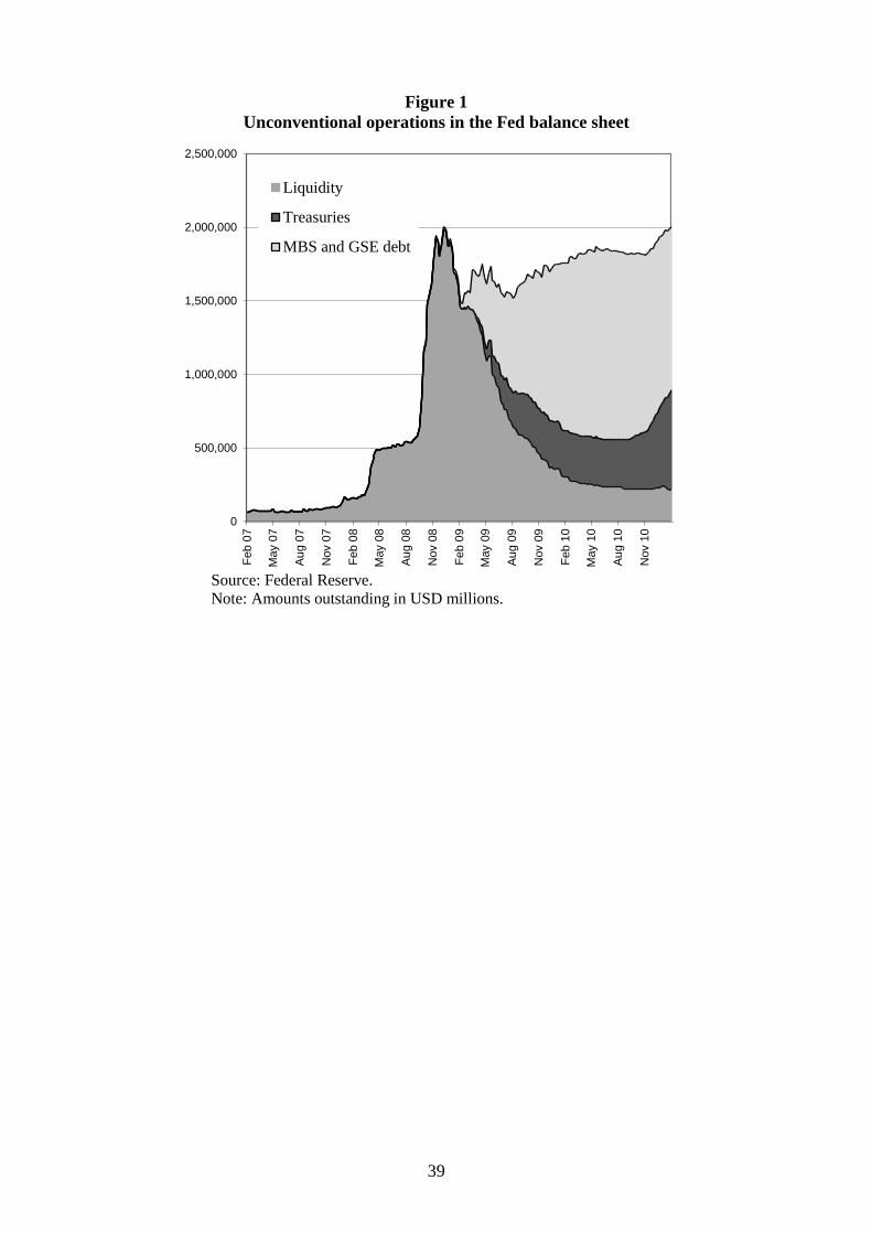
39

Figure 1 Unconventional operations in the Fed balance sheet

0

500,000

1,000,000

1,500,000

2,000,000

2,500,000

Feb

07

May

07

Aug

07

Nov

07

Feb

08

May

08

Aug

08

Nov

08

Feb

09

May

09

Aug

09

Nov

09

Feb

10

May

10

Aug

10

Nov

10

Liquidity

Treasuries

MBS and GSE debt

Source: Federal Reserve. Note: Amounts outstanding in USD millions.

40

Figure 2 Cumulated impact of US quantitative easing and other control variables

A - Equity portfolio flows

(In % of asset under management in country of destination)

United States

-20

-15

-10

-5

0

5

10

15

20

Mar-07 Sep-07 Mar-08 Sep-08 Mar-09 Sep-09 Mar-10 Sep-10

Other Factors

Monetary Policy

Actual

Emerging markets

-5

0

5

10

15

20

25

30

Mar-07 Sep-07 Mar-08 Sep-08 Mar-09 Sep-09 Mar-10 Sep-10

Other Factors

Monetary Policy

Actual

Advanced Economies

-25

-20

-15

-10

-5

0

5

Mar-07 Sep-07 Mar-08 Sep-08 Mar-09 Sep-09 Mar-10 Sep-10

Other Factors

Monetary Policy

Actual

41

Figure 2 (continued) Cumulated impact of US quantitative easing and other control variables

B - Bond portfolio flows

(In % of asset under management in country of destination)

United States

-20

-10

0

10

20

30

40

Mar-07 Sep-07 Mar-08 Sep-08 Mar-09 Sep-09 Mar-10 Sep-10

Other Factors

Monetary Policy

Actual

Emerging markets

-40

-30

-20

-10

0

10

20

30

40

50

Mar-07 Sep-07 Mar-08 Sep-08 Mar-09 Sep-09 Mar-10 Sep-10

Other Factors

Monetary Policy

Actual

Advanced Economies

-40

-35

-30

-25

-20

-15

-10

-5

0

5

10

Mar-07 Sep-07 Mar-08 Sep-08 Mar-09 Sep-09 Mar-10 Sep-10

Other Factors

Monetary Policy

Actual

42

Figure 2 (continued) Cumulated impact of US quantitative easing and other control variables

C – Equity prices

(Returns in %)

United States

-60

-50

-40

-30

-20

-10

0

10

20

30

40

Mar-07 Sep-07 Mar-08 Sep-08 Mar-09 Sep-09 Mar-10 Sep-10

Other Factors

Monetary Policy

Actual

Emerging markets

-50

-40

-30

-20

-10

0

10

20

30

Mar-07 Sep-07 Mar-08 Sep-08 Mar-09 Sep-09 Mar-10 Sep-10

Other Factors

Monetary Policy

Actual

Advanced Economies

-60

-50

-40

-30

-20

-10

0

10

20

30

Mar-07 Sep-07 Mar-08 Sep-08 Mar-09 Sep-09 Mar-10 Sep-10

Other Factors

Monetary Policy

Actual

43

Figure 2 (continued) Cumulated impact of US quantitative easing and other control variables

D – Bond yields

(Change in percentage points)

United States

-3

-2.5

-2

-1.5

-1

-0.5

0

0.5

1

Mar-07 Sep-07 Mar-08 Sep-08 Mar-09 Sep-09 Mar-10 Sep-10

Other Factors

Monetary Policy

Actual

Emerging markets

-2

-1

0

1

2

3

4

Mar-07 Sep-07 Mar-08 Sep-08 Mar-09 Sep-09 Mar-10 Sep-10

Other Factors

Monetary Policy

Actual

Advanced Economies

-2.5

-2

-1.5

-1

-0.5

0

0.5

1

1.5

2

2.5

Mar-07 Sep-07 Mar-08 Sep-08 Mar-09 Sep-09 Mar-10 Sep-10

Other Factors

Monetary Policy

Actual

44

Figure 2 (continued) Cumulated impact of US quantitative easing and other control variables

E – Exchange rate

(Returns in %)

United States

-15

-10

-5

0

5

10

15

Mar-07 Sep-07 Mar-08 Sep-08 Mar-09 Sep-09 Mar-10 Sep-10

Other Factors

Monetary Policy

Actual

Emerging markets

-10

-5

0

5

10

15

20

Mar-07 Sep-07 Mar-08 Sep-08 Mar-09 Sep-09 Mar-10 Sep-10

Other Factors

Monetary Policy

Actual

Advanced Economies

-20

-15

-10

-5

0

5

10

15

Mar-07 Sep-07 Mar-08 Sep-08 Mar-09 Sep-09 Mar-10 Sep-10

Other Factors

Monetary Policy

Actual

Note: The cumulated contributions of different explanatory variables are calculated according to the benchmark model in Tables 4-6.

45

Figure 3 Cyclicality of QE policies: correlation between the contribution of US quantitative easing and the

contribution of other control variables to portfolio flows

Equity Portfolio Flows

-.50

.5

01jul2008 01jan2009 01jul2009 01jan2010 01jul2010 01jan2011

United States Advanced EconomiesEmerging Markets

Bond Portfolio Flows

-.50

.5

01jul2008 01jan2009 01jul2009 01jan2010 01jul2010 01jan2011

United States Advanced EconomiesEmerging Markets

Note: the correlation is calculated over a twelve-month rolling window. Contributions of different explanatory variables are calculated according to the benchmark model in Table 4.

46

APPENDIX

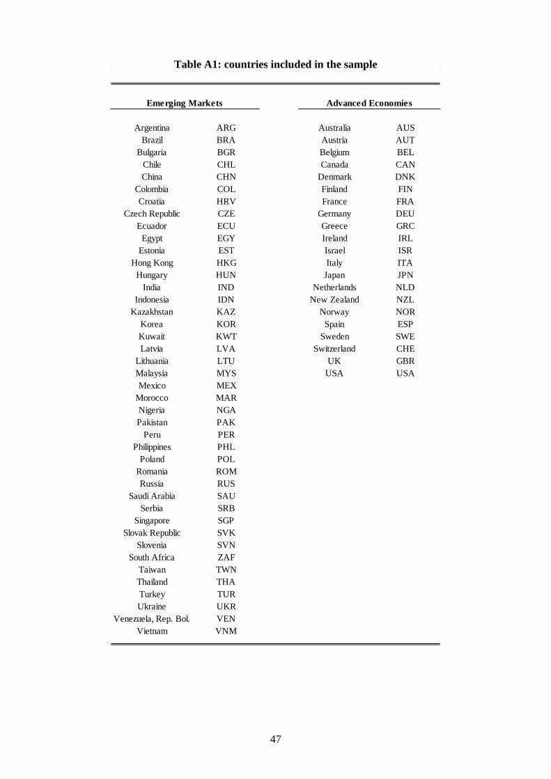
47

Table A1: countries included in the sample

Argentina ARG Australia AUSBrazil BRA Austria AUT

Bulgaria BGR Belgium BELChile CHL Canada CANChina CHN Denmark DNK

Colombia COL Finland FINCroatia HRV France FRA

Czech Republic CZE Germany DEUEcuador ECU Greece GRC

Egypt EGY Ireland IRLEstonia EST Israel ISR

Hong Kong HKG Italy ITAHungary HUN Japan JPN

India IND Netherlands NLDIndonesia IDN New Zealand NZL

Kazakhstan KAZ Norway NORKorea KOR Spain ESPKuwait KWT Sweden SWELatvia LVA Switzerland CHE

Lithuania LTU UK GBRMalaysia MYS USA USAMexico MEX

Morocco MARNigeria NGAPakistan PAK

Peru PERPhilippines PHL

Poland POLRomania ROMRussia RUS

Saudi Arabia SAUSerbia SRB

Singapore SGPSlovak Republic SVK

Slovenia SVNSouth Africa ZAF

Taiwan TWNThailand THATurkey TURUkraine UKR

Venezuela, Rep. Bol. VENVietnam VNM

Advanced EconomiesEmerging Markets

48

Table A2 – Stylized facts of QE announcements and asset prices

A. United States

QE 1 4.19 -0.34 -0.41QE 2 -4.94 -0.27 0.15QE 3 4.18 -0.33 -2.46QE 4 0.04 0.30 0.24QE 5 0.79 -0.40 -2.90QE 6 1.84 -0.11 -0.77QE 7 -1.96 -0.07 0.68QE 8 2.03 0.06 -0.52QE 9 -3.41 -0.15 1.16QE 10 0.19 0.05 0.18QE 11 0.93 0.01 0.34QE 12 2.30 -0.13 -0.70

QE I (1 to 5) 4.17 -1.04 *** -5.37 ***QE I (1,3,4,5) 9.15 ** -0.78 *** -5.52 ***QEII (9 to 12) -0.09 -0.21 1.02QEII (10,11,12) 3.36 -0.06 -0.15

Change in 10y yield

Change in S&P 500 Index

Change in NEER

B. Emerging Markets

QE 1 1.60 -0.18 -0.34QE 2 -2.03 -0.12 0.51QE 3 1.53 -0.06 -1.64QE 4 0.28 -0.04 0.63QE 5 1.52 -0.02 -1.52QE 6 0.88 0.02 -0.52QE 7 0.09 -0.04 0.18QE 8 1.21 -0.03 -0.61QE 9 -1.30 -0.04 0.99QE 10 0.56 -0.01 0.10QE 11 -0.05 0.01 0.29QE 12 1.33 -0.02 -0.57

QE I (1 to 5) 2.89 *** -0.69 ** -2.93 ***QE I (1,3,4,5) 5.07 *** -0.48 -3.52 ***QEII (9 to 12) 0.43 -0.08 0.93 **QEII (10,11,12) 1.86 *** -0.02 -0.25

Change in the local equity price index

Change in 10y yield

Change in FX USD

49

Table A2 (continued)

C. Advanced Economies

QE 1 1.26 -0.11 -0.24QE 2 -3.56 -0.15 0.37QE 3 0.75 -0.17 -4.30QE 4 0.94 -0.07 1.27QE 5 0.92 -0.12 -4.45QE 6 1.87 -0.01 -1.09QE 7 -1.12 -0.05 0.66QE 8 2.20 0.07 -0.98QE 9 -2.83 -0.02 2.08QE 10 0.83 0.01 0.04QE 11 0.00 0.02 0.41QE 12 0.69 0.00 -1.20

QE I (1 to 5) 0.28 -0.63 *** -7.65 ***QE I (1,3,4,5) 3.86 *** -0.48 *** -8.06 ***QEII (9 to 12) -1.33 0.02 1.47 ***QEII (10,11,12) 1.51 ** 0.04 -0.74 *

Change in the local equity price index

Change in 10y yield

Change in FX USD

Note: The upper part of the table shows the cumulated (two-day) impact of each announcement, i.e. the change of the dependent variable between the closing price on the day before the event (t-1) and the closing price on the day after the event (t+1). See Table 1 for the description of the events/announcements. The lower part of the table shows the total impact of different groups of announcements (with the impact of each of the announcements being cumulated over two days). The number in the parenthesis indicates the events included in the group. More specifically, the total impact for groups of announcements has been calculated using the following regression:

yt = c + β Dt + εt Where Dt is a dummy equal to (1 / N*2) on each of the N announcements in the group and on the following day. By constructing the dummy in this way, the coefficient β measures the total impact of the group of announcements. “***”, “**” and “*” indicate significance at the 1%, 5% and 10% confidence level respectively.

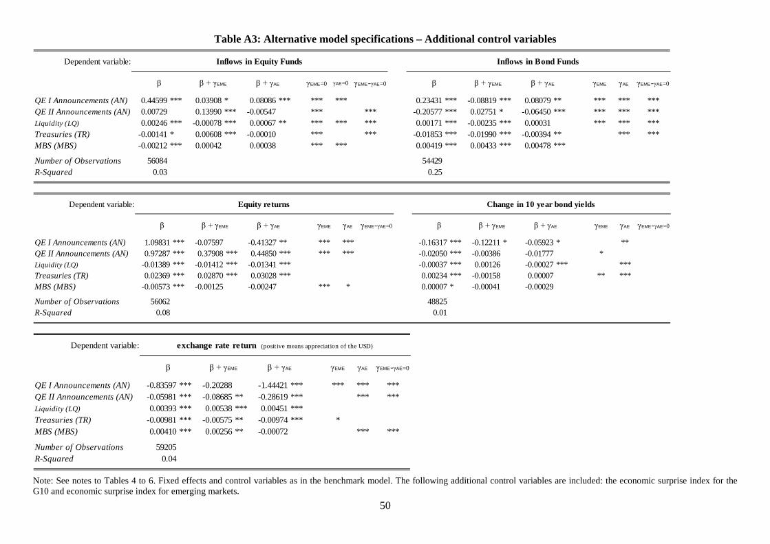
50

Table A3: Alternative model specifications – Additional control variables

Dependent variable:

γEME=0 γAE=0 γEME-γAE=0 γEME γAE γEME-γAE=0

QE I Announcements (AN) 0.44599 *** 0.03908 * 0.08086 *** *** *** 0.23431 *** -0.08819 *** 0.08079 ** *** *** ***QE II Announcements (AN) 0.00729 0.13990 *** -0.00547 *** *** -0.20577 *** 0.02751 * -0.06450 *** *** *** ***Liquidity (LQ) 0.00246 *** -0.00078 *** 0.00067 ** *** *** *** 0.00171 *** -0.00235 *** 0.00031 *** *** ***Treasuries (TR) -0.00141 * 0.00608 *** -0.00010 *** *** -0.01853 *** -0.01990 *** -0.00394 ** *** ***MBS (MBS) -0.00212 *** 0.00042 0.00038 *** *** 0.00419 *** 0.00433 *** 0.00478 ***

Number of Observations 56084 54429R-Squared 0.03 0.25

Inflows in Equity Funds Inflows in Bond Funds

β β + γEME β + γAE β β + γEME β + γAE

Dependent variable:

γEME γAE γEME-γAE=0 γEME γAE γEME-γAE=0

QE I Announcements (AN) 1.09831 *** -0.07597 -0.41327 ** *** *** -0.16317 *** -0.12211 * -0.05923 * **QE II Announcements (AN) 0.97287 *** 0.37908 *** 0.44850 *** *** *** -0.02050 *** -0.00386 -0.01777 *Liquidity (LQ) -0.01389 *** -0.01412 *** -0.01341 *** -0.00037 *** 0.00126 -0.00027 *** ***Treasuries (TR) 0.02369 *** 0.02870 *** 0.03028 *** 0.00234 *** -0.00158 0.00007 ** ***MBS (MBS) -0.00573 *** -0.00125 -0.00247 *** * 0.00007 * -0.00041 -0.00029

Number of Observations 56062 48825R-Squared 0.08 0.01

Equity returns Change in 10 year bond yields

β + γAEβ β + γEME β + γAE β β + γEME

Dependent variable:

γEME γAE γEME-γAE=0

QE I Announcements (AN) -0.83597 *** -0.20288 -1.44421 *** *** *** ***QE II Announcements (AN) -0.05981 *** -0.08685 ** -0.28619 *** *** ***Liquidity (LQ) 0.00393 *** 0.00538 *** 0.00451 ***Treasuries (TR) -0.00981 *** -0.00575 ** -0.00974 *** *MBS (MBS) 0.00410 *** 0.00256 ** -0.00072 *** ***

Number of Observations 59205R-Squared 0.04

exchange rate return (positive means appreciation of the USD)

β + γEME β + γAEβ

Note: See notes to Tables 4 to 6. Fixed effects and control variables as in the benchmark model. The following additional control variables are included: the economic surprise index for the G10 and economic surprise index for emerging markets.

51

Table A4: Alternative model specifications – Asymmetric impact of monetary policy operations

Dependent variable:

γEME=0 γAE=0 γEME-γAE=0 γEME γAE γEME-γAE=0

QE I Announcements (AN) 0.46195 *** 0.05162 ** 0.07466 *** *** *** 0.21529 *** -0.04644 *** 0.06145 * *** *** ***QE II Announcements (AN) 0.06052 *** 0.11795 *** 0.01711 *** *** *** -0.08788 *** 0.03080 *** -0.02903 *** *** **Liquidity (LQ) 0.00398 *** -0.00008 0.00267 *** *** *** *** 0.00560 *** -0.00223 *** 0.00313 *** *** *** ***Treasuries (TR) 0.00074 0.00246 ** -0.00230 ** ** -0.01411 *** -0.01747 *** -0.00560 *** *** *** ***MBS (MBS) -0.00300 *** 0.00133 ** 0.00042 *** *** 0.00187 *** 0.00440 *** 0.00441 *** *** ***

Number of Observations 56084 54429R-Squared 0..03 0.26

β + γAE

Inflows in Equity Funds Inflows in Bond Funds

β β + γEME β + γAE β β + γEME

Dependent variable:

γEME γAE γEME-γAE=0 γEME γAE γEME-γAE=0

QE I Announcements (AN) 1.32454 *** -0.02193 -0.31871 * *** *** -0.16043 *** -0.12578 -0.05603 **QE II Announcements (AN) 0.81252 *** 0.23950 * 0.31729 *** *** *** -0.02951 *** -0.00007 -0.02277 ***Liquidity (LQ) -0.02504 *** -0.01834 *** -0.01912 *** *** *** -0.00060 *** 0.00148 -0.00047 *** ***Treasuries (TR) 0.03665 *** 0.02619 *** 0.03222 *** 0.00192 *** -0.00163 -0.00002 **MBS (MBS) -0.00319 *** 0.00190 -0.00006 *** * 0.00026 *** -0.00045 -0.00022 *

Number of Observations 56062 48825R-Squared 0.08 0.01

β + γAEβ + γAE β β + γEMEβ β + γEME

Equity returns Change in 10 year bond yields

Dependent variable:

γEME γAE γEME-γAE=0

QE I Announcements (AN) -0.90001 *** -0.28432 ** -1.49625 *** *** *** ***QE II Announcements (AN) 0.02718 *** -0.00345 -0.12369 ** ** *Liquidity (LQ) 0.00696 *** 0.00911 *** 0.00829 ***Treasuries (TR) -0.00597 *** -0.00322 0.00294 *** *MBS (MBS) 0.00275 *** 0.00154 -0.00325 *** *** ***

Number of Observations 59205R-Squared 0.04

β β + γEME β + γAE

exchange rate return (positive means appreciation of the USD)

Note: See notes to Tables 4 to 6. Differentiation between expansionary and tightening monetary policy operations. Only the coefficients of expansionary monetary policy operations are reported; otherwise as in the benchmark model.

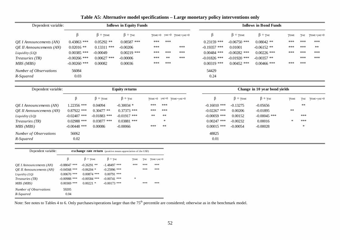
52

Table A5: Alternative model specifications – Large monetary policy interventions only

Dependent variable:

γEME=0 γAE=0 γEME-γAE=0 γEME γAE γEME-γAE=0

QE I Announcements (AN) 0.43863 *** 0.05292 ** 0.08587 *** *** *** 0.23159 *** -0.06750 *** 0.08042 ** *** *** ***QE II Announcements (AN) 0.02016 ** 0.13311 *** -0.00206 *** *** -0.19357 *** 0.01001 -0.06152 ** *** *** **Liquidity (LQ) 0.00385 *** -0.00049 0.00219 *** *** *** *** 0.00484 *** -0.00282 *** 0.00226 *** *** *** ***Treasuries (TR) -0.00266 *** 0.00627 *** -0.00006 *** ** *** -0.01826 *** -0.01920 *** -0.00357 ** *** ***MBS (MBS) -0.00260 *** 0.00082 0.00036 *** *** 0.00319 *** 0.00452 *** 0.00466 *** *** ***

Number of Observations 56084 54429R-Squared 0.03 0.24

Inflows in Equity Funds Inflows in Bond Funds

β β + γEME β + γAE β β + γEME β + γAE

Dependent variable:

γEME=0 γAE=0 γEME-γAE=0 γEME γAE γEME-γAE=0

QE I Announcements (AN) 1.22356 *** 0.04094 -0.30034 * *** *** -0.16010 *** -0.13275 -0.05656 **QE II Announcements (AN) 0.87922 *** 0.30477 ** 0.37373 *** *** *** -0.02267 *** 0.00206 -0.01895 **Liquidity (LQ) -0.02407 *** -0.01883 *** -0.01917 *** ** ** -0.00059 *** 0.00152 -0.00045 *** ***Treasuries (TR) 0.02988 *** 0.03877 *** 0.03881 *** * 0.00247 *** -0.00232 0.00016 * ***MBS (MBS) -0.00448 *** 0.00086 -0.00066 *** ** 0.00015 *** -0.00054 -0.00028 *

Number of Observations 56062 48825R-Squared 0.02 0.01

Equity returns Change in 10 year bond yields

β β + γEME β + γAE β β + γEME β + γAE

Dependent variable:

γEME γAE γEME-γAE=0

QE I Announcements (AN) -0.88047 *** -0.26291 ** -1.48497 *** *** *** ***QE II Announcements (AN) -0.04568 *** -0.06204 * -0.25996 *** *** ***Liquidity (LQ) 0.00670 *** 0.00874 *** 0.00791 ***Treasuries (TR) -0.00988 *** -0.00584 *** -0.00741 *** *MBS (MBS) 0.00369 *** 0.00221 * -0.00173 *** *** ***

Number of Observations 59205R-Squared 0.04

exchange rate return (positive means appreciation of the USD)

β β + γEME β + γAE

Note: See notes to Tables 4 to 6. Only purchases/operations larger than the 75th percentile are considered; otherwise as in the benchmark model.

53

Table A6: Alternative model specifications – Using daily data on Treasury bond purchases Dependent variable:

γEME=0 γAE=0 γEME-γAE=0 γEME γAE γEME-γAE=0

QE I Announcements (AN) 0.45090 *** 0.03829 * 0.08577 *** *** *** 0.25656 *** -0.06352 *** 0.08704 ** *** *** ***QE II Announcements (AN) 0.00720 0.11899 *** -0.01216 *** *** -0.16052 *** 0.07146 *** -0.04520 ** *** *** ***Liquidity (LQ) 0.00250 *** -0.00080 *** 0.00071 ** *** *** *** 0.00186 *** -0.00216 *** 0.00025 *** *** ***Treasuries (TR) 0.00047 0.00563 *** 0.00206 *** ** -0.00806 *** -0.00777 *** -0.00146 *** ***MBS (MBS) -0.00212 *** 0.00058 0.00040 *** *** 0.00388 *** 0.00401 *** 0.00482 *** *

Number of Observations 56084 54429R-Squared 0.03 0.25

β β + γEME β + γAE β β + γEME β + γAE

Inflows in Equity Funds Inflows in Bond Funds

Dependent variable:

γEME=0 γAE=0 γEME-γAE=0 γEME γAE γEME-γAE=0

QE I Announcements (AN) 1.05505 *** -0.11687 -0.44881 *** *** *** -0.16547 *** -0.12154 * -0.06097 * **QE II Announcements (AN) 0.92808 *** 0.30171 ** 0.34746 *** *** *** -0.02454 *** 0.00315 -0.01210 ***Liquidity (LQ) -0.01449 *** -0.01467 *** -0.01389 *** -0.00040 *** 0.00126 -0.00030 *** ***Treasuries (TR) 0.01016 *** 0.01796 *** 0.02363 *** ** *** 0.00106 *** -0.00168 -0.00130 ** *MBS (MBS) -0.00469 *** -0.00015 -0.00136 *** ** 0.00013 *** -0.00044 -0.00027 *

Number of Observations 56062 48825R-Squared 0.08 0.01

β β + γEME β + γAE β β + γEME β + γAE

Equity returns Change in 10 year bond yields

Dependent variable:

γEME γAE γEME-γAE=0

QE I Announcements (AN) -0.83306 *** -0.20115 -1.44111 *** *** *** ***QE II Announcements (AN) -0.05295 *** -0.09694 *** -0.28032 *** *** ***Liquidity (LQ) 0.00393 *** 0.00537 *** 0.00451 ***Treasuries (TR) -0.00260 *** 0.00154 -0.00237 ** *MBS (MBS) 0.00403 *** 0.00257 ** -0.00079 * *** ***

Number of Observations 59205R-Squared 0.04

β β + γEME β + γAE

exchange rate return (positive means appreciation of the USD)

Note: See notes to Tables 4 to 6. The weekly aggregate data on Treasury purchases are replaced with daily purchases data released by the New York Fed; otherwise as in the benchmark model.

54

Table A7: Alternative model specifications – bootstrapped standard errors

Dependent variable:

γEME=0 γAE=0 γEME-γAE=0 γEME γAE γEME-γAE=0

QE I Announcements (AN) 0.44599 ** 0.03908 * 0.08086 *** ** ** 0.23431 * -0.08819 *** 0.08079 ** ** ***QE II Announcements (AN) 0.00729 0.13990 *** -0.00547 *** *** -0.20577 ** 0.02751 ** -0.06450 ** ** ***Liquidity (LQ) 0.00246 ** -0.00078 *** 0.00067 ** *** *** 0.00171 -0.00235 *** 0.00031 *** ***Treasuries (TR) -0.00141 0.00608 *** -0.00010 ** *** -0.01853 *** -0.01990 *** -0.00394 ** ** ***MBS (MBS) -0.00212 0.00042 0.00038 * * 0.00419 *** 0.00433 *** 0.00478 ***

Number of Observations 56084 54429R-Squared 0.02 0.02

β β + γEME β + γAE β β + γEME β + γAE

Inflows in Equity Funds Inflows in Bond Funds

Dependent variable:

γEME γAE γEME-γAE=0 γEME γAE γEME-γAE=0

QE I Announcements (AN) 1.09831 * -0.07597 -0.41327 ** ** -0.16317 *** -0.12211 * -0.05923 *QE II Announcements (AN) 0.97287 *** 0.37908 *** 0.44850 *** ** ** -0.02050 * -0.00386 -0.01777Liquidity (LQ) -0.01389 *** -0.01412 *** -0.01341 *** -0.00037 0.00126 -0.00027 ***Treasuries (TR) 0.02369 *** 0.02870 *** 0.03028 *** 0.00234 -0.00158 0.00007 *MBS (MBS) -0.00573 ** -0.00125 -0.00247 * 0.00007 -0.00041 -0.00029

Number of Observations 56062 48825R-Squared 0.08 0.01

β β + γEME β + γAE β β + γEME β + γAE

Equity returns Change in 10 year bond yields

Dependent variable:

γEME γAE γEME-γAE=0

QE I Announcements (AN) -0.83597 ** -0.20288 -1.44421 *** ***QE II Announcements (AN) -0.05981 -0.08685 *** -0.28619 *** ** ***Liquidity (LQ) 0.00393 *** 0.00538 *** 0.00451 ***Treasuries (TR) -0.00981 *** -0.00575 ** -0.00974 ***MBS (MBS) 0.00410 ** 0.00256 ** -0.00072 *** ***

Number of Observations 59205R-Squared 0.04

β β + γEME β + γAE

exchange rate return (positive means appreciation of the USD)

Note: See notes to Tables 4 to 6. Standard errors are computed with a bootstrap; otherwise as in the benchmark model.

55

Table A8: Alternative model specifications – Differentiating between Treasury bond purchases during QE1 and QE2 Dependent variable:

γEME=0 γAE=0 γEME-γAE=0 γEME γAE γEME-γAE=0

QE I Announcements (AN) 0.46789 *** 0.05312 ** 0.10173 *** *** *** 0.32508 *** -0.03916 * 0.14477 *** *** *** ***QE II Announcements (AN) 0.00841 0.13789 *** -0.00480 *** *** -0.19686 *** 0.01567 -0.06546 *** *** *** ***Liquidity (LQ) 0.00269 *** -0.00062 * 0.00089 *** *** *** *** 0.00272 *** -0.00184 *** 0.00104 *** *** *** ***Treasuries QE1 (TR1) 0.00667 *** 0.01068 *** 0.00758 *** 0.01866 *** -0.00574 *** 0.02044 *** *** ***Treasuries QE2 (TR2) -0.00785 *** 0.00330 -0.00586 *** *** ** *** -0.04680 *** -0.02998 *** -0.02295 *** *** *** ***MBS (MBS) -0.00283 *** 0.00017 -0.00025 *** *** 0.00058 *** 0.00289 *** 0.00256 *** *** ***

Number of Observations 56084 54429R-Squared 0.03 0.26

Inflows in Equity Funds Inflows in Bond Funds

β β + γEME β + γAE β β + γEME β + γAE

Dependent variable:

γEME=0 γAE=0 γEME-γAE=0 γEME γAE γEME-γAE=0

QE I Announcements (AN) 1.10098 *** -0.04185 -0.35380 ** *** *** -0.16864 *** -0.12698 * -0.06532 * **QE II Announcements (AN) 0.96932 *** 0.38935 *** 0.47162 *** *** *** -0.02259 *** -0.00575 -0.02032 **Liquidity (LQ) -0.01392 *** -0.01377 *** -0.01277 *** -0.00042 *** 0.00121 -0.00033 *** **Treasuries QE1 (TR1) 0.03329 *** 0.05618 *** 0.07156 *** *** *** -0.00011 -0.00394 -0.00292 * *Treasuries QE2 (TR2) 0.03005 *** 0.02460 *** 0.01358 *** *** 0.00448 *** 0.00025 0.00242 *** *** *** **MBS (MBS) -0.00526 *** -0.00228 -0.00484 *** * 0.00035 *** -0.00020 -0.00001 **

Number of Observations 56062 48825R-Squared 0.08 0.01

Equity returns Change in 10 year bond yields

β β + γEME β + γAE β β + γEME β + γAE

Dependent variable:

γEME γAE γEME-γAE=0

QE I Announcements (AN) -0.86534 *** -0.23086 * -1.47200 *** *** *** ***QE II Announcements (AN) -0.06958 *** -0.09613 *** -0.29571 *** *** ***Liquidity (LQ) 0.00353 *** 0.00500 *** 0.00412 ***Treasuries QE1 (TR1) -0.02058 *** -0.01522 *** -0.01954 ***Treasuries QE2 (TR2) -0.00433 *** 0.00004 -0.00405 *MBS (MBS) 0.00509 *** 0.00354 *** 0.00022 *** **

Number of Observations 59205R-Squared 0.04

exchange rate return (positive means appreciation of the USD)

β β + γEME β + γAE

Note: See notes to Tables 4 to 6. Differentiation between Treasury bond purchases during QE1 (from March to October 2009) and QE2 (after August 2010); otherwise as in the benchmark model.

56

Table A9: Alternative model specifications – Two-stage approach

Dependent variable:

γEME=0 γAE=0 γEME-γAE=0 γEME γAE γEME-γAE=0

QE I Announcements (AN) 0.33987 *** 0.04072 0.14308 *** *** *** ** 0.16586 *** -0.14472 *** 0.08168 *** *** *** ***QE II Announcements (AN) -0.00025 0.11275 *** -0.01218 *** *** 0.02254 *** 0.06593 *** 0.01453 *Liquidity (LQ) 0.00135 *** -0.00157 ** -0.00007 *** *** * 0.00113 *** -0.00164 *** 0.00027 *** *** ***Treasuries QE1 (TR1) 0.00770 *** 0.00103 -0.00228 *** *** *** * 0.00308 *** -0.00356 *** -0.00078 *** *** ***Treasuries QE2 (TR2) -0.00485 *** 0.00163 -0.00598 *** *** *** -0.00947 *** -0.01886 *** -0.00694 *** *** ** ***MBS (MBS) -0.00100 *** 0.00124 ** -0.00078 ** *** *** -0.00076 *** -0.00349 *** -0.00291 *** *** ***

Number of Observations 52170 51219R-Squared 0.03 0.26

β β + γEME β + γAE β β + γEME β + γAE

Inflows in Equity Funds Inflows in Bond Funds

Dependent variable:

γEME=0 γAE=0 γEME-γAE=0 γEME γAE γEME-γAE=0

QE I Announcements (AN) 2.59958 *** 1.38245 *** 0.52458 ** *** *** *** -0.14493 *** -0.19244 * -0.20297 *QE II Announcements (AN) 1.11043 *** 0.56895 *** 0.41707 *** *** *** -0.01069 *** 0.03509 * 0.00480 **Liquidity (LQ) 0.00463 *** -0.00511 *** -0.00199 *** *** * 0.00029 * -0.00027 0.00017 *** *Treasuries QE1 (TR1) -0.00840 *** 0.00041 -0.00389 -0.00073 *** 0.00327 0.00809 ** *Treasuries QE2 (TR2) 0.01212 *** 0.02258 *** 0.01854 *** * ** 0.00031 *** 0.00051 0.00082 **MBS (MBS) 0.01897 *** 0.01154 *** 0.01901 *** *** ** -0.00027 *** -0.00053 -0.00022

Number of Observations 52170 45925R-Squared 0.01 0.01

β β + γEME β + γAE β β + γEME β + γAE

Equity returns Change in 10 year bond yields

Dependent variable:

γEME γAE γEME-γAE=0

QE I Announcements (AN) -0.51600 *** -0.25096 * -1.51473 *** *** ***QE II Announcements (AN) -0.03725 *** -0.09583 ** -0.25274 *** *** **Liquidity (LQ) 0.00197 *** 0.00238 *** 0.00374 *** ***Treasuries QE1 (TR1) 0.00187 *** 0.00899 ** -0.00082 * *Treasuries QE2 (TR2) -0.00196 *** -0.00097 -0.00222MBS (MBS) -0.00172 ** -0.00597 *** -0.00392 *** *

Number of Observations 55382R-Squared 0.07

β β + γEME β + γAE

exchange rate return (positive means appreciation of the USD)

Note: See notes to Tables 4 to 6. LQ, TR1 and MBS are the unexpected part of Fed interventions, i.e. the residual of a regression where the size of operations is explained by predetermined indicators of market tensions that are unaffected by the Fed interventions (see section 4.3 for details on the two stage approach); otherwise as in the benchmark model.

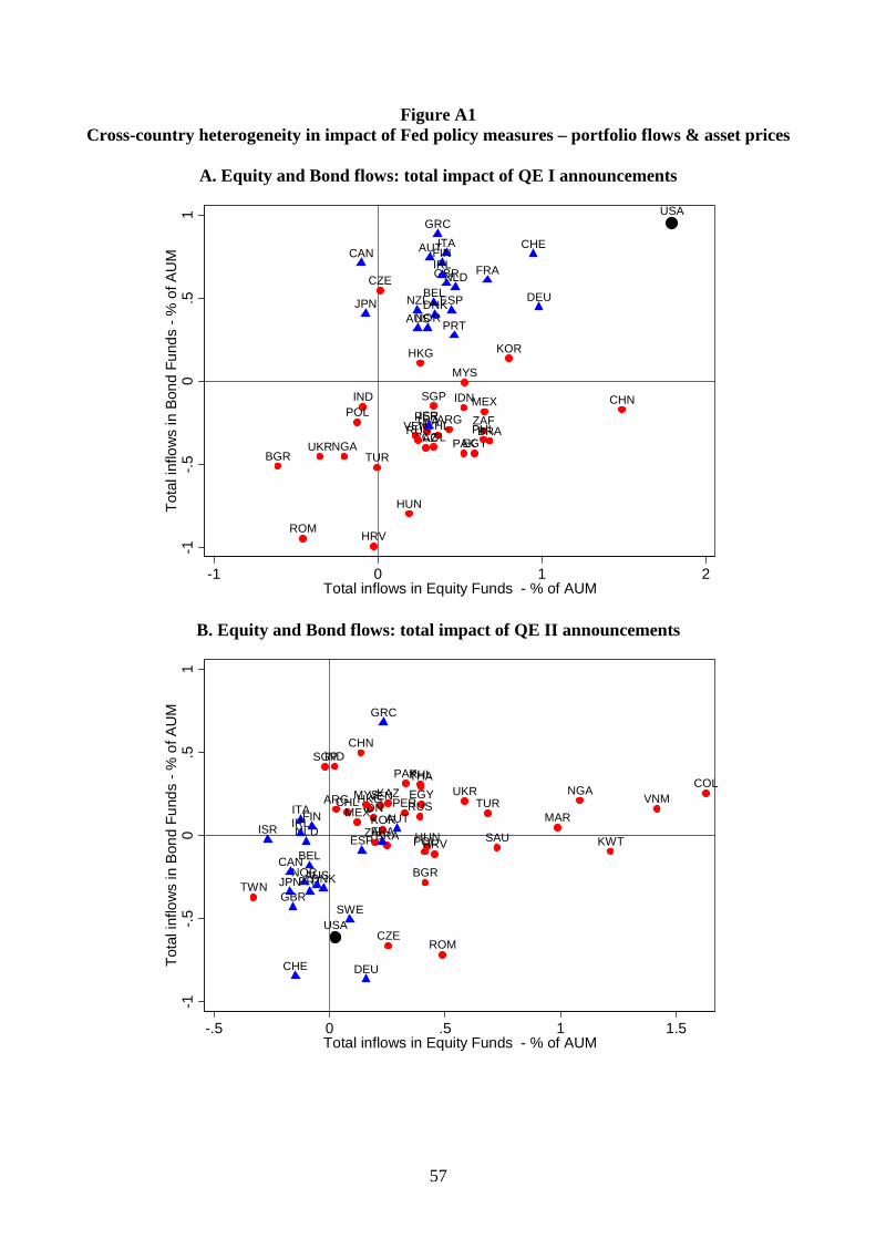
57

Figure A1 Cross-country heterogeneity in impact of Fed policy measures – portfolio flows & asset prices

A. Equity and Bond flows: total impact of QE I announcements

TUR

ZAFARGBRACHL

COL

MEXPER

VENEGY

HKG

IND IDN

KOR

MYS

PAKPHL

SGP

THA

NGAKAZ

BGR

RUS

CHN

UKR

CZE

HUN

HRV

POL

ROM

USA

GBR

AUT

BELDNK

FRA

DEU

ITA

NLD

NOR

CHECAN

JPN

FIN

GRC

IRL

PRT

ESPAUSNZL

ISR

-1-.5

0.5

1To

tal i

nflo

ws

in B

ond

Fund

s - %

of A

UM

-1 0 1 2Total inflows in Equity Funds - % of AUM

B. Equity and Bond flows: total impact of QE II announcements

TUR

ZAF

ARG

BRA

CHLCOL

MEXPERVEN

KWTSAU

EGY

TWN

HKG

IND

IDNKOR

MYS

PAKPHLSGP

THA

VNMMAR

NGAKAZ

BGR

RUS

CHN

UKR

CZE

HUNHRVPOL

ROM

USA

GBR

AUT

BEL

DNK

FRA

DEU

ITA

NLD

NOR

SWE

CHE

CAN

JPN

FIN

GRC

IRL

PRT

ESP

AUS

ISR

-1-.5

0.5

1To

tal i

nflo

ws

in B

ond

Fund

s - %

of A

UM

-.5 0 .5 1 1.5Total inflows in Equity Funds - % of AUM

58

C. Equity and Bond flows: Impact of treasury purchases at the maximum expansion of the programme

TUR

ZAFARG

BRA

CHLCOL

MEXPERVEN

KWT

SAU EGY

TWN

HKGIND

IDN

KORMYS

PAKPHL

SGPTHA

MAR

NGAKAZ

BGR

RUS

CHN

UKR

CZEHUN

HRV

POL

ROM

USA

GBR

AUT

BELDNK

FRA

DEU

ITANLD

NOR

SWECHE

CAN

JPN

FIN

GRC

IRL

PRT

ESP

AUS

NZL

ISR

-20

-10

010

Tota

l inf

low

s in

Bon

d Fu

nds

- % o

f AU

M

-10 -5 0 5 10Total inflows in Equity Funds - % of AUM

Note: Figures A to C show the total impact of QE instruments. The total impact is calculated by multiplying the estimated impact coefficient of a QE instrument by the total size of the QE programme. Underlying coefficients are estimated with modified version of the benchmark model, where the coefficients measuring the impact of QE instruments are country-specific

59

Figure A2 Cross-country heterogeneity in impact of Fed policy measures – asset prices

A. Equity prices and Bond yields: total impact of QE I announcements

ZAF

BRA

CHL

COL

MEX

SAU

TWN

HKG

INDKOR

MYS

PHL

SGP

THA

BGR

RUS

CHNCZE

POL

USA

GBR AUT

BEL

DNK FRADEU

ITANLDNOR

SWE

CHE

CAN

JPN

FIN

GRCIRL PRT

ESP

AUS

NZL

ISR

-1-.5

0.5

Tota

l yie

ld c

hang

e

-10 -5 0 5 10Total equity price change

B. Equity prices and Bond yields: total impact of QE II announcements

TUR

ZAF

ARG

BRA

COL

MEX

VEN

TWN

HKG

IND

IDN

KOR

MYS

PHL

SGP

THA

VNMNGA

BGR

RUS

CHN

CZE

HUN

HRV

POL

USA

GBR

AUTBELDNK FRA

DEU

ITA

NLD

SWE

CHE

CAN

JPN

FIN

GRC

IRL

PRT

ESP

AUS

NZL

ISR

-.20

.2.4

Tota

l yie

ld c

hang

e

-4 -2 0 2 4 6Total equity price change

60

C. Equity prices and Bond yields: Impact of treasury purchases at the maximum expansion of the programme

TUR

ZAF

BRA

CHL

COL

MEX

VEN

SAU

TWNHKG

INDIDN

KOR

MYS

PHL

SGP

THA

VNM

NGA

BGR

RUSCHN

CZE

HUN

HRV

POL

USA

GBRAUTBEL

DNK

FRA

DEU

ITA

NLDNOR SWE

CHECANJPN

FIN

GRC

IRL

PRT

ESP

AUSNZL

ISR

-3-2

-10

12

Tota

l yie

ld c

hang

e

-20 0 20 40 60Total equity price change

Note: See note to Figure A1.

61

Figure A3 Cross-country heterogeneity in impact of Fed policy measures – exchange rates

A. Exchange rate (total USD appreciation in %): total impact of QE I announcements

-10

-50

510

AU

SC

AN

CH

ED

NK

EU

RG

BR ISR

JPN

NO

RN

ZLS

WE

US

AA

RE

AR

GB

GR

BR

AC

HL

CH

NC

OL

CZE

EC

UE

GY

HK

GH

RV

HU

NID

NIN

DK

AZK

OR

KW

TM

AR

ME

XM

YS

NG

AP

AKP

ER PH

LP

OL

QAT

RO

MR

US

SAU

SG

PS

RB

THA

TUN

TUR

TWN

UK

RV

ENV

NM

ZAF

B. Exchange rate (total USD appreciation in %): total impact of QE II announcements

-4-2

02

AU

SC

AN

CH

ED

NK

EU

RG

BR ISR

JPN

NO

RN

ZLS

WE

US

AA

RE

AR

GB

GR

BR

AC

HL

CH

NC

OL

CZE

EC

UE

GY

HK

GH

RV

HU

NID

NIN

DK

AZK

OR

KW

TM

AR

ME

XM

YS

NG

AP

AKP

ER PH

LP

OL

QAT

RO

MR

US

SAU

SG

PS

RB

THA

TUN

TUR

TWN

UK

RV

ENV

NM

ZAF

62

C. Exchange rate (total USD appreciation in %): Impact of liquidity operations at the maximum expansion of the programme

-10

010

2030

40

AU

SC

AN

CH

ED

NK

EU

RG

BR ISR

JPN

NO

RN

ZLS

WE

US

AA

RE

AR

GB

GR

BR

AC

HL

CH

NC

OL

CZE

EC

UE

GY

HK

GH

RV

HU

NID

NIN

DK

AZK

OR

KW

TM

AR

ME

XM

YS

NG

AP

AKP

ER PH

LP

OL

QAT

RO

MR

US

SAU

SG

PS

RB

THA

TUN

TUR

TWN

UK

RV

ENV

NM

ZAF

D. Exchange rate (total USD appreciation in %): Impact of treasury purchases at the

maximum expansion of the programme

-20

-10

010

20

AU

SC

AN

CH

ED

NK

EU

RG

BR ISR

JPN

NO

RN

ZLS

WE

US

AA

RE

AR

GB

GR

BR

AC

HL

CH

NC

OL

CZE

EC

UE

GY

HK

GH

RV

HU

NID

NIN

DK

AZK

OR

KW

TM

AR

ME

XM

YS

NG

AP

AKP

ER PH

LP

OL

QAT

RO

MR

US

SAU

SG

PS

RB

THA

TUN

TUR

TWN

UK

RV

ENV

NM

ZAF

Note: See note to Figure A1.