Working Paper Series - European Central Bank · Working Paper Series . Real exchange rate...

Working Paper Series Real exchange rate misalignments in the euro area

Michael Fidora, Claire Giordano, Martin Schmitz

Disclaimer: This paper should not be reported as representing the views of the European Central Bank (ECB). The views expressed are those of the authors and do not necessarily reflect those of the ECB.

No 2108 / November 2017

Abstract

Building upon a Behavioural Equilibrium Exchange Rate (BEER) model, estimated at a quarterly frequency since 1999 on a broad sample of 57 countries, this paper assesses whether both the size and the persistence of real effective exchange rate misalignments from the levels implied by economic fundamentals are affected by the adoption of a single currency. While real misalignments are found to be smaller in the euro area than in its main trading partners, they are also more persistent, although the reactivity of real exchange rates to past misalignments increased, and therefore the persistence decreased, after the global financial crisis. In the absence of the nominal adjustment channel, an improvement in the quality of regulation and institutions is found to reduce the persistence of real exchange rate misalignments, plausibly by removing real rigidities.

Keywords: real effective exchange rate, equilibrium exchange rate, monetary union, regulation JEL codes: E24, E30, F00.

ECB Working Paper 2108, November 2017 1

Non-technical summary

This paper assesses whether both the size and the persistence of real exchange rate misalignments

from the levels implied by economic fundamentals are affected by the adoption of a single currency.

In order to do so, this paper provides estimates of exchange rate misalignments based on a reduced-

form relationship between real exchange rates and key macroeconomic fundamentals since 1999 at a

quarterly frequency for 57 euro and non-euro area countries, a so-called Behavioural Equilibrium

Exchange Rate model. In the medium run, real exchange rates should move back towards their

estimated equilibrium, thereby annulling any currency misalignment. However, significant

misalignments may persist if there are nominal or structural rigidities which hinder adjustment. This

paper therefore assesses whether the adoption of a single currency in the euro area, by introducing a

nominal rigidity in the form of fixed exchange rates, has spurred real currency misalignments. This is

ultimately an empirical issue, since the theoretical literature is inconclusive on the topic.

Our main findings are the following. First, real misalignments within the euro area are found to be

smaller than those of other advanced countries or of emerging economies, suggesting that the removal

of the nominal adjustment channel is not necessarily conducive to larger misalignments; to the

contrary, it can, for example, shield real effective exchange rates from the volatility stemming from

financial markets, thereby curbing the size of real disequilibria. Second, the reactivity of real

exchange rates to past misalignments within the euro area has been smaller than in other countries,

suggesting more persistent misalignments. Since 2009, however, the persistence of real misalignments

in euro area countries has decreased. Third, we find that better-quality regulation and institutions

increase the sensitivity of real effective exchange rates to past disequilibria, thus reducing their

persistence, plausibly by lowering the extent of real rigidities in the economy, which hinder the

adjustment process especially in countries, such as the euro area economies, which have given up the

nominal adjustment channel.


1 Introduction

An economy’s price or cost competitiveness is commonly measured by the real effective exchange

rate (REER). For euro area countries the ECB (Schmitz et al. 2012) calculates and publishes

Harmonised Competitiveness Indicators (HCIs), which are conceptually equivalent to REERs. The

REER is calculated as a weighted geometric average of the nominal exchange rates of a country vis-à-

vis the currencies of its main trading partners, deflated by relative prices or costs. These deflators are

expressed as indices rather than as levels, providing information solely on price competitiveness

dynamics. In order to appraise a country’s competitiveness position it is therefore preferable to assess

the REER’s distance from its benchmark, or equilibrium, level. The challenge is to construct a

suitable yardstick against which to appraise a country’s price-competitiveness performance.

Based on a Behavioural Equilibrium Exchange Rate (BEER) model, in the spirit of Clark and

MacDonald (1998), we specifically account for the structural determinants of real exchange rates

(RERs). In particular, we estimate a reduced-form relationship between RERs and key

macroeconomic fundamentals since 1999 at a quarterly frequency for 57 euro and non-euro area

countries, a vast sample when compared with the existing literature. This allows us to derive RER and

REER equilibrium values, as well as to compute the corresponding misalignments. Previous

contributions to this strand of the literature, amongst many applications, include Maeso Fernández,

Osbat and Schnatz (2001, 2004), Schnatz, Vijselaar and Osbat (2003), Lane and Milesi-Ferretti

(2004), Ricci, Milesi-Ferretti and Lee (2008) and Bussière et al. (2010).

In the medium run, real exchange rates should move in the direction of their equilibrium, thereby

annulling any currency misalignment, although significant deviations of REERs from their

equilibrium may persist if there are nominal or structural rigidities which hinder adjustment. We

indeed find evidence of significant REER misalignments in the countries under study. In particular,

we assess whether the adoption of a single currency in the euro area, by introducing a nominal rigidity

in the form of fixed exchange rates, has spurred real currency misalignments. Thereby, this paper

contributes to the open debate on the effect of flexible vs. fixed exchange rate regimes on the size and

persistence of real currency misalignments, starting with Friedman (1953), as well as to the literature

on inflation differentials and the persistence of inflation within the euro area (see, e.g., Altissimo,

Ehrmann and Smets, 2006; Angeloni and Ehrmann, 2007; de Haan, 2010). Moreover, this paper

explores the link between institutions and real exchange rate adjustment, contributing to the

surprisingly scanty literature on the topic (see, amongst others, Nouira and Sekkat, 2015).

Our main findings are the following. First, misalignments within the euro area are found to be smaller

than those of other advanced countries or of emerging economies, suggesting that the removal of the

nominal adjustment channel is not necessarily conducive to larger misalignments. Second, the

reactivity of REERs to past misalignments within the euro area has been slower than in other

countries, suggesting more persistent misalignments, but only in the period prior to 2009. Third, we

find that better-quality regulation and institutions increase the sensitivity of REERs to past


disequilibria, plausibly by reducing both the degree of “tolerance” towards REER disequilibria and

the extent of real rigidities in the economy.

The structure of the paper is the following. Section 2 briefly outlines the theoretical and empirical

debate on the links between a country’s exchange rate arrangement, on the one hand, and the size and

persistence of real exchange rate misalignments, on the other. Section 3 describes the specification of

the BEER model, as well as the dataset employed; next, it reviews the estimation technique and

provides estimation results. Section 4 examines the magnitude of estimated REER misalignments for

various country groupings under different nominal exchange rate regimes; it then compares the

persistence of REERs within the euro area to that of other countries, and explores the role of

regulation and institutional quality. Section 5 draws up some conclusions.

2 Exchange rate regimes and real exchange rate misalignments

From a theoretical standpoint, the relationship between exchange rate regimes and real currency

disequilibria is ambiguous. According to Friedman (1953), flexible exchange rates promote cross-

country price convergence even when prices of goods are sticky, since nominal exchange rate

fluctuations can substitute for nominal price adjustments when nominal prices are rigid.1 Moreover, as

price convergence can be achieved through currency trade in the foreign exchange market that

induces the nominal exchange rate to adjust, the flexibility of nominal exchange rates may be crucial

for the attainment of purchasing power parity (PPP). On the other hand, fixed exchange rates lower

transaction costs and foster cross-border trade in the goods market, thereby increasing the

transparency of price differentials that could be arbitraged away, and hence induce faster price

convergence (Rose, 2000). Furthermore, since capital markets are open in most countries, the price of

foreign exchange is not only the price that balances supply and demand for traded goods, but also an

asset price which reflects expectations of future fundamentals and risk premia. In this respect, Flood

and Rose (1999) develop a theoretical model that assumes that exchange rates are more volatile than

macroeconomic fundamentals and regards asset market shocks as the dominant factor driving volatile

exchange rate fluctuations when exchange rates are flexible. The elimination of flexibility in the

nominal exchange rate might therefore remove a source of destabilising shocks which lead to large

and persistent relative price deviations (see, e.g., the empirical analyses in Engel and Rogers, 2004;

Berka, Devereux and Engel, 2014; Bergin, Glick and Wu, 2017).

In the empirical literature no consensus on which type of exchange rate regime is more conducive to

smaller real misalignments has been reached either. Some analyses confirm that REERs can be largely

misaligned, irrespective of the exchange rate regime (see, e.g., Coudert, Couharde and Mignon, 2013).

1 This claim holds under at least two strong assumptions: first, final users of imported goods, in particular consumers, faceprices that are fully flexible in their own currency, since they adjust instantaneously to changes in nominal exchange rates,vis-à-vis sticky prices in the exporter’s currency (i.e. the currency in which exports are invoiced). Second, capital isimmobile across countries so that demand for foreign currency only arises to pay for imported goods (see Berka, Devereuxand Engel, 2012 for a deeper discussion of these assumptions).


Dubas (2009) instead points to larger misalignments under flexible exchange rate regimes in emerging

economies, whereas Coudert and Couharde (2009) and Holtemöller and Mallick (2013) show that

misalignments are larger when the currencies of emerging economies are pegged. The empirical

evidence is ambiguous not only concerning the size, but also the persistence of misalignments.

Indeed, the speed of mean-reversion of REERs to their equilibria has been found to be faster,

comparable or slower in fixed vs. flexible nominal exchange rate regimes, with no dominant result.

The empirical strategies adopted to analyse the issue of persistence have been mainly two-fold. On the

one hand, historical regime-switching events have been exploited to account for differences in the

speed of adjustment of REERs: studies have focused on a sample of advanced economies in the pre-

and post-Bretton Woods periods (Bergin, Glick and Wu, 2012) or on a number of euro area countries

before and after the introduction of the single currency (Huang and Yang, 2015; Bergin, Glick and

Wu 2017). An alternative empirical approach has been to explore the persistence of misalignments in

countries with different exchange rate arrangements within the same sample period, as in Mussa

(1986), Parsley and Popper (2001), Bissoondeeal (2008) and Berka, Devereux and Engel (2012).

Owing to the time-span considered in this paper (focused on the post-1999 period, due to data

availability), compensated by the vast country sample underlying our model, which includes both euro

and non-euro area countries, we mainly adopt this second empirical strategy and assess differences in

the size and persistence of misalignments between euro area countries and the other countries in our

sample.

One disadvantage of this approach is that country heterogeneity usually has important implications

not only on the exchange rate arrangement adopted but also on the speed of correction, and failure to

take account of these conditions will result in a spurious relationship between the exchange rate

arrangement and the speed of exchange rate adjustment (Huang and Yang, 2015). By controlling for

country-specific changes in economic fundamentals as well as for country fixed effects, we partially

overcome this drawback.2 Moreover, we test for the role of regulation and institutions in affecting the

sensitivity of REER movements to past misalignments, so as to investigate alternative channels of

adjustment other than the nominal exchange rate. Therefore, this paper also contributes to a strand of

the literature which is concerned with the link between institutions and exchange rate regimes (see,

e.g., Rodrik, 2008; Nouira and Sekkat, 2015; Franks et al., 2017).

3 A Behavioural Equilibrium Exchange Rate model

3.1 The structure of the BEER model

Abstracting from transaction costs, foreign trade and arbitrage in integrated and perfect-competition

goods markets should ensure that the law of one price (i.e. absolute PPP) holds for any good i so that

2 Huan and Yang (2015) mention the example of low-income countries which tend to impose higher tariffs to protect theirdomestic industries and are at the same time more prone to fixed exchange rate regimes. We indeed explicitly control fortrade openness, thereby attenuating this potential issue.


the price of good i should be the same across countries when converted into a common currency. Real

exchange rates should therefore be equal to zero in logarithms:

(1) 𝑝𝑝𝑡𝑡,𝑖𝑖 = 𝑝𝑝𝑡𝑡,𝑖𝑖∗ + 𝑒𝑒𝑡𝑡 => 𝑟𝑟𝑒𝑒𝑟𝑟𝑡𝑡,𝑖𝑖 = 𝑝𝑝𝑡𝑡,𝑖𝑖 − 𝑝𝑝𝑡𝑡,𝑖𝑖

∗ − 𝑒𝑒𝑡𝑡 = 0

where, at time t, 𝑝𝑝𝑡𝑡,𝑖𝑖 (𝑝𝑝𝑡𝑡,𝑖𝑖∗ ) is the log of the domestic-currency (foreign-currency) price of good i and

𝑒𝑒𝑡𝑡 and 𝑟𝑟𝑒𝑒𝑟𝑟𝑡𝑡,𝑖𝑖 are the logs of the nominal exchange rate and the real exchange rate of the domestic

currency relative to the foreign currency referring to good i.

If absolute PPP holds for individual goods, it holds also for any identical basket of goods. However, if

countries have different consumption baskets with weights and mixes of goods varying across

economies, then PPP does not hold anymore. In order to allow for a constant price differential

between baskets, the empirical literature has thus generally focused on relative PPP, that is:

(2) 𝑝𝑝𝑡𝑡 = 𝑝𝑝𝑡𝑡∗ + 𝑒𝑒𝑡𝑡 + 𝜃𝜃 => 𝑟𝑟𝑒𝑒𝑟𝑟𝑡𝑡 = 𝑝𝑝𝑡𝑡 − 𝑝𝑝𝑡𝑡∗ − 𝑒𝑒𝑡𝑡 = 𝜃𝜃

where 𝑝𝑝𝑡𝑡 (𝑝𝑝𝑡𝑡 ∗ ) is the log of the domestic-currency (foreign-currency) prices of a basket of goods, 𝑟𝑟𝑒𝑒𝑟𝑟𝑡𝑡

is the real exchange rate of the domestic currency relative to the foreign currency and 𝜃𝜃 is a constant

that reflects the differences in consumption basket composition across the two countries. The notion

of relative PPP thus assumes that real exchange rates are stationary, that is mean-reverting in the long-

run. Empirically, however, there is ample evidence of systematic deviations from both absolute and

relative PPP (see, e.g., Imbs et al.; 2002, Kilian and Zha, 2002; Taylor and Taylor, 2004; Taylor,

2006), leading to the well-known “PPP puzzle” (Rogoff, 1996). The traditional findings of Meese and

Rogoff (1983a) on the unpredictability of exchange rates at short horizons are generally undisputed,

and thus the empirical literature has converged toward explaining the behaviour of real exchange rates

at medium or long-term horizons. Amongst various empirical approaches, BEER models attempt to

explain the documented time-varying deviations from PPP at the latter horizons by modelling RERs

or REERs as a function of economic fundamentals.3

3 Differently from the BEER approach, alternative empirical approaches to estimating the determinants of real exchangerates are generally normative and include the following. The natural real exchange rate (NATREX) approach, originallyformulated by Stein (1990), defines the “natural” RER as the RER that ensures the equilibrium of the balance of payments inthe absence of cyclical factors, speculative capital movements and changes in international reserves. The NATREXguarantees both the internal and the external equilibrium in the long run: the internal equilibrium is achieved when thecapacity utilization rate is at its stationary mean; the external equilibrium is obtained when the balance of payments is inequilibrium in the long run, i.e. at the given exchange rate, investors are indifferent between holding domestic or foreignassets and the surplus of national investment relative to national savings is entirely financed through long-term borrowing.Although there are some attempts to measure the structural model underlying NATREX (see, for example, Gandolfo andFelettigh, 1998;Siregar and Rajan, 2006), this approach often boils down to estimating a reduced-form equation andtherefore, as noted by Stein (2001), the main difference between the BEER and the NATREX models is only that the latter,differently from the former, is theoretically grounded on a dynamic stock-flow model. Another class of models is theFundamental Equilibrium Exchange Rate (FEER) approach, advocated by Wren-Lewis (1992) and Williamson (1994). In itsmost popular applications (Isard, 2007; Lee et al., 2008; Cline and Williamson, 2010), the FEER approach is based on thecomputation of the required exchange rate adjustment to close the gap between the cyclically-adjusted current account andthe “current account norm”, which represents an optimal and sustainable value of the current account over a medium-termhorizon. The norm is either set in a normative manner or is derived from reduced-form regressions that estimate anequilibrium relationship between the current account and a set of plausible economic fundamentals that influence theinvestment-savings ratio. The calibration of the change in the exchange rate necessary to close the current account gap isbased on some additional assumptions about the exchange-rate pass-through coefficients and the price elasticities of exportsand imports. The magnitude of the required exchange rate adjustment crucially hinges on the accuracy of the estimation ofthe current account gap and on the measurement of the trade elasticities. In sum though, no “optimal” REER model has beenfound, although the issue has been heatedly debated (e.g. Cheung, Chinn and Fujii, 2010; Schnatz, 2011), also in connection


We estimate a BEER model in which the dependent variable (rer) is the bilateral RER of each

currency relative to a numéraire currency, for which we choose the euro, defined in such way that an

increase corresponds to an appreciation.4 The estimated elasticities are then employed to derive

equilibrium rates implied by economic fundamentals, against which actual bilateral RERs may be

appraised. Finally, we aggregate (equilibrium and actual) bilateral RERs into (equilibrium and actual)

REERs based on the trade weights used by the ECB to compute its official REERs and HCIs.

Similarly to Clark and MacDonald (1998), we start from the basic concept of uncovered real interest

parity (neglecting risk premia):

(3) 𝐸𝐸𝑡𝑡(𝑟𝑟𝑒𝑒𝑟𝑟𝑡𝑡+1) − 𝑟𝑟𝑒𝑒𝑟𝑟𝑡𝑡 = −(𝑟𝑟𝑡𝑡 − 𝑟𝑟𝑡𝑡∗) => 𝑟𝑟𝑒𝑒𝑟𝑟𝑡𝑡 = 𝐸𝐸𝑡𝑡(𝑟𝑟𝑒𝑒𝑟𝑟𝑡𝑡+1) + (𝑟𝑟𝑡𝑡 − 𝑟𝑟𝑡𝑡∗)

where 𝑟𝑟𝑡𝑡 and 𝑟𝑟𝑡𝑡∗ are the domestic and foreign real interest rates and 𝐸𝐸𝑡𝑡 denotes the expected value at

time t. By rearranging the terms in equation (3), the observed RER in time t is thus a positive function

of both the expected value of the RER in the following period and of the current real interest rate

differential defined as above. Clark and MacDonald (1998) assume that the unobservable expected

value of the RER is determined by a vector of long-run economic fundamentals, so the actual RER

depends both on the latter macroeconomic variables and on the real interest rate differential.

The BEER specification then incorporates economic fundamentals suggested by different theoretical

frameworks. Table B1 in Annex B provides an overview of the explanatory variables employed in

recent BEER model studies. In order to select the relevant economic fundamentals, we adopt a

general-to-specific approach, in which we keep all variables, suggested by the economic theory

literature, that are statistically significant at least at a 10 percent confidence level in most

specifications (which, as we shall see, differ according to the deflator used to construct the dependent

variable, the bilateral RER).5

One of the most popular explanations of the deviations from (absolute) PPP is due to Balassa (1964)

and Samuelson (1964). The two scholars posited that relative prices of non-traded and traded goods

are inversely related to the relative productivity in the two sectors, assuming free labour mobility

across sectors and tradable goods prices that are determined in the global market. In particular, a rise

in productivity in the tradable sector entails an increase in wages in the tradable sector, yet also bids

up wages in the non-tradable sector, without however a corresponding rise in productivity. This leads

to a higher general price level, which in turn implies a real appreciation in the currency. In order to

empirically investigate the Balassa-Samuelson effect, sector-specific productivities should be

with exchange-rate forecasting (see, for example, Meese and Rogoff, 1983a, 1983b; Gandolfo, Padoan and de Arcangelis,1993; Cheung et al., 2017).4 Using bilateral exchange rates as the dependent variable, instead of REERs as in some of the literature, has the advantagethat the former capture relative prices in a cleaner fashion in that, unlike REERs, they are unaffected by changes in tradeweights (Adler and Grisse, 2014). At the same time, the approach ensures the multilateral consistency of estimatedmisalignments given that the effective misalignments of each currency can be calculated as a weighted averagemisalignment of its bilateral exchange rates.5 In such an exercise, as in all BEER models, the economic fundamental variables cannot be interpreted to exhibit a causaleffect on RERs. Nonetheless, this approach can help determine the extent to which RERs diverge from their historical linkwith economic fundamentals.


employed.6 However, when productivity growth in the non-tradables sector is constant across

countries, which is a reasonable approximation as it is generally close to zero, aggregate labour

productivity measures may be employed, as shown in the simplified formalization of the Balassa-

Samuelson model in Annex A. Since the BEER model is estimated at a quarterly frequency for a large

set of countries, owing to data availability, we are constrained to employ aggregate, as opposed to

sectorial, measures. Using GDP per capita as a proxy of productivity to measure the Balassa-

Samuelson hypothesis – as is often done in the literature for a dearth of data on employment – implies

introducing an additional strong assumption of a stable labour participation rate, absent in the case of

using actual productivity measures. We therefore adopt two alternative measures of total-economy

productivity differentials, either relative productivity per employee or relative GDP per capita (which

in both cases we will refer to as relprod), in order to investigate any significant differences across the

two measures. In this respect, we follow Schnatz, Vijselaar and Osbat (2003) and Bénassy-Queré,

Béreau and Mignon (2009), which are the few studies that, to our knowledge, have similarly tested for

alternative proxies of the Balassa-Samuelson effect.

Whereas the Balassa-Samuelson model assumes that the REER depends entirely on supply factors,

demand-side variables that may impinge on the equilibrium exchange rate through time are also

typically considered, based on the observation that, in contrast to the assumptions underlying the

Balassa-Samuelson model, labour is not necessarily mobile across sectors in the short run. First,

openness to trade (relopen), i.e. the sum of exports and imports as a share of GDP, is used as a proxy

of the intensity of trade restrictions, which may have an effect on real exchange rates as higher trade

barriers and lower openness to trade lead to a rise in domestically produced goods’ prices and thereby

to an appreciation (Goldfajn and Valdes, 1999; Ricci et al., 2013). Second, an improvement in relative

terms of trade of goods and services (reltot), e.g. an increase in export prices, should lead to a positive

income or wealth effect in the domestic economy. The ensuing rise in domestic demand will lead to

an increase in domestic prices and therefore an appreciation (Neary, 1988). Moreover, an increase in

export prices leads to a substitution effect, with domestic producers increasing their tradable

production. The ensuing rise in wages in the tradable sector expands to the non-tradable sector,

leading to an appreciation (Melecký and Komárek, 2007). Third, fiscal policy, here captured by final

government expenditure relative to GDP (relgov), can affect the real exchange rate through a

composition effect in a multi-good economy even in the presence of Ricardian equivalence (Froot and

Rogoff, 1992; Obstfeld and Rogoff, 1996). Indeed, higher government consumption, which is

generally biased towards the non-tradable sector, could affect the real exchange rate positively via a

higher demand for non-traded goods and a rise in their prices (see also Hinkle and Montiel, 1999). On

the other hand, however, excessive government spending may cast doubt on the sustainability of fiscal

6 Ricci, Milesi-Ferretti and Lee (2013) for example construct measures of labour productivity in tradables and non-tradablesfor 48 countries over the period from 1980 to 2004. However, as noted by Schnatz, Vijselaar and Osbat (2003), in an era ofglobalisation, the boundary between tradable and non-tradable sectors is becoming ever more blurred. The arbitrariness ofthe split between the tradable and non-tradable sector is indeed recognised also by Ricci, Milesi-Ferretti and Lee (2013).


policy and undermine the confidence in a country’s currency, leading to a depreciation (Melecký and

Komárek, 2007). Finally, as discussed above referring to Clark and MacDonald (1998), an increase in

real interest rate differentials (relishort) should be associated with capital inflows and therefore an

appreciation. The full specification of our model is the following:7

(4) 𝑟𝑟𝑒𝑒𝑟𝑟𝑖𝑖,𝑡𝑡 = 𝛽𝛽1𝑖𝑖𝑟𝑟𝑒𝑒𝑟𝑟𝑝𝑝𝑟𝑟𝑟𝑟𝑟𝑟𝑖𝑖,𝑡𝑡+ 𝛽𝛽2𝑖𝑖𝑟𝑟𝑒𝑒𝑟𝑟𝑟𝑟𝑝𝑝𝑒𝑒𝑟𝑟𝑖𝑖,𝑡𝑡 + 𝛽𝛽3𝑖𝑖𝑟𝑟𝑒𝑒𝑟𝑟𝑟𝑟𝑟𝑟𝑟𝑟𝑖𝑖,𝑡𝑡 + 𝛽𝛽4𝑖𝑖𝑟𝑟𝑒𝑒𝑟𝑟𝑟𝑟𝑟𝑟𝑟𝑟𝑖𝑖,𝑡𝑡 + 𝛽𝛽5𝑖𝑖𝑟𝑟𝑒𝑒𝑟𝑟𝑟𝑟𝑟𝑟ℎ𝑟𝑟𝑟𝑟𝑟𝑟𝑖𝑖,𝑡𝑡 + FE + 𝜀𝜀𝑖𝑖,𝑡𝑡

where i indicates the country, t a quarter in the period1999Q1-2016Q3, 𝐹𝐹𝐸𝐸 are fixed effects8 and εi,t

is a random error.

Real exchange rates are given by the nominal exchange rate of country i relative to the euro, deflated

by one of the following deflators: i) consumer price index (CPI), ii) PPP deflator, iii) producer price

index (PPI), iv) GDP deflator, v) unit labour costs in the total economy (ULCT).9 In spite of the

ongoing debate on the topic, there is indeed no consensus on the optimal deflator to employ in the

construction of real effective exchange rates (Chinn, 2006; Christodoulopoulou and Tkačevs, 2014;

Giordano and Zollino, 2016; Ahn, Mano and Zhou, 2017), which makes it necessary to provide a

range of REER misalignment estimates based on alternative deflators. As seen in Table 1, however,

BEER models have mainly been estimated based on CPI deflators or PPPs. To our knowledge, this is

the first attempt to consider such a wide range of deflators.

7 For variables expressed as percentage shares, differences relative to the euro area were taken, otherwise log differencesrelative to the euro area were employed. Relative explanatory variables are indeed needed since the real exchange rate is abilateral concept which cannot be determined only by a country’s own characteristics, but must reflect also “foreign”characteristics (Phillips et al., 2013). While a number of authors find that the choice of the numéraire currency does notsignificantly affect the computation of REER equilibrium levels and misalignments (see, e.g., Bénassy-Queré, Béreau andMignon, 2009), Housklova and Osbat (2009) argue that – although in a bilateral estimation set-up the choice of thenuméraire will not qualitatively affect the coefficient estimates – the aggregation of bilateral misalignments into effectivemisalignments will lead to estimates that are affected by the effective misalignment of the numéraire currency at all points intime. The authors suggest using time fixed effects in order to control for the effective misalignment of the numéraire,whereas in this work controlling for cross-sectional dependence by adding cross-section averages of both the dependent andindependent variables, as discussed in Section 3.2, should at least partly account for the potential bias. In fact, it turns outthat there is no qualitative difference of the estimated effective misalignments when using the US dollar, the Swiss franc, orthe Japanese yen as a numéraire currency, for which results are not reported but available upon request.8These include both country fixed effects and cross-section means of both the dependent and explanatory variables. Theinclusion of country fixed effects is necessary because the real exchange rates employed in this paper are (mainly) indexnumbers. However, with fixed effects the predicted and thus equilibrium RERs are by construction on average equal to thelong-run real exchange rate mean, or in other terms each country’s regression residuals are forced to average to zero over thesample period. This implies that equilibrium estimates may be heavily influenced by past actual RER levels. Results are thusless reliable, and tend to underestimate the extent of misalignments, for countries with a short sample span or which haveexperienced structural breaks over the period considered (Phillips et al., 2013). We, however, partially overcome thisshortcoming by adopting (quarterly) data since 1999, which is a relatively long time-span if compared to the existingempirical literature (see Table 1). Moreover, one of the deflators we consider (the PPP deflator) is an actual price level;when it is employed, country fixed effects may be in principle dropped from the estimation of regression (4), although alsothe explanatory variables expressed as index numbers, such as terms of trade, should also be excluded to obtain reliableestimates. Moreover, PPPs suffer from large measurement issues, such as the aggregation bias of items’ prices, items’representativity, quality matching (ICP, 2007; Deaton and Heston, 2010). This confirms the usefulness of comparing resultsbased on all five available deflators in our analysis. Whereas it is not possible to compare actual REER indices or theirestimated equilibrium values across countries, it is instead indeed possible to compare REER misalignments, expressed asthe percentage-point deviation of REERs from their equilibria, across countries (Salto and Turrini, 2010). Finally, theinclusion of cross-section averages is discussed in Section 3.2, to which we refer.9 In particular we take quarterly averages of the nominal exchange rates. We employ official exchange rates, even though inemerging economies these can greatly differ from the rates actually used in transactions. This does not appear to be an issuefor our sample of countries, in that it does not include economies in which black market exchange rates are known to applyand because, as Reinhart and Rogoff (2004) argue, multiple exchange rate arrangements generally applied only until the1980s.


The countries considered in the full sample include both advanced and emerging countries, accounted

for over 91 per cent of global GDP (expressed in US dollars) in 2016 and coincide with the 57

countries employed in the construction of the ECB’s official effective exchange rates and HCIs (see

Table B2 in Annex B for the full list).10 In comparison with the studies reported in Table B1, the

sample coverage is very large, with only Lane and Milesi-Ferretti (2004) covering a broader sample

of countries, which is however estimated at a yearly frequency. Since our model is estimated at a

quarterly frequency, seasonally adjusted quarterly data are used when available; in the absence of the

latter, yearly data are linearly interpolated. The following hierarchy of sources for national account

data is followed: Eurostat; the International Data Cooperation dataset of the European Commission,

IMF and OECD, IMF International Financial Statistics, IMF World Economic Outlook. The latter

dataset is also used for the data related to PPPs and the terms of trade. Nominal exchange rates and

the deflators are sourced from the ECB. As for deflators, CPIs, PPP and GDP deflators are available

for all 57 countries in the sample (the so-called “broad sample”), whereas PPIs are available only for

39, mainly advanced, economies and ULCT deflators for 38 (the so-called “narrow sample”).

Nominal three-month money market rates were deflated with the CPI deflator to obtain real interest

rates.

3.2 A review of the panel cointegration tools employed

The empirical literature has mainly employed reduced-form models in which a long-run, cointegrating

relationship between RERs and economic fundamentals is estimated. Our estimations are run in a

panel cointegration setting, which has the advantage of exploiting both the time and cross-section

dimension, thereby in principle achieving more significant and robust estimates. As discussed in

Housklova and Osbat (2009), Hossfeld (2010) and Bussière et al. (2010), however, panel regressions,

as opposed to single-country estimations, give rise to at least two technical issues concerning a)

country heterogeneity and b) cross-section dependence. We believe that the choice of the estimation

procedure employed in this paper satisfactorily tackles these two issues, as discussed more in detail

further on. Far from being a fully-fledged review of panel cointegration techniques, this section

outlines the rationale of the estimation tools employed to estimate our BEER model.

As the empirical literature finds that real exchange rates and their underlying fundamentals are mostly

integrated of the order 1, panel unit root tests are first implemented to explore the stationarity

properties of the selected variables. Amongst the most common procedures to test for unit roots in the

panel setting we consider two different tests. The traditional Im-Pesaran-Shin (IPS) unit root test

allows for heterogeneous autoregressive parameters across units. It tests the null hypothesis that all

variables follow a unit root process, i.e. H0: ρi = 0 for all units i against the alternative hypothesis of

10 In turn, these are countries for which data are of sufficient good quality and availability. This large panel allowsestimating elasticities and therefore RER equilibrium values more precisely as they entail a large number of observations; asdiscussed in section 3.2., the estimation procedure adopted, which allows for heterogeneous elasticities across countries,helps tackle the disadvantage of using a large panel, linked to the vast country heterogeneity it features (see section 3.2 ofthis paper and Adler and Grisse, 2014 for a discussion of this topic).


stationarity HA : ρi < 0. Under the alternative hypothesis, some (but not all) of the countries may have

unit roots. The IPS test statistic is constructed as the mean of individual Dickey-Fuller t-statistics of

each unit in the panel. The IPS test works, however, under the strong assumption of cross-sectional

independence. Pesaran’s (2007) cross-sectionally augmented IPS (CIPS) test not only allows the

autoregressive parameters to be heterogeneous across countries, but also has the advantage that it

accounts for country interdependence. Cross-sectional correlation in residuals may be the result of

common shocks and unobserved components that are included in the error term. Given the economic

and financial integration of the countries in our panel, strong interdependencies between cross-

sectional units are likely to occur and if cross-sectional dependence is neglected imprecise estimates

and, at worst, a serious identification problem can occur. To account for this cross-section dependence

and thus for unobserved common factors, augmented Dickey-Fuller regressions are further augmented

to include the cross-section means of the lagged dependent variable and of its first differences. The

null hypothesis of non-stationarity of the CIPS test is then tested against the alternative hypothesis

that a fraction (not necessarily all) series are stationary.

Once having tested for non-stationarity, the next step is to test for cointegration. Pedroni (1999)

provides seven tests for cointegration under a null of no cointegration, which run Augmented Dickey

Fuller tests on the residuals of a static fixed effects model with one or more non-stationary regressors,

allowing for panel heterogeneity. These include four panel cointegration tests based on the within-

dimension of the panel and three group-mean panel cointegration tests based on the between-

dimension. Because we do not wish to impose cross-country restrictions on coefficients, we use the

Pedroni group-test-statistics, which rely on the assumption of different unit-root processes in the

individual countries. The test statistics are constructed using the residuals from the following

estimated cointegration regressions: (5) 𝑦𝑦𝑖𝑖𝑡𝑡 = 𝛼𝛼𝑖𝑖 + 𝛿𝛿𝑖𝑖𝑟𝑟 + 𝛽𝛽1𝑖𝑖 𝑥𝑥1𝑖𝑖,𝑡𝑡 + 𝛽𝛽2𝑖𝑖 𝑥𝑥2𝑖𝑖,𝑡𝑡 + … + 𝛽𝛽𝑀𝑀𝑖𝑖 𝑥𝑥𝑀𝑀𝑖𝑖,𝑡𝑡 + 𝑒𝑒𝑖𝑖,𝑡𝑡

where M is the number of regressors and the slope coefficients 𝛽𝛽𝑀𝑀𝑖𝑖 are allowed to vary across

countries.11 Allowing for heterogeneous slopes, and therefore for different relationships between

RERs and economic fundamentals across countries, is particularly important given that our sample

covers a vast number of countries, both advanced and emerging. The residuals of the original

cointegrating regression 𝑒𝑒𝑒𝑖𝑖,𝑡𝑡 are then used to estimate the appropriate autoregression regressions of

the residuals themselves, with error term 𝑢𝑢𝑒𝑖𝑖,𝑡𝑡 . The residuals of this autoregressive regression are then

used to compute the long-run variance of 𝑢𝑢𝑒𝑖𝑖,𝑡𝑡. Together with the simple variance of 𝑢𝑢𝑒𝑖𝑖,𝑡𝑡 the test

statistics are then constructed and appropriate mean and variance adjustment terms applied.

11 A set of common time dummies 𝜃𝜃𝑡𝑡 can be included to capture common disturbances and ensure that the remainingdisturbances are independent across individual countries. By including fixed effects, individual-specific deterministic trendsand potentially different error variances, the formulation of the estimated long-run relationship between the variables allowsfor heterogeneity and some dependence across countries. After normalization, all tests follow a standard normal distribution.


To estimate the long-run relationship among integrated variables in a heterogeneous panel framework,

a standard estimator is the panel dynamic OLS (DOLS) procedure, proposed by Stock and Watson

(1993) and further developed by Kao and Chiang (2000) in a panel cointegration setting. As seen in

Table B1, this estimation procedure is often employed in the BEER model literature and it involves a

parametric adjustment to the errors of the cointegration equation (5). In particular, it consists in

adding to equation (5) lags and leads of the explanatory variables in order to absorb endogenous

feedback effects from the dependent variable to the regressors.12 A DOLS regression is conducted for

each unit and the results are then combined with a group mean approach. We will use this estimator,

however, only as a robustness check. In our baseline regressions indeed we employ the common

correlated effects mean group (CCMG) estimator developed by Pesaran (2006) and Kapetanios,

Pesaran and Yamagata (2006), which, as discussed in Bussière et al. (2010), is robust both to

heterogeneous slopes across countries and to cross-section dependence. Following Eberhardt (2012),

the empirical setup can be formulated as follows: (6) 𝑦𝑦𝑖𝑖𝑡𝑡 = 𝛽𝛽𝑖𝑖 𝑥𝑥𝑖𝑖𝑡𝑡 + 𝑢𝑢𝑖𝑖𝑡𝑡

where 𝑢𝑢𝑖𝑖𝑡𝑡 = 𝛼𝛼1𝑖𝑖 + λ𝑖𝑖 𝑓𝑓𝑡𝑡 + 𝜀𝜀𝑖𝑖𝑡𝑡, 𝑥𝑥𝑖𝑖𝑡𝑡 = 𝛼𝛼2𝑖𝑖 + λ𝑖𝑖 𝑓𝑓𝑡𝑡 + γ𝑖𝑖 𝑟𝑟𝑡𝑡 + 𝑒𝑒𝑖𝑖𝑡𝑡, 𝑥𝑥𝑖𝑖𝑡𝑡 and 𝑦𝑦𝑖𝑖𝑡𝑡 are observables and 𝑢𝑢𝑖𝑖𝑡𝑡 contains

the unobservable terms and the error terms 𝜀𝜀𝑖𝑖𝑡𝑡. The unobservables are made up of group fixed effects

𝛼𝛼1𝑖𝑖, which capture time-invariant heterogeneity across countries, as well as an unobserved common

factor 𝑓𝑓𝑡𝑡 with heterogeneous factor loadings λ𝑖𝑖 , which can account for time-variant heterogeneity and

cross-section dependence. The factor 𝑟𝑟𝑡𝑡 is included to show that the observables 𝑥𝑥𝑖𝑖𝑡𝑡 are also driven

by factors other than 𝑓𝑓𝑡𝑡. Both 𝑓𝑓𝑡𝑡 and 𝑟𝑟𝑡𝑡 may be nonlinear and non-stationary. In the case of the

CCEMG estimator, the country-specific equation is augmented to include the cross-section averages

of the dependent and independent variables. The intuition behind the CCEMG estimator is that it

“cleans” the estimates of the effect of cross-section dependence, bypassing the issue of estimating

unobservable factors. In a next step, as it is a mean group procedure, the parameters are estimated

country-by-country and then averaged across countries.13

3.3 Estimation results

We first conduct panel unit root and cointegration tests. Test results for the two panel unit root tests

put forth respectively by Im, Pesaran and Shin (1995) and Pesaran (2007) are summarised in Table B3

of Annex B.14 The null hypothesis of non-stationarity cannot be rejected for all dependent and

explanatory variables at a 10 per cent confidence level according to the IPS test, with the exception of

12 In particular, the correction is achieved by assuming that there is a relationship between the residuals from the regression(5) and first differences of the leads, lags and contemporaneous values of the regressors in first differences: ei,t =∑jq=−q ci,j Δxi,t−j + e∗i,t . By plugging this expression into equation (5), a simple OLS regression provides superconsistent

estimates of the long-run parameters. The t-statistic is based on the long-run variance of the residuals instead of thecontemporaneous variance.13 We chose a simple unweighted averaging procedure to avoid affecting our results with the choice of an arbitraryweighting scheme.14 In line with the existing literature (Taylor, 2002; Papell and Prodan, 2006; Bergin, Glick and Wu, 2017), we include adeterministic time trend in the tests.


the relative interest rates and the relative openness variable. This is consistent with the literature

which generally finds that real interest rate differentials are stationary (Bénassy-Queré, Béreau and

Mignon, 2009 and the articles cited therein). Most importantly, all RERs are found to be non-

stationary suggesting that both absolute and relative PPP do not hold and thereby rationalising the use

of a BEER model to explain persistent deviations from PPP.15 Next, we conduct Pedroni’s (1999)

group-mean cointegration tests. The null hypothesis of no cointegration is rejected in most cases,

suggesting that indeed the various dependent variables are cointegrated with the set of selected

explanatory variables (Table B4 of Annex B).

We then estimate the cointegrating relationships with the CCEMG estimator. The outlier-robust

means of parameter coefficients across countries obtained from estimating equation (4) are reported in

Table 1, where each column refers to a differently deflated dependent variable. The top half of the

table refers to estimates based on relative GDP per capita as a proxy of the Balassa-Samuelson effect,

the bottom half on relative labour productivity. The coefficients of the cross-section averages have no

economic meaning in our analysis, and are therefore not reported.

The first finding is that the Balassa-Samuelson effect is statistically significant and correctly signed in

most specifications, in particular in the “broad sample” of countries (i.e. columns 1 to 3). This result

points to the importance of sample size in order to find empirical evidence of the Balassa-Samuelson

effect, at least when total-economy measures are employed to proxy for it. Second, the sign and

significance of the Balassa-Samuelson effect does not appear to be systematically related to the choice

of the measure employed to proxy for it, although the relative GDP per capita variable is more

frequently statistically significant than the actual labour productivity measure. This could be due to

the fact that labour productivity is more affected by cyclical conditions, such as episodes of labour

hoarding/shedding, which do not affect the GDP per capita measure. The latter proxy thus possibly

better captures structural changes in the economies under study. However, given that neither of the

Balassa-Samuelson measure outperforms the other, we employ both variables alternately to construct

our baseline REER equilibrium and misalignment estimates, as discussed further on.

15 These results are broadly confirmed by the CIPS test. Pesaran (2007) indicates that the power of the CIPS test is low whenthe sample size is not large, which may explain the slightly less clear-cut results when using this second test.


Table 1. BEER estimation results

Notes: Standard errors are reported in parentheses. *** p<0.01, ** p<0.05, * p<0.1. Outlier-robust estimates obtained with a common correlated effects mean group (CCEMG) estimator on the period 1999Q1-2016Q3. The specification includes country fixed effects and cross-section means, here not reported.

All other empirical results reported are consistent with economic theory and with the existing

empirical literature. In particular, an increase in relative openness is associated with a real

depreciation, a result which is strongly significant across all specifications, while an increase in the

terms of trade is associated with an appreciation of the real exchange rate. When it is statistically

significant, the coefficient of relative government expenditure is positive, thereby confirming the

compositional bias of public spending towards the non-tradable sector.16 Finally, real interest rate

16 This variable is significant, and with a large coefficient, in the case of ULCT-deflated real exchange rates. This is consistent with the fact that government expenditure is directed more towards the non-tradable sector and affects RERs by pushing up wages that are fully reflected in rises in the ULCT, which in contrast to the other deflators is not contaminated by developments in other cost components.

1 2 3 4 5

Relative CPI

Relative GDP

deflator

Relative PPP

deflatorRelative

PPIRelative ULCT

A.Relative GDP per capita 0.2329* 0.3826*** 0.3731*** 0.1499 0.5541***

(0.1330) (0.1217) (0.1289) (0.1272) (0.1652)Relative openness -0.4464*** -0.5426*** -0.4920*** -0.1978*** -0.3447***

(0.0755) (0.0940) (0.0861) (0.0605) (0.1027)Relative terms of trade 0.2542** 0.4647*** 0.5632*** 0.3036* 0.3567**

(0.1009) (0.0957) (0.1111) (0.1642) (0.1693)Relative government expenditure 0.2028 0.2465 0.5134** 0.4004 2.4326***

(0.2212) (0.2373) (0.2285) (0.3266) (0.3662)Relative short-term interest rates 0.0014** 0.0023*** 0.0029*** 0.0037*** 0.0030**

(0.0007) (0.0008) (0.0008) (0.0011) (0.0015)

Number of countries 57 57 57 39 38Number of observations 4,045 4,047 4,047 2,769 2,698B.Relative labour productivity 0.2661*** 0.1432 0.2068* 0.2150** -0.0297


(0.0783) (0.0909) (0.0876) (0.0598) (0.0964)Relative terms of trade 0.2619*** 0.4957*** 0.5881*** 0.2669** 0.4108***

(0.0927) (0.1039) (0.1143) (0.1311) (0.1585)Relative government expenditure 0.2216 -0.1089 0.1364 0.1430 1.5290***

(0.3333) (0.3185) (0.2714) (0.3082) (0.4212)Relative short-term interest rates 0.0029*** 0.0027*** 0.0034*** 0.0024** 0.0013

(0.0010) (0.0010) (0.0010) (0.0012) (0.0017)

Number of countries 57 57 57 39 38Number of observations 4,016 4,016 4,016 2,769 2,698

Dependent variable


differentials are significantly and positively correlated with RERs, as expected, in all but one

specification.

3.4 Robustness checks

A first sensitivity check analyses the robustness of the estimated relationships to changes in the time

coverage of the sample employed. The time-span considered in this paper covers the recent double

recessionary phase for many euro area countries which could have affected the significance and size

of the link between RERs and economic fundamentals. In order to test for this, we estimate the BEER

model only until 2008 to remove the potential effects of the recessionary period. As shown in Table

B5 in Annex B, the baseline results are confirmed.17

As a second set of robustness checks, we further explore the correct representation of the Balassa-

Samuelson effect. First, we investigate the importance of panel sample size for finding statistical

evidence of the Balassa-Samelson mechanism. When restricting also relative CPI, GDP and PPP

deflators to the narrow sample of countries, both relative GDP per capita and relative labour

productivity are not statistically significant in four cases out of six (Table B6 of Annex B) against

one out of six in the baseline Table 1.

Next, we consider an alternative proxy of relative productivity in the traded-goods sector, which is a

country’s CPI-to-PPI ratio, as used, for example, in Alberola et al. (2002) and Bénassy-Queré, Béreau

and Mignon (2009), as usual expressed relative to the euro area. The intuition is that, unlike the CPI

which includes e.g. services and housing, the PPI broadly covers only tradable goods and therefore

this alternative measure proxies the non-tradable vs. tradable price ratio. Relative to our two baseline

indicators of the Balassa-Samuelson effect, this proxy has the advantage of considering relative

sectorial developments. However, this ratio is an imperfect measure of the non-tradable vs. tradable

price ratio (Engel, 1999; Chinn, 2006). Moreover, it may be driven by factors that are totally unrelated

to productivity differentials, such as relative demand effects, tax changes or the nominal exchange

rate itself. Results reported in Table B7 of Annex B indeed point to a significant positive correlation

between this proxy and bilateral RERs however deflated, confirming the existence of the Balassa-

Samuelson mechanism.18 Owing to the fact that PPIs are available only for the narrow sample of

countries, we prefer however not to include this alternative Balassa-Samuelson measure in our

baseline regressions.

Finally, Kravis, Heston and Summers (1978) and, more recently, studies by Kessler and Subramanian

(2014) and Hassan (2016) uncover non-linearities in the relationship between PPP-deflated real

exchange rates and relative GDP per capita levels over long time-spans. In particular, they find that

the Balassa-Samuelson effect holds only for middle- and high-income countries, whereas the

17 The Balassa-Samuelson effect is less pronounced in this shorter sample, pointing to the evidence that both large panel andtime series dimensions are required to observe this mechanism in the data. This fact is further explored in the second set ofrobustness checks.18 We dropped the CPI- and PPI-deflated real exchange rates as dependent variables for this robustness check.


relationship is negative for low-income countries.19 We therefore augment our main specification (4)

with second-order terms of the two alternative baseline Balassa-Samuelson measures. The quadratic

term however does not appear to be significant in our sample (Table B8 of Annex B). This could be

due both to the time-span considered and to the sample of countries used in this paper. Both studies by

Berger, Glick and Taylor (2006) and by Hassan (2016) indeed find that in more recent years an

increasing and linear Balassa-Samuelson effect is observed.20 Moreover, the low-income economies

considered by Hassan (2016) are not included in our sample of countries. A linear specification for the

Balassa-Samuelson effect therefore is confirmed to be appropriate for the sample of countries and

time-span under consideration in this paper.

As recalled in Section 3.1, when selecting the right-hand side variables in the BEER model we

excluded from our baseline specification those regressors which were not statistically significant at

the 10 per cent level across any of the specifications.21 In Table B8 of Annex B we also report these

other excluded explanatory variables, all expressed in relative terms to the euro area.22 In particular,

first we examined the role of demographics in determining the real exchange rate, a link first explored

by Rose, Supaat and Braude (2009), when fertility was employed as a key indicator, and then taken up

by Christiansen et al. (2009). In particular, we introduced three alternative indicators of demographics

in our model (the labour participation rate; the total dependency rate, computed as the share of young

and old persons as a ratio of total population;23 the aging structure of the economy, given by the

change in the total dependency rate twenty years ahead relative to the current period). Under the life

cycle hypothesis, a higher labour participation rate, a lower dependency rate or higher projected

population aging can imply higher savings, lower demand for non-traded goods, and hence a more

depreciated RER. None of the indicators was found to be statistically significant. Indeed, in the

existing literature fertility, for example, is mainly found to be significant in explaining REERs of low-

19 In particular, Hassan (2016) suggests this non-linearity reflects the fact that increases in productivity in agriculture lead todecreases in the relative price of agriculture and, in turn, of the aggregate price level in low-income countries, as their shareof agriculture in total labour is high. Only above a certain income threshold, productivity in manufacturing relative toservices becomes the main driver of the aggregate price level and the standard Balassa-Samuelson effect is confirmed.20 According to Hassan (2016), this is possibly due to the fact that structural changes in the economy, and in particularlabour-shedding from agriculture to industry and services, were more relevant in the post-war period than in the post-1999period examined in this paper. Bergin, Glick and Taylor (2006) instead develop a microeconomic model in which acontinuum of goods are differentiated by productivity and where tradability is endogenously determined. Firms experiencingproductivity gains are more likely to enter the export markets and crowd out firms not experiencing productivity gains. TheBalassa-Samuelson assumption of productivity gains being concentrated in the tradable sector thus emerges endogenously(i.e. there is no exogenous distinction between the tradable and non-tradable sectors) and the Balassa-Samuelson effectappears gradually over time. Finally, the strengthening of the Balassa-Samuelson relationship over time has also beendiscussed in Taylor and Taylor (2006).21 We explicitly did not consider any financial variables in our BEER model, other than real interest rate differentials, in thatthese variables more naturally explain temporary fluctuations in nominal exchange rates, when the aim of the BEER modelis to single out long-run real determinants of real exchange rates (on this issue, see also Hossfeld, 2010).22 For the sake of brevity we only show results referring to relative CPI deflators as the dependent variable. All other deflatorresults are available upon request. Moreover, appropriate unit root and cointegration tests were run prior to estimation:results of these tests are also available upon request.23 Similar results also hold when computing the indicator as the share of old persons only.


income countries, and this may explain the lack of statistical significance of these three demographic

variables in our regressions, similarly to findings in Phillips et al. (2013).

Next, we considered the ratio of investment to GDP, which may capture technological progress. This

is particularly important in that to proxy the Balassa-Samuelson effect we consider labour

productivity measures and not total factor productivity (TFP) measures suggested by the theory.24

Whereas technical progress could lead to productivity rises and therefore to a real appreciation, given

their high import content they also may affect the trade balance negatively with an opposite impact on

the exchange rate. This additional variable too was found not to be statistically significant and was

therefore not considered in our baseline BEER model.

Finally, Lane and Milesi-Ferretti (2004) have argued that net foreign assets (NFAs) of a country are a

significant determinant of RERs, even when controlling for terms of trade: in the long run countries

with significant external liabilities need to run trade surpluses in order to service the interest payments

due and thus they require a RER depreciation; conversely, a positive net external asset position

enables a country to run persistent trade deficits, which in turn, all else equal, requires an appreciated

RER (i.e. the “transfer effect”). This implies a positive (conditional) correlation between RERs and

NFAs. We thus also included NFAs in our baseline specification (4). However, results available upon

request pointed to an insignificant or even a negative relationship between RERs and NFAs.25 This

could be due to various reasons. First, Lane and Milesi-Ferretti’s (2004) study is based on annual data,

whereas with higher frequency data, such as those employed in this paper, the link between RERs and

NFAs can also turn negative (see, for example, Choi and Taylor, 2017). Second, as discussed in

Phillips et al. (2013), the steady-state relationship is mainly expressed in the cross-section dimension

and is thus difficult to detect when country fixed effects are included. Third, and more importantly,

the sample of countries considered in this paper includes fewer emerging economies than in Lane and

Milesi-Ferretti’s (2004). Indeed, the latter study shows that the transfer effect weakens as output per

capita increases and the point estimate associated with the NFA variable turns negative for the highest

income group. Finally, it is noteworthy that in a recent extension to Lane and Milesi-Ferretti’s (2004)

model, Choi and Taylor (2017) argue that foreign exchange reserve accumulation may offset the

positive correlation between RERs and private net foreign assets, especially in the case of financially

closed countries. However, including measures of private NFAs (i.e. excluding foreign exchange

24 Amongst others, De Gregorio, Giovannini and Kreuger (1993) show that replacing labour productivity for TFP is notinnocuous. However, internationally comparable capital data for a large number of countries, moreover at a quarterlyfrequency, are not readily available and the few studies that attempt to estimate TFP levels are restricted to OECD countries(see, e.g., De Gregorio, Giovannini and Wolf, 1994).25 This applies both to relative and to absolute NFA levels, the latter used, for example, in Phillips et al. (2013) due to thefact that NFAs are a relative concept by definition. Moreover, because of valuation effects and the fact that NFAs can becontemporaneously affected by exchange rate movements, NFAs were also lagged by one year, as in various studies, such asRicci, Milesi-Ferretti and Lee (2013), Phillips et al. (2013), Adler and Grisse (2014) and Comunale (2015). Again, we foundno evidence of a statistically significant relationship, similarly to Phillips et al. (2013).


reserves) in our regression does not yield a significant, positive coefficient. Consequently, we did not

include this variable in our baseline specification. 26

In addition to testing alternative specifications and sample sizes, we also conducted a robustness

check on the chosen estimation procedure. We therefore re-estimated our baseline specification with

DOLS. As shown in Table B9 of Appendix B, our main findings are confirmed, with one exception,

namely that government expenditure enters the regression significantly but with a negative sign. Our

preferred estimation method however remains the CCEMG estimator, owing to the presence of cross-

sectional correlation in our sample of countries.

4 The magnitude and persistence of REER misalignments

4.1 The magnitude of REER misalignments

We employ the in-sample predictions obtained from the estimated relations provided in Table 1 in

order to compute the equilibrium values of both bilateral RERs and of REERs, the latter obtained by

weighting the bilateral rates with trade weights discussed in Schmitz et al. (2012) and in ECB (2015).

The resulting series provide a benchmark against which one may assess actual REERs and HCIs.27

Our misalignment estimates, reported for selected euro area countries and years in Figure 1, are

broadly in line with conventional wisdom.28 Despite the uncertainty surrounding the magnitude of

misalignments, the estimates consistently suggest that at the turn of the millennium the HCIs of the

largest individual euro area countries were strongly undervalued relative to their fundamentals, and

the REER of the euro even more so, mainly due to the plunge in the nominal exchange rate of the

euro.29 This result is in line with that in Maeso Fernández, Osbat and Schnatz (2001), a study which

specifically aims at assessing the detachment of the euro area REER from its economic fundamentals

in 2000. However, by 2009 the outlook had reversed, with most euro area countries displaying an

overvaluation, similarly to the overall euro area. These results are qualitatively in line with those in

Coudert, Couharde and Mignon (2013), based on a BEER model, but also with those in El-Shagi,

Lindner and von Schweinitz (2016), obtained from an entirely different framework (i.e. a synthetic

26 Moreover, we tested for the significance of an interaction term between relative NFAs and relative openness, since Laneand Milesi-Ferretti (2004) find a smaller transfer effect the more open an economy. We do not find evidence for this in oursample, since the interaction term too is always statistically insignificant.27 Since the economic fundamentals are selected according to their statistical significance, BEER models generally yieldsmaller estimates of misalignment than more “normative” approaches, discussed in footnote 3. This does not, however,affect the findings of our paper, focused on comparing real misalignments computed in a consistent manner across countrieswithin different country groupings. A further criticism to the BEER approach is that fundamentals may themselves bemisaligned, although to assume they are systematically misaligned over a nearly 20-year period is a strong claim. Wetherefore also used the “long-term” values of fundamentals in the estimation, by filtering the actual series, which howeverdid not affect the estimated equilibria.28 Deviations from equilibrium levels are computed according to the two alternative measures of the Balassa-Samuelsoneffect, and the five available deflators.29 As to be expected, the euro area REERs and misalignments are more volatile because they are calculated against thirdcurrencies with generally flexible parities, whereas the HCIs of euro area countries are calculated relatively to their tradingpartners, most of them also members of the euro area, with completely fixed parities.


matching counterfactual analysis). By 2016 the euro area REER was broadly in line with its economic

fundamentals, as were most HCIs of individual euro area countries.

Figure 1. REER misalignments in selected euro area countries (percentage points)

2000 2009

2016

Notes: The reported years refer to both local troughs and peaks in the nominal effective exchange rate of the euro since 1999 and to the last year available at the time of writing of the paper. The bars represent the range of estimated REER misalignments for each reference country and year. The diamond represents the mean of the ten estimated REER misalignments (two Balassa-Samuelson proxies and 5 different REER deflators).

Based on these estimates, we can assess the magnitude of real currency misalignments within country

groupings in order to tackle the first part of our research question. Misalignments are taken in absolute

values and based purely on estimates referred to the broad sample of countries in order to allow for

meaningful comparisons. Median absolute HCI misalignments across countries in the euro area-12

(excluding those countries that joined after 2001) were over 3 percent on average in the period

considered, significantly below those in all other country groupings that adopted different nominal

exchange rate regimes (i.e. other non-euro area advanced economies and emerging economies, as

shown in Figure 2, top panel).30 If one breaks the overall 1999-2016 period down into two sub-periods

(1999-2008 and 2009-2016), HCI misalignments appear to have decreased in the second relative to

the first, widening the gap relative to the other non-euro area countries in the sample. This first piece

of descriptive evidence lends supports to the view that abandoning flexible exchange rates and

30 Median misalignments have the advantage of being less influenced by outliers than mean misalignments, which lead toqualitatively similar results to those discussed here and which are available upon request.


adopting the euro does not appear to have amplified currency misalignments, but rather could have

limited such misalignments, in line with the finding of Berka, Devereux and Engel (2012).

There is, however, some heterogeneity in misalignments within the euro area (Figure 2, middle

panel). Median absolute misalignments were larger in so-called “stressed” euro area 12 countries than

in “core” economies until 2009, after which they decreased to a level which was just under that of

core countries. On average over the whole period, however, even in the “stressed” euro area countries

median HCI misalignments were more contained than those of non-euro area countries, reported in

the upper panel of Figure 2.31

One may argue, however, that the documented lower median misalignments in the euro area relative

to other country groupings may be due to euro-area specific factors other than the adoption of a single

currency. To test for this possibility, we first consider median misalignments of the group of countries

with pegged currencies to either the euro or the US dollar for most of the 16 years under study (Figure

2, bottom panel).32 We find that also for these countries median absolute misalignments are on

average lower than those in countries with a flexible exchange rate, although higher than those

observed in the euro area.33 The latter finding also reflects the fact that for countries with a pegged

currency the anchor-currency country typically has a lower weight in their effective exchange rate

than other euro area countries have for individual euro area countries. Anyhow, this evidence too

challenges the view that limiting the fluctuations in exchange rates fosters larger currency

misalignments.

31 These within- euro area results are confirmed when we take the average across all five (instead of three) deflators, whichare available for all euro area-12 countries.32 We identified Bulgaria, China, Croatia, Denmark, Hong Kong, Morocco and Venezuela as economies with a peggedcurrency, based on the classification provided in Shambaugh (2004), according to which a currency is considered to bepegged if the exchange rate of a country fluctuates within a +/-2 percent band against a base currency (i.e the currency withhistorical importance for the local country, the nearby dominant economy to which other currencies were pegged, or thedollar as a default). Relative to Shambaugh’s (2004) classification, we however exclude Malaysia from the sample ofcountries with a pegged currency, as it has adopted a floating exchange rate since 2005, and add Croatia, as it was tightlylinked to the euro for most of the period considered in this paper.33 This result would seem at odds with those in Coudert and Couharde (2009), which point to larger overvaluations incountries with pegged countries than in countries with floating rates (where REERs are found to be strongly undervalued).However, our results are not comparable as we consider both over- and undervaluations at the same time.


Figure 2. Median REER/HCI misalignments by country groupings (median absolute average misalignments in percentage points)

Source: Authors’ estimations. Notes: Euro area-12 includes those countries that had adopted the euro by 2001, including Luxembourg which is not depicted in Figure 1. For the list of non-euro area advanced economies and emerging economies see Table B2 of Annex B. “Core” euro area-12 countries include Austria, Belgium, Finland, France, Germany, Luxembourg and the Netherlands, whereas “stressed” euro area-12 countries include all other euro area-12 countries. Countries with pegged currencies include Bulgaria, China, Croatia, Denmark, Hong Kong, Morocco and Venezuela. The misalignments reported are average estimates based on the three “broad sample” deflators (CPI, PPP and GDP deflator) and on the two baseline measures of the Balassa-Samuelson effect (GDP per capita and labour productivity).


Finally, in Figure 3 we consider the euro area countries that adopted the euro after 2001 to assess any

difference in median misalignments before and after the adoption of the single currency; we could not

conduct this exercise for the euro area 12 countries, given the lack of (quarterly) data prior to 1999. In

particular, given that a pre-condition for joining the euro area is to have participated in ERM II, under

which national currencies are allowed to fluctuate within a narrow band around a central rate, we

consider the country-specific ERM II accession dates, shown in Table B10 of Annex B, as the timing

of the structural break. Our descriptive evidence points to a reduction in the size of median real

currency misalignments after the accession date.

In sum, all the descriptive evidence provided so far suggests that the adoption of a fixed exchange rate

regime not necessarily leads to larger REER disequilibria; to the contrary, it appears to have curbed

these misalignments in the euro area. Some plausible explanations are the following. The convergence

process that countries underwent in order to join the euro area in the course of the 1990s was mirrored

in muted price developments, as inflation rates came down and converged across euro-area 12

countries. This reduction in inflation differentials across the future members of the euro area plausibly

went hand in hand with a reduction in their REER misalignments, which would explain the small

misalignments in these countries relative to non-euro area countries already in the first decade after

the adoption of the euro. Moreover, in the 1999-2009 period both the enhanced trade flows stemming

from the adoption of the single currency, as suggested by Rose (2000) and the elimination of a

possible source of volatility arising in financial markets, as argued by Bergin, Glick and Wu (2017),

amongst others, could have further contributed to the small size of these misalignments in the euro

area.34 After 2009, with the general slowdown in trade also within the euro area, probably the curbing

of volatility by the adoption of the single currency, in a period of heightened financial turbulence, was

the most important barrier to the amplification of real misalignments, which indeed continued to fall

within the euro area, against a broadly stability experienced by the other advanced economies in our

sample.

34 Based on the findings of the recent trade literature, the elimination of financial volatility, linked to the adoption of a singlecurrency, was probably a more important cap on REER misalignments in the pre-2009 period – a period characterised byrapidly growing international financial integration – than the international price convergence fostered by enhanced tradeflows. Engel and Rogers (2004) and Lane (2006) in fact find that price dispersion across EMU members did not decreaseafter the introduction of the euro. Rather, price differentials fell substantially in the aftermath of the 1992 European Union“single market” initiative, but the introduction of the euro brought no further international price convergence. Baldwin(2006) provides a way to reconcile the increase in the volume of trade observed after 1999 with the lack of priceconvergence: trade growth was mostly driven by an increase in the number of varieties being sold across borders, thereforethere was little pressure on prices to converge. Moreover, in general nominal exchange rate shocks are more volatile andlarger than price shocks, as documented by Bergin, Glick and Wu (2017) for the pre-1999 period for euro area-12 countries,so the elimination of the former shocks via the adoption of the single currency appears to have mattered substantially for themagnitude of misalignments in the euro area, relative to countries that were not shielded from these shocks.


Figure 3. REER/HCI misalignments before and after ERM II accession (median absolute average misalignments in percentage points)

Source: Authors’ estimations. Notes: The countries considered are: Cyprus, Estonia, Latvia, Lithuania, Malta, Slovakia and Slovenia. The country-specific accession dates are provided in Table B11 of Annex B. The misalignments reported are average estimates based on the three “broad sample” deflators (CPI, PPP and GDP deflator) and on the two baseline measures of the Balassa-Samuelson effect (GDP per capita and labour productivity).

4.2 The persistence of REER misalignments

4.2.1 Standard regressions of the REER adjustment process

After having examined the size of currency misalignments under different exchange rate regimes, we

now investigate their persistence over time. In order to do so, we estimate the reactivity of the

observed developments in REERs to past real misalignments, following a similar exercise in Abiad,

Kannan and Lee (2009) and Salto and Turrini (2010), in a standard panel regression setting. The

estimated elasticity may be interpreted as a measure of persistence of REER misalignments.

Deviations from equilibrium levels can also be narrowed down by changes in economic fundamentals,

reducing the necessary adjustments in the exchange rates. We thus also include changes in

fundamentals as a control variable in our regression,35 which is expressed in logs and takes the

following form:

(7) ∆𝑟𝑟𝑒𝑒𝑒𝑒𝑟𝑟𝑡𝑡/(𝑡𝑡−20) = 𝛼𝛼𝑖𝑖 + 𝛽𝛽1 𝑚𝑚𝑟𝑟𝑟𝑟𝑡𝑡−20 + 𝛾𝛾1 ∆𝑓𝑓𝑢𝑢𝑟𝑟𝑡𝑡/(𝑡𝑡−20) + 𝜀𝜀 𝑡𝑡

35 As in Abiad, Kannan and Lee (2009), the change in economic fundamentals is measured by the change in the estimatedequilibrium.


where 𝛼𝛼𝑖𝑖 are country fixed effects, the coefficient 𝛽𝛽1 measures the sensitivity of exchange rate

changes to past (i.e. lagged by 20 quarters or five years)36 misalignments, 𝑚𝑚𝑟𝑟𝑟𝑟𝑡𝑡−20 = (𝑟𝑟𝑒𝑒𝑒𝑒𝑟𝑟𝑖𝑖,𝑡𝑡−20∗ −

𝑟𝑟𝑒𝑒𝑒𝑒𝑟𝑟𝑖𝑖,𝑡𝑡−20), 𝑟𝑟𝑒𝑒𝑒𝑒𝑟𝑟∗ is the equilibrium REER, 𝛾𝛾1 controls for the effects of changes in fundamentals on

changes in the actual REERs, ∆𝑓𝑓𝑢𝑢𝑟𝑟𝑡𝑡/(𝑡𝑡−20) = (𝑟𝑟𝑒𝑒𝑒𝑒𝑟𝑟𝑖𝑖,𝑡𝑡∗ − 𝑟𝑟𝑒𝑒𝑒𝑒𝑟𝑟𝑖𝑖,𝑡𝑡−20∗ ) and 𝜀𝜀𝑡𝑡 is a random error.37

Estimation results are provided in Table 2; the upper panel displaying results obtained with relative

GDP per capita as a proxy of the Balassa-Samuelson effect and the lower panel reporting results

obtained when relative labour productivity is employed. We here consider solely the CPI-deflated

indicators, whereas results referring to all other deflators, which confirm our main findings, are

presented in Table B11 of Annex B. In column 1 we find that over the entire 1999-2015 period, on the

basis of the full sample of countries, 𝛽𝛽1 is statistically significant, also when controlling for changes

in economic fundamentals, and displays a negative value. This implies that more overvalued

currencies tend to experience larger real depreciations over the specified time horizon; conversely, the

more undervalued currencies tend to record larger real appreciations. The size of the coefficient is in

line with that reported in Abiad, Kannan and Lee (2009). In particular, on average a 1 percentage

point overvaluation in time t was associated with an 0.7 percentage point reduction approximately in

REERs in the subsequent five years. The coefficient 𝛾𝛾1 displays a positive sign across all

specifications, signalling that an appreciation of the equilibrium REER due to changes in economic

fundamentals is associated with an appreciation of the actual REER.

In order to investigate whether the sensitivity of REERs to past deviations from equilibrium values is

different within the euro area relative to all other countries considered in our sample we also include

in equation (7) interaction terms between the two explanatory variables and a dummy variable taking

value 1 if a country is a member of the euro area, 0 otherwise, leading to the following specification:

(8) ∆𝑟𝑟𝑒𝑒𝑒𝑒𝑟𝑟𝑡𝑡/(𝑡𝑡−20) = 𝛼𝛼𝑖𝑖 + 𝛽𝛽1 𝑚𝑚𝑟𝑟𝑟𝑟𝑡𝑡−20 + 𝛽𝛽2 𝐸𝐸𝐸𝐸 ∗ 𝑚𝑚𝑟𝑟𝑟𝑟𝑡𝑡−20 + 𝛾𝛾1 ∆𝑓𝑓𝑢𝑢𝑟𝑟𝑡𝑡/(𝑡𝑡−20) + 𝛾𝛾2 𝐸𝐸𝐸𝐸 ∗ ∆𝑓𝑓𝑢𝑢𝑟𝑟𝑡𝑡/(𝑡𝑡−20) + 𝜀𝜀 𝑡𝑡

where the sensitivity of euro area countries’ REERs to past misalignments (i.e. the persistence of

misalignments in the euro area) is given by 𝛽𝛽1+𝛽𝛽2 and the sensitivity to changes in fundamentals by

𝛾𝛾1+ 𝛾𝛾2. Corresponding estimation results are provided in column 2 of Table 2. An alternative way to

explore this possibility is to split the sample of countries, and estimate equation (8) solely for euro

area countries (see columns 5 and 6).38 Since 1999 the sensitivity of REERs to past misalignments

within the euro area has been smaller (i.e. persistence of misalignments has been higher), compared

36 This interval allows for sufficient time to observe real adjustments take place. We also re-ran all regressions in this sectionon three instead of five-year intervals and all main findings were confirmed, although the sensitivity coefficients decreasedslightly, as to be expected.37 Hausman test results, available upon request, suggest that fixed-effects estimation is more appropriate than random-effectsestimation, as in Abiad, Kannan and Lee (2009). The results presented in this section are confirmed also when fixed effectsare excluded from the regressions.38 Sample splitting is equivalent to the introduction of interaction terms with the euro-area dummy because both controlvariables are interacted, since the euro-area membership may plausibly affect all coefficients in the specification.


with non-euro area countries until 2009 (see columns 3 and 5 of Table 2).39 This finding is in line with

Huang and Yang (2015) specifically on REER misalignments, but also with the evidence in Angeloni

and Ehrmann (2007) and de Haan (2010), which documents a large persistence of inflation and of

inflation differentials within the euro area if compared with, for example, the different macro-regions

in the United States. Conversely, after 2009 the adjustment of REERs within the euro area has been

much larger than in the past (columns 4 and 6 of Table 2) and broadly comparable to that of the other

countries in the sample (i.e. the misalignment interaction term with the euro area dummy is not

significant). This term is however statistically significant and positive when other deflators are

employed to construct the REERs, as seen in Table B11 of Annex B, suggesting a slower adjustment

of euro area countries with respect to the rest of the sample also in recent years. However, the main

take-away here is that, across all deflators, the reactivity of HCIs to misalignments has increased in

the euro area after 2009 relative to the pre-2009 period.40

39 This result holds also when excluding emerging economies from the sample of countries.40 In auxiliary regressions to this paper, available upon request, we also explore the possibility of a potentially differentsensitivity of changes in REERs to positive vs. negative currency misalignments (asymmetric effects), as well as to small vs.large deviations in that small deviations may persist in the presence of transaction costs, whereas large deviations aregenerally offset (i.e. we control for nonlinear effects, measured by the interaction between misalignments and their absolutevalue which preserves sign changes, as in Parsley and Popper, 2001). In our sample of countries we find no conclusiveevidence of the existence of asymmetries (similarly to Salto and Turrini, 2010) nor of nonlinearities. The latter result impliesthat the larger persistence of euro area misalignments is not due to their smaller magnitude.


Table 2. Regression of CPI-deflated REERs on past misalignment: baseline results

Notes: Standard errors in parentheses. Panel fixed effects regressions. Country fixed effects are included, but here not reported. *** p<0.01, ** p<0.05, * p<0.1.

It is again possible that, although we control for changes in economic fundamentals and for country

fixed effects, there may be other factors behind the slower correction of HCIs within the euro area

than the adoption of the single currency. In order to further investigate the impact of different

exchange rate regimes on the REER adjustment process, we again single out non-euro area countries

with a pegged currency in our sample, as done in Figure 2. We next assess whether also for these

countries, which are both advanced and emerging economies and therefore constitute a significantly

heterogeneous pool of countries, reversion to the equilibrium REER is more sluggish than in countries

with a flexible exchange rate. In particular, we adjust equation (8) by replacing the euro area dummy

with the peg country dummy and by running the regression on the non-euro area country sample:

(9) ∆𝑟𝑟𝑒𝑒𝑒𝑒𝑟𝑟𝑡𝑡/(𝑡𝑡−20) = 𝛼𝛼𝑖𝑖 + 𝛽𝛽1 𝑚𝑚𝑟𝑟𝑟𝑟𝑡𝑡−20 + 𝛽𝛽2 𝑝𝑝𝑒𝑒𝑟𝑟 ∗ 𝑚𝑚𝑟𝑟𝑟𝑟𝑡𝑡−20 + 𝛾𝛾1 ∆𝑓𝑓𝑢𝑢𝑟𝑟𝑡𝑡/(𝑡𝑡−20) + 𝛾𝛾2 𝑝𝑝𝑒𝑒𝑟𝑟 ∗ ∆𝑓𝑓𝑢𝑢𝑟𝑟𝑡𝑡/(𝑡𝑡−20) + 𝜀𝜀 𝑡𝑡

As seen in Table 3, indeed, the reaction of REERs to past misalignments in pegged countries is

generally smaller relative to countries with a freely fluctuating currency, suggesting that also pegged

exchange rate arrangements constrain the response of exchange rates to deviations. The lower

1999-2016Q3 1999-2016Q3 <2009 ≥2009 <2009 ≥2009Dependent variable: changes in CPI-based REERs (t/t-20) (1) (2) (3) (4) (5) (6)

Misalignment (t-20) -0.736*** -0.778*** -0.934*** -0.874*** -0.494*** -0.794***(0.016) (0.018) (0.021) (0.032) (0.030) (0.023)

Misalignment (t-20)*EA dummy 0.124*** 0.440*** 0.080(0.046) (0.066) (0.090)

Changes in fundamentals (t/t-20) 0.732*** 0.789*** 0.941*** 0.547*** 0.428*** 0.398***(0.017) (0.019) (0.020) (0.063) (0.026) (0.019)

Changes in fundamentals (t/t-20)*EA dummy -0.287*** -0.514*** -0.149(0.042) (0.057) (0.092)

Number of countries 57 57 57 57 19 19Observations 2,902 2,902 1,140 1,762 380 589Adjusted R-squared 0.429 0.438 0.655 0.359 0.420 0.677

EA countriesAll countriesGDP per capita as proxy for Balassa-Samuelson effect

1999-2016Q3 1999-2016Q3 <2009 ≥2009 <2009 ≥2009Dependent variable: changes in CPI-based REERs (t/t-20) (1) (2) (3) (4) (5) (6)

Misalignment (t-20) -0.740*** -0.769*** -0.933*** -0.914*** -0.501*** -0.807***(0.016) (0.018) (0.021) (0.031) (0.031) (0.025)

Misalignment (t-20)*EA dummy 0.095** 0.432*** 0.107(0.048) (0.069) (0.094)


Changes in fundamentals (t/t-20)*EA dummy -0.238*** -0.506*** 0.134(0.047) (0.061) (0.102)


All countries EA countriesLabour productivity as proxy for Balassa-Samuelson effect


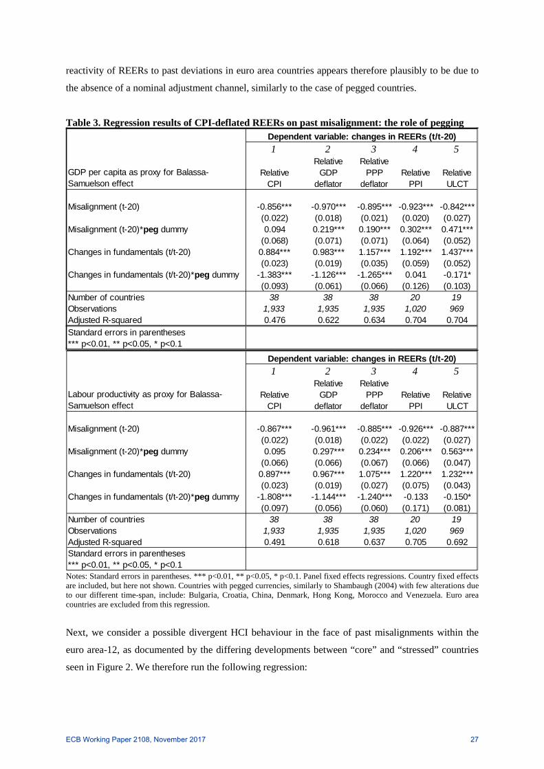
reactivity of REERs to past deviations in euro area countries appears therefore plausibly to be due to

the absence of a nominal adjustment channel, similarly to the case of pegged countries.

Table 3. Regression results of CPI-deflated REERs on past misalignment: the role of pegging

Notes: Standard errors in parentheses. *** p<0.01, ** p<0.05, * p<0.1. Panel fixed effects regressions. Country fixed effects are included, but here not shown. Countries with pegged currencies, similarly to Shambaugh (2004) with few alterations due to our different time-span, include: Bulgaria, Croatia, China, Denmark, Hong Kong, Morocco and Venezuela. Euro area countries are excluded from this regression.

Next, we consider a possible divergent HCI behaviour in the face of past misalignments within the

euro area-12, as documented by the differing developments between “core” and “stressed” countries

seen in Figure 2. We therefore run the following regression:

1 2 3 4 5

Relative CPI

Relative GDP

deflator

Relative PPP

deflatorRelative

PPIRelative ULCT

Misalignment (t-20) -0.856*** -0.970*** -0.895*** -0.923*** -0.842***(0.022) (0.018) (0.021) (0.020) (0.027)

Misalignment (t-20)*peg dummy 0.094 0.219*** 0.190*** 0.302*** 0.471***(0.068) (0.071) (0.071) (0.064) (0.052)

Changes in fundamentals (t/t-20) 0.884*** 0.983*** 1.157*** 1.192*** 1.437***(0.023) (0.019) (0.035) (0.059) (0.052)

Changes in fundamentals (t/t-20)*peg dummy -1.383*** -1.126*** -1.265*** 0.041 -0.171*(0.093) (0.061) (0.066) (0.126) (0.103)

Number of countries 38 38 38 20 19Observations 1,933 1,935 1,935 1,020 969Adjusted R-squared 0.476 0.622 0.634 0.704 0.704Standard errors in parentheses*** p<0.01, ** p<0.05, * p<0.1

Dependent variable: changes in REERs (t/t-20)

GDP per capita as proxy for Balassa-Samuelson effect

1 2 3 4 5

Relative CPI

Relative GDP

deflator

Relative PPP

deflatorRelative

PPIRelative ULCT

Misalignment (t-20) -0.867*** -0.961*** -0.885*** -0.926*** -0.887***(0.022) (0.018) (0.022) (0.022) (0.027)

Misalignment (t-20)*peg dummy 0.095 0.297*** 0.234*** 0.206*** 0.563***(0.066) (0.066) (0.067) (0.066) (0.047)

Changes in fundamentals (t/t-20) 0.897*** 0.967*** 1.075*** 1.220*** 1.232***(0.023) (0.019) (0.027) (0.075) (0.043)

Changes in fundamentals (t/t-20)*peg dummy -1.808*** -1.144*** -1.240*** -0.133 -0.150*(0.097) (0.056) (0.060) (0.171) (0.081)

Number of countries 38 38 38 20 19Observations 1,933 1,935 1,935 1,020 969Adjusted R-squared 0.491 0.618 0.637 0.705 0.692Standard errors in parentheses*** p<0.01, ** p<0.05, * p<0.1

Labour productivity as proxy for Balassa-Samuelson effect

Dependent variable: changes in REERs (t/t-20)


(10) ∆𝑟𝑟𝑒𝑒𝑒𝑒𝑟𝑟𝑡𝑡/(𝑡𝑡−20) = 𝛼𝛼𝑖𝑖 + 𝛽𝛽1 𝑚𝑚𝑟𝑟𝑟𝑟𝑡𝑡−20 + 𝛽𝛽2 𝑟𝑟𝑟𝑟𝑟𝑟𝑒𝑒𝑟𝑟𝑟𝑟𝑒𝑒𝑟𝑟 ∗ 𝑚𝑚𝑟𝑟𝑟𝑟𝑡𝑡−20 + 𝛾𝛾1 ∆𝑓𝑓𝑢𝑢𝑟𝑟𝑡𝑡/(𝑡𝑡−20) + 𝛾𝛾2 𝑟𝑟𝑟𝑟𝑟𝑟𝑒𝑒𝑟𝑟𝑟𝑟𝑒𝑒𝑟𝑟 ∗ ∆𝑓𝑓𝑢𝑢𝑟𝑟𝑡𝑡/(𝑡𝑡−20) +

𝜀𝜀 𝑡𝑡

According to CPI-deflated results reported in Table 4, also confirmed by the other deflators as shown

in Annex B, the sensitivity of HCIs to past misalignments in “stressed” countries was larger than that

of the other euro area countries, although this finding is entirely due to post-2009 developments.

Table 4. Regression results of CPI-deflated HCIs on past misalignments in “stressed” euro area countries

Notes: Standard errors in parentheses. *** p<0.01, ** p<0.05, * p<0.1. Panel fixed effects regressions. Country fixed effects are included, but here not reported. “Stressed” euro area countries include all 19 euro area countries except for Austria, Belgium, Finland, France, Germany, Luxembourg and the Netherlands.

4.2.2 Assessing the role of regulatory and institutional quality in the REER adjustment process

Finally, we consider the role of another variable in the REER correction process, namely that of

regulatory and institutional quality. The latter may affect REER adjustments via at least two channels.

The first relates to the political economy of sustained REER misalignments. Firms and economic

agents in general have different attitudes towards real exchange rates: exporters are likely to be

against overvalued currencies, whereas importers are penalised by undervalued currencies; similarly,

firms operating in tradable sectors are more prone to suffer from positive REER misalignments than

enterprises active in the non-tradable sector (documented on firm-level survey data by Broz, Freiden

and Weimouth, 2008). Rodrik (2008) argues that weak institutions exert “taxes” on both the tradable

and the non-tradable sectors, yet to a larger extent on the former, leading to a misallocation of the

economy’s resources, an under-sized tradable sector and sub-optimal growth. Under these

circumstances real undervaluation can promote economic growth. On the other hand, as discussed in

Christiansen et al. (2009), in countries with better institutions the political process may be less likely

to favour certain groups of interest with respect to others and are therefore less keen on tolerating

misaligned real exchange rates and more active in correcting existing disequilibria. In particular,

Nouira and Sekkat (2015) find a significant, negative relationship between democratic accountability

and real currency misalignments in a panel of emerging economies. Accountability indeed exposes

1999-2016Q3 <2009 ≥2009 1999-2016Q3 <2009 ≥2009Dependent variable: changes in CPI-based REERs (t/t-20) (1) (2) (3) (1) (2) (3)

Misalignment (t-20) -0.627*** -0.803*** -0.327*** -0.609*** -0.816*** -0.339***(0.025) (0.043) (0.043) (0.026) (0.044) (0.049)

Misalignment (t-20)*Stressed -0.332*** 0.036 -0.687*** -0.489*** 0.017 -0.807***(0.050) (0.065) (0.068) (0.056) (0.065) (0.090)

Changes in fundamentals (t/t-20) 0.179*** 0.104*** 0.113*** 0.204*** 0.044 0.116***(0.027) (0.033) (0.024) (0.034) (0.038) (0.032)

Changes in fundamentals (t/t-20)*Stressed 0.460*** 0.356*** 0.597*** 0.589*** 0.386*** 0.880***(0.042) (0.061) (0.055) (0.062) (0.072) (0.088)

Number of countries 12 12 12 12 12 12Observations 612 240 372 612 240 372Adjusted R-squared 0.819 0.775 0.614 0.794 0.777 0.517

GDP per capita Labour productivity


policymakers to the sanction of voters and therefore leads to more active corrections of currency

misalignments.

The second channel through which regulatory and institutional quality can affect the degree of

persistence of REER misalignments concerns the extent of structural rigidities in the economy.

Countries need to be flexible to allow relative prices to adjust to shocks (see, for example, Franks et

al., 2017). Prices and wages, and therefore REERs, can adjust more quickly in the absence of

structural rigidities. The latter may however be present due, amongst other factors, to strict product

and labour market regulation, an inefficient judicial system, a corrupt environment, which all distort

the efficient allocation of production factors across firms (on the presence of input misallocation in

the EU explained by these factors see Gamberoni et al. 2016; Gamberoni, Giordano and Lopez-

Garcia, 2016).

We therefore test the hypothesis of differences in the quality of regulation and institutions in affecting

the persistence of REER misalignments in our sample of countries.41 In particular, we augment

specification (6) with an interaction term between real misalignment and one of six indicators of

governance sourced from the World Bank.42 Three indicators refer to accountability, political stability

and government effectiveness, which capture the first channel and other three refer to regulatory

quality, rule of law and control of corruption, which take into account the second channel discussed.

An increase in any indicator implies an improvement in the quality of the institutional dimension

considered. Table B13 of Annex B provides summary statistics of these governance indicators for the

full sample and for three different country groupings over the whole period.

The new full specification is thus the following, where gov represents one of the six mentioned

governance indicators:

(11) ∆𝑟𝑟𝑒𝑒𝑒𝑒𝑟𝑟𝑡𝑡/(𝑡𝑡−20) = 𝛼𝛼𝑖𝑖 + 𝛽𝛽1 𝑚𝑚𝑟𝑟𝑟𝑟𝑡𝑡−20 + 𝛽𝛽2 𝑚𝑚𝑟𝑟𝑟𝑟𝑡𝑡−20 ∗ 𝑟𝑟𝑟𝑟𝑟𝑟𝑡𝑡−20 + 𝛽𝛽3 𝐸𝐸𝐸𝐸 ∗ 𝑚𝑚𝑟𝑟𝑟𝑟𝑡𝑡−20 + 𝛾𝛾1 ∆𝑓𝑓𝑢𝑢𝑟𝑟𝑡𝑡/(𝑡𝑡−20) + 𝛾𝛾2 𝐸𝐸𝐸𝐸 ∗

∆𝑓𝑓𝑢𝑢𝑟𝑟𝑡𝑡/(𝑡𝑡−20) + 𝜀𝜀 𝑡𝑡

Regression results in Table 5, based on CPI deflators but confirmed by all deflators,43 show that on

average in all countries the reactivity of REERs to past deviations from equilibrium values increases

the better a country scores in terms of all dimensions of regulatory and institutional quality, with the

exception of political stability, suggesting that both channels are at play in our sample of countries.

Moreover, the non-significance of 𝛽𝛽3 across all specifications implies that the role of institutions in

41 One could argue that institutional quality is a determinant of real exchange rates and, therefore, should be included as anexplanatory variable in the BEER model. On the one hand, countries with better governance may attract more foreign capitalinflows, as a result of low expropriation risks, and thus lead to an appreciated currency. On the other hand, as discussed inChristiansen et al. (2009), better institutions may generate an environment more conducive to saving, which leads to lessdemand for goods and a more depreciated real exchange. To our knowledge no existing BEER model includes institutionalvariables, also because the link to real exchange rates is not theoretically grounded. Moreover, institutional variables mainlyexhibit a cross-sectional variation and are therefore captured indirectly by the country fixed effects in equation (4). For thesereasons, we only consider the possible impact of institutions on the REER adjustment process, via the two channelsdiscussed in the main text.42 The indicators are available at the following website: http://info.worldbank.org/governance/wgi.43 Results based on the other deflators are available upon request.


http://info.worldbank.org/governance/wgi

the adjustment process is as important for euro area countries as it is for non-euro area advanced and

emerging economies.44

To sum up, misalignments are found to have been more persistent in the euro area than in countries

with different nominal exchange rate regimes, at least until 2009. Indeed, in a monetary union,

abstracting from varying trade patterns, changes in real exchange rates can take place only through

inflation differentials, since nominal exchange rates are fixed by definition. The larger persistence in

real misalignments in the euro area may thus be linked to the adoption of the single currency. The

lower persistence of misalignments in the recent recessionary phase, driven mainly by the higher

sensitivity of HCIs to past disequilibria in stressed countries, is plausibly linked to the structural

reforms enacted as a result of the global financial crisis in these countries, which removed existing

real rigidities, and to a lower “tolerance” of REER misalignments, in turn speeding up the adjustment

process. Indeed, according to standard OECD indicators on both product and labour market

legislation, where the extent of deregulation in the years prior to the crisis were comparable in both

euro and non-euro area advanced economies, in the more recent period since 2009 reform action was

relatively bolder in euro area countries, and in particular in the “stressed” euro area countries.45

44 In a robustness check we also investigated whether the level of development of an economy may affect the persistence of misalignments. We therefore interacted the misalignment variable with relative GDP per capita. Results vary across the differently deflated REERs but generally point to insignificant interaction terms. This implies that it is indeed the regulation and institution channels that affect the reactivity of REERs to past misalignments and not more generally the level of development of an economy. 45 On this last point see also Franks et al. (2017).


Table 5. Regression results of CPI-deflated REERs on past misalignment: the role of institutions

Notes: Panel fixed effects regressions. Country fixed effects are included, but here not reported. Standard errors in parentheses. *** p<0.01, ** p<0.05, * p<0.1.

GDP per capita

Labour productivity

GDP per capita

Labour productivity

1999-2015 1999-2015 1999-2015 1999-2015Dependent variable: changes in CPI-based REERs (t/t-20) (1) (2)

Dependent variable: changes in CPI-based REERs (t/t-20) (1) (2)

Misalignment (t-20) -0.727*** -0.743*** Misalignment (t-20) -0.749*** -0.751***(0.023) (0.023) (0.020) (0.020)

Misalignment (t-20)*Regulatory quality (t-20) -0.082*** -0.041* Misalignment (t-20)*Rule of law (t-20) -0.064*** -0.042**(0.023) (0.024) (0.019) (0.019)

Misalignment (t-20)*EA dummy 0.292*** 0.259** Misalignment (t-20)*EA dummy 0.181** 0.144*(0.108) (0.116) (0.073) (0.077)

Misalignment (t-20)*Regulatory quality (t-20)*EA dummy -0.128 -0.137

Misalignment (t-20)*Rule of law (t-20)*EA dummy -0.038 -0.038

(0.096) (0.101) (0.070) (0.073)Changes in fundamentals (t/t-20) 0.848*** 0.806*** Changes in fundamentals (t/t-20) 0.831*** 0.804***

(0.025) (0.026) (0.023) (0.023)Changes in fundamentals (t/t-20)*EA dummy -0.388*** -0.313*** Changes in fundamentals (t/t-20)*EA dummy -0.349*** -0.285***

(0.049) (0.056) (0.046) (0.052)Number of countries 57 57 Number of countries 57 57Observations 2,902 2,902 Observations 2,902 2,902Adjusted R-squared 0.441 0.421 Adjusted R-squared 0.440 0.421

GDP per capita

Labour productivity

GDP per capita

Labour productivity




Misalignment (t-20)*Control of corruption (t-20) -0.048*** -0.022 Misalignment (t-20)*Accountability (t-20) -0.070*** -0.059**(0.018) (0.018) (0.026) (0.027)

Misalignment (t-20)*EA dummy 0.131** 0.106 Misalignment (t-20)*EA dummy 0.338** 0.261(0.064) (0.067) (0.170) (0.179)

Misalignment (t-20)*Control of corruption (t-20)*EA dummy 0.002 -0.008

Misalignment (t-20)*Accountability (t-20)*EA dummy -0.170 -0.127



(0.046) (0.051) (0.046) (0.052)Constant 0.001 0.001 Constant 0.001 0.001


GDP per capita

Labour productivity

GDP per capita

Labour productivity




Misalignment (t-20)*Government effectiveness (t-20) -0.051** -0.033 Misalignment (t-20)*Political stability (t-20) -0.025 -0.025(0.022) (0.022) (0.023) (0.023)

Misalignment (t-20)*EA dummy 0.193** 0.151 Misalignment (t-20)*EA dummy 0.182 0.068(0.094) (0.098) (0.129) (0.132)

Misalignment (t-20)*Government effectiveness (t-20)*EA dummy -0.051 -0.043

Misalignment (t-20)*Political stability (t-20)*EA dummy -0.037 0.049



(0.046) (0.051) (0.042) (0.047)Constant 0.001 0.001 Constant 0.001 0.001


Panel A. Regulatory quality

Panel C. Control of corruption

Panel E. Government effectiveness Panel F. Political stability

Panel B. Rule of law

Panel D. Accountability


5 Conclusions

This paper draws upon a Behavioural Equilibrium Exchange Rate (BEER) model in order to analyse

the magnitude and persistence of real currency misalignments within the euro area to assess any

differences with respect to other countries that have adopted different nominal exchange rate

arrangements. It therefore contributes to the literature aimed at investigating whether countries in a

currency union or with fixed exchange rates have worse outcomes for REERs than countries with

flexible exchange rates.

In the construction and estimation of the BEER model, particular care is given to: a) the selection of

the economic fundamentals to be included in the specification and to the estimation of the so-called

Balassa-Samuelson effect, i.e. the impact of relative productivity levels on real effective exchange

rates; b) the dataset employed: the BEER model is estimated for a larger sample of countries and at a

higher frequency than what is usually done in the literature; moreover, given that recent studies

suggest that no optimal deflator exists for REERs, we estimate the model using five alternatively

deflated REERs; c) the panel cointegration estimation method, which, amongst various desirable

properties, accounts for cross-section dependence, resulting from the fact that countries may be

affected by common, global shocks.

Our BEER estimation results are consistent with economic theory. We find a significant and positive

relationship between real exchange rates and either GDP per capita or labour productivity, i.e.

significant evidence of the Balassa-Samuelson effect, in the broad sample of countries at least.

Moreover, real appreciation is found to be associated with higher trade restrictions, proxied by lower

trade openness, higher terms of trade, higher government expenditure and higher short-term real

interest rates. Using these estimated relationships, we construct measures of REER misalignments in

order to tackle our research question.

Our findings are the following. Since 1999 misalignments of HCIs (the equivalent of REERs for euro

area countries) have been found to be significantly smaller in euro area economies in comparison with

the other countries in our sample, and even more so in the recent recessionary phase. Based on these

results, one cannot easily make the case that the adoption of the euro amplified misalignments, but

rather the single currency seems to have curbed these misalignments, plausibly by removing a

significant source of volatility stemming from financial market shocks. Within the euro area

“stressed” countries recorded larger misalignments than “core” countries, yet only until 2009, after

which a sharp downward correction was enacted in the former set of economies.

Although smaller to those observed in non-euro area countries, HCI misalignments in the euro area

are however found to be more persistent. Indeed, there is evidence of a significant REER adjustment

process also within the euro area, yet the reactivity of HCIS in euro area countries is on average more

contained than that of the other economies in the sample. After 2009, however, the sensitivity of euro

area HCIs to past misalignments increased significantly relative to the previous period.


On the back of the evidence in this paper, one could make the case that the policies enacted in order to

adopt the euro prior to 1999 led to the reaping of the “low-hanging fruits” of a currency union,

signalled by small real exchange rate misalignments as of 1999. Yet, the remaining disequilibria

turned out to be more persistent relative to those of countries outside the euro area, owing to the

absence of a nominal adjustment channel and to that fact that the pace of structural reforms after 1999

within the euro area was no faster than that observed in other economies, at least according to

standard OECD regulatory indicators. However, as of 2009 the difference in reactivity of REERs to

past misalignments between euro vs. non-euro area countries has significantly narrowed, if not

evaporated completely according to the different REER deflator considered, mainly due to faster

adjustment in the “stressed” euro area-12 countries. This result could be due to cyclical factors, linked

to the severe recession the area euro experienced, and thus could be expected to be reversible. But it is

also due to structural factors, tied to enhanced reform action implemented as a result of the crisis in

the euro area (relative to other non-euro area advanced economies) and especially in the “stressed”

euro area countries, leading to a lower persistence of real effective exchange rate misalignments in the

euro area in recent years relative to the pre-2009 years. We indeed find significant empirical evidence

that improving various dimensions of domestic regulation and institutions favours the REER

correction process, even for euro area countries, since it removes structural rigidities and thus can

partly compensate for the loss of the nominal adjustment channel that the adoption of a single

currency implies.


Annex A. The Balassa-Samuelson effect

The intuition behind the Balassa-Samuelson effect may be formally derived assuming two two-sector

economies, Home and Foreign.46 If we consider in a static framework a two-sector small economy,

Home, that produces both tradable and non-tradable goods using only homogeneous labour as an

input, the general price index P may be considered as a geometric average of the Home tradable and

non-tradable goods.

(A1) 𝑃𝑃 ≡ 𝑃𝑃𝑇𝑇𝜃𝜃𝑃𝑃𝑁𝑁𝑇𝑇(1−𝜃𝜃)

where 𝑃𝑃𝑇𝑇 and 𝑃𝑃𝑁𝑁𝑇𝑇 are the prices of tradables and non tradables, respectively, and 0 < 𝜃𝜃 < 1. In the

long run labour is perfectly mobile between sectors so that long-run real wages in the two sectors are

equal: 𝑊𝑊𝑁𝑁𝑃𝑃

= 𝑊𝑊𝑁𝑁𝑁𝑁𝑃𝑃

= 𝑊𝑊𝑃𝑃

, where 𝑤𝑤𝑇𝑇 and 𝑤𝑤𝑁𝑁𝑇𝑇 are the wages in the tradable and non-tradable sector,

respectively; the nominal wages are also equalised between sectors in the long run. Under perfect

competition, the nominal wages are also equal to the marginal revenue product of labour: 𝑤𝑤𝑇𝑇 =

𝑃𝑃𝑇𝑇𝐸𝐸𝑇𝑇 = 𝑊𝑊 and 𝑤𝑤𝑁𝑁𝑇𝑇 = 𝑃𝑃𝑁𝑁𝑇𝑇𝐸𝐸𝑁𝑁𝑇𝑇 = 𝑊𝑊, where 𝐸𝐸𝑇𝑇 and 𝐸𝐸𝑁𝑁𝑇𝑇 is the marginal product of labour in,

respectively, the tradable and non-tradable sectors. Therefore:

(A2) 𝑃𝑃𝑁𝑁𝑁𝑁𝑃𝑃𝑁𝑁

= 𝐴𝐴𝑁𝑁𝐴𝐴𝑁𝑁𝑁𝑁

Or, in other terms, relative prices of non-traded and traded goods in a country are inversely related to

the relative productivity in the two sectors. The relative price of non-tradable goods is thus entirely

determined by technology and is independent of demand conditions. Taking into account the identity

(A1):

(A3) 𝑃𝑃 = 𝑃𝑃𝑇𝑇( 𝐴𝐴𝑁𝑁𝐴𝐴𝑁𝑁𝑁𝑁

)(1−𝜃𝜃)

In other terms, relatively higher productivity growth in the tradable sector leads to an overall price rise

in the long-run.

Assuming the law of one price holds for traded goods in the long run, this implies, as seen already in

equation (3) in the main text:

(A4) 𝑃𝑃𝑇𝑇 ∗ = 𝑒𝑒𝑃𝑃𝑇𝑇

where * indicates a foreign country (Foreign) and e is the exchange rate (i.e the Foreign price in

Home currency). Assuming Foreign has the same economic structure as Home, the following equation

also holds:

(A5) 𝑃𝑃∗ = 𝑃𝑃𝑇𝑇∗( 𝐴𝐴𝑁𝑁∗

𝐴𝐴𝑁𝑁𝑁𝑁∗)(1−𝜃𝜃∗)

Equations (A3), (A4) and (A5) lead to the following equation for the long-run real exchange rate Q:

(A6) Q≡ 𝑒𝑒𝑃𝑃𝑃𝑃∗

= ( 𝐴𝐴𝑁𝑁𝐴𝐴𝑁𝑁𝑁𝑁

)(1−𝜃𝜃)/( 𝐴𝐴𝑁𝑁∗

𝐴𝐴𝑁𝑁𝑁𝑁∗)(1−𝜃𝜃∗)

if the consumption basket of tradables and non-tradables is similar in both countries, i.e. 𝜃𝜃 = 𝜃𝜃∗, then

the long-run real exchange rate is determined by the productivity differential between the tradable and

46 The simplified derivation presented here is taken from Obstfeld and Rogoff (1996) and Lothian and Taylor (2008).


non-tradable sectors in Home relative to that in Foreign.47 If the productivity differential is the same

in the two countries, then E = 1 (i.e. the absolute purchasing power parity level).48

As shown in Lothian and Taylor (2008), supposing that productivity in the non-tradable sector is

constant in both Home and Foreign, and taking logarithms of equation (A6), we obtain:

(A7) 𝑞𝑞 = 𝛾𝛾0 + 𝛾𝛾1 𝑎𝑎𝑇𝑇 − 𝛾𝛾2 𝑎𝑎 𝑇𝑇∗

where lower cases denote logarithms, γ0 = −(1 − θ)aN + (1 − θ∗)a N∗ , 𝛾𝛾1 = (1 − θ) > 0 and 𝛾𝛾2 =

(1 − θ∗) < 0. In general, equation (A7) suggests that, in a static setting, prices are higher in higher-

(tradable) productivity countries relative to those in lower-(tradable) productivity countries; in a

dynamic context, prices in faster (tradable) productivity-growing countries will rise relative to prices

in slower (tradable) productivity-growing countries. If productivity in the non-tradable sector is

constant across countries, for example because it is considered close to zero in many countries, γ0

becomes a constant,49 the exchange rate is proportional only to the tradable sector’s productivity, as is

total productivity.

47 As Froot and Rogoff (1994) explain, if two countries have different weights of tradables in their consumption baskets(i. e.θ ≠θ∗in equation A6), but identical technologies (A∗NT = ANT and A∗T = AT ), this is sufficient to yield a trend in thereal exchange rate. Ultimately, for the real exchange rate to converge in the long run, one must have convergence in tastes,as well as technology.48 Balassa’s (1964) model explains deviations from the absolute purchasing power parity. As discussed in Bergin, Glick andTaylor (2006), the Balassa-Samuelson effect is not guaranteed to exist, as it assumes that innovation is mainly concentratedin the tradable sector and thus that the growth path of an economy is biased towards this sector. If the sources of growth areevenly spread out between the tradable and non-tradable sectors (i.e. balanced growth hypothesis), the effect does notappear, unless non-traded goods are relatively more labour-intensive than traded goods, as Froot and Rogoff (1994) showusing an extension of the simplified Balassa-Samuelson model shown here to a two-factor production model with perfectlymobile capital. Moreover, if technological changes were biased toward non-tradable goods (i.e. biased growth), then a pricelevel could actually fall if countries get richer, leading to the opposite of the Balassa-Samuelson effect (see, for example,Devereux, 1999 for evidence of a counter Balassa-Samuelson effect due to high productivity growth in distribution servicesas a result of productivity gains in manufacturing). Ultimately, the presence of the Balassa-Samuelson effect is an empiricalissue. For it to emerge over time, either the biasedness of productivity growth towards the tradable sector has to increase orthe share of non-traded goods should increase over time, both plausible facts. Finally, see Hassan (2016) for a discussion of apossible non-monotonicity of the Balassa-Samuelson effect. We refer to Section 2 for the empirical evidence of the Balassa-Samuelson effect in our sample of countries.49 This assumption is strong, yet there is evidence for many countries over long time spans that productivity growth inservice sectors, a proxy of the non-tradable sector, is significantly slower to that of sectors open to trade and often close tozero (see e.g., Timmer, Inklar and O’Mahoney, 2010; Broadberry, Giordano and Zollino, 2013; Giordano, Toniolo andZollino, 2017).


Annex B. Additional tables and figures

Table B1. An overview of variables included in a selection of BEER models

Notes: A=annual; Q=quarterly. The explanatory variables reported are those included in the baseline specifications of the selected studies. When the + or - sign is omitted the estimated relationship is not statistically significant.

References Countries Time-span Frequency Explanatory variables Deflator Estimation methodologyComunale (2017) 27 (EU

countries)1994-2012 A Foreign net capital inflows (+); terms of

trade(+); GDP per capita(+)CPI GM-FMOLS

Hajek (2016) 12 (EA countries)

1980-2014 A GDP per capita(+); trade balance (-); terms of trade (+)

CPI DOLS

Gnimassoun and Mignon (2015)

22 (industrialized countries )

1980-2011 A GDP per capita (+): net foreign assets in percentage of GDP (+)

CPI DOLS

Adler and Grisse (2014)

a) 21 b) 23 (advanced economies)

a) 1980-2011b) 1995-2011

A a) GDP per capita(+); government consumption(+); labour productivity(-); netforeign assets(+); terms of trade(+)b) GDP per capita; government consumption(+); labour productivity; netforeign assets; terms of trade(+)

CPI DOLS

Fischer and Hossfeld (2014)

57(advanced and emerging economies)

1980-2011 A Labour productivity(+) PPP a) Panel OLSb) Pooled OLSc) Panel DOLS

Mancini-Griffolo, Meyer, Natal and Zanetti (2014)

18 (advanced economies)

1973-2011 A Net foreign assets(+); output per capita(+); terms of trade(+); government consumption(+); sectorial labour productivity

CPI; PPI DOLS

Coudert, Couhart and Mignon (2013)

11 (EA countries)

1980-2010 A GDP per capita (+): net foreign assets in percentage of GDP (+)

CPI DOLS

Bussière, Ca’ Zorzi, Chudík, Dieppe (2010)

a) 44 b) 14 (advancedand emerging economies)

1980-2007 a) Ab) Q

Commodity terms of trade(+); fiscal policy(+); civil liberties(-); openness(-); net foreign assets; investment; government spending; trade restriction index; GDP per capita (+); commodity prices

PPP Single-country estimations:Autoregressive distributed lag approach (ARDL).Pure cross section and panel estimations: common correlated effects mean group estimators(CCEMG); common correlated effects pooled (CCEP)

Hossfeld (2010) 17(US and its 16 major trading partners)

1986-2006 Q Net foreign assets to GDP(-); trade balance to GDP; terms of trade(+); government consumption; openness

CPI Single country estimations: a) DOLS; b) FMOLSPanel estimations:a) Group-mean DOLS;b) FMOLS.

Bénassy-Queré, Béreau and Mignon (2009)

15 GDP per capita (+): net foreign assets in percentage of GDP (+); real interest rate differentials (+); terms of trade (+)

CPI DOLS

Ricci, Milesi-Ferretti and Lee (2008)

48(advanced and emerging economies)

1980-2004 A Trade restriction index(+); price controls(-); commodity terms of trade(+); net foreign assets to trade(+);government consumption to GDP(+); labour productivity tradables(+); labour productivity nontradables(-)

CPI a) DOLSb) FMOLS

Lane and Milesi-Ferretti (2004)

64 (industrial and middle-income developing countries)

1975-1996 A Net foreign assets (+); GDP per capita (+); terms of trade (+)

CPI; WPI Cross-section and panel estimations: DOLS

Maeso Fernández, Osbat and Schnatz (2004)

25(OECD countries)

1975-2002 A GDP per capita(+); government spending to GDP(+); openness(-)

PPP a) Error correction mean-groupestimator (MGE /PMGE)b) FMOLS (weighted / unweighted)c) DOLS (weighted / unweighted)

Maeso Fernández, Osbat and Schnatz (2001)

23(advanced economies)

1975-1998 Q Labour productivity (+); accumulated current account to GDP; real price of oil(+); long-term interest rate differential(-)

CPI VECM

Clark and MacDonald (1998)

7(G-7 countries)

1960-1996 A Terms of trade(+); CPI/PPI ratio(+); net foreign assets as ratio of GDP(+); relative stock of government debt(+); real interest rate(-)

CPI Johansen cointegration method


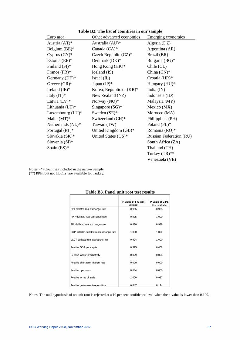
Table B2. The list of countries in our sample Euro area Other advanced economies Emerging economies Austria (AT)* Australia (AU)* Algeria (DZ) Belgium (BE)* Canada (CA)* Argentina (AR) Cyprus (CY)* Czech Republic (CZ)* Brazil (BR) Estonia (EE)* Denmark (DK)* Bulgaria (BG)* Finland (FI)* Hong Kong (HK)* Chile (CL) France (FR)* Iceland (IS) China (CN)* Germany (DE)* Israel (IL) Croatia (HR)* Greece (GR)* Japan (JP)* Hungary (HU)* Ireland (IE)* Korea, Republic of (KR)* India (IN) Italy (IT)* New Zealand (NZ) Indonesia (ID) Latvia (LV)* Norway (NO)* Malaysia (MY) Lithuania (LT)* Singapore (SG)* Mexico (MX) Luxembourg (LU)* Sweden (SE)* Morocco (MA) Malta (MT)* Switzerland (CH)* Philippines (PH) Netherlands (NL)* Taiwan (TW) Poland (PL)* Portugal (PT)* United Kingdom (GB)* Romania (RO)* Slovakia (SK)* United States (US)* Russian Federation (RU) Slovenia (SI)* South Africa (ZA) Spain (ES)* Thailand (TH)

Turkey (TR)** Venezuela (VE)

Notes: (*) Countries included in the narrow sample. (**) PPIs, but not ULCTs, are available for Turkey.

Table B3. Panel unit root test results

Notes: The null hypothesis of no unit root is rejected at a 10 per cent confidence level when the p-value is lower than 0.100.

P-value of IPS teststatistic

P-value of CIPS test statistic

CPI-deflated real exchange rate 0.995 0.998

PPP-deflated real exchange rate 0.995 1.000

PPI-deflated real exchange rate 0.830 0.999

GDP deflator-deflated real exchange rate 1.000 1.000

ULCT-deflated real exchange rate 0.994 1.000

Relative GDP per capita 0.395 0.468

Relative labour productivity 0.829 0.008

Relative short-term interest rate 0.000 0.000

Relative openness 0.084 0.000

Relative terms of trade 1.000 0.987

Relative government expenditure 0.847 0.194


Table B4. Panel cointegration test results

Notes: The null hypothesis of no cointegration is rejected at a 10 per cent confidence level when the test statistics are lower than -1.29.

Pedroni (1999) group-mean rho

test statistic

Pedroni (1999) group-mean t test

statistic

Pedroni (1999) group-mean adf

test statistic

Productivity measure Additional variables

CPI-deflated real exchange rate Relative GDP per capitaRelative trade, interest rate

and government expenditure variables

2.890 -0.033 -2.118

PPP-deflated real exchange rate Relative GDP per capitaRelative trade, interest rate


2.802 -0.086 -2.296

PPI-deflated real exchange rate Relative GDP per capitaRelative trade, interest rate


2.170 -0.942 -2.411

Relative trade, interest rate and government expenditure

variables

GDP deflator-deflated real exchange rate Relative GDP per capitaRelative trade, interest rate


2.610 -0.618 -1.616


variables

ULCT-deflated real exchange rate Relative GDP per capitaRelative trade, interest rate


0.677 -2.703 -3.680


variables

CPI-deflated real exchange rate Relative labour productivityRelative trade, interest rate


2.873 -0.182 -2.773


variables

PPP-deflated real exchange rate Relative labour productivityRelative trade, interest rate


2.577 -0.558 -2.200


variables

PPI-deflated real exchange rate Relative labour productivityRelative trade, interest rate


1.614 -1.873 -3.524


variables

GDP deflator-deflated real exchange rate Relative labour productivityRelative trade, interest rate


2.759 -0.588 -1.993


variables

ULCT-deflated real exchange rate Relative labour productivityRelative trade, interest rate


1.226 -2.004 -3.229

Dependent variable Covariates


Table B5. BEER estimation results, 1999Q1-2008Q4


1 2 3 4 5

Relative CPI

Relative GDP

deflator

Relative PPP

deflatorRelative

PPIRelative ULCT

A.Relative GDP per capita 0.4756** 0.3043 0.3560* 0.1606 0.3126

(0.2149) (0.2121) (0.1996) (0.1964) (0.3282)Relative openness -0.2725*** -0.2677*** -0.2325*** -0.1373** -0.2475***

(0.0654) (0.0609) (0.0635) (0.0671) (0.0833)Relative terms of trade 0.1106 0.2754*** 0.3050*** 0.5302*** 0.2277

(0.0847) (0.1031) (0.1083) (0.1912) (0.2113)Relative government expenditure 0.3911 0.0128 0.5134* 0.0245 1.6845***

(0.2966) (0.2513) (0.2662) (0.2814) (0.3135)Relative short-term interest rates 0.0008 0.0020*** 0.0024*** -0.0001 -0.0004

(0.0008) (0.0007) (0.0007) (0.0008) (0.0010)

Number of countries 57 57 57 39 38Number of observations 2,280 2,280 2,280 1,560 1,520B.Relative labour productivity 0.1554 0.0822 0.1226 -0.3035* -0.3597*

(0.1425) (0.1679) (0.1526) (0.1662) (0.1850)Relative openness -0.2708*** -0.2874*** -0.2622*** -0.1016 -0.2028***

(0.0825) (0.0697) (0.0740) (0.0786) (0.0785)Relative terms of trade 0.2433** 0.3380*** 0.4216*** 0.3391* -0.0012

(0.1152) (0.1178) (0.1379) (0.2023) (0.1683)Relative government expenditure 0.3123 0.0967 0.4095 0.0814 1.5409***

(0.3049) (0.3187) (0.3026) (0.2436) (0.2476)Relative short-term interest rates 0.0009 0.0018** 0.0021*** -0.0000 -0.0010

(0.0007) (0.0008) (0.0008) (0.0007) (0.0009)


Dependent variable


Table B6. Narrow-sample CPI, GDP and PPP deflator estimation results


1 2 3

Relative CPI

Relative GDP

deflator

Relative PPP

deflatorA.Relative GDP per capita 0.0151 0.2602** 0.2800**

(0.1427) (0.1266) (0.1359)Relative openness -0.2864*** -0.2848*** -0.2568***

(0.0606) (0.0642) (0.0600)Relative terms of trade 0.1689 0.3783*** 0.4960***

(0.1177) (0.1052) (0.1337)Relative government expenditure 0.1865 0.1010 0.3509

(0.2112) (0.2320) (0.2429)Relative short-term interest rates 0.0021* 0.0029** 0.0035***

(0.0012) (0.0012) (0.0012)

Number of countries 38 38 38Number of observations 2,698 2,698 2,698B.Relative labour productivity 0.0459 0.0531 0.0589

(0.1360) (0.1116) (0.1240)Relative openness -0.2534*** -0.3019*** -0.2671***

(0.0626) (0.0698) (0.0667)Relative terms of trade 0.2656** 0.4586*** 0.5677***

(0.1042) (0.1127) (0.1189)Relative government expenditure -0.0762 -0.3634 -0.0662

(0.2417) (0.3283) (0.3057)Relative short-term interest rates 0.0022** 0.0015 0.0026*

(0.0011) (0.0014) (0.0013)

Number of countries 38 38 38Number of observations 2,698 2,698 2,698

Dependent variable


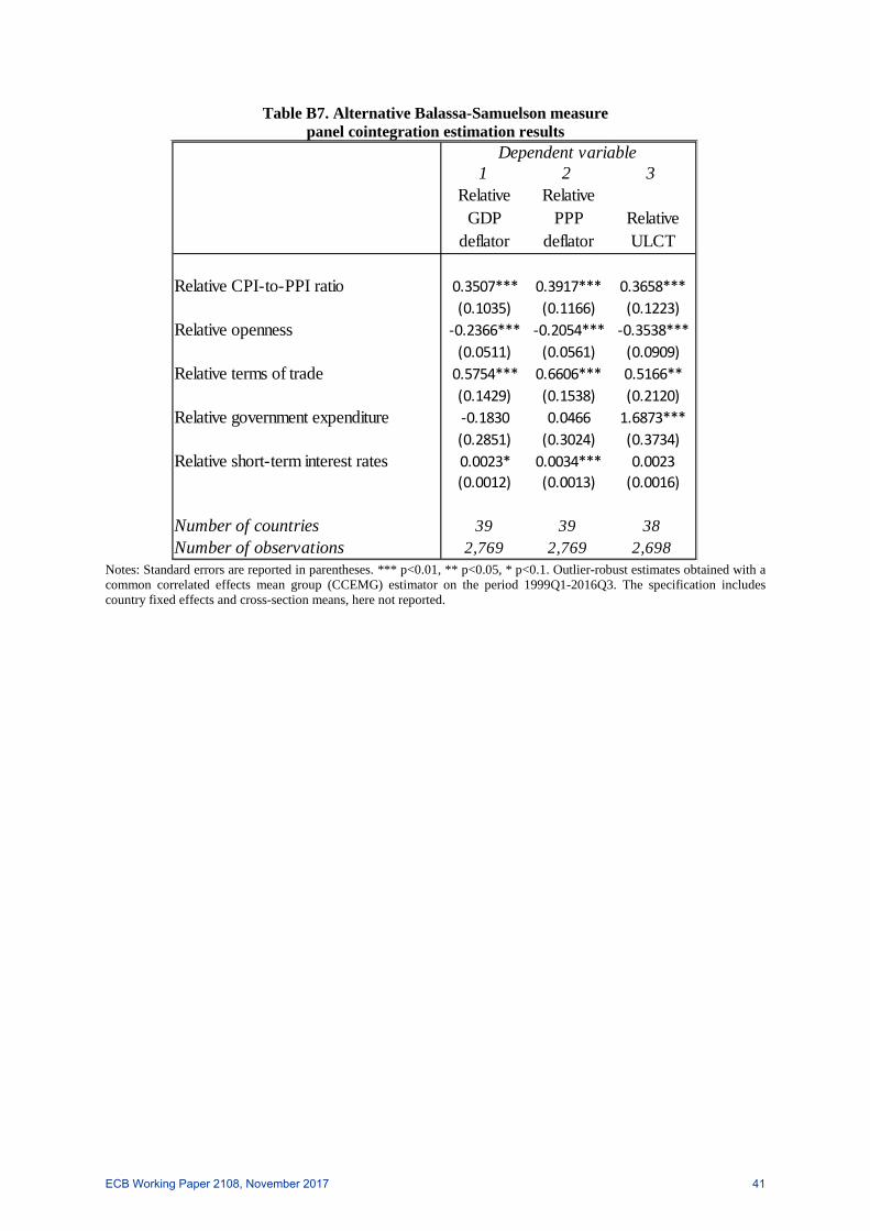
Table B7. Alternative Balassa-Samuelson measure panel cointegration estimation results


1 2 3Relative

GDP deflator

Relative PPP

deflatorRelative ULCT

Relative CPI-to-PPI ratio 0.3507*** 0.3917*** 0.3658***(0.1035) (0.1166) (0.1223)

Relative openness -0.2366*** -0.2054*** -0.3538***(0.0511) (0.0561) (0.0909)

Relative terms of trade 0.5754*** 0.6606*** 0.5166**(0.1429) (0.1538) (0.2120)

Relative government expenditure -0.1830 0.0466 1.6873***(0.2851) (0.3024) (0.3734)

Relative short-term interest rates 0.0023* 0.0034*** 0.0023(0.0012) (0.0013) (0.0016)

Number of countries 39 39 38Number of observations 2,769 2,769 2,698

Dependent variable


Table B8. Panel cointegration estimation results with additional explanatory variables


1 2 3 4 5Relative

CPIRelative

CPIRelative

CPIRelative

CPIRelative

CPIA.Relative GDP per capita 0.6373 0.2057 0.2128 0.0810 0.3396**


(0.0699) (0.0824) (0.0864) (0.0873) (0.0801)Relative terms of trade 0.1278* 0.1975** 0.2337** 0.3030** 0.1214

(0.0760) (0.0767) (0.1033) (0.1191) (0.0876)Relative government expenditure 0.1359 0.3307 0.2934 0.0093 0.4994**

(0.1888) (0.2302) (0.2183) (0.1770) (0.2185)Relative short-term interest rates -0.0007 -0.0001 -0.0002 0.0004 0.0004

(0.0006) (0.0007) (0.0007) (0.0008) (0.0009)Squared relative GDP per capita -0.5178

(1.0573)Relative participation rate -0.4823

(0.4205)Relative total population dependency rate 0.5291

(1.5303)Relative aging structure 1.3362

(1.6491)Relative investment rate -0.0032

(0.1223)Number of countries 57 57 51 51 57Number of observations 4,034 4,016 3,610 3,610 4,034B.Relative labour productivity 0.1002 0.1438 0.2005 0.2384 0.2605**


(0.0672) (0.0816) (0.0884) (0.0786) (0.0776)Relative terms of trade 0.1854* 0.1840** 0.2197** 0.2221** 0.1488*

(0.1064) (0.0787) (0.0871) (0.1040) (0.0847)Relative government expenditure -0.1605 0.1429 0.0891 0.0047 0.0776

(0.2843) (0.1979) (0.2175) (0.2849) (0.2749)Relative short-term interest rates 0.0007 -0.0000 0.0002 0.0005 0.0014

(0.0008) (0.0007) (0.0007) (0.0009) (0.0011)Squared relative labour productivity -0.6888

(0.7906)Relative participation rate 0.2611

(0.4629)Relative total population dependency rate 1.2944

(1.5121)Relative aging structure 1.0804

(1.7088)Relative investment rate -0.1083

(0.1397)Number of countries 57 57 51 51 57Number of observations 4,016 4,016 3,592 3,592 4,016

Dependent variable


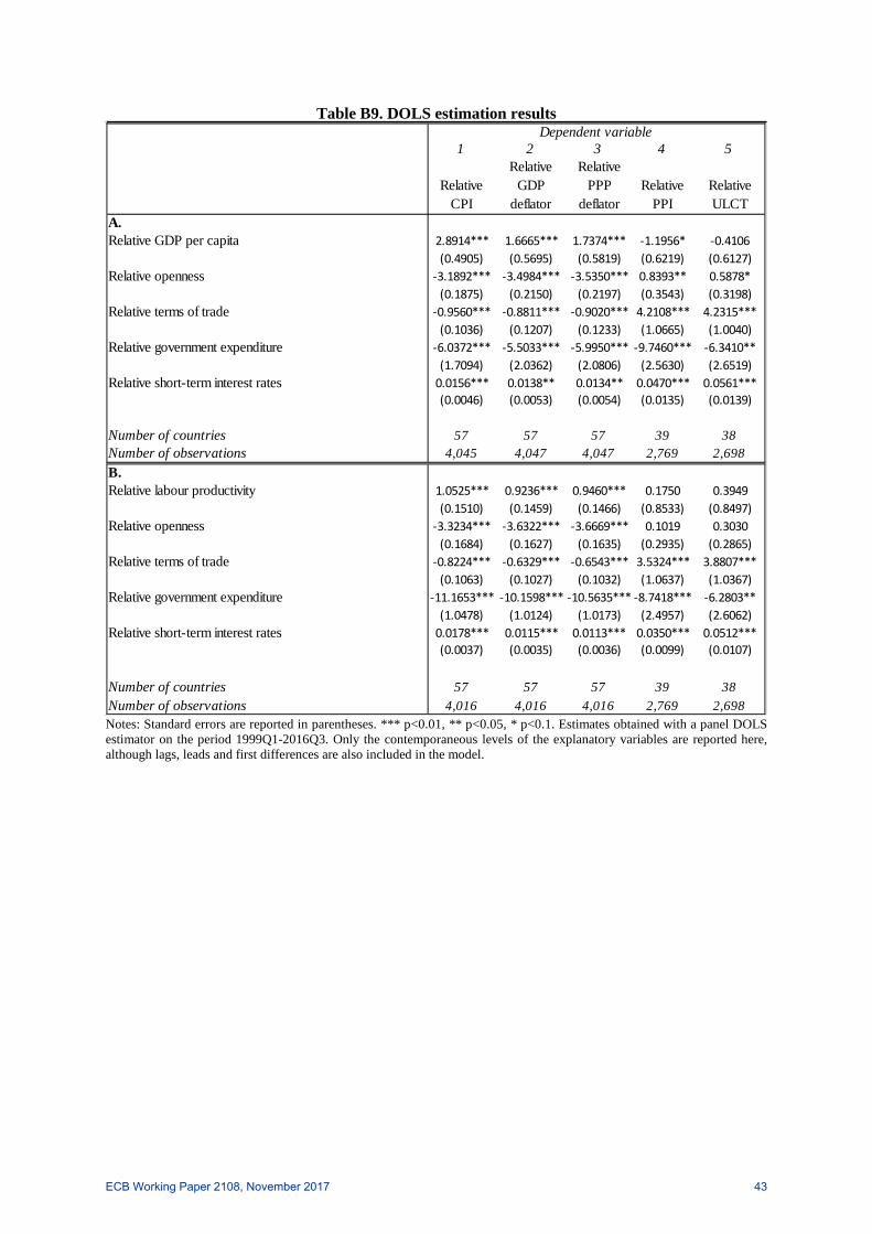
Table B9. DOLS estimation results

Notes: Standard errors are reported in parentheses. *** p<0.01, ** p<0.05, * p<0.1. Estimates obtained with a panel DOLS estimator on the period 1999Q1-2016Q3. Only the contemporaneous levels of the explanatory variables are reported here, although lags, leads and first differences are also included in the model.

1 2 3 4 5

Relative CPI

Relative GDP

deflator

Relative PPP

deflatorRelative

PPIRelative ULCT

A.Relative GDP per capita 2.8914*** 1.6665*** 1.7374*** -1.1956* -0.4106

(0.4905) (0.5695) (0.5819) (0.6219) (0.6127)Relative openness -3.1892*** -3.4984*** -3.5350*** 0.8393** 0.5878*

(0.1875) (0.2150) (0.2197) (0.3543) (0.3198)Relative terms of trade -0.9560*** -0.8811*** -0.9020*** 4.2108*** 4.2315***

(0.1036) (0.1207) (0.1233) (1.0665) (1.0040)Relative government expenditure -6.0372*** -5.5033*** -5.9950*** -9.7460*** -6.3410**

(1.7094) (2.0362) (2.0806) (2.5630) (2.6519)Relative short-term interest rates 0.0156*** 0.0138** 0.0134** 0.0470*** 0.0561***

(0.0046) (0.0053) (0.0054) (0.0135) (0.0139)

Number of countries 57 57 57 39 38Number of observations 4,045 4,047 4,047 2,769 2,698B.Relative labour productivity 1.0525*** 0.9236*** 0.9460*** 0.1750 0.3949

(0.1510) (0.1459) (0.1466) (0.8533) (0.8497)Relative openness -3.3234*** -3.6322*** -3.6669*** 0.1019 0.3030

(0.1684) (0.1627) (0.1635) (0.2935) (0.2865)Relative terms of trade -0.8224*** -0.6329*** -0.6543*** 3.5324*** 3.8807***

(0.1063) (0.1027) (0.1032) (1.0637) (1.0367)Relative government expenditure -11.1653*** -10.1598*** -10.5635*** -8.7418*** -6.2803**

(1.0478) (1.0124) (1.0173) (2.4957) (2.6062)Relative short-term interest rates 0.0178*** 0.0115*** 0.0113*** 0.0350*** 0.0512***

(0.0037) (0.0035) (0.0036) (0.0099) (0.0107)


Dependent variable


Table B10. Accession dates to ERM II and to the euro area for its most recent members

Table B11. The relationship between REERs, real misalignments and changes in economic fundamentals: regression results according to alternative deflators

Cyprus Estonia Latvia Lithuania Malta Slovakia SloveniaERM II joining date 02/05/2005 28/06/2004 02/05/2005 28/06/2004 02/05/2005 28/11/2005 28/06/2004Euro adoption date 01/01/2008 01/01/2011 01/01/2014 01/01/2015 01/01/2008 01/01/2009 01/01/2007

1999-2016Q3 1999-2016Q3 <2009 ≥2009 <2009 ≥2009Dependent variable: changes in GDP deflator-based REERs (t/t-20) (1) (2) (3) (4) (5) (6)

Misalignment (t-20) -0.823*** -0.874*** -0.958*** -1.100*** -0.495*** -0.721***(0.014) (0.015) (0.020) (0.030) (0.039) (0.026)

Misalignment (t-20)*EA dummy 0.244*** 0.463*** 0.379***(0.043) (0.072) (0.081)





All countries EA countries

1999-2016Q3 1999-2016Q3 <2009 ≥2009 <2009 ≥2009Dependent variable: changes in GDP deflator-based REERs (t/t-20) (1) (2) (3) (4) (5) (6)

Misalignment (t-20) -0.803*** -0.854*** -0.944*** -1.099*** -0.436*** -0.664***(0.014) (0.016) (0.020) (0.030) (0.040) (0.027)



Changes in fundamentals (t/t-20)*EA dummy -0.319*** -0.582*** 0.008(0.040) (0.061) (0.068)




1999-2016Q3 1999-2016Q3 <2009 ≥2009 <2009 ≥2009Dependent variable: changes in PPP-based REERs (t/t-20) (1) (2) (3) (4) (5) (6)

Misalignment (t-20) -0.849*** -0.903*** -0.882*** -1.079*** -0.426*** -0.750***(0.017) (0.019) (0.023) (0.030) (0.032) (0.028)








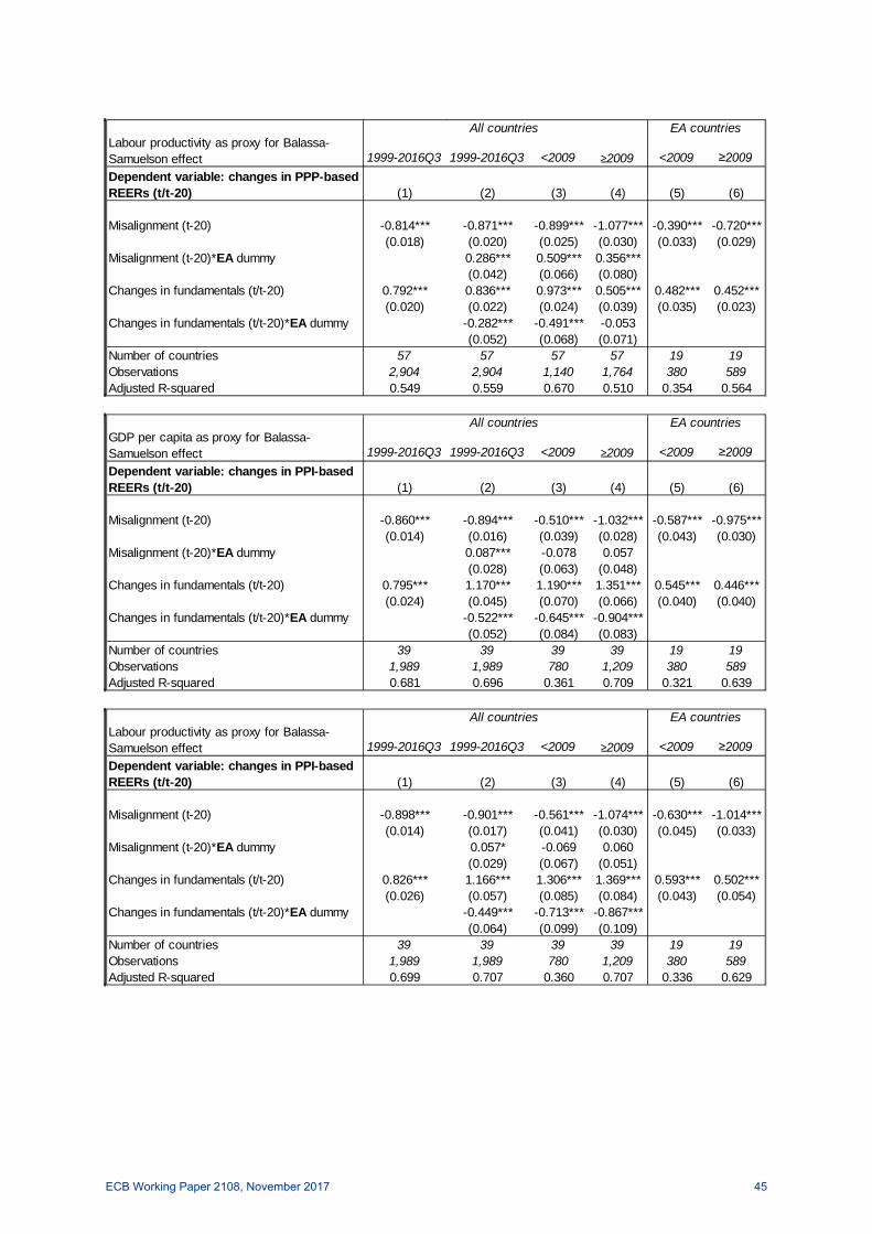
1999-2016Q3 1999-2016Q3 <2009 ≥2009 <2009 ≥2009Dependent variable: changes in PPP-based REERs (t/t-20) (1) (2) (3) (4) (5) (6)

Misalignment (t-20) -0.814*** -0.871*** -0.899*** -1.077*** -0.390*** -0.720***(0.018) (0.020) (0.025) (0.030) (0.033) (0.029)







1999-2016Q3 1999-2016Q3 <2009 ≥2009 <2009 ≥2009Dependent variable: changes in PPI-based REERs (t/t-20) (1) (2) (3) (4) (5) (6)

Misalignment (t-20) -0.860*** -0.894*** -0.510*** -1.032*** -0.587*** -0.975***(0.014) (0.016) (0.039) (0.028) (0.043) (0.030)

Misalignment (t-20)*EA dummy 0.087*** -0.078 0.057(0.028) (0.063) (0.048)


Changes in fundamentals (t/t-20)*EA dummy -0.522*** -0.645*** -0.904***(0.052) (0.084) (0.083)

Number of countries 39 39 39 39 19 19Observations 1,989 1,989 780 1,209 380 589Adjusted R-squared 0.681 0.696 0.361 0.709 0.321 0.639



1999-2016Q3 1999-2016Q3 <2009 ≥2009 <2009 ≥2009Dependent variable: changes in PPI-based REERs (t/t-20) (1) (2) (3) (4) (5) (6)

Misalignment (t-20) -0.898*** -0.901*** -0.561*** -1.074*** -0.630*** -1.014***(0.014) (0.017) (0.041) (0.030) (0.045) (0.033)

Misalignment (t-20)*EA dummy 0.057* -0.069 0.060(0.029) (0.067) (0.051)







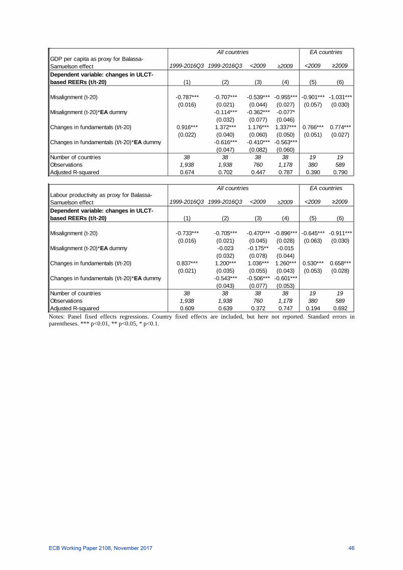
Notes: Panel fixed effects regressions. Country fixed effects are included, but here not reported. Standard errors in parentheses. *** p<0.01, ** p<0.05, * p<0.1.

1999-2016Q3 1999-2016Q3 <2009 ≥2009 <2009 ≥2009Dependent variable: changes in ULCT-based REERs (t/t-20) (1) (2) (3) (4) (5) (6)

Misalignment (t-20) -0.787*** -0.707*** -0.539*** -0.955*** -0.901*** -1.031***(0.016) (0.021) (0.044) (0.027) (0.057) (0.030)

Misalignment (t-20)*EA dummy -0.114*** -0.362*** -0.077*(0.032) (0.077) (0.046)






1999-2016Q3 1999-2016Q3 <2009 ≥2009 <2009 ≥2009Dependent variable: changes in ULCT-based REERs (t/t-20) (1) (2) (3) (4) (5) (6)

Misalignment (t-20) -0.733*** -0.705*** -0.470*** -0.896*** -0.645*** -0.911***(0.016) (0.021) (0.045) (0.028) (0.063) (0.030)

Misalignment (t-20)*EA dummy -0.023 -0.175** -0.015(0.032) (0.078) (0.044)







Table B12. The relationship between actual HCIs and real misalignments in “stressed” euro area countries: regression results according to different deflators

1999-2016Q3 <2009 ≥2009 1999-2016Q3 <2009 ≥2009Dependent variable: changes in GDP deflator-based REERs (t/t-20) (1) (2) (3) (1) (2) (3)

Misalignment (t-20) -0.452*** -0.780*** -0.288*** -0.395*** -0.733*** -0.267***(0.030) (0.053) (0.043) (0.031) (0.057) (0.049)

Misalignment (t-20)*Stressed -0.455*** -0.015 -0.600*** -0.703*** -0.102 -0.705***(0.061) (0.074) (0.089) (0.070) (0.079) (0.109)

Changes in fundamentals (t/t-20) 0.244*** 0.091** 0.190*** 0.250*** 0.080** 0.178***(0.029) (0.037) (0.024) (0.031) (0.037) (0.027)




1999-2016Q3 <2009 ≥2009 1999-2016Q3 <2009 ≥2009Dependent variable: changes in PPP-based REERs (t/t-20) (1) (2) (3) (1) (2) (3)

Misalignment (t-20) -0.454*** -0.746*** -0.257*** -0.415*** -0.709*** -0.245***(0.031) (0.047) (0.045) (0.033) (0.049) (0.052)

Misalignment (t-20)*Stressed -0.387*** -0.026 -0.584*** -0.637*** -0.111 -0.742***(0.059) (0.069) (0.087) (0.070) (0.071) (0.112)

Changes in fundamentals (t/t-20) 0.176*** 0.070** 0.098*** 0.199*** 0.062* 0.096***(0.030) (0.034) (0.025) (0.034) (0.036) (0.030)




1999-2016Q3 <2009 ≥2009 1999-2016Q3 <2009 ≥2009Dependent variable: changes in PPI-based REERs (t/t-20) (1) (2) (3) (1) (2) (3)

Misalignment (t-20) -0.904*** -0.805*** -0.808*** -0.903*** -0.710*** -0.847***(0.026) (0.078) (0.048) (0.025) (0.077) (0.049)

Misalignment (t-20)*Stressed -0.093 -0.181* -0.194** -0.154*** -0.245** -0.258***(0.063) (0.108) (0.097) (0.054) (0.103) (0.096)

Changes in fundamentals (t/t-20) -0.162*** -1.044*** -0.021 -0.522*** -1.494*** -0.238**(0.062) (0.106) (0.064) (0.091) (0.149) (0.101)

Changes in fundamentals (t/t-20)*Stressed 0.676*** 0.969*** 1.027*** 0.712*** 1.219*** 0.451**(0.109) (0.239) (0.177) (0.155) (0.256) (0.214)




Notes: Standard errors in parentheses. *** p<0.01, ** p<0.05, * p<0.1. Panel fixed effects regressions. Country fixed effects are included, but here not reported. Stressed euro area countries include all 19 euro area countries except for Austria, Belgium, Finland, France, Germany, Luxembourg, and the Netherlands.

1999-2016Q3 <2009 ≥2009 1999-2016Q3 <2009 ≥2009Dependent variable: changes in ULCT-based REERs (t/t-20) (1) (2) (3) (1) (2) (3)

Misalignment (t-20) -0.514*** -0.774*** -0.548*** -0.422*** -0.651*** -0.457***(0.037) (0.077) (0.071) (0.035) (0.080) (0.058)

Misalignment (t-20)*Stressed -0.413*** -0.133 -0.601*** -0.683*** -0.305*** -0.640***(0.068) (0.101) (0.117) (0.073) (0.109) (0.103)

Changes in fundamentals (t/t-20) 0.388*** 0.097* 0.416*** 0.314*** 0.094* 0.297***(0.043) (0.054) (0.050) (0.035) (0.048) (0.033)

Changes in fundamentals (t/t-20)*Stressed 0.674*** 0.079 0.750*** 0.981*** 0.265** 1.745***(0.063) (0.108) (0.088) (0.067) (0.108) (0.088)




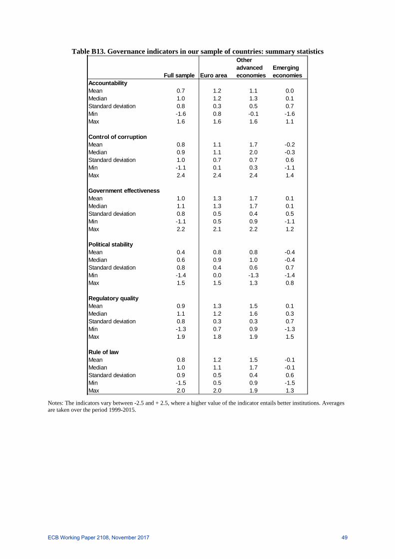
Table B13. Governance indicators in our sample of countries: summary statistics

Notes: The indicators vary between -2.5 and + 2.5, where a higher value of the indicator entails better institutions. Averages are taken over the period 1999-2015.

Full sample Euro area

Other advanced economies

Emerging economies

AccountabilityMean 0.7 1.2 1.1 0.0Median 1.0 1.2 1.3 0.1Standard deviation 0.8 0.3 0.5 0.7Min -1.6 0.8 -0.1 -1.6Max 1.6 1.6 1.6 1.1

Control of corruptionMean 0.8 1.1 1.7 -0.2Median 0.9 1.1 2.0 -0.3Standard deviation 1.0 0.7 0.7 0.6Min -1.1 0.1 0.3 -1.1Max 2.4 2.4 2.4 1.4

Government effectivenessMean 1.0 1.3 1.7 0.1Median 1.1 1.3 1.7 0.1Standard deviation 0.8 0.5 0.4 0.5Min -1.1 0.5 0.9 -1.1Max 2.2 2.1 2.2 1.2

Political stabilityMean 0.4 0.8 0.8 -0.4Median 0.6 0.9 1.0 -0.4Standard deviation 0.8 0.4 0.6 0.7Min -1.4 0.0 -1.3 -1.4Max 1.5 1.5 1.3 0.8

Regulatory qualityMean 0.9 1.3 1.5 0.1Median 1.1 1.2 1.6 0.3Standard deviation 0.8 0.3 0.3 0.7Min -1.3 0.7 0.9 -1.3Max 1.9 1.8 1.9 1.5

Rule of lawMean 0.8 1.2 1.5 -0.1Median 1.0 1.1 1.7 -0.1Standard deviation 0.9 0.5 0.4 0.6Min -1.5 0.5 0.9 -1.5Max 2.0 2.0 1.9 1.3


References

Abiad, A., Kannan, P., and Lee, J. (2009), “Evaluating Historical CGER Assessments: How Well Have They Predicted Subsequent Exchange Rate Movements?”, IMF Working Papers 32.

Adler, K. and Grisse, C. (2014), “Real exchange rates and fundamentals: robustness across alternative model specifications”, SNB Working Papers 7/2014.

Ahn, J.B., Mano, R. and Zhou, J. (2017), “Real exchange rate and external balance: How important are price deflators?”, IMF Working Papers 17/81.

Alberola, E., Cervero, S. G., Lopez, H. and Ubide, A. (2002), “Quo vadis euro?”, European Journal of Finance 8(4), pp. 352–70.

Alesina, A. and Wagner, A.F. (2006), “Choosing (and reneging on) exchange rate regimes”, Journal of the European Economic Association 4(4), pp. 770–799.

Altissimo, F., Ehrmann, M. and Smets, F. (2006), “Inflation persistence and price-setting in the euro area. A summary of the IPN evidence”, ECB Occaional Papers 46.

Angeloni, I. and Ehrmann, M. (2007), “Euro area inflation differentials”, The B.E. Journal of Macroeconomics, Topics, 7(1), article 24.

Balassa, B. (1964), “The Purchasing Power Parity Doctrine: A Reappraisal”, Journal of Political Economy 72(6), pp. 584-96.

Baldwin, R. E. (2006), In or Out: Does It Matter? An Evidence-Based Analysis of the Euro’s Trade Effects, Centre for Economic Policy Research: London.

Beck, G.W., Hubrich, K., and Marcellino, M. (2009), “Regional inflation dynamics within and across euro area countries and a comparison with the United States”, Economic Policy, pp. 141–184.

Bénassy-Queré, A., Béreau, S. and Mignon, V. (2009), “Robust estimations of equilibrium exchange rates within the G20: A panel BEER approach”, Scottish Journal of Political Economy 56(5), pp. 608-633.

Bergin, P.R., Glick, R. and Taylor, A.M. (2006), “Productivity, tradability, and the long-run price puzzle”, Journal of Monetary Economics 53, pp. 2041-2066.

Bergin, P., Glick, R. and Wu, J. (2014), “Mussa redux and conditional PPP”, Journal of Monetary Economics 68, pp. 101-114.

Bergin, P., Glick, R. and Wu, J. (2017), “Conditional PPP and real exchange rate convergence in the euro area”, Journal of International Money and Finance, forthcoming.

Berka, M., Devereux, M. and Engel, C. (2012), “Real exchange rate adjustment in and out of the Eurozone”, American Economic Review 102, pp. 179-185.

Berka, M., Devereux, M. and Engel, C. (2014), “Real exchange rates and sectoral productivity in the Eurozone”, NBER Working Papers 20510.

Bissoondeeal, R. K. (2008), “Post-Bretton Woods evidence on PPP under different exchange rate regimes”, Applied Financial Economics 18, pp. 1481–1488.

Broadberry, S.N., Giordano, C. and Zollino, F. (2013), “Productivity” in Toniolo, G. (ed.), The Oxford Handbook of the Italian Economy since Unification, New York: Oxford University Press.

Broz, J.L., Frieden, J. and Weymouth, S. (2008), “Exchange Rate Policy Attitudes: Direct Evidence from Survey Data”, IMF Staff Papers 55(3), pp.417-444.

Bussière, M., Ca’Zorzi, M., Chudik, A. and Dieppe, A. (2010), “Methodological Advances in the Assessment of Equilibrium Exchange Rates”, ECB Working Papers 1151.

Cheung, Y. W., Chinn, M. D. and Fujii, E. (2010) ‘Measuring Renminbi Misalignment: Where Do We Stand?’, Hong Kong Institute for Monetary Reserve Working Paper 24/2010.

Cheung, Y-W, Chinn, M.D., Pascual, A.G. and Zhang, Y. (2017), “Exchange rate prediction redux: new models, new data, new currencies”, NBER Working Papers 23267.

Chinn, M.D. (1999), “Productivity, government spending and the real exchange rates: evidence for OECD countries”, in MacDonald, R. and Stein, J.L. (eds.), Equilibrium exchange rates, Kluwer Academic Publisher: UK, pp. 163-190.

Chinn, M.D. (2006), “A Primer on Real Effective Exchange Rates: Determinants, Overvaluation, Trade Flows and Competitive Devaluation”, Open Economies Review 17, pp. 115-143.

Choi, W.J. and Taylor, A.M. (2017), “Precaution vs. mercantilism: reserve accumulation, capital controls, and the real exchange rate”, CEPR Discussion Papers 11963.


Christiansen, L., Prati, A. Ricci, L.A. and Tressel, T. (2009), “External Balance in Low-Income Countries”, in Reichlin, L. and West, K. (eds.), NBER International Seminar on Macroeconomics 2009, University of Chicago Press.

Christodoulopoulou, S. and Tkačevs, O. (2014), “Measuring the effectiveness of cost and price competitiveness in external rebalancing of euro area countries: What do alternative HCIs tell us?”, ECB Working Papers1736.

Clark, P.B. and MacDonald, R. (1998), “Exchange Rates and Economic Fundamentals: A Methodological Comparison of BEERs and FEERs”, IMF Working Papers 98/67.

Cline, W. R. and Williamson, J. (2010), “Estimates of Fundamental Equilibrium Exchange Rates”, Peterson Institute for International Economics Policy Brief 15.

Comunale, M. (2015), “Long-run determinants and misalignments of the real effective exchange rate in the EU”, Lietuvos Bankas Working Papers 18.

Comunale, M. (2017), “Dutch disease, real effective exchange rate misalignments and their effect on GDP growth in EU”, Journal of International Money and Finance 73, pp. 350-370.

Coudert, V. and Couharde, C. (2009), “Currency misalignments and exchange rate regimes in emerging and developing economies”, Review of International Economics 17(1), pp. 121-136.

Coudert, V., Couharde, C. and Mignon, V. (2013), “On Currency Misalignments within the Euro Area”, Review of International Economics 21(1), pp. 35-48.

Deaton, A. and Heston, A.A. (2010), “Understanding PPPs and PPP-based national accounts”, American Economic Journal of Macroeconomics 2, pp. 1-35.

De Gregorio, J., Giovannini, A. and Krueger, T.K. (1994), “The Behaviour of Nontradable Goods in Europe: Evidence and Interpretation”, Review of International Economics 2, pp. 284-305.

De Gregorio, J., Giovannini, A. and Wolf, H. (1994), “International evidence on tradables and nontradables inflation”, European Economic Review 38(6), pp. 1225-1244.

De Gregorio, J. and Wolf, H. (1994), “Terms of Trade, Productivity and the Real Exchange Rate”, NBER Working Papers 4807.

De Haan, J. (2010), “Inflation Differentials in the Euro Area: A Survey”, in de Haan, J. and Berger, H. (eds.), The European Central Bank at Ten, Springer: Berlin, pp. 11-33.

Devereux, M. B. (1999), “Real Exchange Rate Trends and Growth: A Model of East Asia”, Review of International Economics 7(3), pp. 509–521.

Dubas, J.M. (2009), “The importance of the exchange rate regime in limiting misalignment”, World Development 37(10), pp. 1612-1622.

Eberhardt, M. (2012), “Estimating panel time-series models with heterogeneous slopes”, The Stata Journal 12(1), pp. 61-71.

ECB (2015), “Update of trade weights data underlying the EERs and HCIs”, 3 August, available at https://www.ecb.europa.eu/stats/exchange/effective/html/index.en.html.

El-Shagi, M., Lindner, A. and von Schweinitz, G. (2016), “Real Effective Exchange Rate Misalignment in the Euro Area: A Counterfactual Analysis”, Review of International Economics 24(1), pp. 37–66.

Engel, C. (1999), “Accounting for U.S. Real Exchange Rate Changes”, Journal of Political Economy 107(3), pp. 507-538.

Engel, C. and Rogers, J.H. (2004), “European product market integration after the euro”, Economic Policy 19, pp. 347-384.

Fischer, C. and Hossfeld, O. (2014), “A Consistent Set of Multilateral Productivity Approached-Based Indicators of Price Competitiveness”, ECB Working Papers 1706.

Flood, R.P. and Rose, A.K. (1999), “Understanding exchange rate volatility without the contrivance of macroeconomics”, Economic Journal 109, pp. 660-672.

Franks, J., Barkbu, B., Blavy, R., Oman, W. and Schoelermann, H. (2017), “Economic Convergence in the Euro Area: Coming Together or Drifting Apart?”, IMF Working Paper, forthcoming.

Friedman, M. (1953), Essays in Positive Economics, Chicago: University of Chicago.

Froot, K. A., and Rogoff, K. (1992), "Government Consumption and the Real Exchange Rate: The Empirical Evidence", Harvard University mimeo.

Froot, K.A. and Rogoff, K. (1994), “Perspectives on PPP and Long-Run Real Exchange Rates”, NBER Working Papers 4952.

Gamberoni, E., Gartner, C., Giordano, C. and Lopez-Garcia, P. (2016), “Is corruption efficiency-enhancing? A case study of nine Central and Eastern European countries”, ECB Working Papers 1950.


https://www.ecb.europa.eu/stats/exchange/effective/html/index.en.html

Gamberoni, E., Giordano, C. and Lopez-Garcia, P., (2016), “Capital and labour (mis) allocation in the euro area: some stylized facts and determinants”, Bank of Italy Occasional Papers 349.

Gandolfo, G. and Felettigh, A. (1998), “The NATREX: An Alternative Approach. Theory and Empirical Verifications,” University “La Sapienza” Working Papers 52.

Gandolfo, G., Padoan, P.C. and de Arcangelis, G. (1993), “The theory of exchange rate determination and exchange rate forecasting” in Frisch, H. and Wörgötter, A. (eds.), Open-Economy Macroeconomics, Proceedings of a conference held in Vienna by the International Economic Association, MacMillan.

Giordano, C. and Zollino, F. (2016), “Shedding Light on Price- and Non-price competitiveness Determinants of Foreign Trade in the Four Largest Euro area Countries”, Review of International Economics 24(3), pp. 604-634.

Giordano, C., Toniolo, G. and Zollino, F. (2017), “Long-run trends in Italian productivity”, Banca d’Italia Occasional Papers, forthcoming.

Gnimassoun, B. and Mignon, V. (2015), “Persistence of Current-account Disequilibria and Real Exchange-rate Misalignments”, Review of International Economics 23(1), pp. 137-159.

Goldfajn, I. and Valdes, R.O. (1999), “The aftermath of appreciations”, Quarterly Journal of Economics 114, pp. 229-262.

Hajek, J. (2016), “Real Exchange Rate Misalignment in the Euro Area: Is the Current Development Helpful?”, IES Working Papers 11.

Hassan, F. (2016), “The Price of Development: The Penn-Balassa-Samuelson Effect Revisited”,Journal of International Economics 102, pp. 291–309.

Hinkle, L., and Montiel, P. (1999), Exchange Rate Misalignment: Concepts and Measurement for Developing Countries, Oxford: Oxford University Press.

Holtemöller, O. and Mallick, S. (2013), “Exchange rate regime, real misalignment and currency crises”, Economic Modelling 34, pp. 5-14.

Hossfeld, O. (2010), “Equilibrium real effective exchange rates and real exchange rate misalignments: Time series vs. panel estimates”, FIW Working Papers 65.

Housklova, J. and Osbat, C. (2009), “Panel cointegration approaches to estimating equilibrium real exchange rates – separating the wheat from the chaff”, mimeo.

Huang, C.-H. and Yang, C.-Y. (2015), “European exchange rate regimes and purchasing power parity: An empirical study on eleven eurozone countries”, International Review of Economics and Finance 35, pp. 100–109.

ICP (2007), ICP Methodological Handbook, The World Bank: Washington D.C.

Im, K., Pesaran, M.H., and Shin, Y. (1995), “Testing for Unit Roots in Heterogeneous Panels”, DAE Working Papers Amalgamated Series 9526, University of Cambridge.

Imbs, J., Mumtaz, H., Ravn, M. O. and Rey, H. (2002), “PPP strikes back: Aggregation and the real exchange rate”, NBER Working Paper 9372.

Isard, P. (2007) “Equilibrium Exchange Rates: Assessment Methodologies”, IMF Working Papers 226.

Kao, C. and Chiang, M.H. (2000), “On the estimation and inference of a cointegrated regression in panel data”, in Baltagi, B. and Kao, C. (eds.), Advances in econometrics vol. 15, pp. 179-222.

Kapetanios, G., Pesaran, M.H. and Yamagata, T. (2006), “Panels with Nonstationary Multifactor Error Structures”, IZA Discussion Papers 2243.

Kessler, M. and Subramanian, A. (2014), “Is the Renminbi still Undervalued? Not According to New PPP Estimates”, Vox-Eu, May 1.

Kilian, L. and Zha, T. (2002), “Quantifying the Uncertainty about the Half-Life of Deviations from PPP”, Journal of Applied Econometrics 17(2), pp.107-125.

Kravis, I.B., Heston, A. W. and Summers, R. (1978), “Real GDP Per Capita for More Than One Hundred Countries”, The Economic Journal 88(350), pp. 215-242.

Lane, P.R. (2006), “The Real Effects of European Monetary Union”, Journal of Economic Perspectives 20(4), pp. 47-66.

Lane, P. R. and Milesi-Ferretti, G.M. (2002), “External wealth, the trade balance and the real exchange rate”, European Economic Review 46(6), pp. 1049-1071.

Lane, P. R. and Milesi-Ferretti, G.M. (2004), “The Transfer Problem Revisited: Net Foreign Assets and Real Exchange Rates”, The Review of Economics and Statistics 86(4), pp. 841-857.

Lee, J., Milesi-Ferretti, G.M., Ostry, J., Prati, A. and Ricci, L.A. (2008), “Exchange Rates Assessments: CGER Methodologies”, IMF Occasional Papers 261.


Lothian, J. and Taylor, M. (2008), “Real Exchange Rates Over the Past Two Centuries: How Important is the Harrod-Balassa-Samuelson Effect?”, The Economic Journal 118, pp. 1742-63.

Maeso Fernández, F., Osbat, C. and Schnatz, B. (2001), “Determinants of the Euro Real Effective Exchange Rate: A BEER/PEER Approach”, ECB Working Papers 85.

Maeso Fernández, F., Osbat, C. and Schnatz, B. (2004), “Towards the Estimation of Equilibrium Exchange Rates for CEE Acceding Countries: Methodological Issues and a Panel Cointegration Perspective”, ECB Working Papers 353.

Mancini-Griffolo, T., Meyer, C., Natal, J-M and Zanetti, A. (2014), "Determinants of the Swiss franc real exchange rate", SNB Working Paper 08/2014.

Meese, R.A. and Rogoff, K. (1983a), “Empirical exchange rate models of the Seventies: Do they fit out of sample?”, Journal of International Economics 14, pp. 3-24.

Meese, R.A. and Rogoff, K. (1983b), “The out-of-sample failure of empirical exchange rate models: sampling error or mis-specification?”, in Frenkel, J.A. (ed.), Exchange Rates and International Macroeconomics, Chicago: University of Chicago Press.

Melecký, M. and Komárek, L. (2007), “The behavioural equilibrium exchange rate of the Czech Koruna”, Transition Studies Review 14, pp. 105-121.

Mussa, M. (1986), “Nominal Exchange Rate Regimes and the Behaviour of Real Exchange Rates: Evidence and Implications”, Carnegie-Rochester Conference Series on Public Policy 25, pp. 117-214.

Neary, P. (1988), “Determinants of the equilibrium real exchange rate”, American Economic Review 78(1), pp. 210-215.

Nouira, R. and Sekkat, K. (2015), “What determines the extent of real exchange rate misalignment in developing countries?”, International Economics 141, pp. 135-151.

Obstfeld, M. and Rogoff, K (1996), Foundations of International Macroeconomics, Cambridge, Mass.: MIT Press.

Obstfeld, M. and Rogoff, K (2001), “The Six Major Puzzles in International Macroeconomics: Is There a Common Cause?”, in Bernanke, B. and Rogoff, K. (eds.), NBER Macroeconomics Annual 2000, Volume 15, pp. 339-412.

Papell, D.H. and Prodan, R. (2006), “Additional evidence of long-run purchasing power parity with restricted structural change”, Journal of Money, Credit and Banking 38, pp. 1329-1349.

Parsley, D. C., and Popper, H. A. (2001), “Official exchange rate arrangements and real exchange rate behaviour”, Journal of Money, Credit and Banking 33, pp. 976–993.

Pesaran, M.H. (2006), “Estimation and Inference in Large Heterogeneous Panels with a Multifactor Error Structure”, Econometrica 74(4), pp. 967–1012.

Pesaran, M.H. (2007), “A Simple Panel Unit Root Test in the Presence of Cross-Section Dependence”, Journal of Applied Econometrics 22(2), pp. 265–312.

Phillips, S., Catao, L., Ricci, L., Bems, R., Das, M., Di Giovanni, J., Unsal, D.F., Castillo, M., Lee, J., Rodriguez, J. and Vargas, M. (2013), “The External Balance Assessment (EBA) methodology”, IMF Working Paper 13.

Reinhart, C.M. and Rogoff, K.S. (2004), “The modern history of exchange rate arrangements: a reinterpretation”, Quarterly Journal of Economics 119, pp. 1-48.

Ricci, L.A., Milesi-Ferretti, G.M. and Lee, J. (2013), “Real exchange rates and fundamentals: a cross-country perspective”, Journal of Money, Credit and Banking 45, pp. 845-65.

Rogoff, K. (1996), “The Purchasing Power Parity puzzle”, Journal of Economic Literature 34, pp. 647-668.

Rodrik, D. (2008), “The Real Exchange Rate and Economic Growth”, Brookings Papers on Economic Activity, pp. 365-412.

Rose, A.K. (2000), “One money, one market: The effect of common currencies on trade”, Economic Policy: A European Forum 30, pp. 7-33.

Rose, A.K., Supaat, S. and Braude, J. (2009), “Fertility and the real exchange rate”, Canadian Journal of Economics 42(2), pp. 496-518.

Salto, M. and Turrini, A. (2010), “Comparing alternative methodologies for real exchange rate assessment”, European Economy Economic Papers 427.

Samuelson, P. (1964), “Theoretical Notes on Trade Problems”, Review of Economics and Statistics 46, pp. 145-154.

Shambaugh, J.C. (2004), “The Effect of Fixed Exchange Rates on Monetary Policy”, The Quarterly Journal of Economics 119(1), pp. 301-352.

Schmitz, M., De Clercq, Fidora, M., Lauro, B. and Pinheiro, C. (2012), “Revisiting the effective exchange rates of the euro”, ECB Occasional Papers 134.


Schnatz, B. (2011), “Global imbalances and the pretence of knowing fundamental equilibrium exchange rates”, Pacific Economics. Review 16 (5), pp. 604–615.

Schnatz, B., Vijselaar, F. and Osbat, C. (2003), “Productivity and the “synthetic” euro-dollar exchange rate”, ECB Working Papers 225.

Siregar, R.Y. and Rajan, R. (2006), “Model of Equilibrium Real Exchange Rates Revisited: A Selective Review of the Literature,” University of Adelaide Discussion Papers 604.

Stein, J. (1990), “The Real Exchange Rate”, Journal of Banking and Finance 14(5), pp. 1045-78.

Stock, J. and Watson, M. (1993), “A simple estimate of cointegrating vectors in higher order integrated systems”, Econometrica 61(4), pp. 783-820.

Taylor, A. (2002), “A century of purchasing-power parity”, Review of Economics and Statistics 84, pp. 139-154.

Taylor, A. and Taylor, M. (2004), “The Purchasing Power Parity Debate”, Journal of Economic Perspectives 18(4), pp. 135-158.

Taylor, M. (2006), “Real exchange rates and Purchasing Power Parity: mean-reversion in economic thought”, Applied Financial Economics 16, pp. 1-17.

Timmer, M.P., Inklar, R. and O’Mahony, M. (eds.) (2010), Economic Growth in Europe: A Comparative Industry Perspective, Cambridge, Mass.: Cambridge University Press.

Williamson, J. (1994), “Estimates of FEERs” in Williamson, J. (ed.), Estimating Equilibrium Exchange Rates, Institute for International Economics.

Wren-Lewis, S. (1992), “On the Analytical Foundations of the Fundamental Equilibrium Exchange Rate”, in Hargreaves, C. P. (ed.), Macroeconomic Modeling of the Long Run, London: E. Elgar.

Yamagata, T. (2011), “Panels with non-stationary multifactor error structures”, Journal of Econometrics 160(2), pp. 326-348.


http://www.tandfonline.com/toc/rafe20/16/1-2

http://www.tandfonline.com/toc/rafe20/16/1-2

Acknowledgements We are grateful to Christoph Ellermann and Rebekka Bellmann for excellent research assistance. We thank an anonymous referee, Nektarios Aslanidis, Mariarosaria Comunale, Riccardo De Bonis, Valerio Della Corte, Juan Luis Diaz del Hoyo, Ettore Dorrucci, Silvia Fabiani, Alberto Felettigh, Jorgo Georgiadis, Federic Holm-Hadulla, Pavlos Karadeloglou, Hans-Joachim Klöckers, Klaus Masuch, Giacomo Oddo, Chiara Osbat, Peter Praet, Frank Smets, Livio Stracca, Cédric Tille and Bernhard Winkler, as well as participants at ECB seminars and at the ICMAIF 2017 conference, INFINITI conference 2017, EEA annual congress 2017 and XXIV Villa Mondragone International Economic Seminar for highly valuable suggestions and comments. Any error is the responsibility of the authors. The views expressed herein are those of the authors and not of their institutions.

Michael Fidora European Central Bank, Frankfurt am Main, Germany; email: [email protected]

Claire Giordano Banca d’Italia, Rome, Italy; email: [email protected]

Martin Schmitz European Central Bank, Frankfurt am Main, Germany; email: [email protected]

© European Central Bank, 2017

Postal address 60640 Frankfurt am Main, Germany Telephone +49 69 1344 0Website www.ecb.europa.eu

All rights reserved. Any reproduction, publication and reprint in the form of a different publication, whether printed or produced electronically, in whole or in part, is permitted only with the explicit written authorisation of the ECB or the authors.

This paper can be downloaded without charge from www.ecb.europa.eu, from the Social Science Research Network electronic library or from RePEc: Research Papers in Economics. Information on all of the papers published in the ECB Working Paper Series can be found on the ECB’s website.

ISSN DOI ISBN

1725-2806 (pdf)978-92-899-2830-4 (pdf) EU catalogue No

10.2866/96117 (pdf)QB-AR-17-120-EN-N (pdf)

mailto:[email protected]



http://www.ecb.europa.eu/

http://www.ecb.europa.eu/

http://ssrn.com/

https://ideas.repec.org/s/ecb/ecbwps.html

http://www.ecb.europa.eu/pub/research/working-papers/html/index.en.html

Working Paper Series - European Central Bank · Working Paper Series . Real exchange rate...

Documents

Transcript of Working Paper Series - European Central Bank · Working Paper Series . Real exchange rate...