Working Paper Series · 2018-11-20 · Working Paper Series . Credit supply and demand in...

Working Paper Series Credit supply and demand in unconventional times

Carlo Altavilla, Miguel Boucinha, Sarah Holton, Steven Ongena

Disclaimer: This paper should not be reported as representing the views of the European Central Bank (ECB). The views expressed are those of the authors and do not necessarily reflect those of the ECB.

No 2202 / November 2018

Abstract

Do borrowers demand less credit from banks with weak balance sheet positions? To

answer this question we use novel bank-specific survey data matched with confidential balance

sheet information on a large set of euro area banks. We find that, following a conventional

monetary policy shock, bank balance sheet strength influences not only credit supply but

also credit demand. The resilience of lenders plays an important role for firms when selecting

whom to borrow from. We also assess the impact on credit origination of unconventional

monetary policies using survey responses on the exposure of individual banks to quantitative

easing and negative interest rate policies. We find that both policies do stimulate loan

supply even after fully controlling for bank-specific demand, borrower quality, and balance

sheet strength.

JEL: E51, G21.

Keywords: credit demand and supply, bank lending survey, balance sheet strength, non-

standard monetary policy

ECB Working Paper Series No 2202 / November 2018 1

Non-technical summary

The conventional wisdom in banking literature is that balance sheet characteristics of finan-

cial intermediaries influence their ability to supply credit to households and firms. Weak banks

tend to originate less credit. This paper studies whether weak banks also face less demand,

owing to borrowers diverting their demand for credit towards banks with more solid balance

sheets. We address this thus far neglected question using a novel dataset of individual banks’

responses on their credit supply and demand conditions linked to their balance sheets. Under-

standing the transmission of shocks to the real economy via banks and accounting for credit

demand is vital when accurately assessing the impact of monetary policies. With this in mind,

we additionally analyse how the strength of this “demand channel” interacts with conventional

and unconventional monetary policy measures.

We contribute to the literature in a number of ways. The so-called “bank lending channel”

literature is devoted to identifying the effects of credit supply shocks, controlling for possible

changes in demand, using assumptions of varying strength. We assess the validity of some

of these assumptions using demand directly reported by individual banks. There are papers

suggesting that firms’ credit demand may not be homogenous across banks owing to bank

specialisation, location or even quality. We extend on this literature by examining whether

changes in monetary policy have a differential effect on demand owing to banks’ resilience. In

addition, we contribute to the literature concerned with assessing the effects of unconventional

monetary policies on lending by exploring survey responses on the exposure of individual banks

to quantitative easing and negative interest rate policies and controlling for the demand they

face.

We find that, following a conventional monetary policy shock, bank balance sheet strength

influences not only credit supply but also credit demand. The resilience of lenders plays an

important role for firms when selecting whom to borrow from. With respect to the effect of

unconventional monetary policies on lending, we find that both quantitative easing and the neg-

ative interest rate policy stimulated loan supply, even when taking into account bank-specific

demand, the quality of the borrower pool, and balance sheet strength. We provide confirma-

tion of the hypothesised channels of each policy by showing that banks with higher sovereign

bond holdings extended more credit following the announcement of the quantitative easing pro-

gramme and that banks with higher excess liquidity holdings had stronger credit flows after the

introduction of negative deposit facility rates.


1 Introduction

The conventional wisdom in the banking literature is that balance sheet characteristics of finan-

cial intermediaries influence their ability to supply credit to households and firms (e.g., Kashyap

and Stein (2000)). In a time of monetary contraction, for example, weak banks will tend to grant

less credit. In this paper we study whether weak banks may also face less demand, as borrowers

might concurrently divert their demand for credit towards banks with more solid balance sheet

positions in order to avoid having to deal with a constrained bank or even - in bankruptcy -

with a bank receiver. We show that the impact of a standard monetary policy shock on credit

demand varies across banks depending on their resilience, and using this measure of bank spe-

cific demand, we estimate the impact of non-standard monetary policy measures specifically on

bank credit supply.

Understanding the transmission of shocks to the real economy via banks is of utmost impor-

tance as optimal policy responses depend on whether credit developments are driven by changes

in banks’ willingness to lend or in borrowers’ propensity to invest or consume. There is a large

literature, known as the “bank lending channel”,1 concerned with identifying how credit supply

shocks can vary across different types of banks by controlling for possible changes in demand

using assumptions of varying strength. A topic that has received much less attention is whether

credit demand can also vary across banks depending on their characteristics. We disentangle

the role of supply and demand in determining credit dynamics using two main ingredients: a

proxy for monetary policy shocks and an indicator of bank-specific credit demand conditions.

For both we rely heavily on a novel dataset of individual euro area credit institutions Bank

Lending Survey (iBLS) responses, which provides bank specific information on credit supply,

demand and the impact of monetary policy. By linking individual banks’ responses on how they

are affected by the negative deposit facility rate and the quantitative easing programme to hard

data on their loans and other key balance sheet variables, and effectively controlling for credit

demand they face, we can quantify the effects of these policy measures on credit provision during

these recent unconventional years.

The Bank Lending Survey (BLS) was established to complement hard data on lending flows

with information on supply and demand conditions and there is a large literature using this

survey to analyse the determinants of credit growth. As banks report specifically on how, and

why, loan supply and demand pressures are changing, survey data can provide a cleaner identifi-

1See for instance, Bernanke and Blinder (1992), Kashyap and Stein (2000), Jiménez, Ongena, Peydró and

Saurina (2012).


cation of the drivers of credit developments, without the need for assumptions on demand. Past

literature shows that survey measures of credit supply and demand have significant explanatory

power for aggregate credit and economic developments in the US (Lown and Morgan (2006)), the

euro area (de Bondt, Maddaloni, Peydró and Scopel (2010)) and for individual countries (see for

instance, Blaes (2011) for Germany and Del Giovane, Eramo and Nobili (2011) for Italy). More-

over, survey evidence shows that the transmission of monetary policy can change, in particular

during periods of stress (Ciccarelli, Maddaloni and Peydró (2013); Altavilla, Darracq Pariès and

Nicoletti (2015)), and that monetary policy shocks can be amplified through the bank lending

channel (Ciccarelli, Maddaloni and Peydró (2015)).

This paper adds to the broader bank lending channel literature concerned with identifying

the effects of credit supply shocks, by controlling for possible changes in demand. This litera-

ture employs a wide range of methodologies based on different assumptions regarding demand.

Kashyap and Stein (2000) show that lending activity responds differently to a monetary policy

shock depending on banks’ liquidity; by assuming that demand is not systematically different

across banks according to their liquidity position, they attribute this variation to supply. How-

ever, the possibility that firms that are more affected by certain shocks also tend to be customers

of the more affected banks (i.e., they are not randomly sorted across banks), may cast doubt

on the validity of this assumption and has led to the use of more granular data. For instance,

by using firm “clusters”, across characteristics such as industry, location, size and/or risk, and

by assuming that credit demand is generally homogenous within these clusters, variation in

lending across different types of banks can then be attributed to supply (Popov and Van Horen

(2015); Acharya, Eisert, Eufinger and Hirsch (2017); Degryse, De Jonghe, Jakovljevic, Mulier

and Schepens (2018)). The most rigorous identification strategy uses credit exposure data at

the bank-firm level and controls for changes in demand at the individual borrower level by using

firm-time fixed effects, which in the literature is by now widely known as using a Khwaja and

Mian (2008) type estimation strategy. The implementation of this strategy is based on firms

that have multiple bank relationships, under the assumption that any change in lending to the

same firm by different banks is driven by changes in credit supply.

There are two possible caveats even with these rich granular data methods to identify supply.

As shown in Degryse, De Jonghe, Jakovljevic, Mulier and Schepens (2018),2 the characteristics

of firms with multiple lending relationships tend to differ from those with single relationships

2For a data set of recent Belgian bank-firm exposures, they compare estimates of bank supply shocks derived

using firm cluster (industry-location-size) — time fixed effects and those using firm-time fixed effects and find that

despite these differences the estimates obtained under each method are similar.


(the former tend to be older and bigger) and the credit supply measure derived using only the

sample of multiple-bank firms is substantially different from the one derived using also single-

bank firms. Secondly, it is possible that demand can vary, not just at the firm level, but also at

the bank-firm level, which can complicate the identification of supply shocks using firm time fixed

effects. Past literature has highlighted a number of factors that might influence a firm’s choice

of bank, such as bank proximity (Degryse and Ongena (2005)), size (Berger and Udell (2002),

Berger et al. (2005)), specialisation (Paravisini, Rappoport and Schnabl (2014), Paravisini,

Rappoport, Schnabl and Wolfenzon (2015)) and capital position (Holmstrom and Tirole (1997),

Schwert (2018)). In line with the latter literature, Khwaja and Mian (2008) acknowledged that a

potential problem with their approach is that it fails to capture “strategic withdrawal” by firms

from banks with balance sheet problems for fear that the bank will become insolvent. There is

even evidence that borrowers may be willing to pay for bank capital strength (Kim, Kristiansen,

Vale, 2005). Anticipating the possibility of bank insolvency, bank-dependent firms may match

with well capitalized banks, while firms with access to the bond market might borrow from

banks with less capital (Schwert, 2018)3. Such matching of bank-dependent firms with stable

banks smooths cyclicality in aggregate credit provision and mitigates the effects of bank shocks

on the real economy. In order to shed light on the relevance of these concerns and account for

firm — bank matching outcomes, we use banks’ own reported credit demand from the BLS.

A number of existing theories imply that credit demand should be higher for more resilient

banks. First, firms may want to align themselves with stronger banks in order to signal their

quality. Billett, Flannery and Garfinkel (1995) find strong evidence that loan announcements

with higher quality lenders are associated with significantly higher abnormal returns to the

firm’s stock price, implying that a loan from a strong bank conveys more positive information

about the borrower’s prospects. Second, as already mentioned, banks with stronger balance

sheets are capable of maintaining loan growth when faced with a shock, such as a contraction in

monetary policy (Kishan and Opiela, 2000; Kashyap and Stein, 2000; Gambacorta and Mistrulli,

2004). Third, models of relationship lending show that firms cannot seamlessly communicate

information that banks obtain about them over the course of a relationship to other outside

banks. Therefore, firms that need to switch banks (either owing to bank credit constraints or

collapse) could pay a higher interest rate (Sharpe (1990) and Rajan (1992)). In order to avoid

such a fate, we posit that demand at more sound banks will in general be higher, as firms try

3Another well-documented matching is that large and physically remote firms may borrow from centralized

“large” banks that rely on hard information (Stein (2002); Petersen and Rajan (2002); Cole, Goldberg and White

(2004); Berger, Miller, Petersen, Rajan and Stein (2005)).


to establish and maintain relationships with more resilient institutions.

We also contribute to the literature on the effects of non-standard monetary policy on credit.

Previous results on the link between large scale asset purchase programmes and bank lending

include, among others, Bowman, Cai, Davies and Kamin (2015) for Japan, Rodnyansky and

Darmouni (2017) for the US and Joyce and Spaltro (2014) for the UK. In general these studies

provide evidence of a significant impact of Quantitative Easing (QE) on bank lending. In

the same vein, evidence for the euro area suggests that the ECB’s asset purchase programme

(henceforth, APP) led to a significant decline in lending rates and to an increase in credit

to the private sector (Altavilla, Giannone and Lenza (2016); Albertazzi, Becker and Boucinha

(2018)). Existing evidence on the effect of the introduction of negative interest rates is less clear.

Demiralp, Eisenschmidt and Vlassopoulos (2017) and Bottero et al. (2018) for example find a

positive effect on the supply of loans, by comparing banks with different levels of excess liquidity

holdings and different amounts of interbank loans respectively. At the same time, recent studies

document a possible impact of the negative deposit facility rate (henceforth DFR) on banks’ risk

taking. Nucera, Lucas, Schaumburg and Schwaab (2017) find that the impact of the introduction

of negative interest rates on bank risk is moderate, despite some heterogeneity across business

models, with banks relying more on deposit funding being perceived by the market as more

risky. Based on data for syndicated loans, Heider, Saidi and Schepens (2017) find that banks

with higher deposit ratios increase risk-taking by relatively more following the introduction

of the negative DFR, suggesting that banks whose margin is more negatively affected by the

policy can try to recoup profitability by increasing risk-taking. In parallel, Arce, García-Posada,

Mayordomo and Ongena (2018) find that banks whose net interest income is negatively affected

by the introduction of the negative DFR, and who are more capital constrained, react by applying

relatively stricter terms and conditions for the approval of loans, which is consistent with an

attempt to increase the regulatory capital ratio by decreasing risk weights.

Our findings provide important contributions to all these branches of the literature. Firstly,

we show that both credit supply and demand are important determinants of credit volume and

that, in line with previous studies, supply is more relevant during crisis periods. Secondly, we

show evidence that not only loan supply, but also demand can vary across banks depending on

their strength. Finally, using the measure of demand as reported by banks for identification, we

show that quantitative easing and the negative deposit facility supported loan supply.

The paper proceeds as follows. Section 2 provides an overview of the dataset and some

stylised facts. Section 3 outlines the main empirical findings on how credit growth is influenced

by demand and supply and on the impact of unconventional monetary policies on banks’ lending


behaviour. Section 4 concludes.

2 Data and Stylised Facts

This section summarises the data used in the empirical analysis and provides an overview of

developments in bank lending, credit supply, credit demand, and the possible impact of uncon-

ventional monetary policies. Individual banks’ BLS responses on the unconventional measures

are particularly useful as they provide a direct measure of exposure to the specific policy shocks

and therefore should not in principle be confounded by any other concurrent event.

2.1 Lending activity, credit supply and demand

Our main source of data is a novel confidential data set on iBLS — a survey containing self-

reported information on banks’ credit supply and demand developments. Our dataset contains

quarterly information from 2002Q4 to 2017Q4 on supply and demand conditions in credit mar-

kets for an unbalanced panel of 116 banks across 13 countries in the euro area.4 We match

this dataset with individual banks’ lending data and other balance sheet characteristics from

the individual balance sheet information (iBSI) dataset which starts in mid-2007. As there are

sometimes multiple monetary financial institutions (MFIs) linked to one BLS bank (for instance

in the case there are separate mortgage and corporate MFIs that report as one BLS bank), we

have 134 MFIs with balance sheet information. Nevertheless we will henceforth refer to MFIs

as “banks”. We also use some market sources of information, such as bank CDS spreads from

ICE CMA.5

Developments in loan supply and demand, two of the most important variables we use from

the BLS, are displayed in Figure 1 for our sample of banks. It shows the easing of standards and

the increase in credit demand in the run up to the crisis and the tightening of credit standards

and fall in demand at the onset of the crisis. While both supply and demand conditions eased

somewhat during 2009, they deteriorated again as the sovereign debt crisis took hold. In the most

recent years (in particular since the inception of the credit and quantitative easing packages)

credit supply has been easing and demand has been increasing. Notable from the chart, is

the significant correlation between measures of credit supply and demand, which both tend to

follow the economic cycle. The correlation between supply and demand is not something that

4The countries included are: Austria, Belgium, Germany, Estonia, Spain, France, Ireland, Italy, Lithuania,

Luxembourg, Netherlands, Portugal and Slovakia.5For more details on data definitions and sources, please see Table 1.


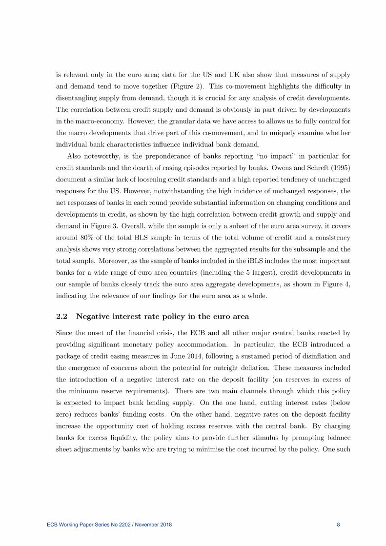
is relevant only in the euro area; data for the US and UK also show that measures of supply

and demand tend to move together (Figure 2). This co-movement highlights the difficulty in

disentangling supply from demand, though it is crucial for any analysis of credit developments.

The correlation between credit supply and demand is obviously in part driven by developments

in the macro-economy. However, the granular data we have access to allows us to fully control for

the macro developments that drive part of this co-movement, and to uniquely examine whether

individual bank characteristics influence individual bank demand.

Also noteworthy, is the preponderance of banks reporting “no impact” in particular for

credit standards and the dearth of easing episodes reported by banks. Owens and Schreft (1995)

document a similar lack of loosening credit standards and a high reported tendency of unchanged

responses for the US. However, notwithstanding the high incidence of unchanged responses, the

net responses of banks in each round provide substantial information on changing conditions and

developments in credit, as shown by the high correlation between credit growth and supply and

demand in Figure 3. Overall, while the sample is only a subset of the euro area survey, it covers

around 80% of the total BLS sample in terms of the total volume of credit and a consistency

analysis shows very strong correlations between the aggregated results for the subsample and the

total sample. Moreover, as the sample of banks included in the iBLS includes the most important

banks for a wide range of euro area countries (including the 5 largest), credit developments in

our sample of banks closely track the euro area aggregate developments, as shown in Figure 4,

indicating the relevance of our findings for the euro area as a whole.

2.2 Negative interest rate policy in the euro area

Since the onset of the financial crisis, the ECB and all other major central banks reacted by

providing significant monetary policy accommodation. In particular, the ECB introduced a

package of credit easing measures in June 2014, following a sustained period of disinflation and

the emergence of concerns about the potential for outright deflation. These measures included

the introduction of a negative interest rate on the deposit facility (on reserves in excess of

the minimum reserve requirements). There are two main channels through which this policy

is expected to impact bank lending supply. On the one hand, cutting interest rates (below

zero) reduces banks’ funding costs. On the other hand, negative rates on the deposit facility

increase the opportunity cost of holding excess reserves with the central bank. By charging

banks for excess liquidity, the policy aims to provide further stimulus by prompting balance

sheet adjustments by banks who are trying to minimise the cost incurred by the policy. One such


way that banks can reduce their cash holdings, and consequently the charge on this liquidity, is

by extending loans to the real economy (e.g., Demiralp, Eisenschmidt and Vlassopoulos (2017)).

Under this rationale, one would expect any stimulatory effects on lending to be strongest for

those banks with higher excess liquidity holdings, as their income is most explicitly impacted

by the charge.

Figure 5 shows that the deposit facility rate descended increasingly into negative territory

from the first cut of 10 basis points below zero in June 2014 to minus 40 basis points in March

2016, at which point it stabilised. The figure also shows that levels of excess liquidity were low at

the introduction of negative rates and began to increase with the introduction of the expanded

asset purchase programme in the first quarter of 2015, illustrating the important interaction

between these two policies. In the BLS, banks report directly on the effects of the negative

interest rate policy on their income, so that we can assess whether there is in fact evidence

that the lending flows at banks more exposed to the policy did in fact exhibit more positive

developments in supply.

2.3 Quantitative easing in the euro area

In January 2015, with the inflation outlook further deteriorated and with little scope for further

declines in interest rates, the ECB announced a quantitative easing policy — the expanded APP

— in order to provide further monetary policy accommodation. Since its introduction, there have

been a number of recalibrations in this programme, as shown in Figure 6. The monthly pace of

the purchases was originally set at 60bn starting in March 2015, increased to 80bn in March

2016 and decreased to 60bn in April 2017. Following the recalibration of the programme in

October 2017 the pace of monthly purchases was set to 30bn a month from January 2018

until at least September 2018. Finally, in June 2018, the Governing Council announced a

further reduction in the net asset purchases to 15 billion until the end of December 2018, at

which point purchases are expected to end. Quantitative easing can support bank credit supply

through a number of channels. Asset purchases increase bank liquidity directly through the sales

of bonds by banks and indirectly through an increase in deposits owing to their costumers’ bond

sales. As central banks purchase sovereign assets, the prices of these assets increase and their

yields decrease. Banks who sell these assets will consequently have capital gains which can ease

leverage constraints and enhance credit supply. Therefore, we would expect that banks that had

higher holdings of sovereign bonds at the start of the programme would have been more prone

to positive impulses on lending. Moreover, depressing the yields on safe assets should make


alternatives investments, such as lending to the real economy, more attractive.

Figure 7 illustrates the negative correlation between sovereign bond holdings and lending to

the non-financial private sector that is suggested in the literature on the effects of quantitative

easing. We can use the BLS information that individual banks report on the impact of the asset

purchases on their liquidity to assess whether these banks indeed saw a more positive effect on

their lending.

In the next section we formally assess the relationship between loan growth and credit supply

and demand measures (Section 3.1). Moreover, we use a financial market measure of balance

sheet constraints to assess whether, as documented for credit supply (Kashyap and Stein (2000)),

the response of demand to monetary policy shocks also differs according to bank strength (Sec-

tion 3.2). Finally, using the measure of demand as reported by banks for identification, we assess

the impact of recent unconventional monetary policy measures on loan supply (Section 3.3).

3 Empirical Evidence

This section provides empirical evidence on: i) the dependence of credit growth on demand and

supply; ii) the impact of an exogenous shock on credit demand and supply and its interaction

with bank balance sheet strength; and, iii) the impact of ECB unconventional measures on

lending growth.

3.1 Actual credit developments, and BLS supply and demand

Before proceeding with our analysis of credit supply and demand, it is necessary to ascertain

how informative these measures are for actual lending developments. To do so we estimate the

following equation:

∆ = + +

4X=1

∆− (1)

+1∆ + 2∆ +

where ∆ is the quarter-on-quarter growth rate of the total loan volume to non-

financial corporations (NFC) by bank in country in quarter . are bank fixed effects.

are country-time (in this case quarter) fixed effects.6

6Definitions and descriptive statistics of all variables used are presented in Table 1.


∆ is defined using the following question from the BLS: “Over the past

three months, how have your bank’s credit standards as applied to the approval of loans or

credit lines to enterprises changed?” The responses take a five-point scale: 1 “Tightened consid-

erably”, 2 “Tightened somewhat”, 3 “Remained unchanged”, 4 “Eased somewhat” and 5 “Eased

considerably.”

∆ is obtained using the following question from the BLS: “Over the past

three months, how has the demand for loans or credit lines to enterprises changed at your bank,

apart from normal seasonal fluctuations?” And again the responses take a five-point scale: 1

“Decreased considerably”, 2 “Decreased somewhat”, 3 “Remained unchanged”, 4 “Increased

somewhat” and 5 “Increased considerably”.

Results in Table 2 show that credit developments are jointly affected by supply and demand

pressures, not only in a statistically, but also in an economically relevant manner. The first

column in the table shows results from a panel estimation with random effects; the second column

shows the results including bank fixed effects and finally column 3 shows the results including

both bank and country-time fixed effects. Comparing the coefficients across the columns, we

can see that the inclusion of bank fixed effects diminishes the coefficient on supply substantially,

which likely indicates the importance of fixed characteristics, such as a bank’s business model,

in determining their lending strategies. On the other hand the inclusion of bank fixed effects

barely alters the coefficient on credit demand. When we saturate our model with country-time

dummies, which completely control for any variation that may be coming from macroeconomic

developments (at a country level in any time period), the coefficient on demand decreases, as

one would expect considering the importance of these factors for credit demand. However,

importantly, both supply and demand remain significant determinants of loan growth, with

similar effects over the whole period.

The coefficient of 0350∗∗ on credit supply indicates that an easing by one unit on the five-

point scale corresponds to an increase at the individual bank level of credit growth by 35 basis

points, while the coefficient of 0366∗∗ on credit demand indicates that an increase by one unit

on the five-point scale corresponds to an increase at the individual bank level of credit growth by

37 basis points.7 Trivially put, we need to account for both supply and demand when assessing

credit growth.8 This confirms the importance of the survey and its information content for loan

7As in the Tables, we indicate statistical significance as follows: *** Significant at 1%, ** significant at 5%, *

significant at 10%.8We experimented with different lag structures and found that contemporaneous credit supply and demand

have the highest explanatory power for quarter-on-quarter loan growth, which is in line with how the survey

question is phrased (i.e., it refers to changes in the most recent period).


developments.

Next, we estimate Equation (1) as a recursive regression starting with a five year window and

collate the estimates of the coefficients of bank level supply and demand in Figure 8. The results

show that the estimated coefficients on credit supply vary between 0.5 at the beginning of the

sample, which largely reflects the crisis period, and around 0.35 in the later sample period, which

includes the post-crisis period. The estimated coefficients are always statistically significant. The

coefficients on credit demand hover between 0.25 and 0.35 throughout the sample period. These

estimates suggest that actual bank credit growth and the survey measure of the bank credit

supply strongly correspond, especially during the crisis period, while with the measure of credit

demand in general there is a somewhat weaker correspondence.

3.2 Balance sheet strength, credit demand and supply

Next we estimate the impact of a monetary policy shock on credit supply and demand individ-

ually:

∆ = + +

4X=1

∆ − +−1 (2)

+Γ−1 +Θ (−1 ×−1) + Borrower +

∆ = + +

4X=1

∆ − + −1 (3)

+Λ−1 +Φ (−1 ×−1) + Borrower +

Again are bank fixed effects; are country-time dummies and −1 is the change

in the 3 month Euribor. This is similar to the monetary policy shock used in Bernanke and

Blinder (1992) and Kashyap and Stein (2000). −1 represent bank balance sheet constraints

and are the changes in individual banks’ CDS. We also include a measure of borrower risk from

the BLS, as banks are asked with regard to their borrowers how the industry or firm-specific

situation and outlook/borrower’s creditworthiness has changed.

The results in Table 3 show that banks that had increases in their CDS spread, indeed had

lower credit supply and demand, even when controlling for country time dummies. Moreover,

the interaction term in the table in columns (1) and (3), respectively, shows that a contraction


in monetary policy (increase in Euribor) will decrease both credit supply and demand more at

banks with higher CDS spreads. This indicates that in the presence of a shock, weak balance

sheets may not only alter banks’ willingness or ability to supply credit, but it may also mean

borrowers are more selective regarding their banks. This relationship also holds when controlling

in columns (2) and (4), respectively, for changes in the risk profile of the firms that borrow from

each bank. For consistency with results shown in other sub-sections, Table 3 is estimated

from mid-2007, the period for which we have both lending and survey data. Nonetheless, when

estimating equations 2 and 3 for the longer period, results are unchanged (not shown). Moreover,

Table 4 shows that the result can be replicated by interacting the monetary policy indicator with

other bank characteristics such as NPL, capital ratio and exposure to domestic sovereign bonds.

Overall these estimates on the interactive terms, especially for demand, are our key finding

and cast doubt on identification strategies that solely rely on firm(-time) fixed effects, combined

with bank characteristics, to isolate credit supply within-firm. If credit demand is also bank-

specific, which is what the estimates in Tables 3 and 4 suggest, such a strategy cannot successfully

disentangle supply from demand. Therefore, in the next section we fully account for bank-specific

credit demand when assessing the impact on lending of the ECB’s non-standard measures.

3.3 Impact of non-standard monetary policy

In this section we assess the impact on lending of the ECB’s non-standard measures, focusing

on the introduction of negative interest rates (DFR) and of the euro area’s quantitative easing

program, the so-called expanded Asset Purchase Programme (APP). We thereby effectively

account for bank-specific demand for credit.

The analysis is based on the estimation for both policy measures of a difference-in-difference

model as shown in equation (4) below. The dependent variable is the quarterly growth rate of

loans to NFC for bank in country in quarter . The model includes 4 lags of the dependent

variable. is a dummy variable equal to one for banks more impacted by the policy.

For the negative DFR, treated banks are defined as those who on average reported that the

impact of the negative interest rate policy on their net interest income was stronger.9 For the

APP, treated banks are those who on average reported that the APP impact on their liquidity

9Banks’ possible responses range from 1-5, where 3 corresponds to no impact and a lower (higher) number

indicates a stronger (weaker) impact. Since the question has been asked regularly since the introduction of the

programme, each bank’s response is averaged through time. As the median of each bank’s average response to

this question is 2, using this value as a threshold would misclassify many banks who always reported an impact

from the DFR as untreated. Therefore the threshold is set at the 75th percentile (2.5) which is closer to the

threshold of no impact (3) but still allows for an adequate control group.


position was more positive.10 is a dummy variable equal to one since the implementation

of each policy. For the negative DFR, introduced on 11 June 2014, the post period starts in

2014 Q3. For the APP, which was announced in 22 January 2015, we define the implementation

period since 2015 Q1.

Loan supply is identified by controlling for changes in demand reported by each bank in each

quarter (∆ ) and for fixed effects capturing all observable and unobservable

bank characteristics which are time invariant () as well as for all factors which are country-

specific and time-variant, i.e. for the macroeconomic environment (). The model also controls

for borrower credit risk as reported by each bank in the survey (Borrower ) and for bank

balance sheet characteristics (−1), a vector including leverage, size, amount borrowed in the

targeted long term refinancing operations (TLTROs) and liquidity). 1 is the main coefficient

of interest, showing how the behaviour of treated banks changed after the implementation of

the policy compared to untreated banks.

∆ = + +

4X=1

∆− + 1 ( × )

+3 + 2 + 4∆ (4)

+5 row +Υ−1 +

BLS banks that reported a larger impact from the negative DFR and APP tended to show

higher loan growth following the implementation of these policies (Figure 9). The figure displays

the cumulated differences in quarterly growth rates between banks in the treatment and control

groups for the negative DFR (in the left panel) and for the APP (in the right panel). As

shown in Figure 9, no systematic difference is observable in loan growth across the groups of

banks before the implementation of the measures. However, following the implementation of

the measures, banks that reported being more affected clearly increased their lending growth

by more than other banks. As already discussed, there are important interactions between the

policies, as quantitative easing injects liquidity on which the negative rates apply. Therefore,

we also analyse the consequences of being affected by both policies (relative to being affected

by neither).

10Banks’ possible responses range from 1-5, where 3 corresponds to no impact and a higher (lower) number

indicates a more positive (negative) impact. Since the question has been asked regularly since the introduction

of the programme, each bank’s response is averaged through time. The threshold is then set at 3.17 which

corresponds to the median of the distribution of each bank’s average response.


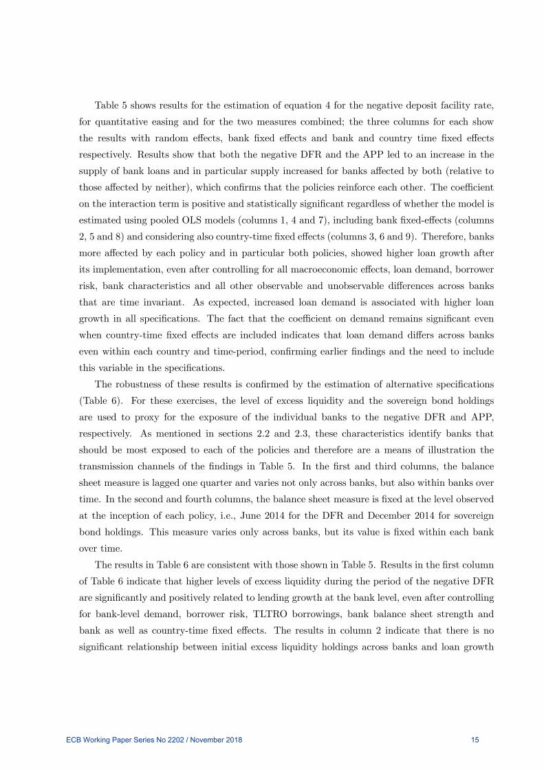
Table 5 shows results for the estimation of equation 4 for the negative deposit facility rate,

for quantitative easing and for the two measures combined; the three columns for each show

the results with random effects, bank fixed effects and bank and country time fixed effects

respectively. Results show that both the negative DFR and the APP led to an increase in the

supply of bank loans and in particular supply increased for banks affected by both (relative to

those affected by neither), which confirms that the policies reinforce each other. The coefficient

on the interaction term is positive and statistically significant regardless of whether the model is

estimated using pooled OLS models (columns 1, 4 and 7), including bank fixed-effects (columns

2, 5 and 8) and considering also country-time fixed effects (columns 3, 6 and 9). Therefore, banks

more affected by each policy and in particular both policies, showed higher loan growth after

its implementation, even after controlling for all macroeconomic effects, loan demand, borrower

risk, bank characteristics and all other observable and unobservable differences across banks

that are time invariant. As expected, increased loan demand is associated with higher loan

growth in all specifications. The fact that the coefficient on demand remains significant even

when country-time fixed effects are included indicates that loan demand differs across banks

even within each country and time-period, confirming earlier findings and the need to include

this variable in the specifications.

The robustness of these results is confirmed by the estimation of alternative specifications

(Table 6). For these exercises, the level of excess liquidity and the sovereign bond holdings

are used to proxy for the exposure of the individual banks to the negative DFR and APP,

respectively. As mentioned in sections 2.2 and 2.3, these characteristics identify banks that

should be most exposed to each of the policies and therefore are a means of illustration the

transmission channels of the findings in Table 5. In the first and third columns, the balance

sheet measure is lagged one quarter and varies not only across banks, but also within banks over

time. In the second and fourth columns, the balance sheet measure is fixed at the level observed

at the inception of each policy, i.e., June 2014 for the DFR and December 2014 for sovereign

bond holdings. This measure varies only across banks, but its value is fixed within each bank

over time.

The results in Table 6 are consistent with those shown in Table 5. Results in the first column

of Table 6 indicate that higher levels of excess liquidity during the period of the negative DFR

are significantly and positively related to lending growth at the bank level, even after controlling

for bank-level demand, borrower risk, TLTRO borrowings, bank balance sheet strength and

bank as well as country-time fixed effects. The results in column 2 indicate that there is no

significant relationship between initial excess liquidity holdings across banks and loan growth


during the negative DFR period. This result is not surprising since, as shown in Figure 5,

excess liquidity holdings were relatively low in the middle of 2014 and only began to grow in

earnest at the commencement of the quantitative easing programme in the first quarter of 2015.

Therefore, excess liquidity holdings at the initial stage would not necessarily identify banks that

were most exposed to the negative DFR over time and, in particular, those that had a large

increase in liquidity owing to the quantitative easing policy. The findings in columns 1 and 2

together underscore the important interaction between the two policies, insofar as they affected

the opportunity cost of holding excess liquidity, through prices (DFR) and quantities (APP).

The results in the second and third columns show that higher sovereign bond holdings over the

period of the APP or at the inception of the APP are associated with higher loan growth over

the course of the programme. The results in column 4 are strongest, indicating that holdings

of sovereign bonds on a bank’s balance sheet right before the central bank started to purchase

these assets most clearly identifies the banks most exposed to the policy.

4 Conclusions and macroeconomic implications

Our findings shed light on the nature of supply and demand in determining loan growth. We

show that individual banks’ supply and demand are important predictors of their lending activity

but that supply is more relevant during crisis periods. We find that demand for credit faced

by individual banks also depends on their characteristics, such as risk profile and funding.

This suggests that the assumption that firms’ credit demand tends to be randomly assorted

across banks may not always be valid, hence contributing to the important literature on the

identification and effect of credit supply shocks. Finally, we show that (effectively controlling

for loan demand) both the introduction of negative policy rates and the expanded quantitative

easing stimulated loan supply in the euro area.


References

[1] Acharya, V. V., T. Eisert, C. Eufinger, and C. W. Hirsch, 2017, Whatever it Takes: The

Real Effects of Unconventional Monetary Policy, SAFE, Frankfurt, Working Paper 152.

[2] Albertazzi, U., B. Becker, and M. Boucinha, 2018, Portfolio Rebalancing and the Trans-

mission of Large-Scale Asset Programs: Evidence from the Euro Area, European Central

Bank, Frankfurt, Working Paper 2125.

[3] Altavilla, C., M. Darracq Pariès, and G. Nicoletti, 2015, Loan Supply, Credit Markets and

the Euro Area Financial Crisis, European Cantral Bank, Frankfurt, Working Paper 1861.

[4] Altavilla, C., D. Giannone, and M. Lenza, 2016, "The Financial and Macroeconomic Effects

of the OMT Announcements," International Journal of Central Banking 12, 29-57.

[5] Arce, O., M. García-Posada, S. Mayordomo, and S. Ongena, 2018, Adapting Lending Poli-

cies When Negative Interest Rates Hit Banks’ Profits, Banco de España, Madrid, Mimeo.

[6] Berger, A. N., N. M. Miller, M. A. Petersen, R. G. Rajan, and J. C. Stein, 2005, "Does

Function Follow Organizational Form? Evidence from the Lending Practices of Large and

Small Banks," Journal of Financial Economics 76, 237-269.

[7] Berger A. N., and G. F. Udell, 2002, "Small Business Credit Availability and Relationship

Lending: The Importance of Bank Organisational Structure," Economic Journal 112, 32-53.

[8] Bernanke, B. S., and A. S. Blinder, 1992, "The Federal Funds Rate and the Channels of

Monetary Transmission," American Economic Review 82, 901-921.

[9] Billett, M.T., J. Flannery, and J.A. Garfinkel, 1995, The effect of lender identity on a

borrowing firm’s equity return, Journal of Finance 50, 699-718.

[10] Blaes, B., 2011, Bank-Related Loan Supply Factors During the Crisis: An Analysis Based

on the German Bank Lending Survey, Bundesbank, Frankfurt, Discussion Paper 31.

[11] Bowman, D., F. Cai, S. Davies, and S. Kamin, 2015, "Quantitative easing and bank lending:

Evidence from Japan," Journal of International Money and Finance 57, 15-30.

[12] Bottero Margherita, Jose-Luis Peydro, Andrea Polo, Andrea Presbitero, and Enrico Sette,

2018, "Negative Policy Rates and Bank Asset Allocations: Evidence from Italian Credit

and Security Registers", mimeo.

[13] Ciccarelli, M., A. Maddaloni, and J.-L. Peydró, 2013, "Heterogeneous Transmission Mech-

anism: Monetary Policy and Financial Fragility in the Eurozone," Economic Policy 28,

459-512.


[14] Ciccarelli, M., A. Maddaloni, and J.-L. Peydró, 2015, "Trusting the Bankers: A New Look

at the Credit Channel of Monetary Policy," Review of Economic Dynamics 18, 979-1002.

[15] Cole, R. A., L. G. Goldberg, and L. J. White, 2004, "Cookie-Cutter versus Character: The

Micro Structure of Small Business Lending by Large and Small Banks," Journal of Financial

and Quantitative Analysis 39, 227-252.

[16] de Bondt, G., A. Maddaloni, J.-L. Peydró, and S. Scopel, 2010, The Euro Area Bank

Lending Survey Matters: Empirical Evidence for Credit and Output Growth, European

Central Bank, Frankfurt, Working Paper 1160.

[17] Degryse, H., O. De Jonghe, S. Jakovljevic, K. Mulier, and G. Schepens, 2018, Identify-

ing Credit Supply Shocks with Bank-Firm Data: Methods and Applications, KU Leuven,

Leuven, Mimeo.

[18] Degryse, H. and S. Ongena, 2005, "Distance, Lending Relationships, and Competition,"

Journal of Finance, 60, 231-266.

[19] Del Giovane, P., G. Eramo, and A. Nobili, 2011, "Disentangling Demand and Supply in

Credit Developments: A Survey-Based Analysis for Italy," Journal of Banking and Finance

35, 2719-2732.

[20] Demiralp, S., J. Eisenschmidt, and T. Vlassopoulos, 2017, Negative Interest Rates, Excess

Liquidity and Bank Business Models: Banks’ Reaction to Unconventional Monetary Policy

in the Euro Area, European Central Bank, Frankfurt, Mimeo.

[21] Gambacorta, L. and P.E. Mistrulli, 2004, "Does bank capital affect lending behavior?,"

Journal of Financial Intermediation 13, 436-457.

[22] Heider, F., F. Saidi, and G. Schepens, 2017, Life Below Zero: Bank Lending Under Negative

Policy Rates European Cantral Bank, Frankfurt, Mimeo.

[23] Holmstrom, B. and J. Tirole, 1997, "Financial Intermediation, Loanable Funds, and The

Real Sector," The Quarterly Journal of Economics 112, 663-691.

[24] Jiménez, G., S. Ongena, J.-L. Peydró, and J. Saurina, 2012, "Credit Supply and Monetary

Policy: Identifying the Bank Balance-Sheet Channel with Loan Applications," American

Economic Review 102, 2301-2326.

[25] Joyce, M., and M. Spaltro, 2014, Quantitative Easing and Bank Lending: A Panel Data

Approach, Bank of England, London, Working Paper 504.

[26] Kashyap, A. K., and J. C. Stein, 2000, "What Do A Million Observations on Banks Say

About the Transmission of Monetary Policy?," American Economic Review 90, 407-428.


[27] Khwaja, A. I., and A. Mian, 2008, "Tracing the Impact of Bank Liquidity Shocks: Evidence

from an Emerging Market," American Economic Review 98, 1413-1442.

[28] Kim, Moshe, Eirik Gaard Kristiansen, and Bent Vale, 2005, Endogenous product differen-

tiation in credit markets: What do borrowers pay for?, Journal of Banking and Finance 29,

681-699.

[29] Kishan, R.P and T.P. Opiela, 2000, "Bank Size, Bank Capital, and the Bank Lending

Channel," Journal of Money, Credit and Banking 32, 121-141.

[30] Lown, C., and D. P. Morgan, 2006, "The Credit Cycle and the Business Cycle: New

Findings Using the Loan Officer Opinion Survey," Journal of Money, Credit and Banking

38, 1575-1597.

[31] Nucera, F., A. Lucas, J. Schaumburg, and B. Schwaab, 2017, Do Negative Interest Rates

Make Banks Less Safe?, European Central Bank, Frankfurt, Working Paper 2098.

[32] Owens, R. E., and S. L. Schreft, 1995, "Identifying Credit Crunches," Contemporary Eco-

nomic Policy 13, 63-77.

[33] Paravisini, D., V. Rappoport, and P. Schnabl, 2014, Comparative Advantage and Special-

ization in Bank Lending, London School of Economics, London, Mimeo.

[34] Paravisini, D., V. Rappoport, P. Schnabl, and D. Wolfenzon, 2015, "Dissecting the Effect of

Credit Supply on Trade: Evidence fromMatched Credit-Export Data," Review of Economic

Studies 82, 333-359.

[35] Petersen, M. A., and R. G. Rajan, 2002, "Does Distance Still Matter? The Information

Revolution in Small Business Lending," Journal of Finance 57, 2533-2570.

[36] Popov, A. A., and N. Van Horen, 2015, "Exporting Sovereign Stress: Evidence from Syn-

dicated Bank Lending during the Euro Area Sovereign Debt Crisis," Review of Finance 19,

1825—1866.

[37] Rajan, R.G., 1992, "Insiders and outsiders: The choice between informed and arm’s-length

debt", Journal of Finance 47, 1367—1400.

[38] Rodnyansky, A., and O. M. Darmouni, 2017, "The Effects of Quantitative Easing on Bank

Lending Behavior," Review of Financial Studies 30, 3858-3887.

[39] Schwert, M., 2018, "Bank Capital and Lending Relationships," Journal of Finance 73, 787-

830.


[40] Sharpe, S.A., 1990, "Asymmetric information, bank lending and implicit contracts: A

stylized model of customer relationships", Journal of Finance 45, 1069—1087.

[41] Stein, J. C., 2002, "Information Production and Capital Allocation: Decentralized versus

Hierarchical Firms," Journal of Finance 57, 1891-1922.


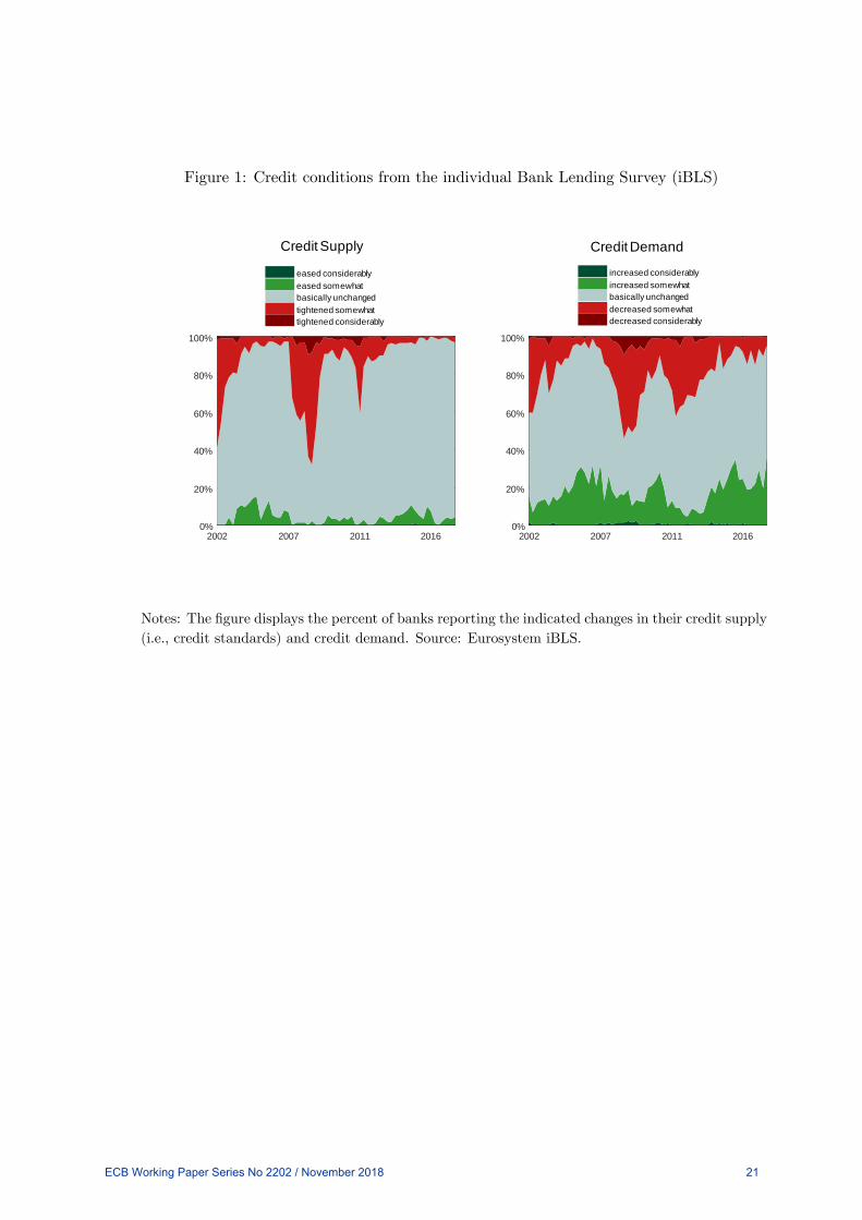
Figure 1: Credit conditions from the individual Bank Lending Survey (iBLS)

2002 2007 2011 20160%

20%

40%

60%

80%

100%

eased considerablyeased somewhatbasically unchangedtightened somewhattightened considerably

2002 2007 2011 20160%

20%

40%

60%

80%

100%

increased considerablyincreased somewhatbasically unchangeddecreased somewhatdecreased considerably

Credit Supply Credit Demand

Notes: The figure displays the percent of banks reporting the indicated changes in their credit supply

(i.e., credit standards) and credit demand. Source: Eurosystem iBLS.


Figure 2: Credit conditions across regions

2003 2008 2013 2017

-60

-40

-20

0

20

40

60

80

Euro Area

2003 2008 2013 2017

-60

-40

-20

0

20

40

60

80

UK

2003 2008 2013 2017

-60

-40

-20

0

20

40

60

80

US

Net Tightening Net Demand

Notes: Eurosystem BLS, Bank of England Credit Conditions Survey, Federal Reserve System Senior

Loan Officer Opinion Survey on Bank Lending Practices.


Figure 3: Credit standards, demand and loans to non-financial corporations

2009 2011 2013 2015 2017-60

-40

-20

0

20

40

60

80

-6

-4

-2

0

2

4

6

8

10

12

14

Total Net Tightening Total Net Demand Total NFC Loans

Notes: Net tightening is the percentage of banks reporting that credit standards tightened minus the

percentage that reported they eased. Totals calculated using country weights. Annual loan growth

calculated using iBSI data for iBLS banks. Based on the sample of banks included in iBLS.


Figure 4: Based on the sample of banks included in iBLS

2009 2011 2013 2015 2017-5

0

5

10

15

Total Euro Area iBLS Sample

Notes: The blue line shows aggregate euro area loan growth based on ECB BSI data. The red line

shows the corresponding series for the sample of banks included in the iBLS.


Figure 5: Excess liquidity and the ECB deposit facility rate

2000 2002 2004 2006 2008 2010 2012 2014 2016 2018

0

1

2

3

4

5

Policy interest ratesEoniaMRODeposit rateMarginal Lending Rate

2000 2002 2004 2006 2008 2010 2012 2014 2016 2018

0

500

1000

1500

Excess Liquidity

Notes: The figure displays aggregate excess liquidity of euro area banks (in euro billions) from

January 2000 until April 2018 and the rate on the ECB deposit facility over the same period.


Figure 6: Quantitative easing in the euro area

2015 2016 2017 20180

500

1000

1500

2000

2500

3000

3500

0

20

40

60

80

100

120

140

Pace (monthly purchases), LHS Size (cumulative purchases), RHS

Notes: The figure displays the monthly amounts of the ECB expanded asset purchase programme

and the total cumulative amounts purchased (in euro billions).


Figure 7: Government securities and lending

2010 2011 2012 2013 2014 2015 2016 2017 2018-300

-200

-100

0

100

200

300APP

Loans private sector Securities government

Notes:The figure displays the 12-month flows (in euro billions) of government securities and lending to

the private sector for euro area banks. The vertical gridline represents the date of the announcement

of the APP (January 2015).


Figure 8: Explaining loan growth with reported supply and demand

2012 2013 2014 2015 2016 2017

-0.2

0

0.2

0.4

0.6

0.8

1

2012 2013 2014 2015 2016 2017

-0.2

0

0.2

0.4

0.6

0.8

1

Recursive Coefficient 90% CI

Credit Supply Credit Demand

Notes: The figure displays the recursive estimates of the coefficients (and the corresponding 90%

confidence intervals) of a regression of the bank-level quarterly growth rate of loans to non-financial

corporation on loan supply and demand as reported by banks in the BLS for windows starting in

2007Q3 and ending in the year and quarter indicated on the x-axis (column 3 in Table 2).


Figure 9: Difference in loan growth between treated and untreated banks in the DFR and APP.

2011 2012 2013 2014 2015 2016 2017-5

0

5

10

15DFR

2013 2014 2015 2016 2017-5

0

5

10

15QE

Negative Deposit facility Quantitative Easing

Notes: The figures display the cumulated differences in quarterly growth rates between banks in

the treatment and control groups for the DFR (on the left) and APP (on the right). For the DFR,

treated banks are those who on average reported that the impact of the negative interest rate policy

on their net interest income was stronger. More specifically, the threshold is set at 2.5 in a scale of

1-5, which corresponds to the 75th percentile of the distribution of responses. For the APP, treated

banks are those who on average reported that the APP impact on their liquidity position was more

positive. More specifically, the threshold is set at 3.17 in a scale of 1-5, which corresponds to the

median of the distribution of responses.


Table 1: Growth in observed bank lending to non-financial corporations explained by bank

reported changes in credit supply and demand

Variable name Units Definition MeanStandard deviation

Bank credit variables

Loans %Quarterly growth rate of loan volume by bank b in country c in period t to non-financialcorporations

0.58 3.43

Credit supply 1-5Over the past three months, how have your bank’s credit standards as applied to the approval of loans orcredit lines to enterprises changed? 1 “Tightened considerably”, 2 “Tightened somewhat”, 3“Remained unchanged”, 4 “Eased somewhat” and 5 “Eased considerably”

2.89 0.44

Credit demand 1-5

Over the past three months, how has the demand for loans or credit lines to enterprises changed at yourbank, apart from normal seasonal fluctuations? 1 “Decreased considerably”, 2 “Decreasedsomewhat”, 3 “Remained unchanged”, 4 “Increased somewhat” and 5 “Increasedconsiderably”.

2.95 0.67

Treated APP 0-1

Dummy variable equal to 1 if a banks' average response across survey dates to thefollowing BLS question is above the median response (across all banks and dates): Overthe past six months, has the ECB's expanded asset purchase programme affected (eitherdirectly or indirectly) your bank's liquidity position? [1= considerably deteriorated; 2=somewhat deteriorated; 3=no impact; 4= somewhat improved; 5= considerablyimproved]

0.32 0.47

Treated DFR 0-1

Dummy variable equal to 1 if a banks' average response across survey dates to thefollowing BLS question is below the response at the 75th percentile (across all banks anddates): Over the past six months, how has the ECB's negative deposit facility rate, eitherdirectly or indirectly, impacted on your bank's net interest income? [1= decreasedconsiderably; 2= decreased somewhat; 3=no impact; 4= increased somewhat; 5=increased considerably]

0.73 0.45

Treated APP and DFR 0-1Dummy variable equal to 1 if Treated APP = 1 and Treated DFR = 1 and equal to 0 ifTreated APP = 0 and Treated DFR = 0.

0.55 0.50

Post APP 0-1 Dummy equal to 1 from 2015Q1 until 2017Q4 and 0 otherwise

Post DFR 0-1 Dummy equal to 1 from 2014Q3 until 2017Q4 and 0 otherwise

CDS Basis points Change in CDS spread of bank b in country c in period t 1.68 77.68

Borrower risk 1-5

Over the past three months, how have Industry or firm-specific situation andoutlook/borrower's creditworthiness affected your bank’s credit standards as applied tothe approval of loans or credit lines to enterprises? 1 "contributed considerably totightening", 2 "contributed somewhat to tightening ", 3 "Basically unchanged", 4"contributed somewhat to easing", 5 "contributed considerably to easing" of creditstandards. Inverted so that higher numbers represent higher borrower risk.

-2.82 0.50

Size Log of main assets 10.66 1.45

Liquidity RatioLiquid assets to main assets ratio. Liquid assets are defined as loans to MFIs, and debtsecurities holdings.

0.34 0.19

Leverage ratio Ratio Capital and reserves to main assets. 0.09 0.06

TLTRO % TLTRO borrowings as a share of main assets 0.60 2.02

Excess Liquidity Ratio Excess liquidity holdings as a share of main assets 0.02 0.04

Sov bond holdings Ratio Sovereign bond holdings as a share of main assets 0.06 0.06

Excess Liquidity (June 2014) Ratio Excess liquidity holdings as a share of main assets (Level fixed at June 2014 for each bank) 0.01 0.02

Sov bond holdings (Dec 2014) RatioSovereign bond holdings as a share of main assets (level fixed at December 2014 for eachbank)

0.07 0.06

Monetary policy indicator

Euribor % Change in 3-month Euribor -0.11 0.47

Notes: The table displays the variable names, units, definitions, summary statistics and data sources.

iBSI is the individual banks Balance Sheet Items Statistics from the ECB. iBLS are individual banks’

responses to the ECB Bank Lending Survery. ECB SDW is the ECB Statistical Data Warehouse.


Table 2: Growth in observed bank lending to non-financial corporations explained by bank

reported changes in credit supply and demand

Dependent variable: Loansb,c,t Loansb,c,t Loansb,c,t

Credit supplyb,c,t 0.566*** 0.305*** 0.350**(0.109) (0.110) (0.139)

Credit demandb,c,t 0.464*** 0.453*** 0.366***(0.0886) (0.105) (0.136)

Loansb,c,t-1 0.0704*** 0.0131 -0.0162(0.0243) (0.0263) (0.0341)

Loansb,c,t-2 0.159*** 0.105*** 0.0918***(0.0208) (0.0209) (0.0278)

Loansb,c,t-3 0.0767*** 0.0295 0.0479*(0.0248) (0.0263) (0.0288)

Loansb,c,t-4 0.217*** 0.175*** 0.179***

(0.0249) (0.0261) (0.0291)

Bank fixed effects No Yes YesCountry-time fixed effects No No YesNumber of observations 3308 3308 3308Number of banks 107 107 107

R2 0.153 0.201 0.360

Notes: The table displays the estimates of the coefficients in equation (1). The dependent variable

is the quarterly bank level growth rate of loans to non-financial corporations during the period

2007Q4-2017Q4. Coefficients are listed in the first row, robust standard errors that are corrected for

clustering at the bank level are reported in the row below, and the corresponding significance levels

are indicated with stars. "Yes" indicates that the set of characteristics or fixed effects is included.

"No" indicates that the set of characteristics or fixed effects is not included. *** Significant at 1%,

** significant at 5%, * significant at 10%.


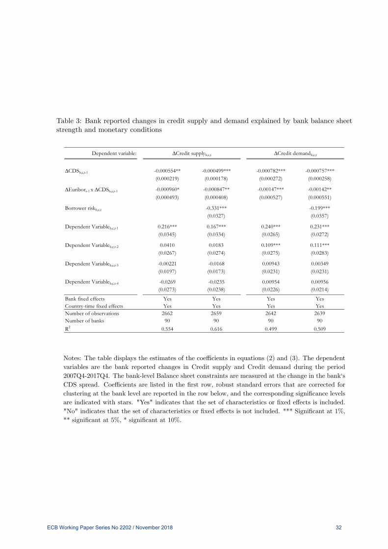
Table 3: Bank reported changes in credit supply and demand explained by bank balance sheet

strength and monetary conditions

Dependent variable:

CDSb,c,t-1 -0.000554** -0.000499*** -0.000782*** -0.000757***(0.000219) (0.000178) (0.000272) (0.000258)

Euribort-1 x CDSb,c,t-1 -0.000960* -0.000847** -0.00147*** -0.00142**

(0.000493) (0.000408) (0.000527) (0.000551)

Borrower riskb,c,t -0.331*** -0.199***(0.0327) (0.0357)

Dependent Variableb,c,t-1 0.216*** 0.167*** 0.240*** 0.231***(0.0345) (0.0334) (0.0265) (0.0272)

Dependent Variableb,c,t-2 0.0410 0.0183 0.109*** 0.111***(0.0267) (0.0274) (0.0275) (0.0283)

Dependent Variableb,c,t-3 -0.00221 -0.0168 0.00943 0.00349(0.0197) (0.0173) (0.0231) (0.0231)

Dependent Variableb,c,t-4 -0.0269 -0.0235 0.00954 0.00956(0.0273) (0.0238) (0.0226) (0.0214)

Bank fixed effects Yes Yes Yes YesCountry-time fixed effects Yes Yes Yes YesNumber of observations 2662 2659 2642 2639Number of banks 90 90 90 90

R2 0.554 0.616 0.499 0.509

Credit supplyb,c,t Credit demandb,c,t

Notes: The table displays the estimates of the coefficients in equations (2) and (3). The dependent

variables are the bank reported changes in Credit supply and Credit demand during the period

2007Q4-2017Q4. The bank-level Balance sheet constraints are measured at the change in the bank‘s

CDS spread. Coefficients are listed in the first row, robust standard errors that are corrected for

clustering at the bank level are reported in the row below, and the corresponding significance levels

are indicated with stars. "Yes" indicates that the set of characteristics or fixed effects is included.

"No" indicates that the set of characteristics or fixed effects is not included. *** Significant at 1%,

** significant at 5%, * significant at 10%.


Table 4: Bank reported changes in credit demand explained by various measures of bank balance

sheet strength and monetary conditions

Dependent variable:

Measure of Balance sheet constraint: Credit Default Swapb,c,t-1 NPLb,c,t-1 Capital Ratiob,c,t-1Domestic sovereign

holdingsb,c,t-1

Bank characteristicb,c,t-1 -0.000757*** -0.0929** -0.00431 -0.0180*(0.000258) (0.0406) (0.0127) (0.00948)

Euribort-1 * Bank characteristicb,c,t-1 -0.00142** -0.337* 0.189** -0.0369*(0.000551) (0.169) (0.0736) (0.0201)

Borrower riskb,c,t -0.199*** -0.260*** -0.239*** -0.199***(0.0357) (0.0637) (0.0620) (0.0312)

Credit demandb,c,t-1 0.231*** 0.277*** 0.203*** 0.238***

(0.0272) (0.0343) (0.0439) (0.0228)

Credit demandb,c,t-2 0.111*** 0.106** 0.1000** 0.114***(0.0283) (0.0485) (0.0402) (0.0223)

Credit demandb,c,t-3 0.00349 0.0329 -0.000108 0.0116(0.0231) (0.0682) (0.0451) (0.0231)

Credit demandb,c,t-4 0.00956 -0.0409 0.0150 0.0179

(0.0214) (0.0278) (0.0290) (0.0208)


R2 0.509 0.598 0.507 0.467

Credit demandb,c,t

Notes: The table displays the estimates of the coefficients in equation (3). The dependent variable

is the bank reported change in Credit demand during the period 2007Q4-2017Q4. Coefficients are

listed in the first row, robust standard errors that are corrected for clustering at the bank level

are reported in the row below, and the corresponding significance levels are indicated with stars.

"Yes" indicates that the set of characteristics or fixed effects is included. "No" indicates that the

set of characteristics or fixed effects is not included. *** Significant at 1%, ** significant at 5%, *

significant at 10%.


Table 5: Impact of non-standard measures on bank lending

Policy measure:

(Treatedb,c) x (Postt) 0.567*** 0.601** 0.865*** 0.561** 0.709** 0.494* 1.088*** 1.267*** 1.092**(0.215) (0.258) (0.292) (0.237) (0.280) (0.286) (0.319) (0.380) (0.426)

Postt 0.0103 0.0563 0.347* 0.440** -0.00417 0.158(0.169) (0.209) (0.177) (0.208) (0.198) (0.256)

Treatedb,c,t -0.152 -0.130 -0.303(0.160) (0.145) (0.236)

Demandb,c,t 0.401*** 0.400*** 0.358*** 0.357*** 0.334*** 0.325** 0.423*** 0.387*** 0.257(0.0984) (0.115) (0.133) (0.0971) (0.114) (0.136) (0.116) (0.120) (0.160)

Borrower riskb,c,t -0.292*** -0.112 -0.172 -0.294*** -0.134 -0.191 -0.310** -0.139 -0.196(0.0978) (0.108) (0.130) (0.0948) (0.106) (0.132) (0.153) (0.147) (0.212)

Leverageb,c,t-1 -4.537*** -6.049*** 0.352 -4.532*** -6.214** -0.272 -6.728*** -8.383* -1.905(1.038) (2.225) (3.234) (1.090) (2.450) (3.227) (2.012) (4.175) (7.024)

Sizeb,c,t-1 -0.108** -1.145*** -1.332*** -0.103** -1.170*** -1.149*** -0.132* -1.429*** -1.032(0.0425) (0.338) (0.444) (0.0438) (0.356) (0.422) (0.0675) (0.532) (0.732)

Liquidityb,c,t-1 -0.589 1.513 2.679* -0.575 1.462 2.552* -0.748 3.337** 4.355**(0.433) (1.236) (1.402) (0.450) (1.246) (1.388) (0.537) (1.443) (1.699)

TLTROb,c,t-1 0.0191 0.0392 -0.0131 -0.00504 -0.00844 -0.00307 0.0193 0.0198 0.0150(0.0180) (0.0277) (0.0389) (0.0228) (0.0336) (0.0388) (0.0312) (0.0455) (0.0534)

Dependent Variableb,c,t-1 0.0533** 0.00300 -0.0225 0.0651*** 0.0127 -0.00719 0.0303 -0.0266 -0.0287(0.0257) (0.0276) (0.0339) (0.0240) (0.0255) (0.0301) (0.0330) (0.0299) (0.0324)

Dependent Variableb,c,t-2 0.141*** 0.0945*** 0.0852*** 0.128*** 0.0800*** 0.0760*** 0.114*** 0.0588*** 0.0357(0.0220) (0.0222) (0.0274) (0.0221) (0.0224) (0.0266) (0.0255) (0.0210) (0.0305)

Dependent Variableb,c,t-3 0.0647** 0.0234 0.0437 0.0826*** 0.0408* 0.0627** 0.0526* 0.00425 0.0195(0.0254) (0.0267) (0.0289) (0.0205) (0.0215) (0.0248) (0.0291) (0.0269) (0.0352)

Dependent Variableb,c,t-4 0.211*** 0.173*** 0.176*** 0.196*** 0.157*** 0.168*** 0.199*** 0.153*** 0.140***(0.0255) (0.0267) (0.0289) (0.0257) (0.0274) (0.0293) (0.0381) (0.0410) (0.0428)

Bank fixed effects No Yes Yes No Yes Yes No Yes YesCountry-time fixed effects No No Yes No No Yes No No YesNumber of observations 3304 3304 3304 3196 3196 3196 1553 1553 1553Number of banks 106 106 106 103 103 103 49 49 49

R2 0.165 0.212 0.368 0.165 0.214 0.367 0.162 0.213 0.385

DFR APP DFR and APP

Notes: The table displays the estimates of the coefficients in equations (2) and (3). The dependent

variable is the quarterly growth rate of loans to the non-financial corporations during the period

2007Q4-2017Q4. For the DFR, treated banks are those who on average reported that the impact

of the negative interest rate policy on their net interest margin was stronger. For the APP, treated

banks are those who on average reported that the APP impact on their liquidity position was more

positive. The model includes 4 lags of the dependent variable (not shown). Robust standard errors

clustered at the bank level and reported in brackets. *** Significant at 1%, ** significant at 5%, *

significant at 10%.


Table 6: Robustness: alternative balance sheet measures to proxy for the impact of non-standard

measure

Balance sheet measure: Excess liquidity Excess liquidity (June 2014) Sovereign bond holdingsSovereign bond holdings

(December 2014)

(Balance sheet measureb,c,t-1) x (Postt) 29.58*** -13.34 5.612* 6.023**(7.773) (39.71) (3.180) (2.649)

Balance sheet measureb,c,t-1 -25.56*** -3.567(7.595) (3.560)

Demandb,c,t 0.312** 0.304** 0.352*** 0.344**(0.132) (0.134) (0.133) (0.133)

Borrower riskb,c,t -0.238 -0.193 -0.182 -0.179(0.148) (0.148) (0.131) (0.130)

Leverageb,c,t-1 0.338 0.509 -0.384 -0.128(3.486) (3.506) (3.233) (3.105)

Sizeb,c,t-1 -1.028** -1.051** -1.216*** -1.222***(0.486) (0.490) (0.455) (0.437)

Liquidityb,c,t-1 1.327 1.251 2.818* 2.586*(1.260) (1.246) (1.490) (1.405)

TLTROb,c,t-1 0.0198 0.0269 -0.0413 -0.0127

(0.0413) (0.0402) (0.0976) (0.0423)

Dependent Variableb,c,t-1 -0.0672* -0.0598* -0.0197 -0.0171(0.0351) (0.0348) (0.0326) (0.0329)


Dependent Variableb,c,t-3 0.0181 0.0225 0.0457 0.0439(0.0312) (0.0313) (0.0280) (0.0283)



R2 0.398 0.393 0.366 0.365

Notes: The Balance sheet measure used in each specification is listed at the top of the respective

column. Excess liquidity is used to proxy for the impact of the DFR; Sovereign bond holdings are

used to proxy for the effects of the APP. The dependent variable is the quarterly growth rate of loans

to the non-financial corporations during the period 2007Q4-2017Q4. Coefficients are listed in the

first row, robust standard errors that are corrected for clustering at the bank level are reported in the

row below, and the corresponding significance levels are indicated with stars. "Yes" indicates that

the set of characteristics or fixed effects is included. "No" indicates that the set of characteristics or

fixed effects is not included. *** Significant at 1%, ** significant at 5%, * significant at 10%.


Acknowledgements We would like to thank seminar participants at the ECB, the National Bank of Belgium, the 6th Workshop in Macro Banking and Finance (Alghero), De Nederlandsche Bank, 33rd Annual Congress of the European Economic Association (Cologne) for their helpful comments and suggestions. Ongena acknowledges financial support from ERC ADG 2016 - GA 740272 lending. The opinions in this paper are those of the authors and do not necessarily reflect the views of the European Central Bank or the Eurosystem.

Carlo Altavilla European Central Bank, Frankfurt am Main, Germany; email: [email protected]

Miguel Boucinha European Central Bank, Frankfurt am Main, Germany; email: [email protected]

Sarah Holton European Central Bank, Frankfurt am Main, Germany; email: [email protected]

Steven Ongena University of Zurich, Zurich, Switzerland; email: [email protected]

© European Central Bank, 2018

Postal address 60640 Frankfurt am Main, Germany Telephone +49 69 1344 0 Website www.ecb.europa.eu

All rights reserved. Any reproduction, publication and reprint in the form of a different publication, whether printed or produced electronically, in whole or in part, is permitted only with the explicit written authorisation of the ECB or the authors.

This paper can be downloaded without charge from www.ecb.europa.eu, from the Social Science Research Network electronic library or from RePEc: Research Papers in Economics. Information on all of the papers published in the ECB Working Paper Series can be found on the ECB’s website.

PDF ISBN 978-92-899-3307-0 ISSN 1725-2806 doi:10.2866/290886 QB-AR-18-082-EN-N

mailto:[email protected]




http://www.ecb.europa.eu/

http://www.ecb.europa.eu/

http://ssrn.com/

https://ideas.repec.org/s/ecb/ecbwps.html

http://www.ecb.europa.eu/pub/research/working-papers/html/index.en.html

Working Paper Series · 2018-11-20 · Working Paper Series . Credit supply and demand in...

Documents

Transcript of Working Paper Series · 2018-11-20 · Working Paper Series . Credit supply and demand in...