The Stock Market and the Corporate Sector: A Profit-Based Approach

by

Anwar M. Shaikh*

Working Paper No. 146

September 1995

*Professor of Economics, Graduate Faculty, New School for Social Research

I wish to thank Neil Buchanan for helpful comments, Robert Shiller for providing his long-term stock market data, and The Jerome Levy Economics Institute for its generous support.

Abstract

This paper shows that the empirical movements of stock prices can be explained directly by fundamentals. The real stock market rate of rctum is shown to closely track the real incremental rate of profit of the corporate sector, with the two rates displaying similar means and standard deviations. It is argued that the two are linked by capital flows between the sectors through a process we call “turbulent arbitrage”. Actual equity prices closely track the prices warranted by this model, and unlike the standard results, are less volatile than the warranted ones. The theoretical approach taken in this paper implies that the incremental profit rate is the required rate of return for the stock market rctum. The observed volatihty in stock market returns and prices arises from the fact that the required rate is itself highly volatile, driven by cyclical and other short term fluctuations in aggregate demand. It is then easy to see why conventional theoretical models, which typically assume constant required rates of return (discount rates) and constant dividend growth rates, arc largely unable to explain the movements in stock prices. On the other hand, since the incremental rate of profit (net of interest) is csscntially the change in camings normalized by investment, the findings of this paper accord well with the experience “on the street” that stock price movements are driven by intcrcst rates and changes in earnings.

1. Introduction

This paper shows that the level and volatility of the stock market rate of return can be explained directly by fundamentals -- defined here as the incremental rate of profit in the corporate sector. It is argued that the two rates are linked by the mobility of capital across sectors. This implies, among other things, that the real incremental rate of profit is the “required” rate of return for stock market.

As a general principle, higher returns in any sector tend to accelerate capital inflows into it, and lower returns tend to decelerate them. In a competitive economy, this fundamental mechanism tends to equalize (risk adjusted) rates of return across investments and sectors. Various branches of economic theory, such the theory of the firm, the law of one price, the theory of finance, and even the present value principle, depend directly on this mechanism [Dybvig and Ross 1992, p. 43; Mueller 1986, p. 8; Diermeier, Ibbotson, and Siegel 1984, p. 741.

The fact that capital can move across various applications implies that the evaluation of any given investment must always be relative to alternatives foregone in making it. This opportunity cost underlies the notion of a reference (“required”) rate of return, to which the actual return on any given investment must be compared at any moment of time, and with which it is equalized over time [Ibbotson Associates 1994, pp. 129-1301.

Under certain additional assumptions (such as constant or slowly changing required rates of return), one can derive the standard discounted present value (PV), and the dividend-discount (discounted cash flow or DCF) models of asset pricing (section 2). But these standard models do not perform well empirically (section 3). Our own approach is therefore somewhat different. We begin from the common premise that competitive risk-adjusted rates of return tend to get equalized across sectors. But instead of making the additional assumptions needed to arrive at DCF models of stock prices, we directly compare the annual stock market rate of return to the incremental rate of profit in the real sector. To this end, we develop an appropriate measure of this incremental profit rate, and show that its movements are powerfully mirrored in those of the stock market rate of return (section 4). By implication, the risk premia of the sectors are quite similar. This allows us to demonstrate that the stock market is directly driven by fundamentals, i.e. by the profits of the firms issuing stock. It also allows us to critically assess the standard DCF models.

* , 2. vfindnce theory

Much of modem finance theory is built around hypothesis that the mobility of capital equalizes risk-adjusted rates of return [Dybvig and Ross 1992, p. 48; Cohen 1987, pp. 131-1481. This includes Markowitz’s return-risk tradeoff, the approximate equality of risk-adjusted returns in

3

the Capital-Asset Pricing (CAPM) and Arbitrage Pricing Theory (APT) models, and the stochastic equality between expected and actual returns in efficient market theory’.

The present-value principle is also based on this same assumption. When applied to the stock market, this leads directly to the ubitiquous dividend-discount model, in which the price of a stock is said to be equal (in equilibrium) to the discounted present-value of the expected stream of dividends. Let r, , = the rate of return on a stock held over period t (i.e. from the beginning of period t to the beginning of period t+l), pSt = the price of the stock, d, = the dividend paid by the stock, and r, = some relevant required rare of return. Then equality of rates of return implies

1) rSt = rt , where by definition rS = *Pst+l + d,+l t

P SI

Equation 1 can be rewritten in terms of the current opening stock price.

d 2) P,, =

t+l P sl+l -+- 1 + ‘; 1 +r t

We can write a similar equation for pS ,+1 and substitute it into the right-hand side of equation 2, and then do the same thing for the remainder term involving pS t+2 , and so on. This yields

d 1+l 3) p,, = - +

4+2 P s1+2

(l+r,) U+r,>U+r,+J + (1 + rJ (1 + q+J

d t+l d =-+ I+2 d t+3 P s1+3

Cl+ q> (1+q)(l+r,+,) + (1 + rt) Cl+ q,J U+ q+2) + (1 + rJ (I+ q+J (I+ q+2>

If we assume that the remainder term approaches zero as we continue expanding the preceding

’ “The efficient market hypothesis says that the price of an asset should fully reflect all available information. The intuition behind this hypothesis is that if the price does not fully reflect all available information, then there is a profit opportunity available” which, even if small, “presumably would be attractive at large scale to many investors” [Dybvig and Ross 1992, p. 481. On the assumption that arbitrage moves to eliminate discrepancies actual prices and those expected on ‘he basis of the available information, the remaining “deviatiQns of actual returns from expected returns should be random -- they ought, on average, to be zero and uncorrelated with informaJon available to the market”[Tease 1993, p. 431.

4

expression, we are left with a familiar looking result in which the current stock price is expressed as the discounted present value of (expected) future dividends, where the discount rates are time- varying current and (expected) future required rates of return. But as Campbell notes, this restatement of the arbitrage process “is tractable only if the expected [required] returns are constant, which is one reason why the academic literature has focused for so long on this unlikely special case” [Campbell 1991, p. 1581. Imposing the strong restriction that r, = r for all t then gives us the familiar dividend-discount model of stock prices (equation 4 below). If in addition dividends are assumed to grow at some constant rate g over time , with 0 s g < r (g = 0 being the case of a constant dividend), we get the Gordon model in equation 5 below [Le Roy 1992, pp. 172-1741.

d t+k 4)p,,=C -

k-l (1 +r)k [ dividend-discount model with a constant rate of discount ]

d t+l 5) P,, = -

(r-g) ’ for r > g [ Gordon model , constant discount and dividend growth rates ]

r 3. J&e required rate of rw for the aerregate.

Equations 3-5 are merely alternate ways of expressing the assumption that over time the stock market rates of return will be kept in line with some (yet unspecified) required rate of return. For this to be meaningful, we also need a theory of the required rate itself.

Most discussions of the required rate of return begin from the assumption of perfect competition and perfect capital markets. In this case, the required rate is assumed to be “the” rate of interest, since in long run equilibrium every asset and every industry is assumed to earn a rate of return exactly equal to the interest rate. When risk (as opposed to true uncertainty) is introduced into the story, the concept of the required rate is expanded to encompass an economy-wide riskless interest rate and an asset- or industry-specific risk premium. This of course necessitates an independent means of assessing specific risk and the hypothesized risk premium associated with it, so as to construct the required rate2.

Empirical models of the aggregate stock market generally assume constant dividend growth rates and constant (or slowly varying) required rate of return, although estimates of these particular

* Various measures of risk include the familiar variance and standard deviation, as well as less familiar ones such as the mean absolute deviation, the interquartile range, and entropy. But impfAng such univariate measures into standard econotiic constructs has proved problematic. Less restricted characterizations of risk, on the other hand, only offer partial orderings of random vari:_bles [Machina and Rothschild 1987, p.202-2031.

5

rates vary substantially3. But while the resulting models are theoretically tractable, their empirical performance is quite poor [Shiller 1989, p.881. For instance, Shiller has sparked a large and growing literature with his striking demonstration of the great discrepancy between the movements of actual stock prices and those predicted by the standard dividend-discount models [Shiller 1989, p.78-821.

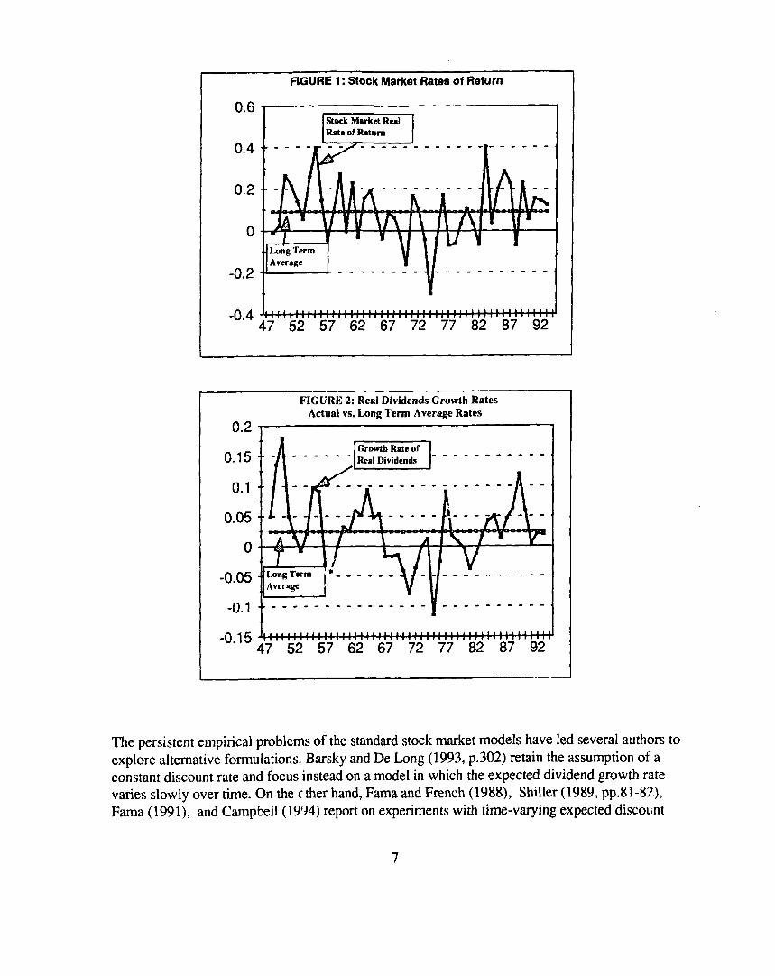
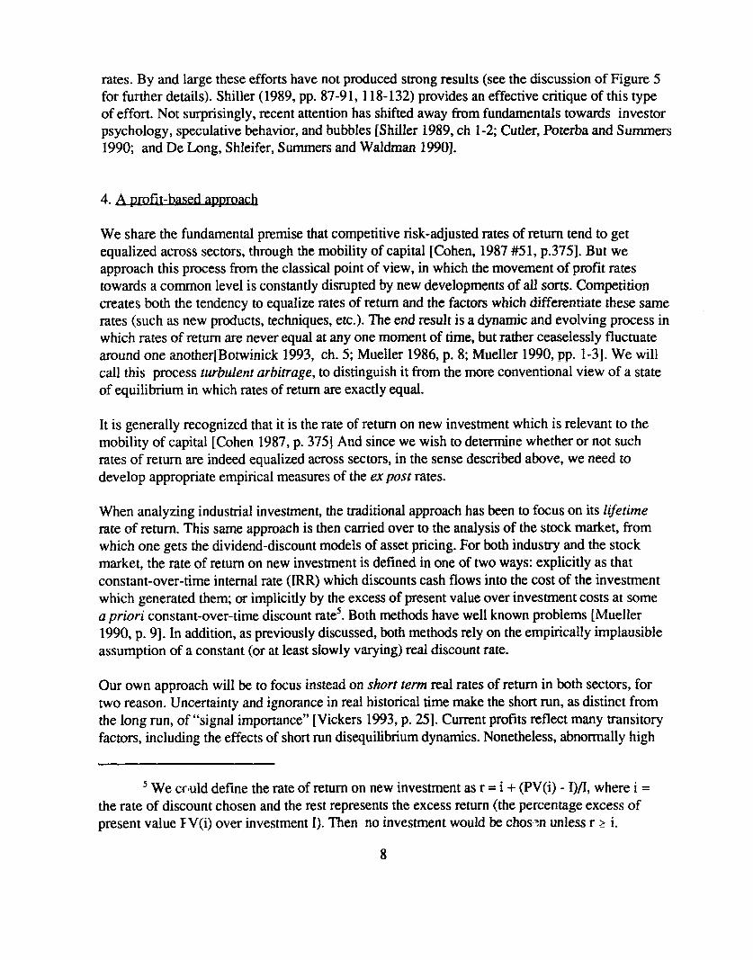
The difficulty lies in the very assumptions that make the models tractable: i.e., the hypothesized constancy of discount and dividend growth rates over time. Figures l-2 illustrate the basic problem involved. Data sources and methods are described in the Data Appendix. Figure 1 displays the actual annual rate of return in the aggregate stock market (rst ), and its long term

average (rsL LB , which can be taken to be an estimate of the corresponding required rate of retum4. It is then immediately evident that the actual real stock market rate of return exhibits great variation, as large as from -7% to +40% within the span of a year. Figure 2 depicts a similar pattern of the actual dividend growth rate. The theoretical assumption of constant expected rates of return and dividend growth rate appear particularly implausible in the face of the actual patterns. One might even say that any investor holding such expectations would have to be classified as irrational.

3 For instance, in work on the aggregate stock market, Shiller (1989, Figure 4.1, pp. 78- 79) and Ibbotson Associates (1994, pp. 136-146) estimate the discount rate from the sample mean of the real rate of return in the stock market; Barsky and De Long (1993, footnote 9 p. 300) assume a real discount rate of 6%; and Campbell uses the long term average stock market yield as the discount rate [Campbell 1991, p. 1781.

4 Shiller (1989, Figure 4.1, pp. 78-79) and Ibbotson Associates (1994, pp. 136-146) calculate the real rate of discount in this man ler.

6

flGURE 1: Stock Market Rates of Return

-0.4 llllll, llllll, 47 52 57 62 67 72 77 62 67 92

0.2

0.15

0.1

0.05

0

-0.05

-0.1

-0.15

FIGURE 2: Real Dividends Growth Rates Actual vs. Long Term Average Rates

1, ._ _. _ !k - _ _ 2

1’ I

47 52 57 62 67 72 77 82 67 92

The persistent empirical problems of the standard stock market models have led several authors to explore alternative formulations. Barsky and De Long (1993, p.302) retain the assumption of a constant discount rate and focus instead on a model in which the expected dividend growth rate varies slowly over time. On the c ther hand, Fama and French (1988), Shiller (1989, pp.81-8?), Fama (1991), and Campbell (1904) report on experiments with time-varying expected discount

rates. By and large these efforts have not produced strong results (see the discussion of Figure 5 for further details). Shiller (1989, pp. 87-91, 118-132) provides an effective critique of this type of effort. Not surprisingly, recent attention has shifted away from fundamentals towards investor psychology, speculative behavior, and bubbles [Shiller 1989, ch l-2; Cutler, Poterba and Summers 1990; and De Long, S hleifer, Summers and Waldman 19901.

We share the fundamental premise that competitive risk-adjusted rates of return tend to get equalized across sectors, through the mobility of capital [Cohen, 1987 #51, p.3751. But we approach this process from the classical point of view, in which the movement of profit rates towards a common level is constantly disrupted by new developments of all sorts. Competition creates both the tendency to equalize rates of return and the factors which differentiate these same rates (such as new products, techniques, etc.). The end result is a dynamic and evolving process in which rates of return are never equal at any one moment of time, but rather ceaselessly fluctuate around one another[Botwinick 1993, ch. 5; Mueller 1986, p. 8; Mueller 1990, pp. l-31. We will call this process turbulent arbitrage, to distinguish it from the more conventional view of a state of equilibrium in which rates of return are exactly equal.

It is generally recognized that it is the rate of return on new investment which is relevant to the mobility of capital [Cohen 1987, p. 3751 And since we wish to determine whether or not such rates of return are indeed equalized across sectors, in the sense described above, we need to develop appropriate empirical measures of the ex past rates.

When analyzing industrial investment, the traditional approach has been to focus on its lifetime rate of return. This same approach is then carried over to the analysis of the stock market, from which one gets the dividend-discount models of asset pricing. For both industry and the stock market, the rate of return on new investment is defined in one of two ways: explicitly as that constant-over-time internal rate (IRR) which discounts cash flows into the cost of the investment which generated them; or implicitly by the excess of present value over investment costs at some a priori constant-over-time discount rate’. Both methods have well known problems ]Mueller 1990, p. 91. In addition, as previously discussed, both methods rely on the empirically implausible assumption of a constant (or at least slowly varying) real discount rate.

Our own approach will be to focus instead on short term real rates of return in both sectors, for two reason. Uncertainty and ignorance in real historical time make the short run, as distinct from the long run, of “signal importance” [Vickers 1993, p. 251. Current profits reflect many transitory factors, including the effects of short run disequilibrium dynamics. Nonetheless, abnormally high

’ We cctuld define the rate of return on new investment as r = i + (PV(i) - I)& where i = the rate of discount chosen and the rest represents the excess return (the percentage excess of present value FV(i) over investment I). Then no investment would be chosen unless r 2 i.

8

or low profits alter capital flows, which in turn brings “new uncertainties and new positions of profits and loss”, which feedback on capital flows, and so on. What obtains is a series of ceaseless fluctuations in which current profits play a central role [Geroski and Mueller, 1990, p. 187; Mueller 1986, p.81.

There is also the fact that stock market investment is, by its very nature, inherently short term. Unlike their industrial counterparts, stock market investors have very little in the way of sunk costs or transaction costs. The stock market rate of return is therefore a highly contingent one. Insofar as it is compared to the rate of return in other sectors, the comparison is likely to be to very current measures of return, not to long term ones.

Both of the preceding arguments suggest that the required rate of return for the financial markets lies in the real sector. But this implies that financial capital regulates the stock market. But how is this possible, given that individual investors play so large a role in the stock market? The answer is that it is only necessary for financial capital to add or subtract sujj’icient investments in the stock market so as to regulate its rate of return, over some relevant time scale. This does not exclude the possibility of fads and fashions. Rather, it affirms the fact that in the end fundamentals do rule [Shiller 1989, pp.374-3761.

The current rate of return in the stock market was defined previously in equation 1. If the relevant variables are expressed in real terms, then it is a real rate. What remain, therefore, is to define a corresponding short-term rate of return in the corporate sector. At any moment of time, the current profits P, earned by a firm are the sum of the current profits on the most recent investment (rt I, .,) and the current profits on all earlier vintages (P’, ). The latter term represent the current profit that would have accrued in the absence of investment I,_,. From this, we can write

6) AP, = P,-P,_, = r,I,_, + (P/-P,_,)

The shorter the evaluation horizon, the closer will be current profit on carried-over vintages (P’, ) to last period’s profit on the same capital goods (P,.l). We will assume that for relevant short- term horizon (up to a year) that the difference between these two is negligible. Then the current rate of return on new investment [Elton and Gruber 1991, p. 4541 is simply

Apt 7) rt = - ( i I t-1

If real profits P, and investment I,_, are net magnitudes, then r, is the (net) incremental rate of return on capital (since net investment = AK,_, , where K, is the real capital stock at the beginning of the period t). When profits and investment are in gross terms, we may think of r, as either the gross incremental rate of return, or as an approximation to the net rate. This is a matter of some empiecal significance, because net rates require adequate measure? of depreciation and retirement investment, and their are many well-known problems associated estimates of these magnitudes

9

peldstein and Rothschild 1974; Usher 19801.

In comparing stock market and corporate profitability, it is important to recognize that corporate profits are shown net of all interest payments. We therefore use the stock market net (of interest) rate of return, rlSI = r,, - i, , where i, = the real prime rate of interest charged by banks (see the Data Appendix for further details)6. Figure 3 compares the current real net stock market rate of return rtS, , to the (gross of depreciation but net of interest) accounting rate of return R, = P,/K, often used as a proxy for the long term rate of return [Mueller 1990, p.91, while Figure 4 compares rlS t to the real gross incremental corporate rate of return r, . It is immediately apparent that the average rate R, performs very poorly in explaining the stock market rate of return. The the real incremental rate r, , on the other hand, performs extremely well indeed. The correlation between the former two is only 0.048, while that between the latter two is 0.414.

FIGURE 3: Rates of Return Stock Market & Avg Corporate Rate

47 52 57 62 67 72 77 62 87 92

6 The net interest component of corporate income excludes corporate interest payments to the financial sector. One could try to estimate these and add them back into total profits, but the relevant data from the Internal Revenue Stati.:tics of Income appears only after a three-year lag.

10

FIGURE 4: Rates of Return Stock Market & Incremental Corp Rate

-0.4 - 47 52 57 62 67 72 77 82 87 92

The concept of turbulent arbitrage proposed in this paper does not require a close correlation between two variables. It would be possible, for instance, to have two variables fluctuate around each other and yet not be statistically correlated7. But they would have to be “close” in some sense, such as in the mean, or perhaps in terms of percentage mean absolute or squared deviations. In our case, the close visual correspondence between the two rates of return depicted in Figure 4 is well reflected in the similarity of their means, standard deviations, and coefficients of variation (standard deviation/mean), as shown in Table 1.

Table 1: Comparative Statistics for Stock Market and Corporate Real Returns

Mean Standard Deviation Coeff. of Variation

S&P 500 Net Rate of 0.0603 0.1361 2.2570 Return (rs, - i, )

Return on New Corp. 0.0678 0.1463 2.1578 Investment (AP, /It _, )

7 A simple case is of two (sa;r) rates of return rZ1 = r, t + E, where E = a small random variable with zero mean, and r, L = a constant. Then r, , and rZt are close to one another, fluctuate around each other, have tht same means, but are completely uncorrelated.

11

A central puzzle in the stock market literature concerns the “unexplained volatility” of equity prices relative to those predicted by standard models [Shiller 1989, p. 79; Tease 1993, p.421. But we have seen that these models are predicated on the empirically unsupportable assumptions of

_ constant discount rates an’d dividend growth rates. Our own approach shows that the stock market rate of return (net of interest) closely parallels the current return on new corporate investment. Since the latter is essentially a normalized measure of the change in earnings (net of interest), this finding strongly supports the well known concern of stock market investors with interest rates and changes in earning?. It also confirms the general sense that “investors should not expect a much greater or fear a much smaller rate of return than that provided by businesses in the real economy” [Diermeier, J.J., Ibbotson, R. G., and Siegel, L. B. 19841.

The preceding findings sheds new light on the volatility problem. Given the relative smoothness of dividends per share, it is precisely the volatility of stock prices which enables the stock return to track the underlying fundamentals. Indeed, it is now the volatility of the fundamentals themselves, i.e. of the incremental rate of profit, which becomes the issue. And here, we find that it is short termfluctuations in aggregate demand, as expressed in the capacity utilization rate, which accounts for the volatility of the incremental profit rate’.

But might this volatility still be too great? The question can be tackled directly by comparing actual equity prices to those warranted by our model. We have only argued that turbulent arbitrage makes the net stock market rate of return rlSt = rSt - i, (where i, = the real rate of interest) roughly equal to the current return on new corporate investment r, . But we can ask what equity prices would make them exactly equal. In this case equation 1 holds exactly, and we get

8) P,; = P, L _, 1 + (rt+ - [ y, , )] = the real warranted equity price

where r: = r, + i, = the incremental corporate return inclusive of interest opportunity cost,

and Yst =dt/Ps,-1 = the equity yield. Figure 5 compares the estimated real warranted equity

price PSI” to the actually observed real equity price ps , . Following Shiller, both of them are den-ended by dividing them by a 30-year moving average of real earnings per share. This makes them comparable to his famous diagrams [Shiller 1989, pp. 78-821.

* Peavy argues that “variations in stock prices can largely be explained by changes in the cash flow [gross profits] of corporations and changes in the discount rate that prices these cash flows... [which is why] investors carefully monitor movements in corporate profits and interest rates” [Peavy 1992, p. lo].

9 Although we cannot pursue it here, it is possible to show that changes in corporate real investment can b: linked to changes in real profits, and that the sharp fluctuatkons in the latter reflect changes in capacity utilization.

12

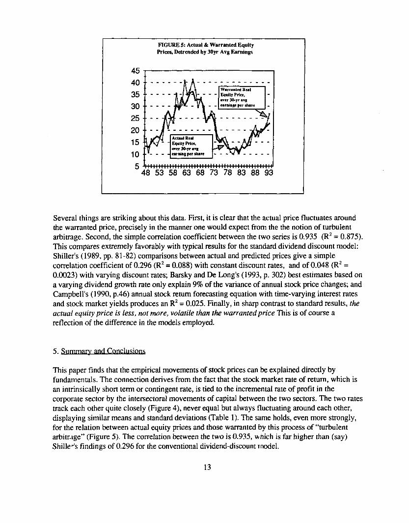
FIGURE 5: Actual & Warranted Equity

Prices, Detrended by 30yr Avg Earnings

. . _ _ _ _ - _ -_-_---_-____

Wsrrmkd Real -- _ _ - _ Equity Price, a- wcr 30-p l *p,

cmblnp per share _ .:. -_-_____ d -_-___

x5 --Au---

4% 53 58 63 68 73 78 83 88 93

Several things are striking about this data. First, it is clear that the actual price fluctuates around the warranted price, precisely in the manner one would expect from the the notion of turbulent arbitrage. Second, the simple correlation coefficient between the two series is 0.935 (R2 = 0.875). This compares extremely favorably with typical results for the standard dividend discount model: Shiller’s (1989, pp. 81-82) comparisons between actual and predicted prices give a simple correlation coefficient of 0.296 (R2 = 0.088) with constant discount rates, and of 0.048 (R* = 0.0023) with varying discount rates; Bat-sky and De Long’s (1993, p. 302) best estimates based on a varying dividend growth rate only explain 9% of the variance of annual stock price changes; and Campbell’s (1990, p.46) annual stock return forecasting equation with time-varying interest rates and stock market yields produces an R2 = 0.025. Finally, in sharp contrast to standard results, the actual equity price is less, not more, volatile than the warranted price This is of course a reflection of the difference in the models employed

This paper finds that the empirical movements of stock prices can be explained directly by fundamentals. The connection derives from the fact that the stock market rate of return, which is an intrinsically short term or contingent rate, is tied to the incremental rate of profit in the corporate sector by the intersectoral movements of capital between the two sectors. The two rates track each other quite closely (Figure 4), never equal but always fluctuating around each other, displaying similar means and standard deviations (Table 1). The same holds, even more strongly, for the relation between actual equity prices and those warranted by this process of “turbulent arbitr,ige” (Figure 5). The correlation between the two is 0.935, which is far higher than (say) ShilleQ findings of 0.296 for the conventional dividend-discount model.

13

The theoretical approach taken in this paper implies that the incremental profit rate (which is net

of interes r G AP,,,, + 4+1

St t) is the required rate of return for the stock market return (net

P qr

of interest). Since this required rate is highly volatile, itself driven by short term fluctuations in aggregate demand, the volatility in returns (Figure 4) and stock prices (Figure 5) is thereby explained by movements in the real sector. It is then easy to see why conventional theoretical models, which typically assume constant required rates of return (discount rates) and constant dividend growth rates, are largely unable to explain the movements in stock prices. On the other hand, since the incremental rate of profit is the change in earnings normalized by investment, the findings of this paper accord well with the experience “on the street” that stock price movements are driven by interest rates and changes in earnings.

The stock market data refers to the S & P 500 index of common stocks [Standard and Poors 1993, and earlier data]. Nominal dividends per share d’ were derived by multiplying the current yield (d’/p: ) by the nominal stock price index p15 . Both were deflated by the implicit price deflator for total gross private domestic fixed investment (1987=100) as shown in the Economic Report of the President [ERP1995, Table B-31 and then used to calculate the real stock market rate of return r,, (equation 1 and Figure 1) and the growth rate of real,dividends (Figure 2). Finally, the real rate of interest it was calculated as the difference between the nominal prime rate of interest charged by banks [ERP1995, Table B-721 and the rate of growth of the investment deflator described above, and this was used to calculate the net stock market rate of return r: t = r, t - it (Figures 3-4). Average real earnings used to detrend the price series (Figure 5) was constructed from data on long term earnings per share and on producer prices (1982=100) generously provided by Robert Shiller.

The corporate data refers to the domestic U.S. economy. The beginning-of-year capital stock K L

is for total (nonresidential and residential) fixed private corporate capital, gross stock, end-of- year, constant-cost valuation, in million of 1987 dollars, shifted forward one year [BEA 1993, Tables A6, A9, and subsequent updates]. Real investment I,, in 87-$, is the sum of fixed private corporate nonresidential and residential investment [BEA 1993, Tables B4, B6, and subsequent updates]. Real corporate profits P, were calculated by deflating nominal total domestic (corporate) profits, gross of capital consumption allowances, by the investment deflator. The former was calculated as the sum of nonfinancial and financial profits, lines 3+4, Tables 6.16 A- C, National Income and Product Accounts[BEA 1992-93, and subsequent updates] and corporate consumption of fixed capital ( ibid, Table 8.11, line 2). The average real rate of profit (Figure 3) was calculated as P, /Kt , and the incremental rate of profit (Figure 4) as rt = AP, /It _i .

14

Barsky, R. B. and J. B. De Long (1993). “Why Does the Stock Market Fluctuate?” QuarterZy Journal of Economics CVIII(2): 29 1.

BEA (1992-93). National Income and Product Accounts, 2 Vols. Washington, D.C., Bureau of Economic Analysis.

Botwinick, H. (1993). Persistent Inequalities: Wage Disparities under Capitalist Competition. Princeton, N.J., Princeton University Press.

Campbell, J. (1991). “A Variance Decomposition for Stock Returns.” The Economic Journal 101 (March): 157.

Campbell, J. Y. (1990). “Measuring the Persistence of Expected Returns.” AEA Papers and Proceedings 80(2): 43.

Cohen, J. B., E. D. Zinbarg, et al. (1987). Investment Analysis and Portfolio Management. Homewood, III., Irwin.

Cutler, D. M., J.M. Poterba and L.H. Summers (1990). “Speculative Dynamics and the Role of Feedback Traders.” NBER Working Paper No. 2385.

De Long, J. B., Andrei Shleifer, Lawrence H. Summmers, and Robert J. Waldman (1990). “Noise Trader Risk and Financial Markets.” Journal of Political Economy 98(4): 703.

Diermeier, J. J., R.G. Ibbotson and L.B. Siegel (1984). “The Supply of Capital Market Returns.” Financial Analysts Journal (March-April); 74.

Dybvig, P. H. and S. A. Ross (1992). “arbitrage.” The New Palgrave Dictionary of Money and Finance 1: 43.

Elton, E. J. and M. J. Gruber (1991). Modern Por@olio Theory and Investment Analysis. New York, John Wiley & Sons, Inc.

ERP (1995). Economic Report of the President. Washington, D.C., U.S. Govt. Printing Office.

Fama, E. F. (1991). “Efficient Capital Markets: II.” Journal of Finance S(December).

Fama, E. F. and K. R. French (1988). “Permanent and Temporary Components of Stock Prices.” Journal of Political Economy 92(2): 246.

15

Feldstein, M. S. and M. Rothschild (1974). “Towards an Economic Theory of Replacement Investment.” Econometrica 42(3).

Ibbotson, R. and a. Associates (1994). Stocks, Bonds, and Inflation: 1994 Yearbook. Chicago, Ibbotson Associates.

Le Roy, S. F. (1992). “stock prices and martingales.” The New Palgrave Dictionary of Money and Finance 3: 588.

Machina, M. J. and M. Rothschild (1992). “risk.” The New Palgrave Dictionary of Money and Finance 3: 201.

Mueller, D. C. (1986). Profits in the Zong run. Cambridge, Cambridge University Press.

Mueller, D. C., Ed. (1990). The dynamics of company profits: an international comparison. Cambridge, Cambridge University Press.

Peavy, J. W. (1992). “Stock Prices: Do Interest Rates and Earnings Really Matter?” Financial Analysts Journal (6): 10.

Shiller, R. J. (1989). “Comovements in Stock Prices and Comovements in Dividends.” The Journal of Finance 44(3): 7 19.

Standard and Poors (1993). Standard and Poors Analysts Handbook: OfJicial Series. New York.

Tease, W. (1993). “The Stock Market and Investment.” OECD Economic Studies No. 20(Spring): 41.

Usher, D., Ed. (1980). The Measurement of Capital. Studies in Income and Wealth. Chicago, University of Chicago Press.

Vickers, D. (1993). “The investment function: five proposition& response to Professor Gordon.” Can the Free Market Pick Winners? What Determines Investment. At-monk, New York, M.E. Sharpe. 23.

16