Working Paper - humcap.uchicago.eduhumcap.uchicago.edu/RePEc/hka/wpaper/Golsteyn_Hirsch_2018... ·...
51
HCEO WORKING PAPER SERIES Working Paper The University of Chicago 1126 E. 59th Street Box 107 Chicago IL 60637 www.hceconomics.org
Transcript of Working Paper - humcap.uchicago.eduhumcap.uchicago.edu/RePEc/hka/wpaper/Golsteyn_Hirsch_2018... ·...

HCEO WORKING PAPER SERIES
Working Paper
The University of Chicago1126 E. 59th Street Box 107
Chicago IL 60637
www.hceconomics.org

1
Are estimates of intergenerational mobility biased by
non-response? Evidence from the Netherlands*
Bart H. H. Golsteyn, Stefa Hirsch
Abstract: Intergenerational mobility is often studied using survey data. In such settings, selective unit
or item non-response may bias estimates. Linking Dutch survey data to administrative income data
allows us to examine whether selective responses bias the estimated relationship between parental
income and children’s mathematics and language test scores in grades 6 and 9. We find that the
estimates of these relationships are biased downward due to parental unit non-response, while they are
biased upwards due to item non-response. In the analyses of both unit and item non-response, the point
estimates for language and mathematics test scores point in the same direction but only one of the two
relationships is significant. These findings suggest that estimates of intergenerational mobility based
on survey data need to be interpreted with caution because they may be biased by selective non-
response. The direction of such bias is difficult to predict a priori. Bias due to unit and item non-
response may work in opposing directions and may differ across outcomes.
Keywords: intergenerational mobility, unit non-response, item non-response
JEL: I24, J62
* This project is partly financed by a VIDI grant from the Netherlands Organization for Scientific Research
(NWO) as well as grants from the Network of Social Innovation (Maastricht University) and the Dutch Ministry
of Education, Culture and Science. Data collection was funded by the Dutch Ministry of Education as well as by
the school boards in the province of Limburg. We thank the editor, two anonymous referees, Paul Jungbluth,
Tyas Prevoo, Trudie Schils, Lex Borghans, and Roxanne Korthals for their useful feedback. Furthermore, we
thank conference participants at the Dutch Economists’ Day 2015, the 21st meeting of the Society of Labor
Economists (2016), the 30th conference of the European Society for Population Economics (2016), and the 28 th
meeting of the European Association of Labour Economists, as well as seminar participants at Maastricht
University and Tübingen University for their helpful comments. Department of Economics, Maastricht University, P.O. Box 616, 6200 MD, Maastricht, the Netherlands.
Phone: +31 43 388 3736. [email protected]. Department of Economics, Maastricht University, P.O. Box 616, 6200 MD, Maastricht, the Netherlands.
2
1 Introduction
The relationship between parental income and children’s schooling outcomes is often estimated using
survey data (see, e.g., Blau 1999; Chevalier, Harmon, O’Sullivan & Walker 2013; Plug & Vijverberg
2005).1 A potentially important issue in the literature on intergenerational mobility is that survey
response is potentially not random. Most notably, the probability of responding to a survey has been
shown to be positively related to income and other indicators of socio-economic status (see the
literature review below). An unresolved question is whether non-response biases the estimated
intergenerational relationship between parental income and child schooling.
In this study, we examine whether survey-based estimates of the relationship between
household income and children’s performance in school are biased because of selective non-response.
We focus on two sources of non-response: (1) individual unit non-response by parents unwilling to
participate in a survey, and (2) item non-response by parents on questions regarding their income.
We combine parental survey data with administrative data from schools and income register
data. Our analysis is based on an ongoing regional education survey conducted in the south of the
Netherlands covering more than 95 percent of primary schools in the target region. Parental survey
information is available for approximately 69 percent of children. We link the data relating to the
children to the administrative income data of their parents, which are drawn from Statistics
Netherlands. This source provides us with information on parental income for those who respond and
do not respond to the survey. Our variable of interest – children’s school performance on standardized
mathematics and language tests in grade 6 and 9 – is based on the schools’ administrative records.
All our estimations are performed using administrative data only, from schools as well as the
income register. We distinguish different types of non-response biases by using observed survey
response behavior to artificially restrict the full sample to the data that would be available had the
survey suffered from a certain type of non-response.2 Observing non-responding households using
1 Other studies use administrative data (see, e.g., Black, Devereux & Salvanes 2005). Black and Devereux
(2011) provide an extensive review of this literature and the different empirical methods used. 2 Similar approaches to comparing survey data with full population register data have been taken in health
science (Reijneveld & Stronks 1999; Søgaard, Selmer, Bjertness & Thelle 2004) and by Micklewright and
Schnepf (2006) to assess response bias in the PISA study in the UK.
3
administrative information enables us to directly assess whether response rates are selective and
whether the relationship between parental income and child school performance is biased.
Our main findings are, firstly, that unit non-response at the household level attenuates the
intergenerational relationship. Secondly, we find evidence that item non-response on the income
question leads to an overestimation of the relationship between parental income and children’s test
scores. In the analyses of both unit and item non-response, the point estimates for language and
mathematics test scores point in the same direction, but only one of the two relationships is significant.
This study contributes to the literature on intergenerational mobility, specifically the empirical
literature that analyzes how children’s schooling outcomes relate to parental income.3 Cross-sectional
surveys find a consistently significant positive relationship between parental income and schooling
outcomes (Blau 1999; Chevalier et al. 2013). Also, when adoption is used as a natural experiment to
exclude genetically transferred ability as a factor, the significant relationship with income persists
(Plug & Vijverberg 2005). This result remains robust when controlling for characteristics of biological
parents and extend the focus to the economic outcomes of the children (Björklund, Lindahl & Plug
2006). Hence, parental income appears to be an important determinant of success in school and the
labor market.
While findings on the direction of the relationship between parental income and children’s
outcomes are unambiguous, their magnitude is often contested. There are several potential empirical
problems in studies based on survey data: e.g., non-representative samples, truncated samples, survey
non-response, and item-based non-response. Many samples are non-representative by construction, but
truncations could also be the result of a choice, such as excluding observations with low or no income.
The latter likely leads to overestimations of intergenerational correlations (Couch & Lillard 1998).
Unit non-response is inevitable and ubiquitous in survey studies: virtually all self-reported measures of
income are subject to item-based non-response.4 The question, both with respect to unit and item non-
3 Educational performance is an important predictor of later labor market outcomes (Murphy & Peltzman 2004).
Education in general is considered an important mechanism to transmit power from one generation to the next
(Wolff 2016). 4 Riphahn and Serfling (2005) explore this phenomenon and relate it to several demographic and interviewer
characteristics. As Bielby, Hauser, and Featherman (1977) show, response errors may lead to overestimations of
the racial gap and in turn to other severe misinterpretations.

4
response, is whether the non-response is selective and if so how this may bias the estimated
intergenerational relationship.
Earlier research has shown that unit and item non-response are selective in the sense that they
are related to income. According to the literature on social‐desirability bias, income is a sensitive topic
that many survey respondents do not want to speak about. Tourangeau & Tang (2007) show, for
instance, that item non-response on income questions is higher than on questions related to sexuality.
Bollinger & Hirsch (2013) report that item non-response is higher on income questions than on other
questions in the Current Population Survey. Lillard, Smith & Welsh (1986) show that non-response
across the earnings distribution is U-shaped, i.e., that respondents in the tails are least likely to report
earnings.5 These findings are confirmed by, among others, Bollinger et al. (2017) and Bee et al.
(2016), who compare survey responses with administrative data.6 A valuable point to mention here is
that administrative data do not necessarily provide true information on income, as they could, e.g., fail
to account for undeclared income. 7
While there is ample evidence that unit and item non-response are related to income, the issue
of whether selective non-response biases estimates of intergenerational mobility has, to our
knowledge, not yet received attention in the literature. The contribution of our study is to identify and
assess the magnitude of unit and item non-response bias in the context of the intergenerational
relationship between parental income and children’s schooling.
The remainder of the study is structured as follows. Section 2 provides a description of the
data. Section 3 covers the empirical approach. Section 4 discusses the results. Section 5 highlights
potential mechanisms and Section 6 concludes.
5 Some studies have imputed missing responses based on geographically-aggregated data (e.g., Sabelhaus et al.
2015). Since Lillard, Smith & Welsh (1986) (for recent evidence see, e.g., Bee, Gathright & Meyer 2016),
questions regarding the validity of this approach have been raised. 6 For more evidence that survey response is positively related to income see, e.g., Martikainen, Laaksonen, Piha
& Lallukka 2007, Porter & Whitcomb 2005, or Turrell, Patterson, Oldenburg, Gould & Roy 2003. 7 Although misreporting of income is not the main focus of our analysis, our results do relate to this issue as
well. Research on measurement error regarding earnings has linked survey data to administrative record data
(see, e.g., the survey by Bound et al. 2001). One of our analyses compares the correlation between the
administrative measure of income and educational outcomes with the correlation between a self-reported
measure of income and educational outcomes. The results show that the latter is attenuated relative to the former.
This is in line with the analysis by Hariri & Lassen (2017) who show that high-income earners tend to overstate
their income. Similar to our analysis, they also compare administrative measures of income with self-reported
measures. The context of their study differs from ours, however, in the sense that they study the relationship
between income and political attitude.

5
2 Data
We combine different sources of administrative records and survey data. The basis of our dataset is an
ongoing regional education monitor for the south of the Netherlands: the OnderwijsMonitor Limburg
(OML). The monitor has been conducted as a cooperative project between schools and Maastricht
University since 2009. Almost all primary schools in the southern part of the Dutch province of
Limburg participate in the project and provide records on their students on a yearly basis.8
The data we use are gathered for one cohort of students at two points in time. The students
were observed in 2009 in grade 6 (their last year of primary school, completed on average at age 12)
and in their third year of secondary school in grade 9 (at about age 15). We give more information
about the data below.
At both points in time, a parental survey was conducted and the results linked to the school
records. For grade 6, the parental survey was distributed via the school. In grade 9, the survey was
distributed directly to the parents. For the grade 6 data, the overall response rate among the parents
amounted to 69 percent.9 Approximately one third of all non-responding parents had children studying
in schools in which none of the parents participated in the survey. This makes it highly likely that
those schools either did not send out the survey to the parents or did not forward the completed
questionnaires back to the university. In the following, these schools will be referred to as “non-
responding schools” so as not to confuse them with schools not participating in the OML. Therefore,
in our analysis we distinguish non-response at the parental level (22 percent) and non-response at the
institutional or school level (9 percent). Since non-response at the institutional level is idiosyncratic to
our survey design, we discuss the results on this type of non-response in the appendix. We do provide
the main descriptive statistics of this type of non-response in the main text, however.
8 Additional information about the monitor can be found in the appendix. 9 This compares very well to the response rates or survival rates in the articles by Chevalier et al. (2013) and by
Plug and Vijverberg (2005), as can be seen from technical reports on the underlying surveys (EUROSTAT 2009;
Hauser 2005). The response rate of 58 percent reported by Björklund et al. (2006) is somewhat lower. The only
higher response rate in any of the articles on the estimated relationship between parental income and child
schooling cited above amounts to 87 percent in the National Longitudinal Survey of Youth (NLSY) used by
Blau (1999).

6
In the grade 9 survey, the overall parental response rate of 43 percent is substantially lower
than in the survey conducted in grade 6, even though the parental survey was distributed directly to the
parents.10 The surveys also differ in content. In grade 9, a question regarding household income was
included in the parental survey, allowing us to additionally analyze the effect of item non-response on
the income questions. Approximately 63 percent of the responding parents did not fill out the income
question.
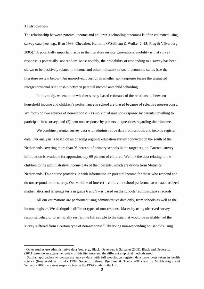
The process of data collection, as well as the approximate response and non-response rates for
both samples, are depicted in Figure 1. Parental unit non-response can be observed in both samples.
Institutional unit non-response can only be assessed in the grade 6 sample and item non-response only
in the grade 9 sample.
We merge the data from this cohort to the administrative information from the household
register of the municipalities and the income register from Statistics Netherlands performing the match
based on surnames and addresses. It can be completed for 82.5 percent of all students in the sample
assessed in grade 6 and for 74.8 percent of the sample assessed in grade 9.11
2.1 Schooling and income measures
Our measure of school performance in grade 6 is the result of a nation-wide skill assessment test, in
the following referred to as the Cito test.12 The mean age of the students when they take the test is 12.2
years. The result is the main determinant of teachers’ recommendation for placing students in a certain
secondary schooling track, which is often considered binding by secondary schools.13 Therefore, the
students have strong incentives to score well on this test.
10 In this wave of the data, we observe that at least one parent from each school completed the survey. This
supports our claim of institutional unit non-response based on observing a zero response rate at the school level.
The overall low response rate can be explained by the fact that the initial invitation letter only included a link to
an online survey. Only the reminder letter included a paper version. 52.8 percent of participants completed the
paper survey. 11 As a comparison, Bee et al. (2016) manage to link between 76 and 79 percent of households to tax
administration data in the US context. They identify non-filing of tax returns as a major reason for this
incomplete link. 12 Officially, the test is called “Cito Eindtoets.” It comprises three parts: language, mathematics, and study skills.
It is designed and also graded externally by the central institute for test development (Centraal Instituut voor
Toetsontwikkeling, or Cito). 13 Tracks are important in the Dutch schooling system. After primary school, around age 13, children are
assigned to different secondary school tracks. These tracks lead to specific qualifications for the labor market.
Even if the teacher deviates from the recommendation suggested by the final assessment test result, some

7
Among grade 9 students, the OML administers its own tests on language and mathematics
achievement, based on questions from larger standardized studies.14 The results are used solely for
research purposes. Hence, in contrast to the Cito test the stakes are low. There are three difficulty
levels for the various tracks: one test for the two upper tracks, one for the two medium tracks, and one
for the two lowest tracks.15 Overlapping questions make it possible to use item response theory (IRT)
to transform the raw scores into test scores on a common scale. We use a two-parameter logistic model
for binary items, allowing items to vary in their difficulty and discrimination. The resulting latent trait
scores are used in the analysis.
The administrative data from Statistics Netherlands on the financial situation of the
households comprise measures for total and corrected income. The corrected income is based on total
income adjusted for the number of household members. In our analysis, we rely on this corrected
measure of household income. This measure comes closer to the income available per child, which for
instance can be invested in tutoring.16 For each of the income measures, we know to which quintile of
the income distribution in the overall population of the Netherlands a household belongs.
Having data on schooling outcomes, as well as an objective measure of household income for
an unusually large share of the population, and having a measure for survey participation, are unique
features of our dataset. This setting enables us to observe and analyze the non-response bias in the
intergenerational relationship of parental income and children’s schooling outcomes.
secondary schools only accept students with a score above a certain threshold (Borghans, Korthals & Schils
2015). During the first three years after the transition to secondary school, a quarter of the children changes track
at least once. Of these, 40 percent change to a higher track (Inspectie van het Onderwijs 2014). 14 The tests comprise questions used in the tests of the Programme for International Student Assessment (PISA)
as well as the Dutch cohort study on educational careers for students aged 5 to 18 (Cohort Onderzoek
OnderwijsLoopbanen, COOL5-18). 15 The two upper tracks are VWO, which qualifies students for university, and HAVO, which provides access to
universities of applied sciences. The other two tracks represent the two levels within the pre-vocational
education (VMBO) system. 16 In a robustness check, we compare the results based on the raw income data. These are qualitatively similar.

8
2.2 Baseline sample, grade 6 (age 12)
The OML covers 95 percent of schools in the Southern Limburg region. The baseline sample consists
of all students attending those schools who took the final assessment test in grade 6 in 2009.17 This
group consists of 4,512 observed students. As mentioned, 69 percent of their parents (3,123) answered
the parental questionnaire. For 1,389 students no parental information is available. This latter group is
split into a group of parents whose child is in a school where none of the parents responded (423) and
a group of parents who did not respond, but whose child attended a school in which other parents
responded (966). The former group we consider to be missing due to institutional unit non-response,
and the latter to be missing due to individual unit non-response. Administrative data on income could
be merged for 83.6 percent of the children with participating parents, and for 79.9 percent of the
children with non-participating ones (76.3 percent in case of parental unit non-response and 88.2
percent in case of institutional non-response). Reasons for the imperfect match of administrative data
to the OML data include missing or erroneous address data from school records.
Table 1 provides descriptive statistics for all students in the OML and administrative data.
Students of non-participating parents and at non-participating schools are slightly older, and among
them a greater proportion are first- or second-generation immigrants. Both differences are significant
at the 5 percent level. These descriptive statistics already suggest that distinct selection mechanisms
may be at work at the institutional and individual level. With respect to socio-economic status,
household income, and student outcomes, there is neither significant negative selection of parents into
individual unit non-response, nor of schools into institutional non-response.
Distribution plots of Cito scores confirm the differential performance of student groups based
on the response to the parental survey. Figure 2 reveals that students whose parents decide to
participate in the survey indeed outperform students whose parents decide not to (significant at the 1
percent level). However, the graph also shows that students attending schools which did not send out
the parental surveys perform slightly better on the Cito test than students whose parents responded
(significant at the 10 percent level). Because the Cito test is the main determinant of track placement,
17 The schools are required to administer a test to primary school leavers. With about 86 percent coverage in
2013, the Cito test we use in the analysis is the most common one (Inspectie van het Onderwijs 2014).
Therefore, this is the best comparative measure available in this context.

9
these differences potentially also matter for long-run outcomes (College voor Toetsen en Examens
2015).
Table 2 shows parental survey participation rates by quintiles of corrected income. The
quintiles are based on the income distribution of the full Dutch population. While parental non-
response is highest in the lower income quintiles, school non-response is most prevalent among
families in the higher income quintiles. No income records were available for 29 of the 3,931
households.
One caveat in our analysis is that selection may be induced in our sample by an imperfect
match with public administrative data. Table A1 provides descriptive statistics of the group for which
we do not have administrative data, analogue to Table 1. The table indicates that there is positive
selection into the matched sample. Those with available administrative data have higher Cito scores,
their socio-economic status is higher, they are less often immigrants, and their parental education level
is higher.18 Comparing the differences regarding descriptive statistics by participation status, we
observe similar patterns in the matched and unmatched sample, especially regarding students’ age and
performance: students with non-participating parents and at non-participating schools are slightly
older, children at non-responding schools perform best, while children of non-responding parents
perform worst.
2.3 Sample, grade 9 (age 15)
The OML also monitors students at grade 9. The cohort observed in grade 6 in 2009 was the first to
also be observed in grade 9, the third year of secondary school. In grade 9, a parental survey was
conducted and achievement tests in language and mathematics, this time with low stakes for students,
were performed. We use this sample to repeat our analysis of parental non-response and explore the
influence of item non-response on income questions.
When we restrict ourselves to those participating in the achievement tests, the remaining
sample we were able to identify based on names and addresses consists of 2,963 observed students.
Since the parental surveys are sent out directly, the response rate (43.2 percent) in this sample solely
18 These differences are significant. Results are available on request.

10
reflects parental participation and is not influenced by school participation. The survey allows us to
examine item non-response on questions regarding household income. Among the survey respondents,
37 percent answered the income question.
Table 3 provides descriptive statistics for the students in this sample, in analogy to Table 1.
Columns (1) and (3) include children of parents who returned the survey, distinguished by whether
they provided information on household income (N = 474) or not (N = 807). Column (2) shows the
descriptive statistics for all children in grade 9 who participated in the achievement test but whose
parents do not return the survey (N = 1,682).
Children of parents who do not respond to the survey are slightly older and substantially more
likely to be first or second-generation immigrants. With respect to parental socio-economic status and
income, as well as all measures of students’ school performance, the group of parents who do not
respond has unfavorable characteristics. Within the group of respondents, parents who answer the
income question have on average more favorable characteristics. Their children also perform better on
all tests considered.
Distribution plots for the language and mathematics tests (see Figures A1 and A2) show that
children of responding parents clearly outperform children of non-responding parents (significant at 1
percent). The distributions are similar for children with responding parents who do or do not answer
the income question.
Table 4 reveals that the survey non-response rate is higher at lower income quintiles. In turn,
the item non-response rate is lowest among parents in the lowest income group. No income measure is
available in the income registry for 18 of the 2,963 households.
3 Empirical approach
Our empirical approach is to analyze regressions with children’s schooling outcomes as dependent
variables and parental income as the independent variable. This relationship between parental income
and children’s educational outcomes is a correlation and we do not attempt to estimate the causal
relationship. There are many factors which may potentially explain the relationship, e.g., parental IQ
may be related both to parental income and children’s educational outcomes. In our analysis, we

11
examine whether the correlation between parental income and children’s educational outcomes is
biased due to selective survey participation.
Based on administrative data only (for test scores, household income, and control variables),
we explore the relationship between parental income and students’ academic performance as a
measure of intergenerational mobility. We use parental surveys solely to construct hypothetical sub-
samples, which suffer from different types of non-response. We run the same regressions based on
responding and non-responding sub-groups. Comparing the coefficients for parental income between
these regressions provides insight into whether a certain type of non-response biases the estimated
relationship between income and schooling outcomes.
In the literature, the most commonly used measure of intergenerational mobility is the
elasticity in a regression of the log of child income on the log of parental income. Authors typically do
not add controls to this regression (see, e.g., Jäntti & Jenkins 2015, Corak 2013, Nybom & Stuhler
2015). They instead estimate the intergenerational mobility separately for boys and girls and measure
lifetime income at specific ages of the parent and child. Our approach differs in some regards from the
standard approach. First, we look at children’s educational outcomes rather than their income. Second,
we control for various characteristics of the child (age, gender, indicators of low socio-economic
status, and whether the child is a first or second-generation immigrant) instead of running the
estimates separately for various characteristics.19 In the appendix, we also show the main tables of the
paper without controls (Table A7 and A8). The results are qualitatively robust to this exclusion. In a
quantitative sense, all coefficients become somewhat larger in the analyses without controls than in the
analyses with controls.
4 Results
In this section, we analyze unit non-response bias and income item non-response. Furthermore, we
report robustness checks.
19 Earlier studies on the relationship between parental income and child schooling also use controls for basic
demographic characteristics of the child (Chevalier et al. 2013) and in some cases additional child, parent, and
household characteristics (Blau 1999; Plug & Vijverberg 2005).

12
4.1 Parental unit non-response in grade 6
In the sample assessed in grade 6 (age 12), we analyze individual unit non-response by parents. As
mentioned, the results on institutional unit non-response by schools are displayed in the main tables
but discussed in the appendix.
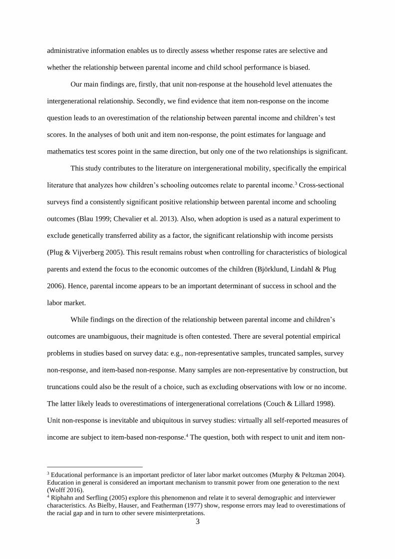
The box plots in Figure 3 provide a first insight into the test score distributions by income
group. They allow a comparison of the median, the 25th and 75th percentile, as well as the span of
Cito scores, between the different subgroups by response status. Differences between the groups can
be observed for all income quintiles. Across all income quintiles, the median student whose parents do
not respond performs worse than the median student whose parents respond. The same holds at the
75th percentile and, in the three lowest income quintiles, also for the 25th percentile of the distributions.
A Kolmogorov-Smirnov test on the underlying distributions shows that this difference is significant
for the third and fourth income quintile. Figure 3 confirms the finding shown in Table 1 that children
of non-responding parents perform significantly worse than those of responding parents. However,
these differences could be explained by differences with respect to background characteristics or
income levels. In the following, we therefore explore whether the gap in schooling outcomes between
children of responding and non-responding parents remains after controlling for demographics, and
income. As a basic set of controls, we use students’ gender and age as well as an indicator for low
socio-economic status.20
Table 5 shows the results of the main regression specifications, displaying only the income
coefficients. We run the same regression of students’ performance on the parental income quintile and
control (1) for the full sample and (2) for a number of artificially restricted samples. In a first step, the
full sample is split into students attending a non-responding school (NRS) or a responding school
(RS). In a second step, the sub-sample attending responding schools is split into parental response
status. This allows us to compare children of non-responding parents (NRP) to those of responding
parents (RP).
20 As indicated earlier, the latter variable is mainly based on whether the parents have a particularly low
educational background. It is our best available proxy for parental education background for the full sample,
including non-responding parents.

13
In this setup, comparing the NRP and RP samples shows the bias induced by individual unit
non-response.21 We repeat this analysis for three different schooling outcomes: (1) the total Cito score,
(2) the fraction of correct tasks in sub-sections for language, and (3) the fraction of correct tasks in
sub-sections for mathematics. All of these measures are standardized to a mean of zero and a standard
deviation of one. Thus, the resulting coefficients can be interpreted as a change in standard deviations,
associated with an increase of one quintile in income. P-values for the differences in the estimated
income coefficients, between non-responding and responding parents, are provided in the second panel
of Table 5.
All coefficients of the relationship between parental income quintile and students’ schooling
outcomes are significant at the 1 percent level.22 Regarding all three performance measures, the
coefficients for the sample with children of responding parents exceeds that for the sample with
children of non-responding parents in magnitude. However, none of these differences are significant.
A similar empirical approach, based on the full sample and the use of interaction terms between
different types of non-response and the income quintile, confirms these results (see Table A2). The
only significant differences between coefficients of intergenerational mobility in this sample are found
when analyzing institutional non-response (see appendix).
4.2 Parental unit non-response and item non-response in grade 9
We apply the same empirical strategy to the sample assessed in grade 9 (average age 15). In this wave,
the parental survey was sent out directly to parents, providing a direct measure of parental survey
response. This parental survey included a question regarding household income, allowing us to further
assess a potential bias due to specific item non-response.
In the following, we distinguish three groups: (1) children of parents who responded to the
survey and provided a measure of household income, (2) children of survey responders who did not
provide an income measure, and (3) children of survey non-responders.
21 The comparison between the coefficients of the NRS and RS samples provides a measure of whether and how
institutional unit non-response biases the estimate (see appendix for a discussion of the estimates). 22 All control variables, gender, age, and “low ses” (Socio-Economic Status) are significant. The coefficient for
low socio-economic background has a negative sign. Higher age is associated with a lower Cito score, most
likely because we are not able to control for grade retention. In addition, male students perform slightly better.

14
The box plots presented in Figure 4 show how achievement in the language test is distributed
within the different income quintiles, separately by parental response status. In general, the graph
reveals that the differences by participation status based on this test seem to be smaller than the
differences based on the Cito test in grade 6 (compare to Figure 3). A tendency towards positive
selection into survey response is observed. However, among children of survey responders,
particularly children of low-income parents who do not respond to the income question, outperform
the children of those who do respond, at most points in the distribution. The analog box plots for
achievement in the mathematics test in grade 9 are provided in the appendix, in Figure A3.
Applying the same approach used in the baseline sample, we examine whether unit and item
non-response bias the estimated relationship between parental income and children’s schooling. Table
6 displays the income coefficients of the main regression specification for the full sample as well as
artificially restricted sub-samples.
First, children are split according to whether their parents did (SR) or did not respond to the
survey (SNR). Then, children of survey respondents are distinguished by whether the parents did (IR)
or did not fill in the included income question (INR). Comparing the coefficients of the SNR and SR
samples provides a measure for unit non-response bias. A comparison between the INR and IR
samples provides insight into whether item non-response induces a bias. This analysis is conducted for
the language (1) as well as the mathematics achievement test (2), administered in grade 9 as part of the
OML.23 Both measures are standardized to a mean of zero and a standard deviation of one.
As can be seen in Table 6, the analysis based on the language test confirms the results from the
baseline sample for language scores: no significant evidence is found that unit non-response is a
source of bias in the estimated relationship between parental income and students’ language outcomes.
For mathematics, we do find significant differences. The estimate reveals that the relationship is
attenuated due to parental non-response. Regarding item non-response on income questions, we find
23 The difficulty level of the tests differs across schooling tracks, but with an overlap in questions. To place
students on one scale across schooling tracks we run a two-parameter item response theory model.

15
that the estimated relationship is biased upwards for language test scores. However, the difference is
not significant for mathematics test scores.24
Surprisingly, the estimated coefficient for parental income in the sample of item non-
responding parents is very small and insignificant. This observation may be explained by the contrast
between the two tests. The stakes of the Cito test, used in the baseline sample, are high as they partly
determine secondary school track placement. By contrast, the tests in grade 9 have no relevance for the
students in terms of grades or placement.
The availability of a self-reported and an administrative measure of parental income also
allows us to assess reporting bias in an intergenerational mobility setting: using survey-reported
income to measure intergenerational mobility (IGM), and then comparing the (potentially) “biased”
survey estimates with the “true” estimates using administrative measures of income. The results
indicate that the relationship between parental income and children’s educational outcomes is biased
when using self-reported measures of income. In our dataset, the relationship between self-reported
income and educational outcomes is not significant. Relative to the relationship between
administrative measures of income and educational outcomes, we can conclude that the results using
self-reported income are attenuated both for language (p-value .030) and for mathematics (p-value
.051).
4.3 Robustness checks
All of the above regression results rely on a corrected measure of household income, based on the total
household income adjusted for number of household members. As a robustness check, we conduct all
analyses also with the measure of total income. The results remain qualitatively similar but are
somewhat weaker in magnitude and significance. Since adjustment by number of household members
is highly relevant for the actual standard of living, this is not surprising. In support of this, for the sub-
24 We further discuss this in Section 5.2. An alternative approach, using interaction terms in a regression (see
Table A3), confirms the overestimation driven by item non-response. Applied to the difference between the
lowest and the highest income quintile, the induced bias amounts to more than half a standard deviation in the
language achievement test. It almost completely offsets the estimated positive association between parental
income and performance regarding the language test.

16
sample of parents with a known education level, we also find that the quintile of a household’s
corrected income correlates more strongly with highest education level than with total income.
The error terms of the test scores are unlikely to be independent across students in the same
environment. Attending the same school and having the same teacher could systematically influence
student achievement. Therefore, we account for common factors of influence in the results shown
above. To ensure that our results are not driven by clustering, we repeat all analyses with non-
clustered standard errors. We do not find any major difference to the results discussed above.
Significant differences in the fraction of immigrants in groups by response status raise the
question whether these could drive the reported results. In the appendix, we show estimates excluding
immigrants (Table A9 and A10). The coefficients are somewhat larger compared to the results based
on the full sample including immigrants. However, in a qualitative sense, the results on the differences
between the sub-groups by response status remain unchanged. Therefore, immigrants do not drive the
conclusions we draw.
5 Potential mechanisms
Our results indicate that individual unit and item non-response by parents may bias estimates in
opposite directions. In the following, we discuss potential mechanisms behind the underlying selection
into unit and item non-response in our samples.
5.1 Selection into individual unit non-response
The magnitude of the intergeneration mobility coefficient in the group of responding parents is, across
both age groups and for all outcome measures, consistently lower than in the group of non-responding
parents. Thus, individual unit non-response could potentially lead to an overestimation of
intergenerational mobility.
To get a better insight into the sorting of parents in terms of survey participation, we regress
parental survey response on individual student characteristics. The results are presented in the
appendix in Table A5. In both surveys, grade 6 and 9, being a first or second-generation immigrant is
associated with a lower probability of parental survey participation. Also, children’s academic

17
performance is related to a higher probability of parental response. In primary school, Cito scores
significantly predict parental response. In secondary school, the more recent performance measures are
more important. Attending a secondary school track other than the lowest one is associated with a
lower response rate among parents. However, this is conditional on all the other variables, and the
coefficient on having low-educated parents (“low ses”) is negative and exceeds any of the coefficients
on track. Again in the secondary school sample, parents in households not belonging to the lowest or
the middle income quintile are more likely to respond to the survey. Effects regarding school location
are no longer significant once a variable on the use of dialect is added. In both samples, speaking the
local dialect well is associated with a higher probability of parental survey response.
All in all, in both surveys the parents of well-performing students who are not immigrants and
who speak the local dialect well are more likely to answer. In the secondary school sample, socio-
economic background and track placement play an important role as well.
5.2 Selection into income item non-response
Among parents who return the survey but do not answer questions on household income, the
relationship between parental income and children’s language performance is weaker than among
parents who do respond to the question. The selection into item non-response could shed some light on
the potential mechanisms behind this bias.
While there is a positive selection into unit response with respect to parental education,
parental income, and students’ test scores, this is different for item non-response. As can be concluded
from the boxplot in Figure 4 (as well as Figure A3), children of low income item non-responders, in
particular, outperform those of item responders.
An explanation that fits in with this pattern is that parents with low income but otherwise
favorable characteristics25 may feel that they do not live up to expectations and are therefore reluctant
to report their income. This is consistent with non-responders having atypical characteristics for the
area they live in, as has been shown for the US census (Bee et al. 2016). Such a systematic item non-
25 Examples of individuals with low income but otherwise favorable characteristics would be a university
graduate with a degree in philosophy who works as a taxi driver, or individuals who are still completing their
education, such as PhD students.

18
response pattern is particularly harmful for estimates of intergenerational mobility. Since the non-
responders are atypical for the area they live in, imputation of missing data based on postal code area,
as applied by Sabelhaus et al. (2015), is risky.
An additional difference can be observed in the mode of responding to the survey. The
majority of item responders (88.9 percent) filled out the online survey to which a link was provided in
the initial invitation letter, while only 22.5 percent of item non-responders did so. Most of them (77.5
percent) instead filled out the paper survey which was only provided in the reminder letter. This points
towards a potential link between the mode of the survey, the willingness to respond to certain items,
and potentially further characteristics.
A regression of parental item response on individual student and parent characteristics can be
found in the appendix in Table A6. Student performance measures only positively significantly predict
parental item response if track and school location are not included. Parental item response is
dominantly associated with belonging to the highest income quintile26 and answering the survey upon
the first request online.
6 Conclusion
This paper assesses the potential bias in estimates of intergenerational mobility, specified as the
relationship between parental income and students’ school performance, combining administrative and
survey data. We identify different sources of non-response – parental unit and item non-response – and
show that they have to be considered separately because their effects on the estimates of
intergenerational mobility are distinct.
Our main results indicate, firstly, that unit non-response at the household level attenuates the
intergenerational relationship. Secondly, we find evidence that item non-response on the income
question leads to an overestimation of the relationship between parental income and children’s test
scores. In the analyses of both unit and item non-response, the point estimates for language and
mathematics test scores point in the same direction but only one of the two relationships is significant.
26 The coefficient indicating households in the middle income quintile most likely only becomes significant due
to the sample restriction from column (2) to column (3). Restricting the regressions in columns (1) and (2) in the
same way leads to significant coefficients as well.

19
These results are important both for the literature on intergenerational mobility but also for
that in other contexts. Non-response is ubiquitous and substantial in all estimations based on survey
data, e.g., among the articles we cite in our paper, non-response rates in other published studies on
intergenerational mobility are found of up to 42 percent. Our results suggest that estimates of
intergenerational mobility based on survey data need to be interpreted with caution because they may
be biased by selective non-response. The direction of such bias is difficult to predict a priori. Bias due
to unit and item non-response may work in opposing directions and may differ across outcomes.
Matching survey and administrative data enables us to directly assess the effects of non-
response. A remaining downside of our data set is the imperfect match of survey and performance data
to administrative data. Even though, at above 80 percent in the baseline sample, this match is
relatively high, it is not perfect. The remaining selection may drive our results to some extent.
To our knowledge, this is the first study on bias induced by selective unit and item non-
response in the important relationship between parental income and children’s school performance, as
an early measure of intergenerational mobility. Obviously, the results could be driven by the specific
setting of our study and as mentioned above, our results may partly be driven by incomplete matching
to administrative data. Therefore, this study needs to be replicated in different contexts. This is
feasible in countries where large administrative datasets are already available, for example in
Scandinavia. The same approach can of course be used to assess the bias induced by non-response in
any relationship of interest estimated based on survey data.
References
Bee, C. A., Gathright, G. & Meyer, B. D. (2016). Non-response bias in the measurement of income:
evidence from address linked tax records. Unpublished manuscript, presented at SOLE 2016.
Bielby, W. T., Hauser, R. M. & Featherman, D. L. (1977). Response errors of black and nonblack
males in models of the intergenerational transmission of socioeconomic status. American
Journal of Sociology 82(6), 1242-1288.
Björklund, A., Lindahl, M. & Plug, E. (2006). The origins of intergenerational associations: Lessons
from Swedish adoption data. The Quarterly Journal of Economics 121(3), 999-1028.

20
Black, S. E. & Devereux, P. J. (2011). Recent developments in intergenerational mobility. Handbook
of Labor Economics 4, 1487-1541.
Black, S. E., Devereux, P. J. & Salvanes, K. G. (2005). Why the apple doesn't fall far: understanding
intergenerational transmission of human capital. American Economic Review 95(1), 437-449.
Blau, D. M. (1999). The effect of income on child development. Review of Economics and Statistics
81(2), 261-276.
Bollinger, C. R. & Hirsch, B. T. (2013). Is earnings nonresponse ignorable? Review of
Economics and Statistics 95, 407-416.
Bollinger, C., Hirsch, B. T., Hokayem, C. & Ziliak, J. (2017). Trouble in the tails? What we know
about earnings nonresponse thirty years after Lillard, Smith, and Welch. Unpublished
manuscript.
Borghans, L., Korthals, R. & Schils, T. (2015). The effect of track placement on cognitive and non-
cognitive skills. Unpublished manuscript. Maastricht University.
Bound, J., Brown, C. & Mathiowetz, N. (2001). Measurement error in survey data. In: Heckman J.,
Leamer, E., eds. Handbook of Econometrics. Vol. 5. North-Holland; Amsterdam. 3705–3843.
Chevalier, A., Harmon, C., O’Sullivan, V. & Walker, I. (2013). The impact of parental income and
education on the schooling of their children. IZA Journal of Labor Economics 2(1), 1-22.
College voor Toetsen en Examens. (2015). Interpretatie van het leerlingrapport bij de centrale
eindtoets PO 2015. Utrecht: College voor Toetsen en Examens.
Corak, M. (2013). Income inequality, equality of opportunity, and intergenerational mobility. Journal
of Economic Perspectives 27(3), 79–102.
Couch, K. A. & Lillard, D. R. (1998). Sample selection rules and the intergenerational correlation of
earnings. Labour Economics 5(3), 313-329.
EUROSTAT (2009). Task force on the quality of the Labour Force Survey.
Hariri, J. & Lassen, D. (2017). Income and outcomes – social desirability bias distorts measurements
of the relationship between income and political behavior. Public Opinion Quarterly 81(2),
564–576.

21
Hauser, R. M. (2005). Survey response in the long run: The Wisconsin Longitudinal Study. Field
Methods 17(1), 3-29.
Inspectie van het Onderwijs. (2014). De staat van het onderwijs, onderwijsverslag 2012/2013.
Utrecht: Inspectie van het Onderwijs, Nederland.
Jäntti, M. & Jenkins, S. (2015). Income mobility. Handbook of Income Distribution. Atkinson, A. and
Bourguignon, F. (eds.). Vol. 2., 807-935.
Lillard, L., Smith, J. P. & Welch, F. (1986). What do we really know about wages? The importance of
nonreporting and census imputation. Journal of Political Economy 94(3), Part 1, 489-506.
Martikainen, P., Laaksonen, M., Piha, K. & Lallukka, T. (2007). Does survey non-response bias the
association between occupational social class and health? Scandinavian Journal of Public
Health 35(2), 212-215.
Micklewright, J. & Schnepf, S. V. (2006). Response bias in England in PISA 2000 and 2003 (Vol.
771). Department for Education and Skills.
Murphy, K. M. & Peltzman, S. (2004). School performance and the youth labor market. Journal of
Labor Economics 22(2), 299-327.
Nybom, M. & Stuhler, J. (2015). Biases in standard measures of intergenerational income dependence.
Journal of Human Resources, forthcoming.
Plug, E. & Vijverberg, W. (2005). Does family income matter for schooling outcomes? Using
adoptees as a natural experiment. The Economic Journal 115(506), 879-906.
Porter, S. R. & Whitcomb, M. E. (2005). Non-response in student surveys: the role of demographics,
engagement and personality. Research in Higher Education 46(2), 127-152.
Reijneveld, S. & Stronks, K. (1999). The impact of response bias on estimates of health care
utilization in a metropolitan area: the use of administrative data. International Journal of
Epidemiology 28(6), 1134-1140.
Riphahn, R. T. & Serfling, O. (2005). Item non-response on income and wealth questions. Empirical
Economics 30(2), 521-538.
Sabelhaus, J., Johnson, D., Ash, S., Swanson, D., Garner, T. I., Greenlees, J. & Henderson, S. (2015).
Is the Consumer Expenditure Survey representative by income? In C. D. Carroll, T. F.

22
Crossley & J. Sabelhaus (Eds.), Improving the measurement of consumer expenditures (Vol.
74, pp. 241-262). Chicago and London: University of Chicago Press.
Søgaard, A. J., Selmer, R., Bjertness, E. & Thelle, D. (2004). The Oslo Health Study: the impact of
self-selection in a large, population-based survey. International Journal for Equity in Health
3(1), 3.
Tourangeau, R. & Yan, T. (2007). Sensitive questions in surveys. Psychological Bulletin 133(5), 859–
883.
Turrell, G., Patterson, C., Oldenburg, B., Gould, T. & Roy, M.-A. (2003). The socio-economic
patterning of survey participation and non-response error in a multilevel study of food
purchasing behaviour: area-and individual-level characteristics. Public Health Nutrition 6(2),
181-189.
Wolff, M. C. (2016). Ernst und Entscheidung. Berlin: Nomos.

23
FIGURES AND TABLES
Figure 1 Data collection and response rates in both samples

24
Table 1 Descriptive statistics for students by survey response status, baseline sample grade 6 (age 12)
Note: The table reports the number of observations, the mean values and the standard deviations for the listed
variables by response status on the parental survey in grade 6 at age 12, conditional on having school
administrative information on the students and matched public administration information. The analysis is based
on those students for which all variables are available; the most restrictive being the Cito test scores. The
different sub-samples (1), (2), and (3) are mutually exclusive. Age is based on the students’ month-exact age at
the beginning of grade 6. Gender takes the value of 1 for male students and 0 otherwise. “Low ses” is an
indication used and provided by the school administration. Schools receive extra funding if the proportion of
students indicated as “low ses” exceeds a certain threshold. It is 1 if one or both of the parents did not complete
secondary education (this indication is comparable to the “free lunch” indication in the US). A child is
considered to have a migration background if at least one parent was not born in the Netherlands. Parental
education level relies on a self-reported measure and is therefore only available if the parental survey was
completed. It is coded in terms of the five levels defined in the International Standard Classification of Education
(ISCED). Corrected income is reported on the household level in terms of quintiles relative to the entire Dutch
population. It is based on the income register at 31 December 2008. The Cito test score reflects the overall score
including sections on language, mathematics and study skills. The information provided on the language and
mathematics sub-sections are reported in the percentage of questions answered correctly. Blanks indicate that the
data source of this variable is not available for the group in question.
Survey participation status
(1) (2) (3)
Survey participation School non-response Parental non-response
Variable N mean sd N mean sd N mean sd
Age (in years in grade six) 2,611 12.21 .54 373 12.27 .55 737 12.27 .54
Gender (fraction male) 2,722 .49 .50 429 .48 .50 780 .49 .50
Low ses (fraction) 2,611 .12 .33 373 .10 .31 737 .19 .39
Migration background (fraction) 2,722 .14 .35 428 .20 .40 777 .22 .42
Highest parental education (1-5) 2,681 3.25 1.09 0 . . 0 . .
Corrected HH Income (1-5) 2,709 3.05 1.32 426 3.13 1.36 767 2.81 1.35
Cito test score (500-550) 2,611 536.90 8.86 373 537.32 9.14 737 534.93 9.06
Cito test: language section (%) 2,611 77.19 11.16 373 77.88 11.64 737 74.85 11.70
Cito test: mathematics section (%) 2,611 73.50 16.95 373 73.74 16.98 737 70.64 17.00
General cognitive ability (0-43) 2,655 32.69 4.68 22 28.91 6.08 556 31.82 5.07
2,722 429 780
(1) vs. (2) (1) vs. (3) (2) vs. (3)
** ***
*** ***
*** ***
. . .
*** ***
*** ***
*** ***
*** ***
*** *** ***
* 5% ** 1% *** 0.1%

25
Figure 2 Students’ Cito score distributions by survey response status, baseline sample grade 6 (age 12)
Note: This graph is restricted to all students for whom Cito test scores were available and data could be merged
with administrative household information. The group with responding parents relates to column (1) from Table
1, the groups with non-responding schools and from non-responding parents correspond to columns (2) and (3),
respectively.

26
Table 2 Parental survey participation by income quintile, baseline sample grade 6 (age 12)
Note: The table shows survey participation rates by quintile of corrected income for the three groups
distinguished in Table 1. It includes all observations for which data from school administration and Cito test
scores are available and can be linked to administrative records of the parents.
Survey
participation
School
non-resp.
Parental
non-resp.Total
Lowest 423 73 170 666
15.61 17.14 22.16 17.07
Second 582 65 170 817
21.48 15.26 22.16 20.94
Third 609 105 166 880
22.48 24.65 21.64 22.55
Fourth 632 98 154 884
23.33 23.00 20.08 22.66
Highest 463 85 107 655
17.09 19.95 13.95 16.79
Total 2,709 426 767 3,902
100.00 100.00 100.00 100.00
Standardized
HH income
(quintile)
Survey participation status

27
Table 3 Descriptive statistics for students by survey response status, sample grade 9 (age 15)
Note: The table reports the number of observations, the mean values and the standard deviations for the listed
variables by response status on the parental survey at age 15, conditional on taking either a mathematics or
language test. The different sub-samples (1), (2), and (3) are mutually exclusive. Age refers to the students’
month-exact age at the beginning of grade 9. The variables gender, low ses, migration background, parental
education, income and Cito test were assessed in grade 6 and are the same as in Table 1. Gender takes the value
of 1 for male students and 0 otherwise. “Low ses” is an indication used and provided by the school
administration. Schools receive extra funding in case the proportion of students indicated as “low ses” exceeds a
certain threshold. It is 1 if one or both of the parents did not complete secondary education (this indication is
comparable to the “free lunch” indication in the US). A child is considered to have a migration background if at
least one parent was not born in the Netherlands. Parental education level relies on a self-reported measure and is
therefore only available if the parental survey was completed. It is coded in terms of the five levels defined in the
International Standard Classification of Education (ISCED). Corrected income is reported on the household level
in terms of quintiles relative to the entire Dutch population. It is based on the income register at 31 December
2008. The Cito test score reflects the overall score including sections on language, mathematics and study skills.
The variables language test and mathematics test refer to scores on tests conducted specifically for the OML.
The reported scores are standardized to a mean of zero and a standard deviation of one.
Survey participation status
(1) (2) (3)
Survey & item response Survey non-response Item non-response (1) vs. (2) (1) vs. (3) (2) vs. (3)
Variable N mean sd N mean sd N mean sd
Age (in years in grade six) 474 15.10 .41 1,682 15.20 .47 807 15.12 .46 *** ***
Gender (fraction male) 474 .46 .50 1,682 .49 .50 807 .48 .50
Low ses (fraction) 455 .04 .50 1,595 .17 .38 777 .07 .26 *** ** ***
Migration background (fraction) 474 .10 .30 1,680 .20 .40 806 .09 .29 *** ***
Highest parental education (1-5) 352 3.61 1.03 1,093 3.15 1.12 619 3.39 1.00 *** *** ***
Corrected HH Income (1-5) 472 3.51 1.24 1,669 2.88 1.33 804 3.18 1.27 *** *** ***
Cito test score (500-550) 455 539.70 7.82 1,595 535.98 8.95 777 537.76 8.63 *** *** ***
Language test, grade 9 (stand.) 363 .21 .99 1,268 -.08 .96 620 .14 .95 *** ***
Mathematics test, grade 9 (stand.) 360 .30 .93 1,269 -.13 .97 617 .16 .99 *** ***
General cognitive ability (0-43) 399 33.45 4.53 1,385 32.33 4.80 690 33.06 4.41 *** ***
474 1,682 807

28
Table 4 Parental survey participation by income quintile, sample in grade 9 (age 15)
Note: The table shows survey and item response rates by quintile of corrected income for the three groups
distinguished in Table 3. It includes observations for which data from school administration and test scores are
available and which can be linked to administrative records of the parents.
Survey and
item
participation
Survey
non-resp.
Item
non-resp.Total
Lowest 33 324 92 449
6.99 19.41 11.44 15.25
Second 75 371 174 620
15.89 22.23 21.64 21.05
Third 107 394 175 676
22.67 23.61 21.77 22.95
Fourth 130 337 222 689
27.54 20.19 27.61 23.40
Highest 127 243 141 511
26.91 14.56 17.54 17.35
Total 472 1,669 804 2,945
100.00 100.00 100.00 100.00
Standardized
HH income
(quintile)
Survey participation status

29
Figure 3 Box plots of students' Cito scores by survey response and income, baseline sample grade 6 (age 12)
Note: Box plots for Cito test results, displayed by survey response status and income quintile. The boxes are
drawn around the median, indicated by the line in the box, and show the interquartile range from the 25th
percentile to the 75th percentile. The whiskers show the span of the data points. Their maximum length is 1.5
times the interquartile range. Data points outside this span are usually displayed separately. In accordance with
the policy on non-disclosure of individual data by Statistics Netherlands, the figure does not include those
outside values (here: 24 observations). The graph is based on 2,602 students whose parents participated in the
survey, 726 students whose parents did not respond, and 371 students whose schools did not respond.

30
Table 5 Relationship between students’ test scores and parental income, different samples (grade 6)
Note: The table reports OLS regressions of children’s Cito test scores on parental income. Each cell represents a
separate regression. The dependent variables are total Cito scores as well as percentile scores on the sub-sections
language and mathematics, standardized to a mean of zero and a standard deviation of one. The coefficients
shown in each cell are those of the independent variable income, which is measured in quintiles, based on the
Dutch population. Income refers to corrected income, adjusted for the number of household members. Each
regression controls for a number of variables: age, gender, and indicators of low socio-economic status as well as
of first- or second-generation immigrant status. Standard errors are reported in parenthesis. They are clustered at
the school level (there are 174 schools). Significance levels are reported as follows: .1 *, .05 **, and .01 ***.
N
Full sample 3,699 .213 *** .205 *** .171 ***
(.000) (.000) (.000)
371 .284 *** .276 *** .228 ***
(.000) (.000) (.001)
3,328 .204 *** .196 *** .165 ***
(.000) (.000) (.000)
726 .217 *** .209 *** .168 ***
(.000) (.000) (.000)
2,602 .196 *** .187 *** .160 ***
(.000) (.000) (.000)
Wald test on income coefficients Hypothesis
School non-response NRS = RS .116 .035 ** .173
Parental non-response NRP = RP .502 .474 .758
Non-responding schools (NRS)
Responding schools (RS)
Non-responding parents (NRP)
Responding parents (RP)
p-values
Coefficients for income quintile
(1) (2) (3)
Cito test Language Mathematics

31
Figure 4 Box plots for students’ language test by survey response and income, sample grade 9 (age 15)
Note: Box plots for language test results in grade 9, displayed by survey response status and income quintile.
The boxes are drawn around the median, indicated by the line in the box, and show the interquartile range, from
the 25th percentile to the 75th percentile. The whiskers show the span of the data points. Their maximum length
is 1.5 times the interquartile range. Data points outside this span are usually displayed separately. In accordance
with the policy on non-disclosure of individual data by Statistics Netherlands, the figure does not include those
outside values (here: 34 observations). The graph is based on 356 students whose parents participated in the
survey, including the income question, 613 students whose parents responded to the survey without reporting
household income and 1,247 students whose parents did not return the survey.

32
Table 6 Relationship between students’ test scores and parental income, different samples (grade 9)
Note: The table reports OLS regressions of children’s language and mathematics scores on parental income.
Each cell represents a separate regression. The dependent variables are the fraction of correctly answered
questions on the tests, standardized to a mean of zero and a standard deviation of one. The coefficients shown in
each cell are those of the independent variable income, which is measured in quintiles, based on the Dutch
population. Income refers to corrected income. Each regression controls for a number of variables: age, gender,
and indicators of low socio-economic status as well as first- or second-generation immigrant status. Standard
errors are reported in parenthesis. They are clustered at the school and track level (there are 579 school-track
combinations. Significance levels are reported as follows: .1 *, .05 **, and .01 ***.
Coefficients for income quintile
N N
.122 *** 2,216 .152 *** 2,198
(.000) (.000)
.128 *** 1,247 .167 *** 1,241
(.000) (.000)
.087 *** 969 .093 *** 957
(.001) (.000)
.042 613 .080 ** 605
(.191) (.011)
.164 *** 356 .102 *** 352
(.000) (.005)
Wald test on income coefficients Hypothesis
Parental survey non-response SNR = SR .225 .020 **
Parental item non-response INR = IR .017 ** .643
Survey non-responding parents (SNR)
Survey responding parents (SR)
Item non-responding parents (INR)
Survey, and item responding parents (IR)
p-values
(1) (2)
Language Mathematics
Full sample

33
Appendix 1
Onderwijsmonitor Limburg
The OnderwijsMonitor Limburg (OML) is a collaboration between Maastricht University, educational
institutions (primary, secondary and tertiary) and government bodies in the Province of Limburg (in
the south of the Netherlands).
The OML aims to gain insights into the educational development of pupils/students in order to
foster the further improvement of education and the transition from education to the labor market in
the Province of Limburg, and to acquire knowledge about the dynamics of educational processes in
general.
More than 95 percent of all primary schools in the south of Limburg participate in this
education monitor. The project is approved by the local school boards of Limburg. Test scores are
processed by the MEMIC Maastricht (center for data and information management) in anonymized
form.
The key elements of the OML are:
- structural accumulation of relevant data throughout the educational career of pupils/students in
Limburg (longitudinal)
- effective dialogue and collaboration between the OML partners
- high-quality research (both academic and applied) and dissemination of insights into the
domains of academia, policy and educational practice.
The OML collects data regarding:
- cognitive pupil/student outcomes (school career and test results)
- non-cognitive pupil/student characteristics (primarily socio-emotional and socio-economic)
- parent and household characteristics
- teacher characteristics
- school characteristics
The starting point of the OML is information which is already collected within the schools.
Additional testing and surveying is done where needed (in close collaboration with the schools).

34
Earlier academic publications using data from the OML are:
Borghans, L., Golsteyn, B., Zölitz, U. (2015). School quality and the development of cognitive skills
between age four and six. PLOS ONE 10(7), e0129700.
Feron, E., Schils, T., ter Weel, B. (2016), Does the teacher beat the test? The additional value of the
teacher's assessment in predicting student ability. De Economist 164(4), 391-418.
Golsteyn, B., Schils, T. (2014). Gender gaps in primary school achievement: A decomposition into
endowments and returns to IQ and non-cognitive factors. Economics of Education Review 41,
176-187.
Künn-Nelen, A., de Grip, A., Fouarge, D. (2015). The relation between maternal work hours and the
cognitive development of young school-aged children. De Economist 163(2), 203-232.

35
Appendix 2
Institutional selective non-response
In this appendix, we discuss the results with respect to selective institutional non-response.
Figure 3 shows that students attending non-responding schools mostly outperform students with
responding parents at the lower end of the test score distribution. However, in the lowest income
quintile, the variance is larger for students in non-responding schools. In the highest income quintile,
students at non-responding schools outperform both other groups across the full distribution.
Table 5 reveals that the largest coefficients, i.e., the lowest intergenerational mobility, can be
observed for the sample of non-responding schools. A quantitative comparison of the coefficients
across the samples shows that only the difference induced by institutional unit non-response is
significant. From separate regressions for performance in language and mathematics, it becomes
apparent that the bias is more strongly driven by differences in the language sub-section of the Cito
test. Table A2 confirms these findings. The interaction term between income quintile and school non-
response for total Cito scores or the language sub-section is significant at the 5 and in some cases the 1
percent level. Again, this is different for mathematics scores. The magnitude of this interaction effect
amounts to more than half of the income quintile coefficient. When applying this to the difference
between the lowest and the highest income quintile, the gap in the estimates for children of responding
parents and non-responding schools amounts to about a third of the standard deviation in Cito test
scores. Using probability weights to account for differential participation based on the parental income
group cannot correct this bias.
In sum, regarding institutional unit non-response by schools, we find evidence for a significant
overestimation of intergenerational mobility.
What are the potential underlying mechanisms? The fourteen schools which did not send out
the parental surveys show a stronger relationship between parental income and children’s schooling
outcomes than responding schools. This could either be explained by differences in characteristics, by

36
anticipation of parental response behavior, or because the schools may use non-response as a strategy
to avoid unfavorable results. These explanations are discussed in the following.
All of the non-responding schools except for one are Roman Catholic, as are the majority of
primary schools in the sample. Table 1 shows that significantly fewer students from a low socio-
economic background attend non-responding schools, while more first or second-generation
immigrants attend such schools. This combination of characteristics would be consistent with a large
fraction of children of academically trained expats in the student population.27 Furthermore, while the
students at non-responding schools on average score higher on the Cito test, they also have a higher
standard deviation. The same holds for parental income. With the favorable selection of student
population and high average performance, non-responding schools are unlikely to attract the attention
of the Inspectorate of Education. However, they seem to be of low quality in terms of addressing
intergenerational mobility.
Should the schools be aware of this, a potential explanation for their non-response could be
that they do not want to disclose this weakness. Similarly, the extent of participation in the research
project could be positively related to how much schools care about equality of opportunity. This
comparison of responding and non-responding schools is purely descriptive and unconditional. A
regression of school participation on aggregated characteristics (see Appendix, Table A4) does not
show any significant relationship with the above-mentioned characteristics. However, schools in two
of the regions are significantly more likely to participate.
School non-response could also be driven by anticipated parental non-response. That is,
schools may not respond because they assume that parents would not be willing to participate in the
surveys. Since the survey in grade 9 is sent out directly to the same parent population, we can check
whether there is a basis for this assumption. The differences in parental response behavior that we find
are very small. Parents whose children attended a non-responding primary school seem to be even
more willing to participate in surveys and to provide complete information. So if schools do not
respond because they thought parents in the school would not want to, their assumption is incorrect.
27 This group of immigrants is overrepresented in the south of Limburg due to the presence of Maastricht
University as well as some international chemicals companies.
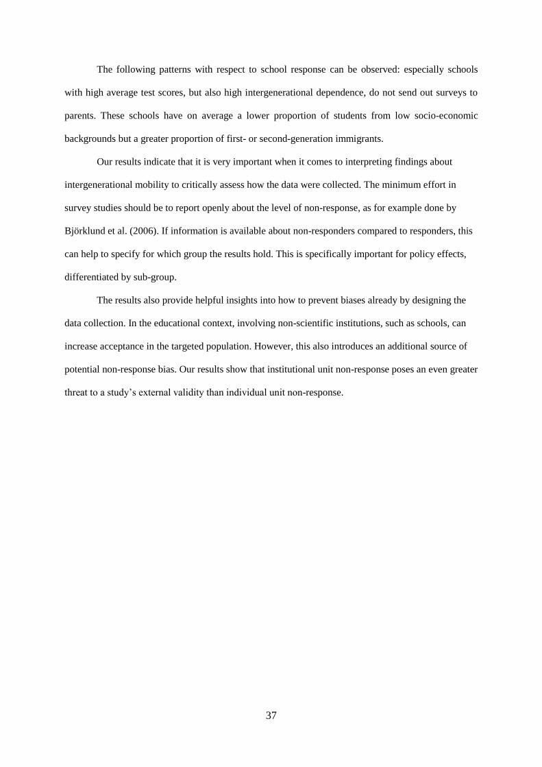
37
The following patterns with respect to school response can be observed: especially schools
with high average test scores, but also high intergenerational dependence, do not send out surveys to
parents. These schools have on average a lower proportion of students from low socio-economic
backgrounds but a greater proportion of first- or second-generation immigrants.
Our results indicate that it is very important when it comes to interpreting findings about
intergenerational mobility to critically assess how the data were collected. The minimum effort in
survey studies should be to report openly about the level of non-response, as for example done by
Björklund et al. (2006). If information is available about non-responders compared to responders, this
can help to specify for which group the results hold. This is specifically important for policy effects,
differentiated by sub-group.
The results also provide helpful insights into how to prevent biases already by designing the
data collection. In the educational context, involving non-scientific institutions, such as schools, can
increase acceptance in the targeted population. However, this also introduces an additional source of
potential non-response bias. Our results show that institutional unit non-response poses an even greater
threat to a study’s external validity than individual unit non-response.

38
Appendix 3
Additional tables and graphs
Table A1 Descriptive statistics for students without administrative data, baseline sample grade 6 (age 12)
Note: The table reports the number of observations, the mean values and the standard deviations for the listed
variables by response status on the parental survey in grade 6 at age 12 for all students for whom data could not
be merged to administrative data from the income registry. The different sub-samples (1), (2), and (3) are
mutually exclusive. Age is based on the students’ month-exact age at the beginning of grade 6, their final year in
primary education. Gender takes on the value 1 for male students. “Low ses” is an indication used and provided
by the school administration. Schools receive extra funding in case the proportion of students indicated as “low
ses” exceeds a certain threshold. It is 1 if one or both of the parents did not complete secondary education (this
indication is comparable to the “free lunch” indication in the US). A child is considered to have a migration
background if at least one parent was not born in the Netherlands. Parental education level relies on a self-
reported measure and is therefore only available if the parental survey was completed. It is coded in terms of the
five levels defined in the International Standard Classification of Education (ISCED). Corrected income is
reported on the household level in terms of quintiles relative to the entire Dutch population. It is based on the
income register at 31 December 2008. The Cito test score reflects the overall score including sections on
language, mathematics and study skills. The information provided on the language and mathematics sub-sections
are reported in percent of questions answered correctly. Blanks indicate that we do not have information on the
variable for that particular group.
Survey participation status
(1) (2) (3)
Survey participation School non-response Parental non-response
Variable N mean sd N mean sd N mean sd (1) vs. (2) (1) vs. (3) (2) vs. (3)
Age (in years in grade six) 510 12.26 .59 50 12.28 .64 227 12.38 .61 ***
Gender (fraction male) 536 .51 .50 73 .62 .49 247 .60 .49 **
Low ses (fraction) 512 .19 .39 50 .02 .14 229 .21 .41 *** ***
Migration background (fraction) 600 .19 .39 . . . . . . . . .
Highest parental education (1-5) 578 3.04 1.08 . . . . . . . . .
Total Income (1-5) . . . . . . . . . . . .
Corrected HH Income (1-5) . . . . . . . . . . . .
Cito test score (500-550) 512 534.16 9.24 50 536.36 8.67 229 532.78 10.17 * **
Language test, grade 9 (stand.) 512 74.00 11.71 50 76.52 10.42 229 71.83 13.12 ** **
Mathematics test, grade 9 (stand.) 512 69.17 17.74 50 73.66 17.27 229 68.25 18.37 * *
General cognitive ability (0-43) 575 31.70 4.99 - - - 195 31.41 4.74 . .
601 73 267

39
Figure A1 Students’ language test distributions by survey response status, sample grade 9 (age 15)
Note: This graph shows the distribution of students’ language achievement test, standardized to a mean of zero
and a standard deviation of one. It is based on all grade 9 students for whom data could be merged with
administrative household information and who took the language achievement test. The group with responding
parents who answered the income question relates to column (1) from Table 3, the group with non-responding
parents correspond to column (2), and responding parents who do not answer the income question, the item non-
response group, relate to column (3).

40
Figure A2 Students’ mathematics test distributions by survey response status, sample grade 9 (age 15)
Note: This graph shows the distribution of students’ mathematics achievement test, standardized to a mean of
zero and a standard deviation of one. It is based on all grade 9 students for whom data could be merged with
administrative household information and who took the language achievement test. The group with responding
parents who answered the income question relates to column (1) from Table 3, the group with responding
parents who do not answer the income question, non-responding parents correspond to column (2), and the item
non-response group, relates to column (2).

41
Table A2 Regression results for full sample with interactions, baseline sample 6 (age 12)
Note: The table reports OLS regressions of children’s Cito test scores on parental income. The dependent
variables are (1) overall Cito test scores and respectively sub-scores on the (2) language and (3) mathematics
section, standardized to a mean of zero and a standard deviation of one. Income refers to corrected income. Each
regression includes controls for a number of gender, students’ month-exact age, and indicators of low socio-
economic status as well as of first- or second-generation immigrant status. Standard errors are reported in
parentheses. Significance levels are reported as follows: .1 *, .05 **, and .01 ***.
School (S) non-response -.231 * -.231 -.193 -.193 * -.224 * -.224
(.133) (.145) (.134) (.110) (.134) (.143)
Parental (P) non-response -.165 * -.165 -.172 * -.172 * -.108 -.108
(.092) (.106) (.093) (.099) (.094) (.096)
Income quintile .147 *** .147 *** .143 *** .143 *** .124 *** .124 ***
(.014) (.014) (.014) (.014) (.014) (.014)
Income * S non-response .086 ** .086 *** .081 ** .081 *** .073 * .073 **
(.038) (.032) (.039) (.029) (.039) (.033)
Income * P non-response .007 .007 .013 .013 -.004 -.004
(.029) (.031) (.029) (.030) (.029) (.028)
Controls X X X X X X
Clustered s. e. X X X
R² .152 .152 .136 .136 .130 .130
N 3,699 3,699 3,699 3,699 3,699 3,699
Test scores
(1) (2) (3)
Cito test Cito test Language
(sub-section)
(4) (5) (6)
Language
(sub-section)
Mathematics
(sub-section)
Mathematics
(sub-section)

42
Figure A3 Box plots for students’ mathematics test by survey response and income, sample grade 9 (age 15)
Note: Box plots for mathematics test results in grade 9, displayed by survey response status and income quintile.
The boxes are drawn around the median, indicated by the line in the box, and show the interquartile range, from
the 25th percentile to the 75th percentile. The whiskers show the span of the data points. Their maximum length
is 1.5 times the interquartile range. Data points outside this span are usually displayed separately. In accordance
with the policy on non-disclosure of individual data by Statistics Netherlands, the figure does not include those
outside values (here: 20 observations). The graph is based on 425 students whose parents participated in the
survey, including the income question, 717 students whose parents responded to the survey without reporting
household income and 1,527 students whose parents did not return the survey.

43
Table A3 Regression results for full sample with interactions, ssample grade 9 (age 15)
Note: The table reports OLS regressions of children’s Cito test scores on parental income. The dependent
variables are (1) overall Cito test scores and respectively sub-scores on the (2) language and (3) mathematics
section, standardized to a mean of zero and a standard deviation of one. Income refers to corrected income. Each
regression includes controls for a number of gender, students’ month-exact age and indicators of low socio-
economic status as well as first- or second-generation immigrant status. Standard errors are reported in
parentheses. Significance levels are reported as follows: .1 *, .05 **, and .01 ***.
Parental survey (P) non-response .008 .008 -.480 *** -.480 ***
(.164) (.170) (.156) (.144)
Item (I) non-response .389 ** .389 ** -.062 -.062
(.179) (.186) (.173) (.164)
Income quintile .134 *** .134 *** .074 * .074 **
(.040) (.043) (.038) (.036)
Income * P non-response -.045 -.045 .057 .057
(.045) (.047) (.043) (.041)
Income * I non-response -.127 ** -.127 ** -.015 -.015
(.049) (.051) (.048) (.046)
Controls X X X X
Clustered s. e. X X
R² .096 .096 .104 .104
N 2,120 2,120 2,094 2,094
(1) (2)
Language Language
Test scores
Mathematics Mathematics
(3) (4)

44
Table A4 Regression of school survey response on aggregate characteristics
Note: The table reports coefficients of Probit regressions. The dependent variable is school survey response. The
independent variables include: the fraction of male students, the fraction of students with at least one parent who
did not complete secondary education; the fraction of students who are first- or second-generation immigrants;
the fraction of students, belonging to households of the indicated income quintile, based on corrected income;
the average, the standard deviation of the Cito score and the correlation between income quintile and Cito test
scores within each school; and indicators for school location (the baseline being north Limburg). Standard errors
are reported in parentheses. Significance levels are reported as follows: .1 *, .05 **, and .01 ***.
Gender (fraction, males) -.292 -.696 -.943
(1.194) (1.321) (1.381)
Low ses (fraction) 1.470 1.974 1.599
(1.481) (1.829) (1.834)
Migration background (fraction) -.977 -.921 -.696
(1.595) (1.765) (1.864)
Income quintile 2 (fraction) 3.019 4.868 * 5.171 *
(2.114) (1.555) (2.676)
Income quintile 3 (fraction) -.249 .191 .427
(1.788) (2.010) (2.162)
Income quintile 4 (fraction) 1.111 1.118 1.135
(1.835) (2.088) (2.214)
Income quintile 5 (fraction) .548 .164 .348
(1.946) (2.166) (2.230)
Cito test score (500-550), average -.007 .006 .004
(.061) (.065) (.066)
Cito test score (500-550), standard deviation -.029 -.036 -.026
(.106) (.117) (.119)
Correlation: income quintile & Cito test score -.502
(.673)
Location: Westelijke Mijnstreek 2.179 ** 2.353 **
(.995) (1.033)
Location: Parkstad 1.278 1.412
(.872) (.891)
Location: Maastricht / Heuvelland 2.049 *** 2.194 **
(.933) (.966)
Pseudo R² .069 .163 .170
N 174 171 170
(1) (2) (3)
School survey response

45
Table A5 Regression of parental survey response on individual characteristics
Note: The table reports coefficients of Probit regressions. The dependent variable is parental survey response.
The independent variables included for both samples are: a variable indicating male students, an indicator for
students with at least one parent who did not complete secondary education; an indicator for students being first
or second-generation immigrants; indicators for the quintile of corrected income the households belongs to; the
student’s Cito test score; indicators for school location (with the baseline being north Limburg); and an indicator
for speaking the local dialect well. Additionally, for the sample of secondary school students, a combined
performance measure of the language and mathematics tests in grade 9, as well as indicators for the attended
track (the baseline being the two lower pre-vocational tracks, VMBO b/k), are included. Standard errors are
reported in parentheses. Significance levels are reported as follows: .1 *, .05 **, and .01 ***.
(4)
Gender (male = 1) -.013 -.013 .002 -.053 -.008 -.027
(.049) (.049) (.055) (.049) (.049) (.055)
Low ses -.099 -.072 -.132 -.431 *** -.377 *** -.440 ***
(.077) (.077) (.085) (.088) (.090) (.100)
Migration background -.241 *** -.237 *** -.131 * -.327 *** -.355 *** -.329 ***
(.069) (.069) (.078) (.075) (.075) (.086)
Income quintile 2 .091 .097 .079 .256 *** .262 *** .307 ***
(.078) (.079) (.088) (.086) (.086) (.094)
Income quintile 3 .071 .062 .045 .159 * .151 * .085
(.081) (.081) (.090) (.085) (.086) (.095)
Income quintile 4 .103 .087 .041 .354 *** .298 *** .306 ***
(.082) (.083) (.092) (.086) (.087) (.096)
Income quintile 5 .125 .112 .125 .342 *** .272 *** .321 ***
(.091) (.092) (.104) (.092) (.093) (.103)
Cito test score (500-550) .011 *** .012 *** .010 *** .014 *** -.012 ** -.014 **
(.003) (.003) (.003) (.003) (.005) (.005)
Language & mathematics, grade 9 .247 .267 **
(.163) (.181)
Track: pre-vocational (VMBO g / t) .162 * .128
(.086) (.095)
Track: higher general (HAVO) .533 *** .554 ***
(.100) (.110)
Track: academic (VWO) .698 *** .739 ***
(.121) (.133)
Location: Westelijke Mijnstreek -.493 ** -.256 -.093
(.232) (.250) (.172)
Location: Parkstad -.507 ** -.396 -.096
(.230) (.247) (.170)
Location: Heuvelland -.280 -.174 .005
(.234) (.252) (.173)
Location: Maastricht -.502 ** -.470 * -.180
(.238) (.256) (.184)
Speaking dialect well .255 *** .131 **
(.059) (.058)
Pseudo R² .015 .020 .031 .043 .055 .071
N 3,328 3,321 3,034 2,813 2,813 2,349
Parental survey response
(1) (3) (5) (6)
Baseline survey, grade 6 (age 12)
(2)
Sub-sample, grade 9 (age 15)

46
Table A6 Regression of parental item response on individual characteristics
Note: The table reports coefficients of Probit regressions. The dependent variable is parental item response. The
independent variables included are: a variable indicating male students, an indicator for students with at least one
parent who did not complete secondary education; an indicator for students being first or second-generation
immigrants; indicators for the quintile of corrected income the households belongs to; the student’s Cito test
score; z-standardized performance measures of the language and mathematics tests in grade 9; indicators for the
attended track (the baseline being the two lower pre-vocational tracks, VMBO b/k); indicators for school
location (with the baseline being north Limburg); and an indicator for speaking the local dialect well. Standard
errors are reported in parentheses. Significance levels are reported as follows: .1 *, .05 **, and .01 ***.
Gender (male = 1) -.135 -.127 -.061 -.098
(.104) (.105) (.116) (.137)
Low ses -.067 -.034 .041 -.273
(.224) (.230) (.257) (.313)
Migration background .053 .044 .017 .061
(.175) (.175) (.195) (.233)
Income quintile 2 .130 .113 .200 .333
(.201) (.202) (.222) (.275)
Income quintile 3 .310 .299 .471 ** .609 **
(.199) (.199) (.222) (.276)
Income quintile 4 .258 .229 .321 .274
(.192) (.193) (.214) (.261)
Income quintile 5 .559 *** .534 *** .663 *** .972 ***
(.200) (.201) (.223) (.271)
Cito test score (500-550) .018 ** .010 .012 .010
(.007) (.011) (.012) (.014)
Language test, grade 9 (stand.) -.040 -.047 -.040 -.070
(.061) (.062) (.068) (.082)
Mathematics test, grade 9 (stand.) -.020 -.038 -.045 -.119
(.061) (.064) (.071) (.086)
Track: pre-vocational (VMBO g / t) .145 .169 .085
(.208) (.223) (.276)
Track: higher general (HAVO) .134 .129 .226
(.232) (.250) (.305)
Track: academic (VWO) .299 .202 .272
(.274) (.297) (.363)
Location: Westelijke Mijnstreek .122 .489
(.326) (.403)
Location: Parkstad .023 .365
(.320) (.397)
Location: Heuvelland -.078 .046
(.325) (.399)
Location: Maastricht -.054 .107
(.353) (.430)
Speaking dialect well -.061 .096
(.123) (.148)
Response to first / online survey 1.982 ***
(.149)
Pseudo R² .028 .030 .032 .350
N 650 650 548 548
(1) (2) (3) (4)
Parental item response

47
Table A7 Relationship between students’ test scores and parental income, different samples (grade 6), no
controls
Note: This table is similar to Table 5. Here, the estimations are performed without controls.
N
Full sample 3,699 .213 *** .205 *** .171 ***
(.000) (.000) (.000)
371 .284 *** .276 *** .228 ***
(.000) (.000) (.001)
3,328 .204 *** .196 *** .165 ***
(.000) (.000) (.000)
726 .217 *** .209 *** .168 ***
(.000) (.000) (.000)
2,602 .196 *** .187 *** .160 ***
(.000) (.000) (.000)
Wald test on income coefficients Hypothesis
School non-response NRS = RS .116 .035 ** .173
Parental non-response NRP = RP .502 .474 .758
Non-responding schools (NRS)
Responding schools (RS)
Non-responding parents (NRP)
Responding parents (RP)
p-values
Coefficients for income quintile
(1) (2) (3)
Cito test Language Mathematics

48
Table A8 Relationship between students’ test scores and parental income, different samples (grade 9), no
controls
Note: This table is similar to Table 6. Here, the estimations are performed without controls.
Coefficients for income quintile
N N
.122 *** 2,216 .152 *** 2,198
(.000) (.000)
.128 *** 1,247 .167 *** 1,241
(.000) (.000)
.087 *** 969 .093 *** 957
(.001) (.000)
.042 613 .080 ** 605
(.191) (.011)
.164 *** 356 .102 *** 352
(.000) (.005)
Wald test on income coefficients Hypothesis
Parental survey non-response SNR = SR .225 .020 **
Parental item non-response INR = IR .017 ** .643
Survey non-responding parents (SNR)
Survey responding parents (SR)
Item non-responding parents (INR)
Survey, and item responding parents (IR)
p-values
(1) (2)
Language Mathematics
Full sample

49
Table A9 Relationship between students’ test scores and parental income, different samples (grade 6), no
migrants
Note: This table is similar to Table 5. The estimations are performed on a sample excluding immigrants.
N
Full sample 3,119 .154 *** .151 *** .132 ***
(.000) (.000) (.000)
309 .198 *** .208 *** .182 ***
(.001) (.000) (.002)
2,810 .148 *** .144 *** .126 ***
(.000) (.000) (.000)
569 .151 *** .147 *** .115 ***
(.000) (.000) (.000)
2,241 .145 *** .142 *** .127 ***
(.000) (.000) (.000)
Wald test on income coefficients Hypothesis
School non-response NRS = RS .217 .112 .204
Parental non-response NRP = RP .860 .892 .742
Non-responding schools (NRS)
Responding schools (RS)
Non-responding parents (NRP)
Responding parents (RP)
p-values
Coefficients for income quintile
(1) (2) (3)
Cito test Language Mathematics

50
Table A10 Relationship between students’ test scores and parental income, different samples (grade 9), no
migrants
Note: This table is similar to Table 6. The estimations are performed on a sample excluding immigrants.
Coefficients for income quintile
N N
.084 *** 1,817 .122 *** 1,779
(.000) (.000)
.091 *** 976 .159 *** 951
(.000) (.000)
.069 ** 841 .071 *** 828
(.014) (.006)
.027 532 .065 ** 525
(.422) (.052)
.149 *** 309 .081 *** 303
(.001) (.040)
Wald test on income coefficients Hypothesis
Parental survey non-response SNR = SR .525 .010 ***
Parental item non-response INR = IR .027 ** .748
Survey non-responding parents (SNR)
Survey responding parents (SR)
Item non-responding parents (INR)
Survey, and item responding parents (IR)
p-values
(1) (2)
Language Mathematics
Full sample