Working paper (submitted for review to the journal Wind Energy)

Comparing empirical and simulated wind speed and power data

June 29, 2012 Authors: Todd Ryan1,2, William Buchanan1,3, Paul D. H. Hines*3, Paulina Jaramillo2,

Gabriela Hug2 Abstract Using data from two large US wind interconnection studies and two grid-scale wind power plants, this paper provides evidence that mesoscale meteorological models under-predict the variability in wind speeds, but for large wind farms the power production data have more similar statistics. Specifically, the mesoscale models under-predict the high-frequency variability in wind speeds, as measured by the power spectral density and the probability of large changes in wind speeds. However, these differences only appear to translate into an under-prediction of power production variability when modeling small wind plants (less than 10 square miles in area), where the effect of geographic diversity is minimal. When modeling larger wind plants, the filtering of the power output due to geographic diversity roughly offsets the filtering effect of the mesoscale model on predicted wind speeds. The exception to this is that the simulated data consistently under-predict the probability of very large wind ramping events, such as a 50% change in power output over an hour. The results show some evidence that methods aimed at correcting the reduced variability may result in too much high-frequency variability. We conclude that while meteorological models are important for large-scale wind integration studies, caution is needed for analyses that could be sensitive to the probability of large ramping events and high-frequency variability. 1. Introduction The desire to reduce dependence on fossil fuels and mitigate anthropogenic climate change is resulting in numerous policy incentives for renewable energy. Since wind generation is arguably the most affordable of the new renewable energy options, wind generation capacity quadrupled between 2004 and 2008 [1]. With this rapid increase in wind generation comes the need to better understand the impact that the variability and intermittency of wind generation have on the reliability of the power grid. As a result, numerous large-scale wind integration studies produced by government, industry, and academic organizations have worked to estimate the reliability impacts of large-scale wind power and the feasibility of various levels of wind power production [2]-[9]. However, estimating the impact of large amounts of new wind energy production in systems that currently have only a small number of existing wind plants requires an                                                                                                                1  These authors contributed equally to this work * Corresponding Author: Paul.Hines@uvm.edu 2 T. Ryan, P. Jaramillo, and G. Hug are with Carnegie Mellon University. 3 W. Buchanan and P. Hines are with the University of Vermont.

 

  2  

estimate of the time-varying output from power plants that do not yet exist. Such estimates typically require large amounts of predicted wind speed data for hypothetical wind farm locations, which are then transformed to produce estimates of wind power output. Once generated, these large quantities of spatially diverse wind power production data can be used to answer a wide variety of cost and reliability questions, using different types of analytical methods, along different time scales. The most straight-forward use of wind data is to estimate the total quantity of annual or seasonal energy in a region or across a set of locations. However, wind integration studies frequently seek to understand not only the energy impacts, but also the costs associated with wind variability, which has different characteristics at different time scales. Along monthly to yearly time scales, wind data can be used to estimate the seasonal or inter-annual variability in wind plant production. Along multiple-day time horizons, the data can feed unit commitment models, which can estimate the impact of hourly wind plant variability on energy market dispatch costs. Along time horizons of minutes to hours, simulated wind plant data can be used to estimate the need for load following generation resources or generation reserves. Higher resolution data can be used to estimate the requirements for regulation and frequency management as a function of wind power deployment. There are, however, limited quantities of appropriately accurate empirical wind speed data available to those seeking to produce wind integration studies. The US National Weather Service collects large amounts of anemometer data [10],[11]. These data are collected at 10 meter elevations, which reduces their utility for studying wind turbines with hub heights of 80 meters and higher. Furthermore, wind speed data are typically archived at 10-15 minute intervals, which means that they cannot easily be used to solve problems that require higher sample rate data. Some 50-100 meter wind speed data exist, typically in connection with site evaluation studies for new wind power plants, but only for a small number of locations, and the data are not generally publically available for statistical analysis. Data from existing wind plants provide a more accurate understanding of the statistical properties of wind plants, since they are not subject to the above uncertainties. However, extrapolating from data at one location to produce wind speed or power data for a non-existent wind plant at a distant location will result in errors, since wind patterns are different in different regions and topographies. In addition, the reliability impacts of large-scale wind deployment will depend highly on the correlations between wind output and demand for electricity. In some locations wind is correlated with daily load patterns, whereas in others, wind is anti-correlated. Because of the difficulty in obtaining empirical wind speed data, almost all large-scale wind integration studies use simulated wind speed data from meteorological models known as mesoscale Numerical Weather Prediction (NWP) models. NWP models are calibrated to approximately reproduce historical meteorological measurements, such as wind vectors, cloud cover, and precipitation using data assimilation methods [12]-[14]. Such models are termed mesoscale because they are designed to model spatial and

 

  3  

temporal patterns between those of synoptic scale models, which model global climate patterns with lower spatial resolution, and microscale models, which focus on spatial resolutions of less than 1 km. Mesoscale models have sufficient spatial resolution to estimate wind speeds at several elevations and locations with approximately 2-10 km spatial resolution. Computer-based NWP models have been used for meteorological analysis since the late 1970s and currently there are two widely used models: Mesoscale Model Version 5 (MM5) [15],[16] and the Weather Research and Forecasting (WRF) model [17]. A detailed review of mesoscale modeling methods and tools is available in [14]. While accurate wind speed data are a necessary input for most large-scale wind integration studies, wind speed data alone are not sufficient. In order to estimate the power output from potential future wind plants, speed data need to be translated into estimates of wind power production using wind power curves for a particular turbine. The International Electrotechnical Commission has developed a standard function for mapping wind speeds to wind power, using the wind turbine manufacturer’s provided power curve and site specific wind speed data (i.e., IEC 61400-12) [18],[19]. However, this method was developed to test and predict the performance of a single turbine and may not produce an accurate estimate for wind plant production due to variations in wind speeds across the wind plant; i.e., the modeled power output from a wind plant with n turbines will not exactly match n times the modeled output from one wind turbine. Wind speeds within a wind plant will not be perfectly correlated, particularly at short time scales or in locations with variable terrain. Though non-deterministic power curves have been used in some studies (e.g., the SCORE method in Potter et al. [20]), using such models adds model complexity, and introduces additional uncertainty into the data. For this reason, integration studies generally use a deterministic power curve. Given the substantial importance of wind integration studies to long-term policy decisions, and the importance of mesoscale model data to these studies, there is value in better understanding similarities and differences between the simulated data and data from real wind farms. Therefore, the goal of this research is to identify the extent to which wind speed data from meteorological models, and the resulting simulated wind power output, show the statistical characteristics of empirical wind speed and power data. 2. Data 2.1. Wind power plant data We make use of wind speed and power production data from two wind plants located in the central United States.3 The first (Plant A) is a large plant with approximately 300 MW in capacity. The second (Plant B) is smaller, with a 120 MW capacity. Plant A consists of over 250 wind turbines (approximately 300 MW capacity) and two meteorological towers. The wind speed data are taken at a height of 80 meters and are

                                                                                                               3  The exact locations cannot be revealed per the terms of non-disclosure agreements.  

 

  4  

averaged over ten-minute intervals. The wind power data are also averaged over ten-minute intervals, and are metered individually for each turbine, as well as for the entire plant. In order to understand how wind power statistics change with plant size, the data for Plant A were parsed into six sets based on increasing distance to the northwestern meteorological tower. These sets consist of 1, 10, 50, 100, 200, and all turbines, respectively, as described in Table  1, and are referred to as Plant A - set 1, … , Plant A - set 6. The area of each set was estimated based on the rectangle defined by the extreme latitudes and longitudes of each set. The area for Plant A - set 1 was assumed to be 0.001 km2, the area of a single turbine as estimated by the National Renewable Energy Laboratory (NREL) [22]. The power for each set was the sum of all turbines in the set, which created six unique time-series of wind power production. Parsing and aggregating the data in this way essentially created empirical data for six wind plants of increasing size and allowed us to study the effect of geographic diversity on the variability of the wind plant power production. Table 1: General Characteristics of the sets created from Plant A. A map of the plant is available at [37].

Set Number Number of Turbines Area Covered (km2) Plant A-Set 1 1 0.001 Plant A-Set 2 10 7.7 Plant A-Set 3 50 51.8 Plant A-Set 4 100 124.3 Plant A-Set 5 200 194.25 Plant A-Set 6 256 285

The second empirical dataset came from a smaller wind plant (Plant B) consisting of 80 turbines with a peak production capacity of 120 MW. The dataset includes only power output, sampled at 2-second time intervals, for the entire wind plant. Wind speed data were not available for Plant B. Each of the data sets used in this paper included some errors or anomalies that needed correction. For details on these errors and their corrections, please refer to the appendix (A.2 Data errors and corrections). 2.1. Meteorological modeled wind speed and power data The simulated wind speed and power data for this research were obtained from publicly available data associated with the Eastern Wind Integration Study (EWITS) [2] and the Western Wind and Solar Integration Study (WWSIS) [4]. These two studies were coordinated by NREL in 2010 and looked at the operational impacts of large-scale integration of wind energy across the U.S. Each of the EWITS and WWSIS datasets contains three years of wind speed and wind power data for potential wind plant locations in the U.S., both land-based and off-shore. The EWITS dataset consists of 10-minute

 

  5  

wind speed and plant output values for 1,326 simulated wind plants, based on simulated data for 2004-2006. EWITS also provides next-day, six-hour, and four-hour wind production forecasts for each simulated wind plant at hub heights of 80- and 100-meters. The MM5 model with a 2 km spatial resolution produced these predicted wind speeds. The WWSIS dataset consists of three years (2004-2006) of 10-minute simulated wind speed and plant output values for 32,043 simulated locations at a hub height of 100 meters. WWSIS does not provide forecast data. The WWSIS data come from the WRF model, also with 2 km grid spacing. The WWSIS and EWITS datasets use different methods to transform wind speed data into wind plant power output data. Most of the sites in the EWITS dataset represent wind plants between 100 MW and 600 MW in size, whereas each site in the WWSIS dataset represents the power output from ten Vestas V90 3-MW turbines. The EWITS power data were produced using a deterministic power curve that was the composite of multiple manufacture’s power curves [21]. WWSIS provides three different output power datasets for each site. The first transforms the wind speed data with a deterministic power curve. The remaining methods use statistical techniques (termed SCORE and SCORE-lite), which were designed using data from wind speed and power data from several existing wind plants [20]. The SCORE technique, or Statistical Correlation to Output from Record Extension, was designed to correct for some of the statistical smoothing that results from the use of mesoscale NWP models. SCORE-lite is a less complex version of the more detailed SCORE algorithm [20]. A detailed analysis of the power time-series data produced by the SCORE method can be seen in Milligan et al. [33], where the SCORE and SCORE-lite data are compared to data from an existing wind farm. 3. Data Analysis Methods This paper employs two methods for quantifying the variability in wind speed and power data. Sections 3.1 and 3.2 discuss the power spectral density approach, which allows one to measure the magnitude of variability at different time scales. Section 3.3 discusses the step-change analysis method, which allows one to see the frequency at which changes of various magnitudes occur. 3.1. Power spectral density analysis method The statistical properties of wind speeds are well documented in the literature. For example, Tuller and Brett [23] showed that the Weibull distribution can be used to model the relative occurrence of winds with various speeds. While the absolute probability density of wind speeds is important for estimating energy production, for wind integration studies that deal with reliability issues, the amount of change in wind power that result from changes in wind speeds will be of greater importance. Power spectrum analysis provides a useful method for measuring the quantity of variability in time-series data at different time scales. The power spectral density (PSD, or power spectrum) for a stream of time-domain data x(t) indicates the amount of variability in x at each frequency for which the PSD was calculated (see the appendix for details on PSD calculations). Traditionally PSDs are calculated for either voltage or power signals resulting in units of

 

  6  

V2Hz-1 or W2Hz-1 depending on the source. The analysis presented in this paper includes the PSD of wind speed data, with units of m/s; therefore the units resulting from this analysis will be in (m/s)2Hz-1. The PSD of wind power data, also included in this paper, is reported in units of (capacity)2Hz-1. For wind speed data, it is well known that atmospheric turbulence gives rise to a Kolmogorov distribution in the power spectrum of wind speeds [24]-[25]. Kolmogorov found that the relative variability (power) of turbulent flows decreases with the 5/3rds power of the frequency. Several recent articles have shown that wind speeds follow the Kolmogorov spectrum over a large range of frequencies [26]-[31]. While the configuration and size of a wind plant will have some effect on the power spectrum of wind power production from a wind plant, wind speed data from any location should have a power spectral density (PSD), y(f), that fits well to a model of the form in equation 1, with ! ! "5 / 3 , for frequencies (f) between 10-6 and 10-2 Hz.

y( f ) = cf ! (1)

where c is a scaling constant. More practically, this means that for each doubling in frequency, the amount of signal power (the average of the square of the data) in this frequency range decreases by a factor of 25/3 (3.17). Thus, the amount of signal power in the vicinity of one cycle per hour (2.8x10-4 Hz) is about 3 times larger than the amount of power in the range of one cycle per half hour (5.6x10-4 Hz). As a result of the Kolmogorov spectrum, changes in wind speeds at different time scales have fat-tailed probability density functions [31]. For this paper, we analyzed wind speeds for EWITS land-based 80- and 100-meter hub heights (1,326 sites); as well as 3,200 WWSIS sites (~10%). The WWSIS subset of sites was carefully checked to ensure that no one geographic region was overly represented in the sample. Both WWSIS and EWITS include three years of data in separate files, which we combine into a single wind speed time series for each site and hub height. We use Bartlett’s method for segment averaging [32] when calculating the PSD of a site. This method minimizes the effect of noise on the data without dampening the actual signal variance. To implement Bartlett’s method, we divide our time-series data into 30 equally sized data segments (10 segments per year) and calculate the PSD for each segment. Each of these PSD values is subsequently averaged at each frequency to obtain an average power spectrum for each site. If yi ( f ) is the PSD for segment i at frequency f, the

average spectral density ( y( f ) ) is:

y( f ) = 130

yi ( f )2

i=1

30

! (2)

The appendix includes a discussion of different approaches to power spectral analysis, and their impact on the outcomes (A.1 Spectral Analysis). Using these spectra, we use

 

  7  

least squares estimation on log(y( f )) to find the exponent α and offset c from equation 1 for each site. 3.2. Model fitting to find the point at which PSD of wind speeds diverges from the Kolmogorov Our initial analysis of the EWITS and WWSIS datasets indicated that there are distinct frequency ranges with different statistical properties within the data (see Figure 3). The PSDs of the wind speeds from the mesoscale models match the Kolmogorov spectrum for a range of low frequencies, but for higher frequencies the spectral densities fall faster than the f -5/3 line. Identifying the frequency at which the slope change occurs allows us to identify the frequency range in which the simulated wind speed data diverge from the PSD of real wind speed data. In order to estimate the frequency at which this change in slope occurs, we fit the data to a model (! ! ) of the following form:

y( f ) =c1 f

!1, fl < f < fkc2 f

!2 , f ! fk

"#$

%$ (3)

where α1 and α2 are the low and high frequency exponents, c1 and c2 are scaling constants, fm is a minimum frequency below which the Kolmogorov spectrum does not apply, and fk is the “knee” frequency at which the change in slope is estimated to occur. To ensure that y( f ) was not discontinuous at the knee point, we calculate the scaling parameter c2 to solve:

c1 fk!1

c2==

c2 fk!2

c1 fk!1!!2 (4)

We identified ordinary least squares estimates for the slope and scaling parameters for a range of fk values and chose fk to be the value that minimized the mean squared error for the model (Eq. 3) as a whole. In other words, the parameters result from solving for fk in equation 5.

c1,!1,!2 , fkmin log y( fi, fk,c1,!1,!2 )( )! log y( fi )( )( )

2

i=1

N

"

(5)

where N is the number of frequencies in the PSD, fi represents an individual frequency within the PSD calculation, and y(...) represents the estimated PSD, based on equations (3)-(4). 3.3. Step-change analysis method

 

  8  

The PSD method allows one to measure the relative magnitude of variability at different time scales, but does not give one much information about how frequently changes of a certain size occur. Knowing how frequently large step changes (such as a 50% reduction in power output in a ten minute period) occur can be useful in estimating the reliability impact of large wind plants in a particular area, as well as estimating the amount of fast-ramping generation needed to balance supply and demand. To implement the step-change method [31],[38],[39], we calculated average wind speeds and power production for 10-minute and 1-hour time intervals, and then computed the difference between adjacent intervals. For the absolute value of the step-changes from each dataset previously described, we computed complementary cumulative distribution functions (CCDF). In order to compare the empirical and mesoscale model data we identified sites from the EWITS or WWSIS that are in close proximity to the locations of Plant A and Plant B. We then compared the CCDF of the empirical data to that of our proximate simulated sites under the assumption that the proximate sites have similar geography and therefore should have similar statistical characteristics. Differences between the CCDFs of the empirical power plants and proximate simulated plants were noted in order to better understand differences between the empirical and simulated data. For Plant A, we compared the data to data from the six closest EWITS and the three closest WWSIS sites, all of which are less than thirty miles from the site for Plant A. For Plant B we compared the empirical data to data from the three closed EWITS sites, all of which are less than 20 miles away. 4. Results 4.1. PSD analysis results for wind speed data The PSD analysis results on the wind speed data show a number of interesting patterns. The single slope least squares fit (equation 1) for the PSD of the anemometer data from Plant A yielded a power-law slope of α=-1.68. As one would expect from previous literature [26],[31], the power spectral density of the anemometer data from Plant A follows the Kolmogorov slope over a large frequency range (Figure  1).

 

  9  

 Figure 1: Power spectral density diagram of empirical wind speeds from an anemometer at 80 m elevation located at Plant A, along with the fitted power-law slope, which is close to the Kolmogorov spectrum of f-5/3. In contrast, the PSD of the wind speed data from EWITS and WWSIS do not follow the Kolmogorov spectrum well; this can be seen in Figure  2, which shows the average power spectral density results for EWITS and WWSIS (both at 100 m), along with the fitted lines from equations (1) and (3). A substantial difference between the single log-linear fit and the Kolmogorov spectral density data is clear. In order to more clearly highlight the frequency range over which the data follow the Kolmogorov spectrum, Panels C and D show the same PSD data after dividing by f

-5/3. Data that follow a Kolmogorov spectrum, when normalized in this way would fall along a horizontal line. Panels E and F of Figure  2 show the results from fitting the PSDs with separate slopes above and below the knee frequency fk. In this case, the model fit is improved, as reflected by the decrease in the mean squared error from 0.032 to 0.0097. For frequencies between 10-6 and fk the NWP wind speed data follow the Kolmogorov spectrum closely. This is apparent for all three datasets, with both EWITS datasets (80- and 100-m) showing a slope of α1 = -1.63, and with α1 = -1.65 for WWSIS (See Table 2). This indicates that mesoscale models at this spatial and temporal resolution approximately reproduce the statistics of wind speed variability for frequencies less than one cycle per 3-6 hours. However, for frequencies above one cycle per 6 hours the spectral density decreases with f

-2.36 for both EWITS and WWSIS. Table 2 gives the fit parameters for these results.

 

  10  

 Figure 2: Power spectral density results for 80 m hub height wind speed data from EWITS (right) and 100m hub height wind speeds from WWSIS (left). Panels (A) and (B) show the unsegmented PSD results along with the Kolmogorov spectrum (red lines) and the linear best fit (green lines). Panels (C) and (D) show the segment-averaged PSDs divided by f-5/3, with the horizontal line showing the Kolmogorov spectrum. Panels (E) and (F) represent the segmented PSD results and the best-fit slopes for frequencies greater and less than the calculated fk value for the given dataset. Table 2: Parameter estimates for the EWITS and WWSIS wind speed spectral density models

EWITS, 80m height

EWITS, 100m height

WWSIS, 100m height

Single Slope* (α) -2.23 -2.25 -2.23 Model error (MSE**) 0.0341 0.0361 0.0301

Low Frequency Slope* (α1) -1.63 -1.62 -1.65 High Frequency Slope* (α2) -2.37 -2.39 -2.36 Model error (MSE ) 0.0089 0.0097 0.0075

Knee Frequency 4.70×10!! Hz 4.50×10!! Hz 4.50×10!! Hz *Single Slope refers to frequencies from f =10-6 to the Nyquist frequency (8x10-4 Hz), from Eq. 1. Low Frequency Slope refers to frequencies below the knee frequency (10-6<f < fk); High Frequency Slope refers to frequencies between the knee frequency and the Nyquist frequency (fk ≤ f ≤ 8x10-4). **  MSE:  Mean  Squared  Error  for  the  logarithmic  model  

 

  11  

Figure 3: Boxplot depicting all calculated single power-law exponents (α from Eq. 1) for each wind speed dataset with a 95% confidence interval.

To visualize the diversity among the various sites, Figure  3 shows the distributions of single power-law exponent estimates (α  from  equation  1)  of all individual sites for the three datasets (EWITS at 80m, EWITS at 100m, and WWSIS). This shows that all sites have average slopes that are well below the f -5/3, represented by the solid red line within the boxes, while also illustrating that the average slopes are approximately the same for all three datasets. The reduction in spectral density due to the divergence from the Kolmogorov spectrum will have only a small effect on wind speed variability at time scales in the range of 3-6 hours, but will have a more substantial effect at higher frequencies. In order to quantify the magnitude of this effect, we followed the following procedure. Given a spectral density y, equation (6) gives the reduction in spectral density between a knee frequency (e.g., fk ≅ 6-1 hours-1) and an arbitrary frequency, fh, above the knee.

y( fh )y( fk )

=c2 fh

!2

c2 fk!2=

fhfk

!

"#

$

%&

!2

(6)

To find the loss in spectral density at frequency fh that results from the exponent !!2 being steeper than !2 , we can use (6) to obtain:

!y( fh )y( fh )

=fhfk

!

"#

$

%&

!2 fhfk

!

"#

$

%&

' !!2

=fhfk

!

"#

$

%&

!2' !!2

(7)

 

  12  

This assumes that ! !! = !(!!), as is the case for our model. Equation 7 gives the relative change in spectral density at fh, due to the steeper slope !!2 . Thus, Eq. 7 indicates that with !!2 = 2.4 the power spectral density for 15-minute cycles (fh = 1.1x10-3 Hz) is reduced by a factor of 0.097, or by roughly 90%. An order-of-magnitude reduction in spectral density is substantial, indicating that the simulated wind speed data include a notable reduction in variability at higher frequencies. 4.2. PSD analysis results for wind power data To complement the wind speed PSD analysis, we also computed the PSD for the wind power production data from the EWITS and WWSIS datasets, as well the data from Plants A and B. First, Figure 4 shows the results for the segment-averaged PSD analysis for the power output of the entire EWITS and WWSIS datasets, along with their corresponding linear best-fit lines. This figure shows that the spectral densities for the power output from both EWITS datasets (80 and 100-meter hub heights) and the deterministic power curve of the WWSIS dataset are similar, whereas there is significantly more high-frequency variability within the SCORE-lite data. The difference between the deterministic and SCORE-lite data is not surprising, given that the purpose of SCORE-lite is to add variability at high frequencies in order to compensate for the averaging of the NWP models.

 Figure 4: Power spectral density results for 80 and 100m hub height wind power data from EWTIS (right) and 100m hub height wind power data, deterministic and SCORE-lite, from WWSIS (left). Each dataset also is shown with its corresponding linear best-fit line (green lines)

 

  13  

In the next step of our analysis, we compared the PSD of the power production data from Plants A and B with the corresponding geographically proximate EWITS and WWSIS sites. These exponents essentially describe the ratio of high-frequency variability to low-frequency variability shown in the power production data. Figure 5 shows the results for the segment-averaged PSD analysis for the power output of Plant A-Set 6 (as well as the linear best fit line of Plant A-Set 1) and Plant B, compared to the best-fit lines of the corresponding proximate EWITS and WWSIS sites. Unlike with the wind speed data, the PSD exponents from the EWITS and WWSIS data do not show a substantial underestimation of high-frequency variability, relative to the combined power production data from the Plant A (Set 6). In fact, the ratio of high-to-low frequency variability in WWSIS is substantially higher than what we find in the empirical data. Plant A-Set 6 has notably less high-frequency variability relative to the WWSIS deterministic and (particularly) the SCORE-lite data. The spectral characteristics of the EWITS data actually match those from the whole of Plant A quite well. Comparing the Plant A-Set 6 results with those from Plant A-Set 1 illustrates how decreasing the plant size increases the high-frequency variability in the power production data. This averaging effect results from increasing geographical diversity, and thus meteorological diversity, that can occur even within even a single wind plant. Table 3 shows this decreasing variability by tabulating the linear best-fit slopes of all 6 sets of Plant A. It is notable that the ratio of high-to-low frequency variability in the stochastic SCORE-lite data exceeds that found even in the data from a single turbine (Set 1). This seems to suggest that the SCORE-lite power curve introduces more variability into the data than what one would find in an actual power plant. Together these results suggest that the power production data from WWSIS contain more high-frequency variability than what is found in Set 6 of Plant A, but less high-frequency variability than Set 1. On the other hand, the EWITS data have similar spectral characteristics to those of the empirical data for the full plant (Set 6).

 

  14  

 Figure 5: Power spectral density results for wind power data from Plant A (top) and wind power data from Plant B (bottom), compared to the corresponding linear best fit lines from the EWITS and WWSIS datasets

 Table 3: Linear best fit slopes for the power spectral density data from Plant A

Set Number Power-law Best Fit for PSD

Plant A-Set 1 -1.8185 Plant A-Set 2 -2.1088 Plant A-Set 3 -2.3639 Plant A-Set 4 -2.4908 Plant A-Set 5 -2.5652 Plant A-Set 6 -2.5949

4.3. Step change analysis results for wind speed data In order to better understand the reduced variability indicated by the PSD analysis, this section compares empirical and simulated wind speed data using the step-change analysis method. Figure  6 compares the probability of 10-minute and 1-hour step changes of the real wind speeds from Plant A to those in wind speeds from proximate sites in the EWITS and WWSIS data. The probabilities of 2-6 m/s changes in wind speeds in the EWITS and WWSIS simulated 10-minute data are substantially (almost an order of magnitude) smaller,

 

  15  

relative to the empirical 10-minute data. This is to be expected based on the PSD analysis, which showed reduced variability in the EWITS and WWSIS datasets at high frequencies. For larger step changes (greater than 7 m/s) the WWSIS and empirical data show similar probabilities, whereas the EWITS data continue to show less variability. As one would expect from the PSD analysis, when the wind speeds are averaged over hourly time intervals, the differences between the simulated and empirical data are less obvious. The hourly step-change probabilities are a factor of 2-5 reduced in the simulated data, relative to the empirical data.

Figure 6: Complimentary Cumulative Probability Distribution Function (CCDF) for step-changes in wind speed for data from Plant A and the nearest EWITS and WWSIS plants, for 10-minute (above) and 1-hour (below) averages. Each point shows the probability of an absolute change that is greater than or equal to the value on the X-axis. 4.4. Step change analysis results for wind power data The second step-change analysis compared the variability of real wind power to that of wind power data from simulated wind plants. Figure 7 and Figure 8 compare the step change data for Plants B and A, respectively, with their geographically proximate

 

  16  

counterparts from the EWITS and WWSIS data. (Plant B is presented first because less data are available for that location.) The data in Figure 7 for Plant B indicate that the EWITS dataset somewhat under-predicts power output change occurrences. For example, the observed probability of a 10% or larger change in power output over a 10-minute interval is approximately 0.06 for the real wind plant, while the probability of the same change in the EWITS data is less than 0.02. A 50% change in the power output over 10 minutes is one half as likely in EWITS, relative to Plant B (0.0004 and 0.0002, for Plant B and EWITS proximate site, respectively). Similarly, a 10% change in power output over one-hour is 1.5 times less likely in EWITS than in the empirical data (0.30 verses 0.20 for Plant B and EWITS, respectively). Finally for a 50% change in one-hour power output, EWITS is 2 times less likely (0.0015 and 0.0030 for EWITS data and Plant B, respectively).

 Figure 7: CCDF comparison of the real wind power output of Plant B and its nearest EWITS plant for step changes of 10 minutes and 1-hour respectively. Figure 8 shows a similar comparison for Plant A, but with separate results for the single turbine (set 1), 50 turbine (set 3) and full power plant (set 6) cases (see Table  1). It is interesting to note that the relative accuracy of the mesoscale model data varies depending on which subset of turbines from Plant A one looks at. Ten-minute step changes of all sizes are substantially more probable in the single turbine case (set 1), relative to the EWITS data. On the other hand, the probabilities of large (greater than 70%) 10-minute step changes in the WWSIS data actually exceed those observed in Plant A - set 1. The differences in 10-minute step changes are less apparent for the 50-turbine (Plant A - set 3) case, but are still notable.

 

  17  

Figure 8: CCDF comparison of the real wind power output of Plant A, the synthetic wind power from its nearest EWITS plant, and the synthetic wind power from its nearest WWSIS plant for both deterministic and SCORE-lite power curves at uniform step changes of 10 minutes (upper panel) and 1 hour (lower panel) respectively. For the 1-hour step change analysis the results change. The step change probabilities in the WWSIS wind power data show higher step-change probabilities, relative to the data from Plant A – Set 6. The EWITS data, however, substantially underestimate the frequency of larger ramp events. The probability of a 60% or greater change is an order of magnitude lower in the EWITS data, relative to Plant A-Set 6. This difference is likely the result of extreme weather events, such as dramatic wind changes, which occur more gradually over time in mesoscale meteorological models. The differences between the EWITS and WWSIS data appear to result from a combination of differences in the meteorological models (WRF, which was used for WWSIS, is generally considered to be a more advanced model), and from the SCORE method that was used to stochastically translate wind speeds into power plant outputs in WWSIS. The data in Figure 8 highlight the impact of the SCORE-lite algorithm on the step-change probabilities, in the WWSIS data. For a step change greater than 70% of capacity in the

 

  18  

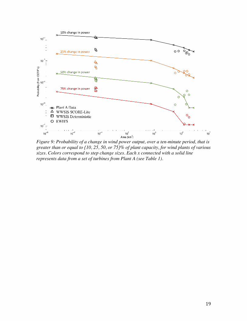
10-minute data, both the deterministic and SCORE-lite data produce step change probabilities that are greater than those seen in the Plant A-Set 3 and Plant A-Set 6. The deterministic WWSIS probabilities are similar to set 6 below a step change of 5%, and then higher than the empirical probabilities above a step change of 5% over a 10-minute period. At an hourly level, the affects of the SCORE-lite seem to be insignificant when compared to the deterministic values for the WWSIS set. Finally,  it  is  worth  noting  the  differences  in  the  tails  of  the  probability  distributions  (above  60%  step  changes).  The  WWSIS  data  substantially  overestimate  step-­‐change  probabilities  in  the  tails  of  both  the  10-­‐minute  and  one-­‐hour  data,  even  when  compared  to  a  single  turbine  (Plant  A  -­‐  set  1,  which  is  the  most  variable  set  from  Plant  A).  On  the  other-­‐hand,  the  data  from  EWITS  seem  to  underestimate  the  likelihood  of  large  step-­‐changes,  particularly  at  the  one-­‐hour  time  scale.  For  example,  the  EWTIS  site  shown  in  Figure  8,  did  not  contain  any  step  changes  greater  than  80%  of  capacity  for  the  1-­‐hour  data.  However,  empirical  data  suggest  that  very  large  step  changes  do  occasionally  occur. A key factor that is not captured particularly well in Figure 7 and 8 is wind plant size. Sets 1, 3, and 6 from Plant A are approximately 1, 50, and 300 MW, respectively; Wind Plant B is 120 MW; the EWITS approximate sites vary from 300 to over 800 MWs, while WWSIS sites are all 30 MW. In Figure 8 one can see how the CCDF of Plant A changes with additional turbines (i.e., from set 1 to set 3, set 3 to set 6; refer to Table  1); this is most evident in the 10-minute data (top of Figure 8). As more turbines are added, the distribution of Plant A converges with the proximate simulated EWITS data. In the final set, consisting of all the turbines in Plant A, the simulated 10-minute data for the EWITS site has more variability than the empirical 10-minute data of the entire plant (Plant A - set 6). In analyzing the wind speed data we focused on the effect of the smoothing of the mesoscale model on the synthetic data. The convergence of the step-change probability distributions with increasing number of turbines suggests that geographic diversity substantial reduces plant variability, even within a single power plant. In order to more carefully measure this “geographic smoothing,” Figure 9 and Figure 10 compare the relationship between plant size (in geographic area) and step change probabilities for both mesoscale-base simulated data and in empirical data. These figures plot the likelihood of a given sized step-change in power output for the different samples against the estimated area of each of these sample wind plants. Figure 9 is comprised of 10-minute data while Figure 10 uses 1-hour data.  From  these  figures,  it  can  be  seen  that,  in  general,  the  larger  the  area  of  the  wind  farm,  the  closer  most  step-­‐change  probabilities  from  the  simulated  data  come  to  the  corresponding  step-­‐change  probabilities  in  the  empirical  data.  Though  this  is  not  always  the  case  (see  50%  change  in  power  for  10-­‐minute  step-­‐changes),  this  holds  true  for  most  10-­‐minute  and  one-­‐hour  step  changes.  

 

  19  

 Figure 9: Probability of a change in wind power output, over a ten-minute period, that is greater than or equal to {10, 25, 50, or 75}% of plant capacity, for wind plants of various sizes. Colors correspond to step change sizes. Each x connected with a solid line represents data from a set of turbines from Plant A (see Table 1).

     

 

  20  

 Figure 10: Probability of a change in wind power output, over a one-hour time period, that is greater than or equal to {10, 25, 50, or 75}% of plant capacity, for wind plants of various sizes. Colors correspond to step change sizes. Each x connected with a solid line represents data from a set of turbines from Plant A (see Table 1).  4. Discussion The results presented in this paper indicate that mesoscale meteorological modes models, which are frequently used for large-scale wind integration studies such as EWITS and WWSIS, underestimate the variability in wind speed for frequencies above one cycle per 3 hours. The simulated wind speed data begin to diverge from the Kolmogorov power spectral density at about one cycle per 6 hours. This divergence is relatively small for frequencies below one cycle per 3 hours, but for higher frequencies, the difference is substantial and appears to result in notable differences between the wind speed variability observed at anemometers at actual wind plants and the wind speeds at simulated wind plants from the same geographic location. The results from our comparison of power production data for simulated and real wind farms are more nuanced. The simulated wind farms in the EWITS data show substantially lower 10-minute step change probabilities relative to actual data from small to medium sized wind farms. The EWITS 1-hour step-change probability distributions match well to those from real wind farms, except for very large (>50%) step changes. Results from the WWSIS data are less consistent; the comparison between the 10-minute deterministic and SCORE-lite WWSIS plant data showed that the deterministic power curve produced

 

  21  

results consistent with empirical data for small (>10%) step changes, while the SCORE-lite power curve tended to overestimate the probability observed for all step changes in the 10 minute time frame. Meanwhile the WWSIS 1-hour step-change probability distributions for both the deterministic and SCORE-lite power curves match well to real data for step changes up to 40%, after which the WWSIS over predicts step changes. We thus suggest that analysts should exercise caution before drawing broad conclusions when using simulated wind power data to answer grid reliability and wind intermittency questions that pertain to time scales under 3 hours. Milligan et al. [33] made a number of similar comparisons between empirical wind plants and mesoscale model wind power time-series produced by the WWSIS SCORE power curve. Their paper concludes that the SCORE and SCORE-lite predicted wind power had too much variability, as compared to geographically proximate (real) wind plants. The paper implies that this additional variability is due to the mesoscale model. The WWSIS data that they report are comparable to the data that are graphed as triangles in Figure  9:  . If the mesoscale modeling of wind speeds were the root cause of the additional variance seen in the SCORE and SCORE-lite data, then this additional variance would be observable in the PSD of the wind speeds. In fact, our PSD analysis of wind speeds shows that WWSIS data substantially underestimate the variability in wind speeds at higher frequencies. We thus suggest that the over-prediction of variability reported by Milligan et al. results from the method by which the wind speed data are translated into power production data. This is consistent with our results, which indicate that the stochastic SCORE-lite power curve used in WWSIS produces substantially more high frequency wind power variability, than what is found in actual wind farms. 5. Conclusions and Recommendations This work provides evidence that simulated wind power data derived from meteorological models can be reasonably used to answer some questions related to large-scale integration of wind resources, but is notably inadequate for others. For example, our results highlight the fact that fast wind ramping events that are caused by vertical atmospheric mixing are difficult to predict in mesoscale modeling [35] and are a real-world example of what conditions lead to the tails of the distribution of the step-changes in power. These types of fast-ramping events, the subsequent grid reliability impacts, and the ultimate costs of the reserves needed to mitigate such events would not be well predicted by data from meteorological models. On the other hand, modeled data like those used in EWITS and WWSIS are likely sufficient to evaluate the need for slower time-scale (hourly or greater) load-following resources that are needed with large-scale wind energy development. This work suggests several directions for future research. One area for potentially fruitful future work would be to improve the mesoscale models such that the wind data produced deviate less from the Kolmogorov spectrum. However, there is a combination of factors inherent to mesoscale models that collectively make it difficult to obtain better results for faster time scales. First, some of the input data for mesoscale reanalysis models include

 

  22  

fewer than 4 samples per day. As a result, reanalysis cases will naturally interpolate between these points, producing smoothing relative to empirical data. Second, the mesoscale (2 km) grid spacing will make it difficult to model atmospheric turbulence. Because turbulence occurs over spatial scales less than 2 km, and across complicated geographic features, mesoscale models will always smooth out changes in wind speeds to some extent. Microscale models, also known as Large Eddy Simulation models, are able to capture faster and more fine-grained spatial phenomena, and thus may produce more accurate wind speed data. This suggests that mesoscale models might be useful in combination with microscale models to produce data that have accurate statistics at multiple time scales. The framework of multi-scale modeling [34] may guide future work in this area. It is important to recognize that even though the EWITS and WWSIS data are not in complete agreement with empirical data, they currently include the best data publically available to researchers. While datasets of this sort should be used cautiously for decision-making, they are crucial for research and development. Similar datasets for wind power production do not exist. As new wind projects are developed and wind penetration increases, it is critical that empirical data be made available for research. In order to solve wind integration problems along shorter time scales, high-resolution (sample frequency of greater than one datum per minute) wind speed and wind power production data should be made publically available through the utilities or independent system operators. Such data could be used to improve the understanding of challenges and opportunities for wind power integration. Acknowledgement This work was funded in part by the RenewElec project at Carnegie Mellon University with the support from the Doris Duke Charitable Foundation, The Richard K. Mellon Foundation, The Heinz Endowment, The Electric Power Research Institute, The National Energy Technology Laboratory, and the Carnegie Mellon Electricity Industry Center. The results and opinions are the sole responsibility of the authors. The authors gratefully acknowledge those involved in making the data for this project publicly available. The datasets EWITS and WWSIS datasets were produced by the National Renewable Energy Laboratory, which is operated by the Alliance for Sustainable Energy, LLC for the U.S. Department Of Energy. Use of the data is subject to the user agreement, which is available at http://www.nrel.gov/wind/integrationdatasets/western/disclaimer.html. We also thank the wind plant operators that provided the data for Plants A and B. The raw operational data are protected by non-disclosure agreements. Finally, the authors wish to thank Jay Apt and Steve Rose at Carnegie Mellon University, John Zach from MESO, Inc., and Chris Danforth from the U. of Vermont for helpful conversations about this research.

References

 

  23  

[1] EIA. Renewable Energy Annual 2008. Technical Report, U.S. Energy Information Administration, 2010. Table 1.12 U.S. Electric Net Summer Capacity, 2004-2008.

[2] Corbus D. Eastern wind integration and transmission study. Technical Report, National Renewable Energy Laboratory, 2011.

[3] Hinkle G, Piwko R, Norden J, and Henson B. Final report: New England wind integration study. Technical Report, ISO New England, 2010.

[4] Lew D, Piwko R. Western wind and solar integration study. Technical Report, National Renewable Energy Laboratory, 2010.

[5] Loutan C, Hawkins D. Integration of renewable resources. Technical Report, California Independent System Operator Corporation, 2007.

[6] Kalnay E, et al. The NCEP/NCAR 40-year reanalysis project. Bulletin of the American Meteorological Society 1996; 77(3): 437–471.

[7] Uppala S.M., et al. The ERA-40 re-analysis. Quarterly Journal of the Royal Meteorological Society 2005; 131(612): 2961–3012.

[8] Walling R, Walling M, Banunarayanan V, Chahal A, Freeman L, Martinez J, Miller N, Zandt D.V. Final report: Analysis of wind generation impact on ERCOT ancillary services requirements. Technical Report, Electric Reliability Council of Texas, 2008.

[9] Zavadil R, King J, Samaan N, and Lamoree J. Final report - 2006 Minnesota Wind Integration Study Volume I. Technical Report, The Minnesota Public Utilities Commission, 2006.

[10] Elliott D, Holladay C, Brachet W, Foote H, Sandusky W. Wind energy resource atlas of the United States. Technical Report, National Renewable Energy Laboratory, 1986.

[11] NCDC. Climatic wind data for the United States. Technical Report, National Climatic Data Center, 1998.

[12] Phillips A. Numerical Weather Prediction. Advances in Computers 1960; 1: 43–90.

[13] Shuman F. Numerical weather prediction. Bulletin of the American Meteorological Society 1979; 59(1): 5– 17.

[14] Costa A., Crespo A., Navarro J, Lizcano G, Madsen H, and Feitosa E. A review on the young history of the wind power short-term prediction. Renewable and Sustainable Energy Reviews 2008; 12(6): 1725–1744.

[15] Grell GA, Dudhia J, and Stauffer DR. A description of the fifth-generation Penn state/NCAR mesoscale model (MM5). Technical report, Mesoscale and Microscale Meteorology Division, 1994.  

 

  24  

[16] Zhong S, and Fast J. An evaluation of the MM5, RAMS, and meso-eta models at subkilometer resolution using vtmx field campaign data in the salt lake valley. Monthly Weather Review 2003; 131(7): 1301–1322.

[17] Done JC. Davis A, Weisman M. The next generation of NWP: explicit forecasts of convection using the weather research and forecasting (WRF) model. Atmospheric Science Letters 2004; 5(6): 110–117.

[18] IEC. Wind-turbine generator systems, Part 12: Wind-turbine power performance testing – 61400-12. Technical Report, IEC 1998.

[19] Smith, J. Power Performance Testing: IEC 61400-12-1. Technical Report, National Renewable Energy Laboratory 2009. http://www.nrel.gov/wind/smallwind/pdfs/power_performance_testing.pdf

[20] Potter AW, Lew D, McCaa J, Cheng S, Eichelberger S, and Grimit G. Creating the dataset for the western wind and solar integration study (U.S.A.). Wind Engineering 2008; 32(4): 325–338.

[21] NREL. Frequently Asked Questions about EWITS data. Technical Report, National Renewable Energy Lab 2011. http://wind.nrel.gov/public/EWITS/ewits_faq.html

[22] NREL. Power Technologies Energy Data Book, Edition 4. U.S. Department of Energy’s Office of Energy Efficiency and Renewable Energy 2006.

[23] Tuller SE, Brett AC. The characteristics of wind velocity that favor the fitting of a Weibull distribution in wind speed analysis. Journal of Applied Meteorology 1984; 23(1): 124–134.

[24] Kolmogorov A. A refinement of previous hypotheses concerning the local structure of turbulence in a viscous incompressible fluid at high Reynolds number. Journal of Fluid Mechanics 1962; 13, 82-85.

[25] Oboukhov AM. Some specific features of atmospheric turbulence. Journal of Fluid Mechanics 1962; 13, 77-81.

[26] Apt J. The spectrum of power from wind turbines. Journal of Power Sources 2007; 169(2): 369–374.

[27] Drobinski P, Dabas AM, Flamant PH. Remote measurement of turbulent wind spectra by heterodyne dopplerlidar technique. Journal of Applied Meteorology 2000; 39(12): 2434–2451.

[28] Katzenstein W, Fertig E, and Apt J. The variability of interconnected wind plants. Energy Policy 2010; 38(8): 4400–4410.

[29] Welter GS, Wittwer AR, Degrazia GA, Acevedo OC, de Moraes OLL, Anfossi D. Measurements of the Kolmogorov constant from laboratory and geophysical wind data. Physica A: Statistical Mechanics and its Applications 2009; 388(18): 3745–3751.

 

  25  

[30] Zilberman, Golbraikh E, Kopeika NS, Virtser A, Kupershmidt I, and Shtemler Y. Lidar study of aerosol turbulence characteristics in the troposphere: Kolmogorov and non-Kolmogorov turbulence. Atmospheric Research 2008; 88(1): 66–77.

[31] Boettcher F, Renner C, Waldl HP, and Peinke J. On the statistics of wind gusts. Boundary-Layer Meteorology 2003; 108(1): 163–173.

[32] Bartlett MS. Smoothing periodograms from time-series with continuous spectra. Nature 1948; 161: 686-687.

[33] Milligan M, Ela E, Lew D, Corbus D, Wan YH, Hodge BM. Assessment of Simulated Wind Data Requirements for Wind Integration Studies. IEEE Transactions on Sustainable Energy 2011; PP(99), 1-1.

[34] Famigietti JS, Wood EF. Multiscale modeling of spatially variable water and energy balance processes. Water Resources Research 1994; 30(11): 3061–3078.

[35] Zack J, Phone interview 3/19/2012, conducted by P. Jaramillo and T.Ryan. [36] Welch P. The use of fast fourier transform for the estimation of power spectra: A

method based on time averaging over short, modified periodograms. IEEE Transactions on Audio and Electroacoustics 1967; 15(2): 70 – 73.

[37] Wan Y.-H, Ela E., and Orwig K.. Development of an equivalent wind plant power-curve. NREL, June 2010

[38] Sinden G.. Characteristics of the UK wind resource: Long-term patterns and relationship to electricity demand. Energy Policy, 2007.

[39] Kempton W., Pimenta F. M., Veron D. E., and Colle B. A.. Electric power from offshore wind via synoptic-scale interconnection. Proceedings of the National Academy of Sciences, 107(16), April 2010.

[40] Lew, D. Western Dataset Irregularity. Technical memo to the users of the Westering Wind Dataset, National Renewable Energy Laboratory. http://www.nrel.gov/wind/integrationdatasets/pdfs/western/2009/western_dataset_irregularity.pdf

 

  26  

Appendix A.1. Spectral Density Analysis The goal of spectral density analysis is identify the relative magnitudes of frequency components in a time domain signal. To estimate the PSD the discrete Fourier transform of the time series measurements is computed as:

 

For a time-domain signal x(t), the periodogram estimate of the signals power at the frequency domain point k is given by,

where the frequency and the frequency domain point k is related by,

which represents the amount of power that would be emitted if x(t) were a voltage applied to a 1-Ω resistor. The spectral density, y(f), over some frequency range [f1,f2] of x(t) gives the amount of signal power within that frequency range. This can be used to estimate the variance of a signal within a given frequency range:

Techniques for estimating the spectral density of a discrete time signal x(t) can be broken down into two distinct groups: parametric and non-parametric methods. Parametric methods assume that the stochastic process being sampled is comprised of a certain structure, which can be used to define some parameters within the model, such as the auto-regressive or moving average (ARMA) model. Non-parametric methods on the other hand estimate the power spectrum without assuming that the sample is comprised of any particular structure. The classic non-parametric method is known as the periodogram, which is computed by applying an discrete Fourier transform to the sample data, however due to the spectral bias and the fact that the variance does not reduce at a given frequency as the number of samples increase this method does not result in a good spectral estimate. The technique that was utilized in this paper [33] reduces the variance and bias by taking the original N point data segment and splitting it into K data segments of length M, computing the Fast Fourier Transform (which gives complex numbers for each frequency), squaring the absolute value of each frequency component, and dividing by M. The results from the segment analysis are then averaged together to produce a single periodogram. Another classic approach to this problem is know as Welch’s method [36], which uses a modified version of Bartlett’s method in which the segments are split into overlapping segments and windowed in order to minimize information losses.

Xk = xne!2! k

Nn

n=0

N!1

" ,k = 0,1,!,N !1

P0 (t) = x02 (t)

Pfk (t) = xk2 (t)+ x2N!k (t),k =1,2,!,

N2!1

Pfmax (t) = x2N /2 (t)

fk = 2 fmaxkN,k = 0,1,!, N

2

! 2 f1, f2[ ] = 2 y( f )dff1

f2!

 

  27  

A.2. Data Error and Corrections All of the data sets we used in this paper included some errors or anomalies that needed to be corrected. A number of anomalies in the data for Plant A were identified and removed before analysis. First, any negative wind speeds or non-numeric values (i.e., errors) were eliminated. Secondly, we eliminated data for a several periods where the data logger appears to have been stuck. To alleviate this issue, we removed data in locations where the values were identical for three consecutive time points. Finally, for a two-month period, the anemometer appeared to have lost its calibration, and reported wind speeds that were much greater than expected (at one point it read 179 m/s). For this reason, all wind speeds over 40 m/s were eliminated from the data. When the data from plant A were used in the power spectral density analysis we made sure to only use continuous valid time-series. We found 18 segments consisting of 600 points or more. These segments were truncated to 600 values and used to create the PSD shown in Figure  1, using the Bartlett method of averaging PSDs. When the data from plant A were used in the step-change analysis, the calculated-step changes were only considered valid and used when both points (pt and pt-1) were considered valid. Wind plant B had one issue: there is a small period in the data where the wind plant was curtailed. Curtailment obfuscates the relationship between the changes in wind speed and the change in the wind plant output; this is because there is an active controller on the real-power output of the wind plant. The days in which Plant B was curtailed were removed from the analysis and points from the seam in the data ignored. The Western Wind and Solar Integration Study [4] has known seams issues4, once every three days, from where the mesoscale model was updated. A.3. Comparing Welch’s and Bartlett’s method for wind speed data In order to determine the appropriateness of using Bartlett’s method, as was done in this paper we compared our results to those obtained using Welch’s method. For this analysis we decided to compare the results from each method using a single site from the EWITS dataset using the data for a turbine with a hub height at 80 meters. Figure 11 shows the resulting PSD graphs from this comparison. When the segmented method is compared to Welch’s method it is clear that both methods result in harmonics at the same frequencies as well as similar magnitudes of the data for each frequency. As would be expected Welch’s method includes a larger number of frequency estimates, relative to Bartlett’s method with 30 segments. Table 4 shows the resulting power-law slope estimates for each method. From this table it is clear that the results from this analysis are similar to

                                                                                                               4  See  discussion  of  the  data  seams  issues  here:  http://www.nrel.gov/wind/integrationdatasets/pdfs/western/2009/western_dataset_irregularity.pdf  

 

  28  

those found in Table 2 with the exception that the data in the low frequency set have a slightly shallower slope, relative to the Kolmogorov spectrum. This difference is most like due to the lack of spatial averaging that is observed between multiple wind plants. Given that we do not observe major differences in the resulting slope estimates between Welch’s method and Bartlett’s method, we conclude that Bartlett’s method is sufficient for the purposes of this paper. If on were to need more refined detail about the variability of wind speed or power data at specific frequencies, one would need to consider Welch’s method, it does provide more detailed information about the signal variance at specific frequencies.

Figure 11: Comparison of the results obtained from the methods used in the paper for unsegmented and segment analysis compared to the classic Welch approach for a single site in the EWITS dataset at a hub height of 80 meters

Table 3: Linear Regression slopes for comparing unsegmented, segmented and Welch results for a single site in the EWITS dataset at a hub height of 80 meters

Unsegmented Segmented Welch Method

α | f <= fk -1.4525 -1.4062 -1.3857 α | f > fk -2.4260 -2.4366 -2.4359 α | f >= 10-6 -2.2701 -2.2627 -2.2612