WP 2017-06 June 2017

Working Paper Charles H. Dyson School of Applied Economics and Management Cornell University, Ithaca, New York 14853-7801 USA

THE GREAT CHINESE INEQUALITY TURN AROUND

Ravi Kanbur, Yue Wang, Xiaobo Zhang

2

It is the Policy of Cornell University actively to support equality of

educational and employment opportunity. No person shall be denied

admission to any educational program or activity or be denied employment

on the basis of any legally prohibited discrimination involving, but not

limited to, such factors as race, color, creed, religion, national or ethnic

origin, sex, age or handicap. The University is committed to the

maintenance of affirmative action programs which will assure the

continuation of such equality of opportunity.

3

The Great Chinese Inequality Turnaround*

By

Ravi Kanbur Cornell University

sk145@cornell.edu

Yue Wang Cornell University

yw548@cornell.edu

And

Xiaobo Zhang Peking University and International Food Policy Research Institute

x.zhang@cgiar.org

This version: 8 March, 2017

Contents

1. Introduction 2. Data 3. Trends 4. Decompositions 5. Preliminary Explanations 6. Conclusion

References

Abstract

This paper argues that after a quarter century of sharp and sustained increase, Chinese inequality is now plateauing and even turning down. The argument is made using a range of data sources and a range of measures and perspectives on inequality. The evolution of inequality is further examined through decomposition by income source and population subgroups. Preliminary explanations are provided for these trends in terms of shifts in policy and structural transformation of the Chinese economy. The narrative on Chinese inequality now needs to focus on the reasons for this great turnaround.

Key Words: Chinese Inequality Turnaround, Inequality Data, Inequality Trends, Inequality and Structural Transformation, Harmonious Development and Government Policy

JEL Codes: D31, D63, O15, O53

* We thank the Institute of Social Survey at Peking University for permitting us to use data from China Family Panel Studies in 2010, 2012, and 2014, and the China Institute for Income Distribution for permitting us to use data from Chinese Household Income Project 1995, 2002, and 2007.

4

1. Introduction

Alongside the spectacular growth and the extraordinary reductions in poverty, perhaps the most

dramatic in human history, the evolution of Chinese income inequality since the start of the reform

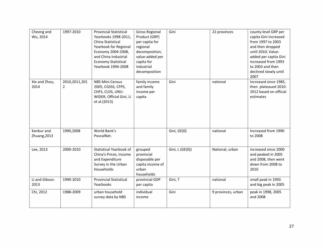
process in 1978 has been a focus of interest among analysts and policy makers. Table A gives a flavor of

this interest by summarizing the most significant studies concentrating on the evolution of income

inequality. In their study of the evolution of inequality in China focusing on spatial inequality over the

long run, from 1952 to 2000, Kanbur and Zhang (2005) identified two phases of inequality change after

the start of reforms in 1978. After an initial and short phase of falling inequality as rural incomes rose in

the wake of the liberalizations of the personal responsibility system, inequality rose inexorably as China

opened out to the world and explosive growth took place in the coastal regions.

This increase in inequality became an integral part of the narrative on Chinese development1, with

some commentators arguing that this was the inevitable price to be paid for the high rates of growth,

with others warning of the social consequences of rising gaps. In any event, “harmonious society” was

given center stage at the 2005 National People’s Congress and among rising policy concerns on

inequality. As more data has accumulated, greater attention has turned to an examination of the

evolution of inequality in China in the 2000s, including in the present decade--the years after 2010. A

number of studies which used data from the mid-2000s onwards began to argue that the rise in

inequality was being mitigated, and inequality was possibly plateauing and perhaps even turning down.2

This paper attempts to provide a comprehensive assessment of what the data show, a deeper look

into the patterns of inequality change, and preliminary explanations for the trends observed. Our basic

conclusion is that there does indeed appear to be a turnaround taking place in Chinese inequality, and

that the explanations lie in policy changes and in the nature of structural transformation in China.

The plan of the paper is as follows. Section 2 sets out the data sources on Chinese inequality on

which any assessment will have to be based. Section 3 then presents the basic trends over a twenty-year

period from 1995 to 2014. Section 4 examines the patterns of inequality change by looking, respectively,

1 See for example, Appleton, Song and Xia (2014); Chi, Li and Yu (2009); Chi (2012); Goh, Luo and Zhu (2009); Kanbur and Zhuang (2013); Knight (2014); Knight, Li and Wan (2016); Mendoza (2016). 2 Khan and Riskin (2005); Fan, Kanbur and Zhang (2011); Li et.al. (2016); Alvaredo et.al (2017); Chan et.al (2011); Li and Gibson (2013); Lee (2013); Cheong and Wu (2014); Zhang (2015); Xie and Zhou (2014); Xie et al. (2015). Even in Alvaredo et.al (2017), whose argument is that China’s inequality is approaching the US and is higher than France, the data shows that in China the top 1% share and the bottom 50% share have been plateauing since 2006. After 2010, the 1% share declined slightly and the bottom 50% share went up a little. In his review Knight (2014), focused on an earlier literature, asked, but did not substantiate, whether inequality had peaked. In Xie and Zhou (2014), the Gini coefficient estimated from various data sources show a plateauing trend from 2010 to 2012 except for the CHFS 2011, which drives the trend to be increasing as an outlier.

5

at decomposition by income source and by population subgroup. Section 5 presents some preliminary

explanation for the observed trends. Section 6 concludes.

2. Data

In this study, we use two kinds of data, household level data from household surveys and

provincial level data from the National Bureau of Statistics. Household level data are from two surveys,

Chinese Household Income Project (CHIP) and China Family Panel Studies (CFPS). CHIP was carried out as

part of a collaborative research project on incomes and inequality in China organized by Chinese and

international researchers including Institute of Economics of the Chinese Academy of Social Sciences and

School of Economics and Business at Beijing Normal University, with assistance from the National

Bureau of Statistics (NBS). There are six waves of cross-sectional data of CHIP, 1988, 1995, 2002, 2007,

2008, and 2013. China Family Panel Studies (CFPS) is a nationally representative, longitudinal survey

conducted every two years of Chinese communities, families, and individuals launched in 2010 by the

Institute of Social Science Survey (ISSS) of Peking University, China. It covers such topics as economic

activities, education outcomes, family dynamics and relationships, migration, and health. Currently,

there are three waves of panel data of CFPS, 2010, 2012 and 2014. Our provincial level income per

capita and population data is drawn from the National Bureau of Statistics database and multiple

provincial statistical year books.

We use household survey data to analyze household income inequality evolution and the

attributes from different income sources since it has rich information about different income

components in each household. As for the analysis of regional inequality evolution and its

decomposition, we make use of the provincial level data. Each data set is described below in greater

detail.

The household level data we use covers CHIP 1995, CHIP 2002, and CHIP 2007 (NBS sample),

CFPS 2010, CFPS 2012 and CFPS 2014. We did not go back to as early as 1988 because at that time, most

places in China were still under a command economy so that the income components in the 1988 survey

were quite different conceptually from those in the surveys later. CHIP 2007 and CHIP 2008 are also part

of the larger RUMiC (Rural-Urban Migrants in China) survey project. While the public RUMiC part data has a

different questionnaire from previous waves of CHIP and has no income component details, CHIP 2007 has a

restricted national representative NBS sample data, which is consistent with the previous waves. For this

reason, we drop CHIP 2008 in our analysis and use only the NBS sample from CHIP 2007. The detailed

questions about income details included in each wave between 1995 and 2007 of the CHIP data are quite

6

consistent. For CFPS, there are a few differences between CFPS 2010, CFPS2012 and CFPS2014. However,

adjusted incomes were provided in CFPS 2012 and CFPS 2014 to make them comparable with CFPS

20103.

There are some differences between CHIP and CFPS in the items included in each income

source4. For example, rental value of housing equity is included in CHIP 1995 but not in other surveys

and medical expenses paid by collective or government is included in transfer income in CHIP but not in

CFPS, etc. For the purpose of ensuring consistency as much as possible, we broke down the different

sources of income in CHIP and reconstructed them with the items that are included in CFPS only. In

addition, there is no “other income” in CHIP 2007, but we constructed it following CFPS’s definition.

Eventually, in our decomposition by income sources, we present two results, one with the original

household income from CHIP and CFPS, the other with adjusted income from CHIP which is consistent

with CFPS definition.

Another issue we need to address is the missing data in income sources. We assume that there

exists a fixed hidden distribution for household income, for both rural and urban categories. We

approximate the hidden distribution for rural and urban categories from the existing non-missing data.

Then we sample new pseudo value from this approximated distribution to fill the missing entries. The

pseudo value is a random number drawn from the sample distribution. This approximation for

distribution requires sufficiently large sample size which is a condition not satisfied using county level

sample. Provincial distribution is not suitable either since the CFPS is not representative on the province

level. Hence we use the national distribution.

In addition to the two issues addressed above, there are some observations for which the sum of

each income component does not equal the household net income in CFPS. This is due to the fact that

for households who did not report their annual net income, the household net income is estimated

according to their consumption. To deal with this issue, we rescale each income source using the

proportion household net incomesum of all the income sources

.

Although the two household surveys have rich information about household income, they have

different geographical coverage. Moreover, CFPS’s sampling are not representative on the provincial

level. Because of these limitations, we could not apply regional decomposition to the household survey

3 For details of the income component adjustment of CFPS, see Xie, Zhang, Xu and Zhang (2015). 4 For comparison of the two surveys, see Zhang, Xu, Zhou, Zhang and Xie (2014).

7

data. Therefore, in our analysis of regional inequality, the provincial level income and population data

from the NBS is used.

As Li and Gibson (2013) have noted, previously Chinese yearbooks regularly reported provincial

population and per capita economic outputs based on households registered, i.e. the Hukou population,

but not residential population. This resulted in a distortion of the estimate of provincial per capita

statistics in previous research papers. This distortion grew bigger as migrant workers increased since the

1990s. Recently, the NBS updated the provincial consumption per capita data based on residential

population for all provinces from 1993 to 2014. We also obtain population based on residential status

from both NBS and various Provincial Year Books 2011 and 2005, in which years, many provinces

updated their historical population data based on residence. The fact that the starting year of reporting

residential based population is different across provinces brings both disadvantages and advantages to

our study. On the one hand, the new NBS data is still not perfect though much improved than before.

On the other hand, on the aggregate level, there should not be systematic distortion as there does not

exist a cut-off year in which the statistical approach changed for all.

This is the data base for our assessment of Chinese inequality trends in the last twenty years. We

proceed now to a description of the overall trends and the decomposition patterns in the data.

3. Trends

We estimate various inequality measures using household survey data from CHIP and CFPS for

six points of time covering the twenty-year period between 1995 and 2014. Table 1 presents the Gini

coefficient and general entropy indices and Table 2 presents income ratios. The CHIP results in Panel A

of each table use original income per capita and those in panel B use adjusted income per capita to keep

consistent with CFPS. For both income construction methods, we see that the Gini coefficient has an

inverted U shape pattern with the turning point at 0.533 in 2010. The general entropy indices show

similar trends. For GE(0), the peak appears in 2012 while for GE(1) and GE(2) it is in 2010. The difference

of the turning pattern of each index could be a result of the fact that each inequality index captures

different characteristics of inequality. For the generalized entropy indices GE(c), the greater c is, the

more sensitive it is to the top income groups. That is to say, GE(0) is more sensitive to bottom income

groups while GE(2) is more sensitive to the top income groups.

8

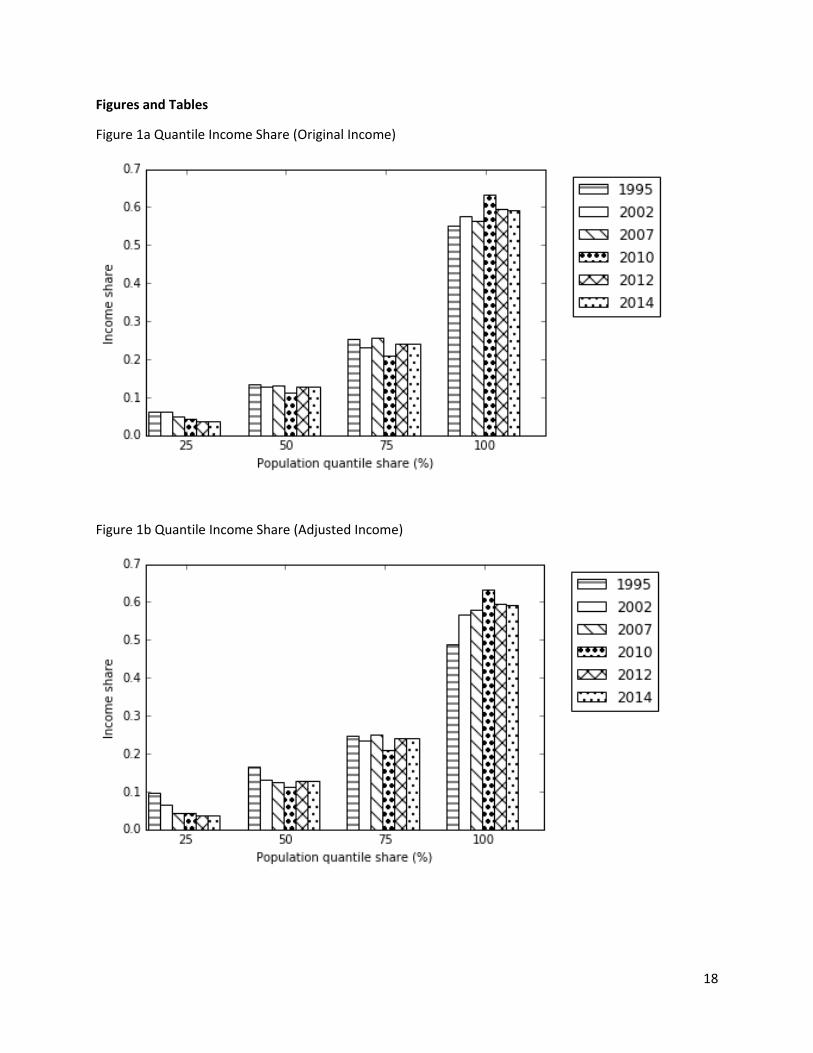
To have a more detailed picture of income distribution, quantile and decile income shares are

presented in Figure 1a, 1b, 2a and 2b. The income share of the top group reached the highest point in

2010, which is above 0.4 for the top 10% and above 0.6 for the top 25%, and then declined ever since.

2010 is also the year when the share of the middle group is the lowest. The narrowing inequality

measured by Gini coefficient, GE(1) and GE(2) since 2010 could be attributed to the rising middle group

income share and falling top group income share. While the top group’s income share had not been

increasing, the bottom group’s share seemed to worsen. We notice that income share of the very

bottom (25% in Figure 1a, 1b and 10% in Figure 2a, 3b) went down over the years which could increase

income inequality. As a matter of fact, the top-bottom income ratio went up from 1995 to 2012 and

declined a little afterwards. As shown in Table 2, the 90-10 ratio was as high as 19.87 in 2012 and then

fell to 19.12 in 2014. Meanwhile, the bottom-middle income ratio behaves like a U shape with a small

jump in 2010 and reached its lowest point in 2012. The 10-50 ratio fell from 0.259 in 2010 to 0.143 in

2012 and the 25-50 ratio fell from 0.516 in 2010 to 0.451 in 2012. This trend is possibly captured by the

turning behavior of GE(0), which peaked in 2012.

The combination of CHIP and CFPS data give us six observations spanning 1995 to 2014, based

on household surveys. An alternative data perspective, useful for capturing long term annual trends,

was introduced in Kanbur and Zhang (1999, 2005). This method uses NBS data on provincial

consumption per capita broken down by rural and urban for each province. Combining this with rural-

urban population data for each province (see the discussion on population data in Section 2), we can

construct a synthetic national consumption distribution which suppresses inequality within rural areas

and urban areas of each province. Clearly, this is an understatement of the level of inequality, but the

trend over time may nevertheless convey information on the evolution of inequality.

Column 1 of Table 11 presents the Gini coefficient over time for the synthetic distribution so

constructed, while Column 2 presents values for the GE(1), or Theil’s T, measure of inequality, for every

year from 1978 to 2014. The movements of the regional Gini coefficients and Theil’s T index are plotted

in Figure 3. The patterns of the two indices are quite similar. They went down a little after 1978 and

started to climb up slowly after 1985. In 1996, the regional inequality fell a little and showed a climbing

trend until 2004. Of course the values of the Gini and GE(1) in Table 11 are not comparable to the

corresponding values in Tables 1 and 2—income is used in one and consumption in another, within rural

and within-urban inequality is suppressed in one and not in the other, and the data sources are quite

different. However, the broad trends after the mid-1990s are similar from the two very different

9

perspectives—there appears to be an inequality turn around sometime towards the end of the first

decade of the 2000s.

Overall, then, a careful assessment of the best data sources seems to suggest a plateauing of

inequality, with a possible turning point around or just before 2010. To begin building an explanation of

the trend, we consider decomposition of inequality, first by income source and then by population

subgroup.

4. Decompositions

To unpack the patterns of inequality change, we proceed to decompose inequality, first by

income source, and then by population subgroup. To understand the role of different income sources in

the evolution of overall inequality, we decompose the Gini coefficient by income source following

Lerman and Yitzhaki’s (1985) rule.

G = ∑ 𝑆𝑆𝑘𝑘 ∑2

𝑛𝑛2𝜇𝜇𝑘𝑘�𝑖𝑖 − 𝑛𝑛+1

2�𝑌𝑌𝑘𝑘𝑘𝑘 = ∑ 𝑆𝑆𝑘𝑘�̅�𝐺𝑘𝑘 = ∑ 𝑆𝑆𝑘𝑘𝑅𝑅𝑘𝑘𝐺𝐺𝑘𝑘𝑘𝑘 𝑘𝑘𝑘𝑘𝑘𝑘 (1)

where Sk = 𝜇𝜇𝑘𝑘/𝜇𝜇 is the share of kth income component in total income, 𝐺𝐺𝑘𝑘���� is the “pseudo Gini”5, Rk is

the Gini correlation of component k with total income, and Gk is the Gini of income component k. The

absolute contribution of income source k to total income inequality is

vk(𝐺𝐺) = 𝑆𝑆𝑘𝑘𝑅𝑅𝑘𝑘𝐺𝐺𝑘𝑘 (2)

Its proportion of the total inequality is

𝑣𝑣�𝑘𝑘(𝐺𝐺) = 𝑆𝑆𝑘𝑘𝑅𝑅𝑘𝑘𝐺𝐺𝑘𝑘𝐺𝐺

=∑ �𝑘𝑘−𝑛𝑛+12 �𝑌𝑌𝑘𝑘𝑘𝑘𝑘𝑘

∑ �𝑘𝑘−𝑛𝑛+12 �𝑌𝑌𝑘𝑘𝑘𝑘 (3)

where Yi is the income of household i and Yki is the income from source k of household i6.

The marginal effect of income source k is

ηk(𝐺𝐺) = 𝑆𝑆𝑘𝑘(𝐺𝐺𝑘𝑘����𝐺𝐺− 1) (4)

5 The pseudo Gini is different from the conventional Gini since the weight attached to Yki corresponds to the rank of individual i in the total income distribution which is, in general, not the same as her rank in the distribution of income source k. 6 We weighted household income by family size in all calculations.

10

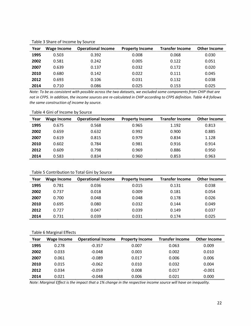
Table 3 shows the income share of each income source and Table 4 presents the Gini

coefficients of each income source. Wage income takes the largest share while its Gini coefficient is the

smallest. The share of property income has always been small, which is less than 10 percent, while its

Gini coefficient has been very high and stayed above 0.96. The proportionate contribution to total Gini

coefficient of each income source 𝑣𝑣�𝑘𝑘(𝐺𝐺) and their marginal effects ηk(𝐺𝐺) are reported in Table 5 and 6

respectively. The largest contribution is from wage income, which ranged between 0.7 and 0.8 over the

years, followed by transfer income, which ranged between 0.13 and 0.19. The contribution of other

incomes are lower than 0.1. In addition to the high contribution to overall Gini coefficient, wage income

also has the largest marginal effect.

Given the importance of wage income, the trends shown in Table 4 are central in understanding

the forces underlying the overall inequality trend. Inequality of wage income has fallen sharply, as has

inequality of transfers. These are the dominant factors in total income, and so their declining inequality

is the dominant factor in inequality change and accounts for the fall in inequality.

To see the sensitivity of the results, we also follow Paul (2004)’s extension on the Gini

decomposition to decompose Theil’s T index7, i.e. GE(1), by income sources.

T = ∑ ∑ 1𝑛𝑛𝜇𝜇

ln (𝑌𝑌𝑘𝑘𝜇𝜇

)𝑌𝑌𝑘𝑘𝑘𝑘𝑘𝑘𝑘𝑘 (5)

where µ is the mean of population income.

The absolute contribution to income inequality of income source k is

vk(𝑇𝑇) = ∑ (𝑙𝑙𝑙𝑙𝑌𝑌𝑘𝑘 − 𝑙𝑙𝑙𝑙𝜇𝜇)𝑌𝑌𝑘𝑘𝑘𝑘 𝑘𝑘 (6)

When expressed as a proportion of total inequality, it can be written as

𝑣𝑣�𝑘𝑘(𝑇𝑇) = vk(𝑇𝑇)/𝑇𝑇 = (∑ (𝑙𝑙𝑙𝑙𝑌𝑌𝑘𝑘 − 𝑙𝑙𝑙𝑙𝜇𝜇)𝑌𝑌𝑘𝑘𝑘𝑘)/ ∑ (𝑙𝑙𝑙𝑙𝑌𝑌𝑘𝑘 − 𝑙𝑙𝑙𝑙𝜇𝜇)𝑌𝑌𝑘𝑘 𝑘𝑘 𝑘𝑘 (7)

The marginal effect of income source k on Theil’s T index is

ηk(𝑇𝑇) = 1𝑇𝑇𝜇𝜇𝑛𝑛

∑ 𝑌𝑌𝑘𝑘(𝑆𝑆𝑘𝑘𝑘𝑘 − 𝑆𝑆𝑘𝑘)𝑙𝑙𝑙𝑙𝑌𝑌𝑘𝑘𝑘𝑘 (8)

7 We choose to decompose Theil’s T index here because for the general entropy class inequality measures GE(c), only when 0<c<2, the negativity requirement is met as shown in Paul (2004).

11

where Ski is the share of income source k in the total income of i-th household. The decomposition

results for Theil’s T index is presented in Table 7 and 8. The results are quite consistent with what we

find in the Gini decomposition.

In addition to the level of inequality, the over time change of inequality can also be expressed as

a weighted average of over time changes in each income source as stated in Paul et.al. (2012).

Define 𝐺𝐺𝑡𝑡,𝑡𝑡+1̇ = (𝐺𝐺𝑡𝑡+1 − 𝐺𝐺𝑡𝑡)/𝐺𝐺𝑡𝑡, which is the proportionate change in household income inequality

between year t and year t+1. It could be written as

�̇�𝐺𝑡𝑡,𝑡𝑡+1 = ∑ 𝑣𝑣�𝑘𝑘𝑘𝑘 (𝐺𝐺𝑡𝑡)�̇�𝑣𝑘𝑘(𝐺𝐺𝑡𝑡,𝑡𝑡+1) (9)

where 𝑣𝑣�𝑘𝑘(𝐺𝐺𝑡𝑡) serves as a weight, and �̇�𝑣𝑘𝑘�𝐺𝐺𝑡𝑡,𝑡𝑡+1� = 𝑣𝑣𝑘𝑘(𝐺𝐺𝑡𝑡+1)−𝑣𝑣𝑘𝑘(𝐺𝐺𝑡𝑡)𝑣𝑣𝑘𝑘(𝐺𝐺𝑡𝑡)

. Then the contribution of income

source k to the change of Gini coefficient is 𝑣𝑣 �𝑘𝑘(𝐺𝐺𝑡𝑡)�̇�𝑣𝑘𝑘(𝐺𝐺𝑡𝑡,𝑡𝑡+1). Similarly, the contribution of income

source k to the change of the Theil’s T index is 𝑣𝑣 �𝑘𝑘(𝑇𝑇𝑡𝑡)�̇�𝑣𝑘𝑘�𝑇𝑇𝑡𝑡,𝑡𝑡+1�.

The results for decomposition of the change of inequality are presented in Table 9 and 10. The

greatest contribution of the proportionate increase from 1995 to 2012 of the Gini coefficient and the

Theil’s T index were both from wage income, followed by transfer income. And from 2002 to 2007,

property income and operational income were the top two drivers for the proportionate increase of Gini

and the Theil’s T index. Wage income became the most important contributor to the dynamic change of

inequality again in the period between 2007 and 2010 for both inequality measures. When inequality

started to turn down from 2010 to 2012, operational income played the most important role. Later from

2012 to 2014, the contribution to the proportionate change of the Gini coefficient from wage income,

operational income and property income are quite close to each other. However for the Theil’s T index,

wage income served as the top inequality reducing component.

Overall, then, these accounting exercises are consistent with the hypothesis that it is the

narrowing of the wage distribution and the role of transfers which is important in beginning an

understanding of the Chinese inequality turnaround.

An alternative perspective on patterns of inequality change is through decomposition by

population subgroup. Unequal income distribution between urban and rural sectors is a feature in

developing countries for which China is not an exception. Besides the unequal development between

rural and urban regions, the disparity between the coastal areas in the east and inland areas in the

middle and west is also enormous (Fan, Kanbur and Zhang, 2011). To understand these components of

12

inequality, we use the data underlying Table 11, the synthetic distribution constructed from rural and

urban per capita consumption and population.

We further decompose the Theil’s T index by rural-urban subgroups and coastal-inland

subgroups respectively as in equation (10).

T = Tw + Tb = ∑ �𝑁𝑁𝑘𝑘𝑁𝑁�𝑘𝑘𝜇𝜇𝑘𝑘𝜇𝜇𝑇𝑇𝑘𝑘 + ∑ 𝑁𝑁𝑘𝑘

𝑁𝑁𝑘𝑘𝜇𝜇𝑘𝑘𝜇𝜇

ln �𝜇𝜇𝑘𝑘𝜇𝜇� = ∑ 𝑌𝑌𝑘𝑘

𝑌𝑌𝑘𝑘 𝑇𝑇𝑘𝑘 + ∑ 𝑌𝑌𝑘𝑘𝑌𝑌𝑘𝑘 ln �𝑌𝑌𝑘𝑘

𝑌𝑌/𝑁𝑁𝑘𝑘𝑁𝑁� (10)

where N is the total number of individuals and k is an indicator for groups, for example, rural or urban.

The first term is the within-group component of the Theil’s T index and the second term is the between-

group component.

The rural-urban between component and the coastal-inland between component are reported

in Table 11 and graphed in Figure 4. There are three peaks for the rural-urban between component in

1995, 2000 and 2004 respectively. After the third peak, the rural-urban between component kept a

declining trend. Notice that 2005 is the year when regional inequality and rural-urban between

components turned down. That is the year when, it has been argued, China passed the Lewis Turning

Point (Zhang, Yang and Wang, 2011). That is also the year when the agriculture tax was abolished and

the New Countryside Project was initiated. The coastal-inland between component fell in 2001 after a

high peak in 2000, then jumped again in 2005. It stayed at a relatively high level until 2009 and showed a

steady decline after that, contributing to the narrative of tightening labor markets in inland provinces,

and government policy to encourage development in the western regions. These explanations are taken

up in the next section.

5. Preliminary Explanations

Our main task in this paper has been to establish the key trends in Chinese inequality over the past

twenty years. Based on a number of perspectives, it does seem as though there was a turnaround in

Chinese inequality about 10 years ago, with inequality plateauing and even declining after a long period

of sharp increase. Explanations for this evolution will have to await detailed investigation from

researchers focusing on a range of factors in depth. However, in this section we present a broad

framework for such explanations.

13

A simple way to think of the evolution of national income distribution is to divide the economy up

into key sectors and to look at inequality within and between sectors. Given the importance of the

structural transformation which is underway in China just now we can begin our discussion in terms of

two sectors—rural and urban. The national income distribution is a weighted sum of the rural income

distribution and the urban income distribution, the weights being the population shares of the two

sectors. Overall inequality will then depend on (i) the inequality within each of the two sectors, (ii) the

gap between the means of the two sectoral distributions and (iii) the population share of each sector.

As an illustration, for the GE(0) index, also known as the mean log deviation, denoted L, the national

inequality can be decomposed as follows:

L = x L1 + (1-x) L2 + log [x k + (1-x)] – [x log (k)] (11)

where subscripts 1 and 2 denote rural and urban respectively, x is the population share of the urban

sector, and k is the ratio of the urban mean to the rural mean. The evolution of national inequality is

then composed of (i) the evolution of L1 and L2 (ii) the evolution of k and (iii) evolution of x.

With this framework, we can relate the inequality turnaround to basic economic forces and to

policy. First, as Zhang, Yang and Wang (2011) have argued, China has now reached the “Lewis turning

point”, where rural to urban migration begins to tighten rural labor markets and hereby mitigate the

rural-urban wage differential. In addition, heavy government investment in infrastructure in the rural

sector and in lagging regions, a feature of Chinese policy from the 2000s onwards (Fan, Kanbur and

Zhang, 2011), will also raise economic activity and incomes in these areas. This will surely lower k in (11)

and hence, ceteris paribus, overall inequality. This is consistent with the evolution of the rural-urban

component of inequality shown in Table 11, and it is further consistent with the observed reduction of

inequality in the national wage distribution as shown in Table 4.

The narrowing of the wage distribution and the increasing equality of the transfer distribution

shown in Table 4 can also be associated with policy changes. For example, in 2004 the Ministry of Labor

and Social Security issued a “Minimum Wage Regulations” law and the next decade saw rising minimum

wage standards coupled with substantial improvements in compliance (Kanbur, Li and Lin, 2016).

Further, a number of social programs were introduced and strengthened from the 2000s onwards. Since

2004 China has introduced new rural cooperative medical insurance, currently covering more than 95%

of rural population. Rural social security has also been rolled out since 2009. Although the premiums of

14

the rural medical insurance and social security are still much lower than the urban counterparts, the

programs have provided some cushions to rural residents against health risk and elderly care. A

combination of tightening labor markets in rural areas, and inequality mitigating transfer and regulation

regimes in urban and rural areas, acted through (i) and (ii) to reduce inequality.

The impact of x on L as seen through (11) is quite complex. Other factors constant, it can be

shown (Kanbur and Zhuang, 2013) that under certain conditions the behavior of L as a function of x has

an inverse-U shape as hypothesized by Kuznets (1955). Up to a certain point, urbanization increases

inequality, and beyond this point further urbanization will decrease inequality. This “Kuznets turning

point” sets out the effect of urbanization pure and simple on inequality. The turning point itself depends

on the other inequality parameters, but it is shown by Kanbur and Zhuang (2013) that Chinese

urbanization has now crossed the Kuznets turning point—further urbanization will reduce inequality

through channel (iii) above.

Of course each of these potential explanations needs to be investigated more fully and in

greater depth. But they appear to us to be consistent with underlying economic and policy forces which

can explain the inequality turnaround we see in the data.

6. Conclusion

We have argued in this paper that the long period of inequality increase in China is coming to an

end. The data, seen from different perspectives, seem to indicate a turnaround towards the latter part

of the 2010s. The explanations for this turnaround need to be explored further, but there is prima facie

evidence for economic forces and government policy tightening labor markets in rural areas, together

with government transfer and social policy mitigating inequality in urban and rural areas, which may

explain the observed trends. This of course raises the further question of why government policy

changed over a twenty-year period from allowing inequality to increase to mitigating it. The political

economy of the Chinese state (Wong, 2005) may provide an explanation, but that takes us beyond our

present remit.

15

References

Alvaredo, F, Chancel, L, Piketty, T, Saez, E, and Zucman, G, (2017)."Global Inequality Dynamics: New Findings from WID.world.'' National Bureau of Economic Research Working Paper 23119.

Appleton, S, Song, S and Xia, Q. (2014). “Understanding Urban Wage Inequality in China 1988 – 2008 : Evidence from Quantile Analysis.” World Development 62. 1-13.

Chan, K.S, Zhou, X and Pan, Z. (2014). “The Growth and Inequality Nexus : The Case of China ” International Review of Economics and Finance 34. 230-234.

Chen, Z, and Ge, Y. (2011). “Foreign Direct Investment and Wage Inequality : Evidence from China.” World Development 39 (8). 1322–32.

Cheng, Y, and Li, S. (2006). “Income Inequality and Efficiency : A Decomposition Approach and Applications to China” Economic Letters 91. 8–14

Cheong, T.S, and Wu Y. (2014). “The Impacts of Structural Transformation and Industrial Upgrading on Regional Inequality in China.” China Economic Review 31. 339–350.

Chi, W. (2012). “Capital Income and Income Inequality : Evidence from Urban China.” Journal of Comparative Economics 40 (2012). 228–39.

Chi, W, Li,B, and Yu, Q. (2011). “Decomposition of the Increase in Earnings Inequality in Urban China : A Distributional Approach ” China Economic Review 22: 299–312.

Démurger, S, Fournier,M, and Li, S. (2006). “Urban Income Inequality in China Revisited ( 1988 – 2002 )” Economics Letters 93: 354–359.

Fan, S, Kanbur, R, and Zhang, X. (2011). “China’s Regional Disparities: Experience and Policy.” Review of Development Finance 2011 (1): 47–56.

Fleisher, B, Li, H, and Zhao, M.Q. (2010). “Human Capital , Economic Growth , and Regional Inequality in China .” Journal of Development Economics 92: 215–231.

Gibson, J, and Li, C. (2015). “The Erroneous Use of China ’ S Population and per Capita Data : A Structured Review and Critical Test.” University of Waikato Department of Economics Working Paper.

Goh, C, Luo, X, and Zhu, N. (2009). “China Economic Review Income Growth , Inequality and Poverty Reduction : A Case Study of Eight Provinces in China.” China Economic Review 20: 485–496.

Kanbur, R and Zhang, X. (2005). “Fifty Years of Regional Inequality in China: A Journey Through Central Planning, Reform, and Openness ". Review of Development Economics, 9(1): 87–106.

Kanbur, R and Zhuang, J. (2013). “Urbanization and Inequality in Asia” Asian Development Review, vol. 30, no. 1: 131–147.

Khan, A.R and Riskin, Carl (2005).“China’s Household Income and Its Distribution, 1995 and 2002.” The China Quarterly, 182, June.

Knight, J. (2014). "Inequality in China: An Overview." World Bank Resrach Observer, 29 (1): 1-19.

Knight, J, Li, S, and Wan, H. (2016). “The Increasing Inequality of Wealth in China, 2002-2013 ". Department of Economics Discussion Paper Series (Ref: 816 ), University of Oxford.

16

Lee, J. (2013). “A Provincial Perspective on Income Inequality in Urban China and the Role of Property and Business Income.” China Economic Review 26: 140–150.

Li, C, and Gibson, J. (2013). “Rising Regional Inequality in China: Fact or Artifact?” World Development 47: 16–29.

Li, T, Lai, J.T, Wang, Y and Zhao. D. (2016). “Long-Run Relationship between Inequality and Growth in Post-Reform China : New Evidence from Dynamic Panel Model.” International Review of Economics and Finance 41: 238–52.

Mendoza, O M.V. (2016). “China Economic Review Preferential Policies and Income Inequality : Evidence from Special Economic Zones and Open Cities in China.” China Economic Review 40: 228–240.

Meng, X, Gregory, R and Wang, Y. (2005). “Poverty , Inequality , and Growth in Urban China ,” Journal of Comparative Economics 33: 710–729.

Meng, X, Shen, K, and Xue S. (2013). “Economic Reform , Education Expansion , and Earnings Inequality for Urban Males in China , 1988 – 2009.” Journal of Comparative Economics 41: 227–44.

Paul, S. (2004). “Income Sources Effects on Inequality.” Journal of Development Economics 73 (1): 435–451.

Paul, S, Chen, Z and Lu, M. (2012). “Household Income Structure and Rising Inequality in Urban China.” Working Paper, August 2012: 1–42.

Ravallion, M, and Chen, S. (2007). “China ’ S ( Uneven ) Progress against Poverty .” Journal of Development Economics 82: 1–42.

Shen, Y and Yao, Y. (2008). “Does Grassroots Democracy Reduce Income Inequality in China ? ” Journal of Public Economics 92: 2182–2198

Wan, G, Lu,M, and Chen, Z. (2006). “The Inequality – Growth Nexus in the Short and Long Run : Empirical Evidence from China.” Journal of Comparative Economics 34: 654–67.

Wang, Z, Smyth, R, and Ng, Y. (2009). “A New Ordered Family of Lorenz Curves with an Application to Measuring Income Inequality and Poverty in Rural China.” China Economic Review 20: 218–235.

Wong, R. Bin. (2011). “Social Spending in Contemporary China: Historical Priorities and Contemporary Possibilities,” In History, Historian, and Development Policy, edited by C.A. Bayly et al., 117-21. Manchester: Manchester University Press.

Xie, Y, Zhang, X, Xu, Q and Zhang C. (2015). "Short-term trends in China’s income inequality and poverty: evidence from a longitudinal household survey", China Economic Journa 8(3):1-17.

Xie, Y, and Zhou, X. (2014) “Income inequality in today’s China”. Proceedings of the National Academy of Sciences of the United States of America 111.19 (2014): 6928-2933.

Zhang, C, Xu, Q, Zhou, X, Zhang, X, and Xie, Y. (2014) "Are poverty rates underestimated in China? New evidence from four recent surveys". China Ecnomic Review 31： 410-425

Zhang, C. (2015). “Income Inequality and Access to Housing : Evidence from China ” China Economic Review 36: 261-271

Zhang, X. (2006). “Fiscal Decentralization and Political Centralization in China : Implications for Growth

17

and Inequality.” Journal of Comparative Economics 34: 713–26.

Zhang, X, Yang, J, and Wang, S. (2011). "China has reached the Lewis turning point." China Economic Review, 22(4): 542-554

18

Figures and Tables

Figure 1a Quantile Income Share (Original Income)

Figure 1b Quantile Income Share (Adjusted Income)

19

Figure 2a Decile Income Share (Original Income)

Figure 2b Decile Income Share (Adjusted Income)

20

Table 1 Inequality Measures from Household Survey Data A: Original income Year Data Gini GE(0) GE(1) GE(2) 1995 CHIP 0.435 0.347 0.320 0.420 2002 CHIP 0.458 0.369 0.359 0.486 2007 CHIP 0.459 0.409 0.359 0.459 2010 CFPS 0.533 0.551 0.571 1.389 2012 CFPS 0.504 0.590 0.496 1.319 2014 CFPS 0.495 0.566 0.456 0.915

B: Adjusted income Year Data Gini GE(0) GE(1) GE(2) 1995 CHIP 0.349 0.206 0.215 0.300 2002 CHIP 0.445 0.344 0.340 0.466 2007 CHIP 0.478 0.446 0.400 0.601 2010 CFPS 0.533 0.551 0.571 1.389 2012 CFPS 0.504 0.590 0.496 1.319 2014 CFPS 0.495 0.566 0.456 0.915

Note1: Panel A uses the original income from each survey. Panel B adjusted CHIP income by excluding the components that are not in CFPS.CHIP 2007 uses the NBS survey data, not RUMiC survey since the latter uses a different questionnaire and sample framework while the former is consistent with previous years.

21

Table 2 Income Ratio from Household Survey Data A: Original income Year Data p90_p10 p75_p25 p90_p50 p75_p50 p10_p50 p25_p50 1995 CHIP 8.719 3.489 2.876 1.880 0.330 0.539 2002 CHIP 9.109 3.450 3.265 1.954 0.358 0.566 2007 CHIP 11.968 3.980 2.815 1.805 0.235 0.453 2010 CFPS 13.361 3.660 3.466 1.888 0.259 0.516 2012 CFPS 19.873 3.895 2.846 1.755 0.143 0.451 2014 CFPS 19.122 3.854 2.920 1.765 0.153 0.458

B: Adjusted income Year Data p90_p10 p75_p25 p90_p50 p75_p50 p10_p50 p25_p50 1995 CHIP 4.820 2.262 2.266 1.532 0.470 0.677 2002 CHIP 8.319 3.296 3.099 1.907 0.372 0.579 2007 CHIP 13.192 4.269 2.945 1.849 0.223 0.433 2010 CFPS 13.361 3.660 3.466 1.888 0.259 0.516 2012 CFPS 19.873 3.895 2.846 1.755 0.143 0.451 2014 CFPS 19.122 3.854 2.920 1.765 0.153 0.458

Note1: Panel A uses the original income from each survey. Panel B adjusted CHIP income by excluding the components that are not in CFPS.Note2: CHIP 2007 uses the NBS survey data, not RUMiC survey since the latter uses a different questionnaire and sample framework while the former is consistent with previous years.

22

Table 3 Share of Income by Source Year Wage Income Operational Income Property Income Transfer Income Other Income 1995 0.503 0.392 0.008 0.068 0.030 2002 0.581 0.242 0.005 0.122 0.051 2007 0.639 0.137 0.032 0.172 0.020 2010 0.680 0.142 0.022 0.111 0.045 2012 0.693 0.106 0.031 0.132 0.038 2014 0.710 0.086 0.025 0.153 0.025

Note: To be as consistent with possible across the two datasets, we excluded some components from CHIP that are not in CFPS. In addition, the income sources are re-calculated in CHIP according to CFPS definition. Table 4-8 follows the same construction of income by source.

Table 4 Gini of Income by Source Year Wage Income Operational Income Property Income Transfer Income Other Income 1995 0.675 0.568 0.965 1.192 0.813 2002 0.659 0.632 0.992 0.900 0.885 2007 0.619 0.815 0.979 0.834 1.128 2010 0.602 0.784 0.981 0.916 0.914 2012 0.609 0.798 0.969 0.886 0.950 2014 0.583 0.834 0.960 0.853 0.963

Table 5 Contribution to Total Gini by Source Year Wage Income Operational Income Property Income Transfer Income Other Income 1995 0.781 0.036 0.015 0.131 0.038 2002 0.737 0.018 0.009 0.181 0.054 2007 0.700 0.048 0.048 0.178 0.026 2010 0.695 0.080 0.032 0.144 0.049 2012 0.727 0.047 0.039 0.149 0.037 2014 0.731 0.039 0.031 0.174 0.025

Table 6 Marginal Effects Year Wage Income Operational Income Property Income Transfer Income Other Income 1995 0.278 -0.357 0.007 0.063 0.009 2002 0.033 -0.048 0.003 0.002 0.010 2007 0.061 -0.089 0.017 0.006 0.006 2010 0.015 -0.062 0.010 0.032 0.004 2012 0.034 -0.059 0.008 0.017 -0.001 2014 0.021 -0.048 0.006 0.021 0.000

Note: Marginal Effect is the impact that a 1% change in the respective income source will have on inequality.

23

Table 7 Contribution to Theil’s T by Source Year Wage Income Operational Income Property Income Transfer Income Other Income 1995 1.013 -0.247 0.024 0.163 0.046 2002 0.887 -0.200 0.014 0.233 0.065 2007 0.720 -0.026 0.113 0.161 0.033 2010 0.664 0.078 0.062 0.143 0.052 2012 0.779 0.000 0.048 0.137 0.034 2014 0.770 -0.008 0.038 0.174 0.026

Table 8 Marginal Effects Year Wage Income Operational Income Property Income Transfer Income Other Income 1995 0.511 -0.442 0.017 0.095 0.016 2002 0.307 -0.163 0.009 0.112 0.015 2007 0.081 -0.063 0.081 -0.011 0.012 2010 -0.015 -0.105 0.040 0.032 0.007 2012 0.086 -0.094 0.018 0.005 -0.003 2014 0.060 -0.094 0.013 0.021 0.001

Table 9 Contribution to The Change of Gini Coefficient by Source (%) Year Change Wage Income Operational Income Property Income Transfer Income Other Income

1995-2002 27.3 15.8 -1.2 -0.4 10.0 3.0 2002-2007 7.5 1.5 3.3 4.3 1.0 -2.5 2007-2010 11.6 7.6 4.1 -1.2 -1.8 2.8 2010-2012 -5.6 -0.9 -3.6 0.4 -0.3 -1.4 2012-2014 -1.7 -0.8 -0.9 -0.9 2.2 -1.2

Table 10 Contribution to The Change of Theil’s T by Source (%) Year Change Wage Income Operational Income Property Income Transfer Income Other Income

1995-2002 57.6 38.5 -6.9 -0.2 20.5 5.6 2002-2007 17.8 -3.9 17.0 11.8 -4.4 -2.7 2007-2010 42.7 22.9 13.7 -2.4 4.4 4.1 2010-2012 -13.2 1.2 -7.8 -2.0 -2.4 -2.2 2012-2014 -8.1 -7.1 -0.8 -1.4 2.3 -1.0

24

Table 11 Regional Inequality and Between Components Year Gini GE(1) (Theil’s T) Rural-Urban Coastal-Inland 1978 0.281 0.162 14.657 0.250 1979 0.273 0.149 13.144 0.258 1980 0.268 0.136 11.556 0.406 1981 0.258 0.120 9.835 0.484 1982 0.236 0.100 7.941 0.436 1983 0.226 0.090 6.920 0.468 1984 0.228 0.090 6.810 0.496 1985 0.236 0.098 7.283 0.538 1986 0.245 0.105 7.549 0.645 1987 0.253 0.113 7.907 0.717 1988 0.261 0.120 8.126 0.843 1989 0.266 0.123 7.703 0.888 1990 0.277 0.136 8.713 0.742 1991 0.282 0.140 9.242 0.547 1992 0.294 0.148 9.638 0.662 1993 0.307 0.164 10.689 0.819 1994 0.311 0.170 10.989 1.141 1995 0.324 0.181 12.037 1.762 1996 0.303 0.158 9.917 1.274 1997 0.308 0.163 10.369 1.341 1998 0.314 0.171 10.925 1.476 1999 0.328 0.186 11.931 1.508 2000 0.342 0.196 12.694 2.000 2001 0.337 0.188 11.618 1.282 2002 0.348 0.202 12.606 1.347 2003 0.354 0.208 13.530 1.358 2004 0.372 0.229 14.575 1.268 2005 0.364 0.213 13.957 2.306 2006 0.362 0.210 13.695 2.328 2007 0.363 0.210 13.619 2.293 2008 0.361 0.207 13.187 2.307 2009 0.357 0.202 12.923 2.400 2010 0.353 0.197 12.359 2.316 2011 0.354 0.199 11.516 2.276 2012 0.344 0.188 10.345 2.163 2013 0.338 0.182 9.548 2.197 2014 0.329 0.172 8.419 2.142

Note: Data is from NBS and various Provincial Statistical Year Books

25

26

Appendix

Table A: Summary of Studies on China’s Inequality Trends

Author & year Years covered Data source Income concept Inequality measure Population coverage

Trend of inequality established

Alvaredo et.al 2017

1978-2014 World Wealth and Income Database

Pre-tax national income

Top 1% income share and bottom 50% income share

national Increased a lot since 1978 and plateaued after 2006

Knight, Li, and Wan 2016

2002, 2013 CHIP household wealth and household income

Gini 21 in 2002 and 14 in 2013

Increased

Li et.al. 2016 1984-2012 Ravallion and Chen (2007) and NBS 2003-2012

income per capita

Gini, urban rural income ratio

27 provinces increased from 1984 to 1994, then decreased until 1997, then increased until 2005 and decreased afterwards

Mendoza Graduate, 2016

1988.1995.2002

CHIP household disposable income per capita

Gini 12-16 provinces increased from 1988 to 2002

Xie, Zhang, Xu and Zhang, 2015

2000, 2003-2012

CFPS, CGSS, CHFS, CHIP, NBS (from Xie, et al. 2013)

family income per capita

Gini 25 provinces plateaued since 2003 and declined from 2010 to 2012

Zhang, 2015 2002-2009 Chinese urban household survey by NBS

household disposable income per capita

Gini 186 cities in 16 provinces

peaked in 2005 and 2008, then went down a little in 2009

Appleton, Song and Xia, 2014

1988,1995, 2002,2008

CHIP household income per capita

Gini; General Entropy Index, Atkinson Index; income ratio

12-16 provinces, urban

sharp increases in inequality largely due to changes in the wage structure

27

Cheong and Wu, 2014

1997-2010 Provincial Statistical Yearbooks 1998-2011, China Statistical Yearbook for Regional Economy 2004-2008, and China Industrial Economy Statistical Yearbook 1994-2008

Gross Regional Product (GRP) per capita for regional decomposition, value-added per capita for industrial decomposition

Gini 22 provinces county level GRP per capita Gini increased from 1997 to 2003 and then dropped until 2010; Value-added per capita Gini increased from 1993 to 2003 and then declined slowly until 2007

Xie and Zhou, 2014

2010,2011,2012

NBS Mini-Census 2005, CGSSS, CFPS, CHFS, CLDS, UNU-WIDER, Official Gini, Li et al.(2013)

family income and family income per capita

Gini national Increased since 1985, then plateaued 2010-2012 based on official estimates

Kanbur and Zhuang,2013

1990,2008 World Bank’s PovcalNet.

Gini, GE(0) national Increased from 1990

to 2008

Lee, 2013 2000-2010 Statistical Yearbook of China's Prices, Income and Expenditure Survey in the Urban Households

grouped provincial disposable per capita income of urban households

Gini, L (GE(0)) National, urban increased since 2000 and peaked in 2005 and 2008, then went down from 2008 to 2010

Li and Gibson. 2013

1990-2010 Provincial Statistical Yearbooks

provincial GDP per capita

Gini, T national small peak in 1993 and big peak in 2005

Chi, 2012 1988-2009 urban household survey data by NBS

individual income

Gini 9 provinces, urban peak in 1998, 2005 and 2008

28

Chan, Zhou and Pan,2011

1995-2011 China Statistical Yearbook for Regional Economy

grouped income per person from each decile

average adjusted Gini 26 provinces big peak in 2002 and went down 2009-2011

Fan, Kanbur and Zhang, 2011

1952-2007 Comprehensive Statistical Data and Materials on 50 Years of New China, China Statistical Yearbook

provincial per capita consumption

Gini, GE(1) national peaks in 1960, 1975, 2005 and troughs in 1952, 1967

Chi, Li and Yu, 2009

1987,1996,2004

NBS urban household survey

total individual income

Gini, GE(1) national increasing

Goh, Luo and Zhu, 2009

1989, 2004 CHNS per capita household income

Gini 8 provinces increasing

Wang et al, 2009

1980,1985,1990, 1995-2006

China Rural Household Survey Yearbook

grouped average annual income per capita

Kakwani index, Chakravarty index, Gini

national peak in 2003 and reduced a little afterwards

Shen and Yao, 2008

1987-2002 National Fixed-point Survey (NFS)

household per-capita income

Gini national, rural relative steady before 1994, increased a lot after 1996, a trough in 1996 and a peak in 2001

Ravallion and Chen,2007

1980–2001 Rural Household Surveys (RHS) and the Urban Household Surveys (UHS) of NBS

tabulation of distribution of income per capita

Gini national decreasing 1980-1982, increasing 1982-1994, deceasing 1994-1996, increasing 1996-2001

Démurger, Fournier and Li, 2006

1988,1995,2002

CHIP household total disposable income

Gini, GE(1), GE(0) Urban increased 1988-1995, decreased 1995-2002

Khan and Riskin, 2005

1995, 2002 CASS survey of households

household per capita income

Gini 11 provinces in the urban sample and 19 provinces in the

Both rural and urban inequality decreased,

29

rural sample for 1995, 21 provinces in the rural sample for 2002

but the national inequality unchanged

Kanbur and Zhang, 2005

1952-2000 Statistical Year Books real per capita consumption in the rural and urban areas

Gini, GE(0) 28 provinces Peaks in 1960, 1976, troughs in 1967, 1984, increased 1984-2000

Meng et al, 2005

1986-2000 NBS Urban Household Income and Expenditure Survey (UHIES)

real income and real net expenditure

Gini national, urban increased

WP No Title Author(s)

OTHER A.E.M. WORKING PAPERS

Fee(if applicable)

A Supply Chain Impacts of Vegetable DemandGrowth: The Case of Cabbage in the U.S.

Yeh, D., Nishi, I. and Gómez, M.2017-05

A systems approach to carbon policy for fruitsupply chains: Carbon-tax, innovation instorage technologies or land-sparing?

Alkhannan, F., Lee, J., Gómez, M. andGao, H.

2017-04

An Evaluation of the Feedback Loops in thePoverty Focus of World Bank Operations

Fardoust, S., Kanbur, R., Luo, X., andSundberg, M.

2017-03

Secondary Towns and Poverty Reduction:Refocusing the Urbanization Agenda

Christiaensen, L. and Kanbur, R.2017-02

Structural Transformation and IncomeDistribution: Kuznets and Beyond

Kanbur, R.2017-01

Multiple Certifications and ConsumerPurchase Decisions: A Case Study ofWillingness to Pay for Coffee in Germany

Basu, A., Grote, U., Hicks, R. andStellmacher, T.

2016-17

Alternative Strategies to Manage WeatherRisk in Perennial Fruit Crop Production

Ho, S., Ifft, J., Rickard, B. and Turvey, C.2016-16

The Economic Impacts of Climate Change onAgriculture: Accounting for Time-invariantUnobservables in the Hedonic Approach

Ortiz-Bobea, A.2016-15

Demystifying RINs: A Partial EquilibriumModel of U.S. Biofuels Markets

Korting, C., Just, D.2016-14

Rural Wealth Creation Impacts of Urban-based Local Food System Initiatives: A DelphiMethod Examination of the Impacts onIntellectual Capital

Jablonski, B., Schmit, T., Minner, J., Kay,D.

2016-13

Parents, Children, and Luck: Equality ofOpportunity and Equality of Outcome

Kanbur, R.2016-12

Intra-Household Inequality and OverallInequality

Kanbur, R.2016-11

Anticipatory Signals of Changes in CornDemand

Verteramo Chiu, L., Tomek, W.2016-10

Capital Flows, Beliefs, and Capital Controls Rarytska, O., Tsyrennikov, V.2016-09

Paper copies are being replaced by electronic Portable Document Files (PDFs). To request PDFs of AEM publications, write to (be sure toinclude your e-mail address): Publications, Department of Applied Economics and Management, Warren Hall, Cornell University, Ithaca, NY14853-7801. If a fee is indicated, please include a check or money order made payable to Cornell University for the amount of yourpurchase. Visit our Web site (http://dyson.cornell.edu/research/wp.php) for a more complete list of recent bulletins.

WP No Title Author(s)

OTHER A.E.M. WORKING PAPERS

Fee(if applicable)

Inequality Indices as Tests of Fairness Kanbur, R. and Snell, A.2017-07

The Great Chinese Inequality Turn Around Kanbur, R., Wang, Y. and Zhang, X.2017-06

A Supply Chain Impacts of Vegetable DemandGrowth: The Case of Cabbage in the U.S.

Yeh, D., Nishi, I. and Gómez, M.2017-05

A systems approach to carbon policy for fruitsupply chains: Carbon-tax, innovation instorage technologies or land-sparing?

Alkhannan, F., Lee, J., Gómez, M. andGao, H.

2017-04

An Evaluation of the Feedback Loops in thePoverty Focus of World Bank Operations

Fardoust, S., Kanbur, R., Luo, X., andSundberg, M.

2017-03

Secondary Towns and Poverty Reduction:Refocusing the Urbanization Agenda

Christiaensen, L. and Kanbur, R.2017-02

Structural Transformation and IncomeDistribution: Kuznets and Beyond

Kanbur, R.2017-01

Multiple Certifications and ConsumerPurchase Decisions: A Case Study ofWillingness to Pay for Coffee in Germany

Basu, A., Grote, U., Hicks, R. andStellmacher, T.

2016-17

Alternative Strategies to Manage WeatherRisk in Perennial Fruit Crop Production

Ho, S., Ifft, J., Rickard, B. and Turvey, C.2016-16

The Economic Impacts of Climate Change onAgriculture: Accounting for Time-invariantUnobservables in the Hedonic Approach

Ortiz-Bobea, A.2016-15

Demystifying RINs: A Partial Equilibrium Modelof U.S. Biofuels Markets

Korting, C., Just, D.2016-14

Rural Wealth Creation Impacts of Urban-based Local Food System Initiatives: A DelphiMethod Examination of the Impacts onIntellectual Capital

Jablonski, B., Schmit, T., Minner, J., Kay,D.

2016-13

Parents, Children, and Luck: Equality ofOpportunity and Equality of Outcome

Kanbur, R.2016-12

Intra-Household Inequality and OverallInequality

Kanbur, R.2016-11

Paper copies are being replaced by electronic Portable Document Files (PDFs). To request PDFs of AEM publications, write to (be sure toinclude your e-mail address): Publications, Department of Applied Economics and Management, Warren Hall, Cornell University, Ithaca, NY14853-7801. If a fee is indicated, please include a check or money order made payable to Cornell University for the amount of yourpurchase. Visit our Web site (http://dyson.cornell.edu/research/wp.php) for a more complete list of recent bulletins.