Working Over Time: Dynamic Inconsistency in RealE↵ort Tasks ⇤

Ned Augenblick †

UC Berkeley, Haas School of Business

Muriel Niederle‡

Stanford University and NBER

Charles Sprenger§

Stanford University

First Draft: July 15, 2012This Version: January 15, 2013

Abstract

Experimental tests of dynamically inconsistent time preferences have largely relied onchoices over time-dated monetary rewards. Several recent studies have failed to find thestandard patterns of time inconsistency. However, such monetary studies contain often-discussed confounds. In this paper, we sidestep these confounds and investigate choicesover consumption (real e↵ort) in a longitudinal experiment. We pair those e↵ort choiceswith a companion monetary discounting study. We confirm very limited time inconsis-tency in monetary choices. However, subjects show considerably more present bias ine↵ort. Furthermore, present bias in the allocation of work has predictive power for de-mand of a meaningfully binding commitment device. Therefore our findings validate a keyimplication of models of dynamic inconsistency, with corresponding policy implications.

JEL classification: C91, D12, D81

Keywords : Time Discounting, Demand for Commitment, Real E↵ort, Convex Time Budget

⇤We are grateful for many helpful discussions including those of Ste↵en Andersen, James Andreoni, ColinCamerer, Yoram Halevy, David Laibson, Matthew Rabin, Georg Weizsacker and participants at the StanfordInstitute for Theoretical Economics. We thank Wei Wu for helpful research assistance and technological exper-tise.

†University of California Berkeley, Haas School of Business, University of California, Berkeley, 545 StudentServices Building, 1900, Berkeley, CA, 94720-1900. ned@haas.berkeley.edu

‡Stanford University, Department of Economics, Landau Economics Building, 579 Serra Mall, Stanford, CA94305; niederle@stanford.edu, www.stanford.edu/⇠niederle

§Stanford University, Department of Economics, Landau Economics Building, 579 Serra Mall, Stanford, CA94305; cspreng@stanford.edu.

1 Introduction

Models of dynamically inconsistent time preferences (Strotz, 1956; Laibson, 1997; O’Donoghue

and Rabin, 1999) are a pillar of modern behavioral economics, having added generally to

economists’ understanding of the tensions involved in consumption-savings choices, task per-

formance, temptation, and self-control beyond the standard model of exponential discounting

(Samuelson, 1937). Given the position of present-biased preferences in the behavioral litera-

ture, there is clear importance in testing the model’s central falsifiable hypothesis of diminishing

impatience through time. Further, testing auxiliary predictions such as individuals’ potential

to restrict future activities through commitment devices can deliver critical prescriptions to

policy makers. In this paper we present a test of dynamic inconsistency in consumption and

investigate the demand for a meaningfully binding commitment device.

To date, a notably large body of laboratory research has been generated focused on identify-

ing the shape of time preferences (for a comprehensive review to the early 2000s, see Frederick,

Loewenstein and O’Donoghue, 2002).1 The core of this experimental literature has identified

preferences from time-dated monetary payments. A paradigmatic example would have a sub-

ject state the monetary payment received today, $X, that makes her indi↵erent to $50 received

in one months’ time, then would have her state the monetary payment received in one months’

time, $Y , that makes her indi↵erent to $50 received in two months’ time.2 Non-equivalence in

the stated indi↵erent values is often taken as evidence of dynamic inconsistency, and $X < $Y is

taken as evidence of a present-biased shape of discounting. Though conducted experiments dif-

fer along many dimensions including payment horizons, methods, subject pools, and potential

1Though much of the literature has focused on laboratory samples, there is also a growing body of researchattempting to identify the shape and extent of discounting from real world choices and aggregate data such asdurable goods purchase, annuity choice, and consumption patterns (Hausman, 1979; Lawrance, 1991; Warnerand Pleeter, 2001; Gourinchas and Parker, 2002; Cagetti, 2003; Laibson, Repetto and Tobacman, 2003, 2005).

2A popular methodolgy for eliciting such indi↵erences is the Multiple Price List technique (Coller andWilliams, 1999; Harrison, Lau and Williams, 2002) asking individuals a series of binary choices between timedated payments, identifying intervals in which $X and $Y lie. Psychology has often relied on an alternativemethod to identify dynamic inconsistency, asking subjects a series of questions involving increasing delay lengthsand examining whether the implied discount factors nest exponentially (see, for example Kirby, Petry and Bickel,1999; Giordano, Bickel, Loewenstein, Jacobs, Marsch and Badger, 2002).

2

transaction costs, a stylized fact has emerged that many subjects are dynamically inconsistent

and the majority of inconsistencies are in the direction of present bias (Frederick et al., 2002).3

Several confounds exist for identifying the shape of time preferences from experimental

choices over time-dated monetary payments, muddying the strict interpretations of behavior

provided above. Critically, issues of payment reliability and risk preference suggest that if in-

formation is to be gleaned from such choices, it may be linked to the subject’s assessment of

the experimenter’s reliability.4 Recent work validates this suspicion. Andreoni and Sprenger

(2012a), Gine, Goldberg, Silverman and Yang (2010), and Andersen, Harrison, Lau and Rut-

strom (2012) all document that when closely controlling transactions costs and payment re-

liability, dynamic inconsistency in choices over monetary payments is virtually eliminated on

aggregate. Further, when payment risk is added in an experimentally controlled way, non-

expected utility risk preferences deliver behavior observationally equivalent to present bias as

described above (Andreoni and Sprenger, 2012b).5

Beyond these operational issues, there is reason to question the use of potentially fungible

monetary payments to identify the parameters of models defined over time-dated consump-

tion. Clear arbitrage arguments exist indicating that nothing beyond the interval of subjects’

borrowing and lending rates should be revealed in choices over monetary payments.6 Chabris,

3For example, Ashraf, Karlan and Yin (2006) find that roughly 47% of their subjects are dynamicallyinconsistent over hypothetical time-dated monetary payments and around 60% of the inconsistencies are inthe direction of present bias. Similarly, Meier and Sprenger (2010) find that roughly 45% of their subjectsare dynamically inconsistent over incentivized time dated payments and 80% of the inconsistencies are in thedirection of present bias.

4This point was originally raised by Thaler (1981) who, when considering the possibility of using incentivizedmonetary payments in intertemporal choice experiments noted ‘Real money experiments would be interestingbut seem to present enormous tactical problems. (Would subjects believe they would get paid in five years?)’

5Specifically, Andreoni and Sprenger (2012b) show that when sooner payments are certain while future pay-ments are delivered only with 80%, subjects prefer the certain sooner payment. When payments at both timeperiods are made uncertain, occurring with 50% sooner and 40% in the future, subjects appear more patient,violating discounted expected utility. The observation that non-expected utility risk preferences generate dy-namic inconsistencies was previously thoughtfully analyzed theoretically by Machina (1989). Halevy (2008)makes the link between prospect theory probability weighting and diminishing impatience through time citingpsychology experiments conducted by Keren and Roelofsma (1995) and Weber and Chapman (2005) who showin an original experiment and a partial reproduction, respectively, that when payment risk is added to binarychoices over monetary payments, dynamic inconsistency is reduced in some experimental contexts.

6This point has been thoughtfully taken into account in some studies. For example, Harrison et al. (2002)explicitly account for potential arbitrage in their calculations of individual discount rates by measuring individualborrowing and saving rates and incorporating these values in estimation. Cubitt and Read (2007) provide

3

Laibson and Schuldt (2008) describe the di�culty in mapping experimental choices over money

to corresponding model parameters, casting skepticism over monetary experiments in general.

The model is one of consumption, so falsifying the key prediction of diminishing impatience

through time may be more convincing when done in the relevant domain, consumption.7 There

are only a few experimental tests of dynamic inconsistency for consumption. Key contributions

include Read and van Leeuwen (1998) who identify dynamic inconsistency in the surprise real-

locations of snack choices, and McClure, Laibson, Loewenstein and Cohen (2007) and Brown,

Chua and Camerer (2009), who document dynamic inconsistency in brief intertemporal choices

over squirts of juice and soda.

In this paper we attempt to move out of the domain of monetary choices and into the

domain of consumption, while maintaining a portable design that allows individual parameters

of dynamic inconsistency to be estimated. With 102 UC Berkeley Xlab subjects, we introduce

a seven week longitudinal experimental design asking subjects to allocate and subsequently

reallocate units of e↵ort (i.e., negative leisure consumption) over time at various gross interest

rates. Subject responses are incentivized by requiring completion of the tasks from either

one initial allocation or one subsequent reallocation. Subjects receive a one-time completion

bonus of $100 in the seventh week of the experiment, fixing the monetary dimension of their

e↵ort allocation choices. The tasks over which subjects make choices are transcription of

meaningless greek texts and completion of partial tetris games. Allocations are made in a

convex decision environment permitting identification of both cost function and discounting

parameters. Di↵erences between initial allocations and subsequent reallocations allow for the

identification of dynamic inconsistency.

The repeated interaction of our seven-week study allows us to complement measures of e↵ort

excellent recent discussion of the arbitrage arguments and other issues for choices over monetary payments.One counterpoint is provided by Coller and Williams (1999), who present experimental subjects with a fullyarticulated arbitrage argument and external interest rate information and document only a small treatmente↵ect.

7Though our objective in the present study is the exploration of present bias separate from issues of fungibility,recent developments in the field have led to another important facet of the debate: why and when do monetarydiscounting studies deliver measures of present bias with predictive validity despite their potential flaws? Thisquestion lies outside the scope of this paper but clearly represents an important avenue for future research.

4

discounting with measures of monetary discounting taken from Andreoni and Sprenger (2012a)

Convex Time Budget (CTB) choices over cash payments received in the laboratory. In these

choices, subjects allocate money across time at various gross interest rates. We can compare

dynamic inconsistency measured over work and money at both the aggregate and individual

level.

Finally, once subjects have experienced the tasks for several weeks, we elicit their demand

for a commitment device. Specifically, we allow subjects to probabilistically favor their initial

allocations over their subsequent reallocations of work. We investigate the aggregate demand

for our o↵ered commitment device and correlate identified dynamic inconsistency over both

e↵ort and money with commitment demand.

We document three primary findings. First, in the domain of money we find virtually

no aggregate evidence of present bias using immediate in-lab cash payments. Second, in the

domain of e↵ort we find significant evidence of present bias. Allocations of tasks made one

week in advance exceed those made on the date of actual e↵ort by approximately 9%, on

average. Corresponding parameter estimates corroborate these non-parametric results. Third,

we find that the elicited demand for commitment is limited to price zero, at which price 59%

of subjects would prefer a higher likelihood of implementing one of their initial allocations

over their subsequent reallocations. More importantly, we show that subjects we identified as

present biased choose the commitment device, while others do not. We show that the choice

of commitment is binding and meaningful in the sense that initial preferred allocations di↵er

significantly from subsequent reallocations. This provides key validation and support for our

experimental measures and well-known theoretical models of present bias.

Despite recent negative findings for models of dynamic inconsistency with time-dated pay-

ments, we find support for the model’s central prediction of diminishing impatience through

time in the domain of consumption. Further, the auxiliary predictions of both the potential

demand for commitment and the link between commitment demand and present bias are also

validated.

5

The paper proceeds as follows: Section 2 provides details for our longitudinal experimental

design. Section 3 describes identification of intertemporal parameters based on experimental

choices over both e↵ort and money. Section 4 presents results. Section 5 is a discussion and

section 6 concludes.

2 Design

To examine dynamic inconsistency in real e↵ort, we introduce a longitudinal experimental

design conducted over seven weeks. In the experiment, subjects are asked to allocate, sub-

sequently reallocate and complete tasks for two jobs. If all elements of the experiment are

completed satisfactorily, subjects receive a completion bonus of $100 in Week 7 of the study.

Otherwise they receive only $10 in Week 7. The objective of the completion bonus is to fix the

monetary dimension of subjects’ e↵ort choices. Subjects are always paid the same amount for

their completed work, the question of interest is when they prefer to exert e↵ort.

Having individuals make intertemporal choices over e↵ort allows us to circumvent many of

the key concerns that plague monetary discounting experiments. First, subjects cannot borrow,

save or substitute units of tasks outside of the experiment, removing opportunities of arbitrage.8

Second, the precise date of consumption is known to both the researcher and the subject at the

time of decision, allowing for precise identification of discounting parameters. Third, individuals

select into a seven week experiment with a $100 completion bonus in the seventh week, reducing

issues of payment reliability. This also separates e↵ort allocation decisions from payment. And

lastly, we implement a minimum work requirement. This equalizes transaction costs over time

as subjects are forced to participate and complete minimum e↵ort on all dates.

We present the design in five subsections. First, we describe the Jobs to be completed.

Second, we present a timeline of the experiment and the convex decision environment in which

allocations were made. The third subsection describes the design of the commitment device

8Though this removes substitutability of the task at hand, subjects may alter their allocations of other,extra-lab consumption. As a first pass we ignore this possibility and the possibility that subjects subcontracttheir experimental tasks. Section 6 provides additional discussion.

6

for which demand was elicited once subjects had gained experience with the tasks. The fourth

subsection addresses design details including recruitment, selection and attrition. The fifth

subsection presents the complementary monetary discounting study facilitated by the repeated

interaction with subjects during the experiment.

2.1 Jobs

The experiment focuses on intertemporal allocations of e↵ort. Subjects are asked to allocate,

subsequently reallocate and complete tasks of two jobs. In Job 1, subjects transcribe a mean-

ingless greek text through a computer interface. Figure 1, Panel A demonstrates the paradigm.

Greek letters appear in random order, slightly blurry, in subjects’ transcription box. By point-

ing and clicking on the corresponding keyboard below the transcription box, subjects must

reproduce the observed series of Greek letters. One task is the completion of one row of Greek

text with 80 percent accuracy as measured by the Levenshtein Distance.9 In the first week,

subjects completed a task from Job 1 in an average of 54 seconds. By the final week, the

average was 46 seconds.

In Job 2, subjects are asked to complete four rows of a standard tetris game. Figure 1,

Panel B demonstrates the paradigm. Blocks of random shapes appear at the top of the tetris

box and fall at fixed speed. Arranging the shapes to complete a horizontal line of the tetris

box is the game’s objective. Once a row is complete, it disappears and the shapes above fall

into place. One task is the completion of four rows of tetris. If the tetris box fills to the top

with shapes before the four rows are complete, the subject begins again with credit for the rows

already completed. In the first week, subjects completed a task from Job 2 in an average of 55

seconds. By the final week, the average was 46 seconds.

9The Levenshtein Distance is commonly used in computer science to measure the distance between twostrings and is defined as the minimum number of edits needed to transform one string into the other. Allowableedits are insertion, deletion or change of a single character. As the strings of Greek characters used in thetranscription task are 35 characters long our 80 percent accuracy measure is equivalent to 7 edits or less or aLevenshtein Distance 7.

7

Figure 1: Experimental Jobs

Panel A: Job 1- Greek Transcription

Panel B: Job 2- Partial Tetris Games

2.2 Experimental Timeline and Allocation Environment

2.2.1 Timeline

The seven weeks of the experiment are divided into two blocks. Weeks 1, 2, and 3 serve as

the first block. Weeks 4, 5, and 6 serve as the second block and mirror the first block with

the addition of a commitment decision discussed below. Week 7 occurs in the laboratory and

is only used to distribute payment to the subjects. Subjects always participate on the same

8

day of the week throughout the experiment. That is, subjects entering the lab on a Monday

allocate tasks to be completed on future Mondays. Therefore, the time frame over which e↵ort

choices are made is exactly seven days in all choices.

Weeks 1 and 4 occur in the laboratory and subjects are reminded of their study time the

night before. Weeks 2, 3, 5, and 6 are completed online. For Weeks 2, 3, 5, and 6, subjects

are sent an email reminder at 8pm the night before with a (subject-unique) website address.

Subjects are required to log in to this website between 8am and midnight of the day in question

and complete their work by 2am the following morning.

At each point of contact, subjects are first given instructions about the decisions to be

made and work to be completed that day, reminded of the timeline of the experiment, given

demonstrations of any unfamiliar actions, and then asked to complete the necessary actions.

In each week, subjects are required to complete 10 tasks of each Job prior to making

allocations decision or completing allocated tasks. The objective of this pair of 10 tasks,

which we call “minimum work,” is two-fold. First, minimum work requires a few minutes of

participation at each date, forcing subjects to incur the transaction costs of logging on to the

experimental website at each time.10 Second, minimum work, especially in Week 1, provides

experience for subjects such that they have a sense of how e↵ortful the tasks are when making

their allocation decisions. We require minimum work in all weeks before all decisions and

provide this information to subjects to control for issues related to projection bias (Loewenstein,

O’Donoghue and Rabin, 2003). This ensures that subjects have experienced and can forecast

having experienced the same amount of e↵ort when making their allocation decisions at all

points in time.

10A similar technique is used in monetary discounting studies where minimum payments are employed toeliminate subjects loading allocations to certain dates to avoid transaction costs of receiving multiple paymentsor cashing multiple checks (Andreoni and Sprenger, 2012a).

9

2.2.2 Allocation Environment

In Week 1, subjects allocate tasks between Weeks 2 and 3. Hence, subjects are choosing how

much work to complete at two future dates. In Week 2, subjects also allocate tasks between

Weeks 2 and 3. Note that in Week 1 subjects are making decision involving two future dates,

whereas in Week 2, subjects are making decisions involving the present and a future date.

Before making the choice in Week 1, subjects are told of the Week 2 decisions and are aware

that exactly one of all Week 1 and Week 2 allocation decisions will be implemented.11

Initial allocations and subsequent reallocations for Jobs 1 and 2 are made in a convex

decision environment. Using slider bars, subjects allocate tasks to two dates, one earlier and

one later, under di↵erent gross interest rates.12 Figure 2 provides a sample allocation screen.

To motivate the intertemporal tradeo↵s faced by subjects, decisions are described as having

di↵erent ‘task rates’ such that every task allocated to the sooner date reduces the number of

tasks allocated to the later date by a stated number. For example, a task rate of 1:0.5 implies

that each task allocated to Week 2 reduces by 0.5 the number allocated to Week 3. It is

important to note that the minimum 10 tasks required for each job detailed in the previous

section are separate from this allocation decision and are not counted toward the allocations.

The subjects’ decision can be formulated as allocating tasks e over times t and t+ k, et and

et+k, subject to the present-value budget constraint,

et +1

p· et+k = m, (1)

where 1/p represents the provided task rate. For each task and for each date where allocations

were made, subjects faced five task rates, 1/p 2 {0.5, 0.75, 1, 1.25, 1.5}. The number of tasks

that subjects could allocate to the sooner date was fixed at fifty such that m = 50 in every

decision in the experiment. Note that as the task rate falls, the relative cost of a task in Week

11Subjects were not shown their initial allocations when making their subsequent reallocations.12Passive allocations are avoided in the design as the sliders’ initial location was in the middle of the slider

bar and subjects were required to click on every slider before submitting their answers.

10

2 (the earlier week) falls, altering intertemporal incentives.

Figure 2: Convex Allocation Environment

In Weeks 1 and 2 each subject makes 20 allocation decisions: five for each Job in Week

1 and five for each Job in Week 2. After the Week 2 decisions, one of these 20 allocations is

chosen at random as the ‘allocation-that-counts’ and subjects have to complete the allocated

number of tasks to ensure successful completion of the experiment. However, the random-

ization device probabilistically favors the Week 2 allocations over the Week 1 allocations. In

particular, subjects are told (from the beginning) that their Week 1 allocations will count with

probability 0.1, while their Week 2 reallocations will count with probability 0.9. Within each

week’s allocations, every choice is equally likely to be the allocation-that-counts.13 This ran-

domization process e↵ectively favors flexibility while maintaining incentive compatibility in a

comprehensible manner. This design choice was made for two reasons. First, it increased the

chance that subjects experienced their own potentially present-biased reallocations. Second,

it provides a greater symmetry to the decisions in the second block of three weeks that elicit

demand for commitment.13For a complete description of the randomization process please see instructions in Appendix C.

11

The second block of the experiment, Weeks 4, 5, and 6, mimics the first block of Weeks 1, 2,

and 3, with one exception. In Week 4, subjects are o↵ered a probabilistic commitment device,

which is described in detail in the following subsection.

2.3 Commitment Demand

In the second block of the experiment, Weeks 4, 5, and 6, once subjects have gained experience

with the tasks and the experimental design, they are o↵ered a probabilistic commitment de-

vice. In the first block of the experiment, the allocation-that-counts is taken from the Week 1

allocations with probability 0.1 and from the subsequent Week 2 reallocations with probability

0.9, favoring the later reallocations. In Week 4, subjects are given the opportunity to choose

which allocations will be probabilistically favored. In particular, they can choose whether the

allocation-that-counts comes from Week 4 with probability 0.1 (and Week 5 with probability

0.9), favoring flexibility, or from Week 4 with probability 0.9, favoring commitment. This form

of commitment device was chosen because of its potential to be meaningfully binding. Sub-

jects who choose to commit and who di↵er in their allocation choices through time can find

themselves constrained by commitment with high probability.

In order to operationalize our elicitation of commitment demand, subjects are asked to

make 15 multiple price list decisions between two options. In the first option, the allocation-

that-counts will come from Week 4 with probability 0.1. In the second option, the allocation-

that-counts will come from Week 4 with probability 0.9. In order to determine the strength

of preference, an additional payment of between $0 and $10 is added to one of the options for

each decision.14 Figure 3 provides the implemented price list. One of the 15 commitment

decisions is chosen for implementation, ensuring incentive compatibility. Subjects are told that

the implementation of the randomization for the commitment decisions will occur once they

submitted their Week 5 allocation decisions.

Our commitment demand decisions, and the second block of the experiment, serve three

14We chose not to have the listed prices ever take negative values (as in a cost) to avoid subjects viewingpaying for commitment as a loss.

12

Figure 3: Commitment Demand Elicitation

purposes. First, they allow us to assess the demand for commitment and its extent. If indi-

viduals demand commitment, it is important to know both how much they are willing to pay

for the opportunity to restrict their future activities and to help separate commitment demand

from simple decision error. Second, a key objective of our study is to explore the theoretical

link, under the assumption of sophistication, between present bias and commitment demand.

Are subjects who are present biased comparing initial allocations to subsequent reallocations

more likely to demand commitment? With the exception of Ashraf et al. (2006) and Kaur,

Kremer and Mullainathan (2010) virtually no research tests this critical implication of models

of dynamic inconsistency. We will compare our results to those papers in subsection 4.4. Fi-

nally, a correlation between time inconsistency and commitment validates the interpretation of

present bias over other explanations for time inconsistent e↵ort choices.

To summarize our longitudinal e↵ort experiment, Table 1 contains the major events in each

week.

13

Table 1: Summary of Longitudinal Experiment

Minimum 10 E↵ort Allocation-That- Complete Commitment ReceiveWork Allocations Counts Chosen Work Choice Payment

Week 1 (In Lab): x xWeek 2 (Online): x x x xWeek 3 (Online): x xWeek 4 (In Lab): x x xWeek 5 (Online): x x x xWeek 6 (Online): x xWeek 7 (In Lab): x

2.4 Design Details

102 subjects from the UC Berkeley Xlab subject pool were initially recruited into the experiment

across 4 experimental sessions on February 8th, 9th and 10th, 2012 and were told in advance

of the seven week longitudinal design and the $100 completion bonus.15 Subjects did not

receive an independent show up fee. 90 subjects completed all aspects of the working over time

experiment and received the $100 completion bonus. The 12 subjects who selected out of the

experiment do not appear di↵erent on either initial allocations, comprehension or a small series

of demographic data collected at the end of the first day of the experiment.16 One more subject

completed initial allocations in Week 1, but due to computer error did not have their choices

recorded. This leaves us with 89 subjects.

One critical aspect of behavior limits our ability to make inference for time preferences

based on experimental responses. In particular, if subjects have no variation in allocations

in response to gross interest rate changes in some weeks, then attempting to point identify

both discounting and cost function parameters is di�cult or impossible, yielding imprecise and

unstable estimates. Similar to multiple price list experiments, if a subject always chooses a

15This is a potentially important avenue of selection into the experiment. Our subjects were willing to putforth e↵ort and wait seven weeks to receive $100. Though we have no formal test, this suggests that our subjectsmay be a relatively patient selection.

163 of those 12 subjects dropped after the first week while the remaining 9 dropped after the second week.Including data for these 9 subjects where available does not qualitatively alter the analysis or conclusions.

14

specific option, only one-sided bounds on parameters can be obtained. Here, the problem is

compounded by our e↵orts to identify both discounting and cost function parameters. In our

sample, nine subjects have this issue for one or more weeks of the study. For the analysis, we

focus on the primary sample of 80 subjects who completed all aspects of the experiment with

positive variation in their responses in each week. In Appendix Table A2, we re-conduct the

aggregate analysis including these nine subjects and obtain very similar findings.

2.5 Monetary Discounting

Subjects were present in the UC Berkeley X-Laboratory in the first, fourth, and seventh weeks

of the experiment. This repeated interaction facilitates a monetary discounting study that

complements our main avenue of analysis. In Weeks 1 and 4 of our experimental design, once

subjects complete their allocation of tasks, they are invited to respond to additional questions

allocating monetary payments to Weeks 1, 4, and 7. In Week 1, we implement three Andreoni

and Sprenger (2012a) Convex Time Budget (CTB) choice sets, allocating payments across: 1)

Week 1 vs. Week 4; 2) Week 4 vs. Week 7 (Prospective); and 3) Week 1 vs. Week 7. Individuals

are asked to allocate monetary payments c across the two dates t and t+k, ct and ct+k, subject

to the intertemporal budget constraint,

r · ct + ct+k = m. (2)

The experimental budget is fixed at m = $20 and five gross interest rates are implemented in

each choice set, r 2 {0.99, 1, 1.11, 1.25, 1.43}. These gross interest rates were chosen for com-

parison with prior work (Andreoni and Sprenger, 2012a).17 Such questions permit identification

of monetary discounting parameters following Andreoni and Sprenger (2012a). In Week 4, we

ask subjects to allocate in a CTB choice set over Week 4 and Week 7 under the same five gross

interest rates. We refer to these choices made in Week 4 as Week 4 vs. Week 7 and those made

in Week 1 over these two dates as Week 4 vs. Week 7 (Prospective). Hence, subjects complete

17Additionally, r = 0.99 allows us to investigate the potential extent of negative discounting.

15

a total of four CTB choice sets.

The CTBs implemented in Weeks 1 and 4 are paid separately and independently from the

rest of the experiment with one choice from Week 1 and one choice from Week 4 chosen to be

implemented. Subjects are paid according to their choices. Subjects are not told of the Week

4 choices in Week 1. As in Andreoni and Sprenger (2012a), miniminum payments of $5 at each

payment date are enacted to eliminate transaction cost issues similar to those discussed above.

Appendix C provides the full experimental instructions.

The implemented monetary discounting experiments have two nuances relative to Andreoni

and Sprenger (2012a). First, Andreoni and Sprenger (2012a) implement CTBs with payment

by check. Our design implements payment by cash with potentially lower transaction costs.

Second, Andreoni and Sprenger (2012a) implement CTBs with present payment received only

by 5:00 p.m. in a subject’s residence mailbox. Here we provide payment immediately in the

laboratory limiting arguments about the relevant epoch of the present.

In both Weeks 1 and 4, the monetary allocations are implemented after the more central

e↵ort choices. The monetary choices were not announced in advance and subjects could choose

not to participate; five did so in either Weeks 1 or 4. In our analysis of monetary discounting,

we focus on the 75 subjects from the primary sample with complete monetary choice data.

3 Identification

In the intertemporal allocation of e↵ort and money, discounting and additional parameters can

be identified at either the aggregate or individual level under various structural assumptions. In

the following two subsections we describe which experimental variation provides identification

of specific parameters of interest and lay out methodology for estimation at both the aggregate

and individual level.

16

3.1 E↵ort Discounting

In the working over time experiment, subjects allocate e↵ort to an earlier date, et, and a later

date, et+k, subject to the intertemporal budget constraint described in (1). Hence, the subject’s

decision problem is

minet,et+kC(et, et+k) s.t. et +

1

pet+k = m,

where C(et, et+k) is a general cost function, assumed to be globally convex such that standard

constrained optimization yields meaningful first order conditions. We assume that the cost

function is time separable, that the instantaneous cost function is stationary and takes an

exponential form, and that discounting follows the quasi-hyperbolic form proposed by Laibson

(1997). Under these structural assumptions we can write

C(et, et+k) = (et + !)� + �1t=0�k(et+k + !)�, (3)

where � > 1 represents the stationary parameter on the convex instantaneous cost of e↵ort

function. The present-bias parameter, �, activated when the time period t is the present, 1t=0,

captures the extent to which individual’s disproportionately discount the future when viewed

from the present. The parameter � captures the daily discount factor over the k = 7 days of

each considered allocation. The additive term ! in the cost function could be interpreted as

a Stone-Geary minimum or as some background level of required work. Such parameters are

used in monetary discounting studies (Andersen, Harrison, Lau and Rutstrom, 2008; Andreoni

and Sprenger, 2012a), and are either taken from some external data source on background

consumption or estimated from experimental choices. For simplicity, we interpret ! as the

required minimum work of the experiment and set ! = 10.

Minimizing (3) subject to (1) yields the intertemporal Euler equation

(et + !

et+k + !)(��1)(

1

�(1t=0)�k) = p.

17

Rearranging and taking logs yields

log(et + !

et+k + !) =

log(�)

� � 1· (1t=0) +

log(�)

� � 1· k + (

1

� � 1) · log(p), (4)

which is linear in the key experimentally varied parameters of whether allocations involve the

present, 1t=0, and a log transform of the task rate, log(p).

From the intertemporal Euler equation above, identification of discounting and the cost

function is straightforward. The task rate delivers identification of the cost function, �; the

choice being made in the present (Week 2 decision) rather than the future (Week 1 decision)

delivers identification of present bias, �; and the delay length gives identification of the discount

factor, �.18

In order to estimate discounting and cost function parameters from aggregate data, we

assume an additive error structure and estimate the linear regression implied by (4). The

parameters of interest can be recovered from non-linear combinations of regression coe�cients

with standard errors calculated via the delta method.19 One important issue to consider in

the estimation of (4) is the potential presence of corner solutions. We provide estimates from

two-limit tobit regressions designed to account for the possibility that the tangency condition

implied by (4) does not hold with equality (Wooldridge, 2002).

Estimating (4) is easily extended to the study of individual parameters. To begin, (4) can

be estimated at the individual level.20 However, with limited numbers of individual choices

it is helpful to consider alternative, more structured approaches. In particular, we allow for

heterogeneous discounting across individuals, but assume all individuals have the same cost

18Of course, with only one delay length of seven days considered in the experiment, we have limited confidencethat our estimate of � can be extrapolated to arbitrary delay lengths.

19To be specific, the regression equation is, for k = 7,

log(et + !

et+k + !

)i = ⌘0k + ⌘1 · (1t=0)i + ⌘2 · log(p)i + ✏i,

and we recover the parameters of interest as �̂ = exp(⌘̂1/⌘̂2) and �̂ = 1 + 1/⌘̂2. Note that �̂ = exp(⌘̂0/⌘̂2) isrecovered from the constant as only one delay length was used in the experimental design.

20Broadly similar conclusions are reached when estimating (4) at the individual level, however, parameterprecision is greatly reduced and substantial estimate instability is uncovered in some cases.

18

function. Consider a vector of fixed e↵ects (1j)i which take the value 1 if observation i was

contributed by individual j. This leads to the fixed e↵ects formulation

log(et + !

et+k + !)i =

log(�)

� � 1· k +

(log(�j)� log(�))

� � 1· (1j)i · k +

log(�)

� � 1· (1t=0)i

+(log(�j)� log(�))

� � 1· (1t=0)i · (1j)i +

1

� � 1· log(p)i,

where �, � refer to sample means, and �j, �j refer to individual-specific discounting param-

eters. With an additive error structure this is easily estimable.21 The individual fixed e↵ect

interacted with the decision being made in the present provides identification of the individual-

specific �j. In Appendix A we conduct simulation exercises under various correlation structures

for the true parameters of interest and document that the implemented estimation methods

perform well both at the aggregate and individual level.

3.2 Monetary Discounting

Our methods for recovering monetary discounting parameters at both the aggregate and indi-

vidual level closely follow those for e↵ort. Following most of the literature, we abstract from

standard arbitrage arguments for monetary discounting and assume laboratory administered

rates are the relevant ones.22 In particular, for monetary payments, ct and ct+k, allocated

subject to the constraint (2), we assume a quasi-hyperbolic constant relative risk averse utility

function,

U(ct, ct+k) = (ct + !)↵ + �1t=0�k(ct+k + !)↵. (5)

Here, the utility function is assumed to be concave, ↵ < 1, such that first order conditions

provided meaningful optima. Here, the parameter ! is a background parameter that we take

21We allow both � and � to vary across individuals such that the implemented regression is a standardinteraction with both level and slope e↵ects.

22One prominent exception to this tradition is Harrison et al. (2002), who measure and account for extra-labborrowing and savings opportunities.

19

to be the $5 minimum payment of the monetary experiment.23

Maximizing (6) subject to the intertemporal budget constraint (2) yields an intertemporal

Euler equation similar to that above for e↵ort. Taking logs and rearranging we have

log(ct + !

ct+k + !) =

log(�)

↵� 1· (1t=0) +

log(�)

↵� 1· k + (

1

↵� 1) · log(r), (6)

which can again be estimated at the aggregate or individual level via two-limit Tobit. Discount-

ing and utility function parameters can be recovered via non-linear combinations of regression

coe�cients as above with standard errors estimated again via the delta method.

4 Results

The results are presented in three subsections. First, we present results from the monetary

discounting study and compare our observed level of limited present bias with other recent

findings. Second, we move to e↵ort related discounting and provide both non-parametric and

parametric evidence of present bias. In a third subsection we present results related to commit-

ment demand and document correlations between identified present bias over work and money

with the demand for our lab-o↵ered commitment device.

4.1 Monetary Discounting

Figure 4 presents the data from our monetary discounting experiment. The mean allocation

to the sooner payment date at each interest rate is reported for the 75 subjects from the

primary sample for whom we have all monetary discounting data. Four data series are provided

separated by delay length corresponding to the four payment sets over which subjects made

allocations. Standard error bars are provided, clustered at the individual level.

23Andreoni and Sprenger (2012a) provide detailed discussion of the use of such background parameters andprovide robustness tests with di↵ering values of ! and di↵ering assumptions for the functional form of utilityin CTB estimates. The findings suggest that though utility function curvature estimates may be sensitive todi↵erent background parameter assumptions, discounting parameters, particularly present bias, are virtuallyuna↵ected by such choices.

20

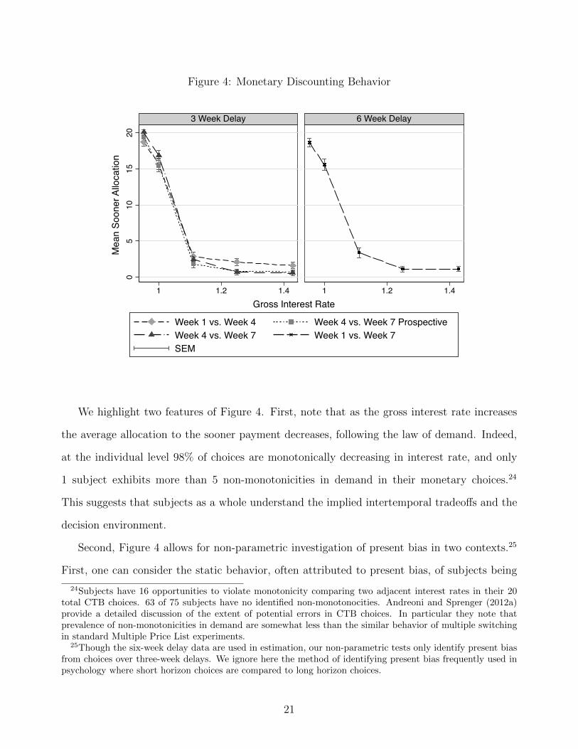
Figure 4: Monetary Discounting Behavior

05

1015

20

1 1.2 1.4 1 1.2 1.4

3 Week Delay 6 Week Delay

Week 1 vs. Week 4 Week 4 vs. Week 7 ProspectiveWeek 4 vs. Week 7 Week 1 vs. Week 7SEM

Mea

n So

oner

Allo

catio

n

Gross Interest Rate

Graphs by moneyk

We highlight two features of Figure 4. First, note that as the gross interest rate increases

the average allocation to the sooner payment decreases, following the law of demand. Indeed,

at the individual level 98% of choices are monotonically decreasing in interest rate, and only

1 subject exhibits more than 5 non-monotonicities in demand in their monetary choices.24

This suggests that subjects as a whole understand the implied intertemporal tradeo↵s and the

decision environment.

Second, Figure 4 allows for non-parametric investigation of present bias in two contexts.25

First, one can consider the static behavior, often attributed to present bias, of subjects being

24Subjects have 16 opportunities to violate monotonicity comparing two adjacent interest rates in their 20total CTB choices. 63 of 75 subjects have no identified non-monotonocities. Andreoni and Sprenger (2012a)provide a detailed discussion of the extent of potential errors in CTB choices. In particular they note thatprevalence of non-monotonicities in demand are somewhat less than the similar behavior of multiple switchingin standard Multiple Price List experiments.

25Though the six-week delay data are used in estimation, our non-parametric tests only identify present biasfrom choices over three-week delays. We ignore here the method of identifying present bias frequently used inpsychology where short horizon choices are compared to long horizon choices.

21

more patient in the future than in the present by comparing Week 1 vs. Week 4 to Week 4 vs.

Week 7 (Prospective). In this comparison, controlling for interest rate fixed e↵ects, subjects

do allocate on average $0.54 (s.e = 0.31) more to the sooner payment when it is in the present

F (1, 74) = 2.93, (p = 0.09). A second measure of present bias is to compare Week 4 vs. Week

7 (Prospective) made in Week 1 to the Week 4 vs. Week 7 choices made in Week 4. This

measure is similar to the recent work of Halevy (2012). Ignoring income e↵ects associated with

having potentially received prior experimental payments, this comparison provides a secondary

measure of present bias. In this comparison, controlling for interest rate fixed e↵ects, subjects

allocate on average $0.47 (s.e = 0.32) more to the sooner payment when the sooner payment

is in the present, F (1, 74) = 2.08, (p = 0.15).26

Over monetary payments, we find limited non-parametric support for the existence of a

present bias. In Table 2, columns (1) and (2) we provide corresponding parameter estimates

implementing two-limit Tobit regressions of (6), with standard errors clustered at the individual

level. In column (1) we use all 4 CTB choice sets. In column (2) we use only the choice sets

which have three-week delays for continuity with both our non-parametric evidence and the

comparisons generally made in experimental economics. In both cases we estimate ↵̂ of around

0.975 indicating limited utility function curvature over monetary payments. Further, we identify

daily discount factors of around 0.998. The 95% confidence interval in column (1) for the daily

discount factor implies annual discount rates between 40% and 140%.27

In column (1) of Table 2 we estimate �̂ = 0.974 (s.e. = 0.009), close to dynamic consistency.

Though we do reject the null hypothesis of � = 1, �2(1) = 8.77, (p < 0.01), our estimated

value for � is economically close to 1. In column (2), focusing only on three week delay data,

we find �̂ = 0.988 (0.009) and are unable to reject the null hypothesis of dynamic consistency,

26Additionally, this measure is close in spirit to our e↵ort experiment where initial allocations are comparedto subsequent reallocations. To get a sense of the size of potential income e↵ects, we can also compare theWeek 1 vs. Week 4 choices made in Week 1 to the Week 4 vs. Week 7 choices made in Week 4. Controlling forinterest rate fixed e↵ects, subjects allocate on average $0.07 (s.e = 0.31) more to the sooner payment in Week1, F (1, 74) = 0.05, (p = 0.82), suggesting negligible income e↵ects.

27Admittedly, our ability to precisely identify aggregate discounting was not a focus of the experimentaldesign and is compromised by limited variation in delay length and interest rates. In monetary discountingexperiments it is not unusual to find implied annual discount rates in excess of 100%.

22

Table 2: Parameter Estimates

Monetary Discounting E↵ort Discounting

(1) (2) (3) (4) (5)All Delay Three Week Delay Job 1 Job 2 CombinedLengths Lengths Greek Tetris

Present Bias Parameter: �̂ 0.974 0.988 0.900 0.877 0.888(0.009) (0.009) (0.037) (0.036) (0.033)

Daily Discount Factor: �̂ 0.998 0.997 0.999 1.001 1.000(0.000) (0.000) (0.004) (0.004) (0.004)

Monetary Curvature Parameter: ↵̂ 0.975 0.976(0.006) (0.005)

Cost of E↵ort Parameter: �̂ 1.624 1.557 1.589(0.114) (0.099) (0.104)

# Observations 1500 1125 800 800 1600# Clusters 75 75 80 80 80Job E↵ects Yes

H0 : � = 1 �2(1) = 8.77 �2(1) = 1.96 �2(1) = 7.36 �2(1) = 11.43 �2(1) = 11.42(p < 0.01) (p = 0.16) (p < 0.01) (p < 0.01) (p < 0.01)

H0 : �(Col. 1) = �(Col. 5) �2(1) = 6.37(p = 0.01)

H0 : �(Col. 2) = �(Col. 5) �2(1) = 8.26(p < 0.01)

Notes: Parameters identified from two-limit Tobit regressions of equations (6) and (4) formonetary discounting and e↵ort discounting, respectively. Parameters recovered via non-linearcombinations of regression coe�cients. Standard errors clustered at individual level reportedin parentheses, recovered via the delta method. E↵ort regressions control for Job E↵ects (Task1 vs. Task 2). We use Chi-squared tests for the null hypotheses in the last three rows.

�2(1) = 1.96, (p = 0.16). For a fixed delay length and interest rate, subjects make virtually

identical allocations in the present and the future.

Our non-parametric and parametric results closely mirror the aggregate findings of Andreoni

and Sprenger (2012a) and Gine et al. (2010).28 A potential concern of these earlier studies that

carefully control transaction costs and payment reliability, is that a payment in the present

was implemented by a payment in the afternoon of the same day, e.g. by 5:00 pm in the

subjects’ residence mailboxes in Andreoni and Sprenger (2012a). In this paper, because subjects

28In both of these prior exercises substantial heterogeneity in behavior is uncovered. In subsection 4.3 weconduct individual analyses, revealing similar findings.

23

repeatedly have to come to the lab, a payment in the present is implemented by an immediate

cash payment. The fact that we replicate the earlier studies that carefully control for transaction

costs and payment reliability alleviates the concerns that payments in the afternoon are not

treated as present payments.

Confirming the finding of limited present bias in the domain of money motivates our ex-

ploration of choices over e↵ort. Clear confounds exist for identifying or rejecting models of

dynamic inconsistency from monetary choices. In the next section we attempt to test the

central hypothesis of diminishing impatience without these confounds in the domain of e↵ort.

4.2 E↵ort Discounting

Subjects make a total of 40 allocation decisions over e↵ort in our seven week experiment.

Twenty of these decisions are initial allocations and reallocations made in the first block of the

experiment. The other twenty are made in the second block. Our design is focused on testing

whether participants identified as being present biased (in Block 1) demand commitment in

Week 4 (in Block 2). Hence, we opt to present here allocation data from only the first block of

the experiment, Weeks 1 and 2. This allows the prediction of Week 4’s commitment demand to

be conducted truly as an out-of-sample exercise. In Appendix B.3, we present results of present

bias from both blocks of the experiment and document very similar results.

In Figure 5 we show for each task rate the amount of tasks allocated to the sooner date,

Week 2, which could range from 0 to 50. We contrast initial allocations of e↵ort made in Week

1 at each task rate with subsequent reallocations made in Week 2 for the 80 subjects of the

primary sample. Standard errors bars are provided, clustered at the individual level.

As with monetary discounting, subjects appear to have understood the central intertemporal

tradeo↵s of the experiment as both initial allocations and subsequent reallocations decrease as

the task rate is increased. At the individual level 95% of choices are monotonically decreasing in

interest rate, and only 5 subjects exhibit more than 5 non-monotonicities in their e↵ort choices.29

29Subjects have 32 opportunities to violate monotonicity comparing two adjacent interest rates in their 40total CTB choices. 41 of 80 subjects are fully consistent with monotonicity and only 5 subjects have more

24

Figure 5: Real E↵ort Discounting Behavior

1020

3040

.5 1 1.5 .5 1 1.5

Greek Transcription Tetris

Initial AllocationMean

Re-AllocationMean SEM

Soon

er T

asks

Task Rate

Graphs by task

This suggests that subjects as a whole understand the implied intertemporal tradeo↵s and the

decision environment.

Apparent from the observed choices is that at all task rates average subsequent reallocations

lie below average initial allocations. Controlling for all task rate and task interactions, subjects

allocate 2.47 fewer tasks to the sooner work date when the sooner work date is the present

F (1, 79) = 14.78, (p < 0.01). Subjects initially allocate 9.3% more to the sooner date than

they subsequently reallocate (26.59 initial vs. 24.12 reallocation).30

Motivated by our non-parametric analysis we proceed to estimate intertemporal parameters.

Table 2 columns (3) through (5) present two-limit Tobit regressions based on (4). In column

(3) the analyzed data are the allocations for Job 1, Greek Transcription. We find an estimated

than 5 non-monotonicities. Deviations are in general small with a median required allocation change of 3 tasksto bring the data in line with monotonicity. Three subjects have more than 10 non-monotonicities indicatingupward sloping sooner e↵ort curves. Such subjects may find the tasks enjoyable such that they prefer to domore tasks sooner to fewer tasks later. We believe the increased volume of non-downward sloping behavior ine↵ort relative to money has several sources. Subjects may actually enjoy the tasks, they make more choicesfor e↵ort than for money, and half of their allocations are completed outside of the controlled lab environment.Importantly, non-monotonicities decrease with experience such that in the second block of the experiment 97percent of choices satisfy monotonicity while in the first block, only 93 percent do so, F (1, 79) = 8.34 (p < 0.01).

30The behavior is more pronounced for the first block of the experiment. For both blocks combined sub-jects allocate 25.95 tasks to the sooner date, 1.59 more tasks than they subsequently reallocate (24.38 tasks),representing a di↵erence of around 6%, F (1, 79) = 15.16, (p < 0.01). See Appendix B.3 for detail.

25

cost parameter �̂ = 1.624 (0.114). Abstracting from discounting, a subject with this parameter

would be indi↵erent between completing all 50 tasks on one experimental date and completing

32 tasks over two experimental dates.31 The daily discount factor of �̂ = 0.999 (0.004) is similar

to our findings for monetary discounting.

In column (3) of Table 2 we estimate an aggregate �̂ = 0.900 (0.037), and easily reject the

null hypothesis of dynamic consistency, �2(1) = 7.36, (p < 0.01). In column (4), we obtain

broadly similar conclusions for Job 2, the partial tetris games. We aggregate over the two

jobs in column (5), controlling for the job, and again document that subjects are significantly

present-biased over e↵ort.32

Finally, our implemented analysis allows us to compare present bias across e↵ort and money

with �2 tests based on seemingly unrelated estimation techniques. We reject the null hypothesis

that the � identified in column (5) over e↵ort is equal to that identified for monetary discounting

in column (1), �2(1) = 6.37, (p = 0.01), or column (2), �2(1) = 8.26, (p < 0.01). Subjects are

significantly more present-biased over e↵ort than over money.33

4.3 Individual Analysis

On aggregate, we find that subjects are significantly more present-biased over work than over

money. In this sub-section we investigate behavior at the individual level to understand the

extent to which present bias over e↵ort and money is correlated within individual.

In order to investigate individual level discounting parameters we run fixed e↵ect versions

of the regressions provided in columns (2) and (5) of Table 2.34 As discussed in section 3, we

31In many applications in economics and experiments, quadratic cost functions are assumed for tractabilityand our analysis suggests that at least in our domain this assumption would not be too inaccurate.

32For robustness, we run regressions similar to column (5) separately for each week and note that though thecost function does change somewhat from week to week, present bias is still significantly identified as individ-uals are significantly less patient in their reallocation decisions compared to their initial allocation decisions.Appendix Table A3 provides estimates.

33In Appendix B.3 we conduct identical analysis using both Blocks 1 and 2 and arrive at the same conclusions.See Appendix Table A4 for estimates.

34We choose to use the measures of present bias based on three week delay choices for the monetary discountingfor continuity with our non-parametric tests of present bias. Further, when validating our individual measures,we focus on reallocations over three week delay decisions as in the presentation for the aggregate data. Verysimilar results are obtained if we use the fixed e↵ects versions of Table 2, column (1).

26

identify discounting parameters at the individual level assuming no heterogeneity in cost or

utility function curvature. Individual parameter estimates of �̂e, present bias for e↵ort, and

�̂m, present bias for money, are recovered as non-linear combinations of regression coe�cients

as described in section 3.

One technical constraint prevents us from estimating individual discounting parameters with

two-limit Tobit as in the aggregate analysis. In order for parameters to be estimable at the

individual level with two-limit Tobit, some interior allocations are required. As suggested by

our curvature estimates in Table 2, 86% of monetary allocations are at budget corners and 61%

of the sample has zero interior allocations. This issue is not as severe for e↵ort discounting as

only 31% of allocations are at budget corners and only 1 subject has zero interior allocations.

For individual-level discounting, we therefore use ordinary least squares for both money and

e↵ort.35

Figure 6 presents individual estimates and their correlation. First, note that nearly 60%

of subjects have an estimated �̂m close to 1, indicating dynamic consistency for monetary

discounting choices. This is in contrast to only around 25% of subjects with �̂e close to 1. The

mean value for �̂m is 0.99 (s.d. = 0.06), while the mean value for �̂e is 0.91 (s.d. = 0.20). The

di↵erence between these measures is significant, t = 3.09, (p < 0.01). Second, note that for the

majority of subjects when they deviate from dynamic consistency in e↵ort, they deviate in the

direction of present bias.

Since correlational studies (e.g., Ashraf et al., 2006; Meier and Sprenger, 2010) often use

binary measures of present bias, we define the variables ‘Present Biased’e and ‘Present Biased’m

which take the value 1 if the corresponding estimate of � lies strictly below 0.99 and zero

otherwise. We find that 56% of subjects have a ‘Present-Biased’e of 1 while only 33% of

subjects have a ‘Present-Biased’m of 1. The di↵erence in proportions of individuals classified

35Nearly identical aggregate discounting estimates are generated when conducting ordinary least squaresversions of Table 2. Curvature estimates, however, are sensitive to estimation techniques that do and do notrecognize that the tangency conditions implied by (4) and (6) may be met with inequality at budget corners.Andreoni and Sprenger (2012a) provides further discussion.

27

as present-biased over work and money is significant, z = 2.31, (p = 0.02).36

Figure 6: Individual Estimates of Present Bias

0.2

.4.6

Frac

tion

.5 .75 1 1.25 1.5Work Present Bias

0.2

.4.6

Frac

tion

.5 .75 1 1.25 1.5Monetary Present Bias

.8.9

11.

11.2

Mon

etar

y Pr

esen

t Bia

s

.5 .75 1 1.25 1.5Work Present Bias

Two important questions with respect to our individual measures arise. First, how much

do these measures correlate within individual? The answer to this question is important for

understanding both the validity of studies relying on monetary measures and the potential con-

sistency of preferences across domains. If significant correlations are obtained it suggests that

there may be some important preference-related behavior uncovered in monetary discounting

studies.37 Figure 6 presents a scatterplot of �̂m and �̂e. In our sample of 75 subjects with both

complete monetary and e↵ort discounting choices, we find that �̂e and �̂m have almost zero

correlation, ⇢ = �0.05, (p = 0.66). Additionally, we find that the binary measures for present

36Further, one can define future bias in a similar way. 17% of subjects are future biased in money while 29%of subjects are future biased over e↵ort. Similar di↵ering proportions between present and future bias havebeen previously documented (see, e.g., Ashraf et al., 2006; Meier and Sprenger, 2010). Two important counter-examples are Gine et al. (2010) who find almost equal proportions of present and future biased choices andDohmen, Falk, Hu↵man and Sunde (2006) who find a greater proportion of future-biased than present-biasedsubjects.

37Indeed psychology provides some grounds for such views as money generates broadly similar rewards-relatedneural patterns as more primary incentives (Knutson, Adams, Fong and Hommer, 2001), and in the domainof discounting evidence suggests that discounting over primary rewards, such as juice, produces similar neuralimages to discounting over monetary rewards (McClure, Laibson, Loewenstein and Cohen, 2004; McClure etal., 2007).

28

bias, ‘Present Biased’e and ‘Present Biased’m are also uncorrelated, ⇢ = 0.11, (p = 0.33).38

Table 3: Validation of Individual Parameter Estimates

Dependent Variable: Budget Share Distance

E↵ort Discounting Monetary Discounting(1) (2) (3) (4)

Real E↵ort Present Bias Parameter: �̂e 0.532***(0.053)

Present Biasede (=1) -0.123***(0.020)

Monetary Present Bias Parameter:�̂m 2.393***(0.052)

Present Biasedm (=1) -0.201***(0.026)

Constant -0.531*** 0.020*** -2.391*** 0.044***(0.052) (0.007) (0.049) (0.015)

Job E↵ects Yes Yes - -Choice Set E↵ects - - Yes Yes

# Observations 800 800 750 750# Uncensored Observations 798 798 731 731# Clusters 80 80 75 75

Notes: Coe�cients from tobit regressions of budget share distance 2 [�1, 1] on identified in-dividual discounting parameters. 10 reallocations per individual for e↵ort decisions and 10reallocations per individual for monetary decisions. Standard errors clustered on individuallevel in parentheses. Job fixed e↵ects for e↵ort and choice set fixed e↵ects for monetary dis-counting included but not reported. Discounting parameters identified from OLS regressions formonetary discounting and real e↵ort discounting with individual specific e↵ects for both �̂ and�̂. Curvature parameter, ↵, and cost parameter, �, assumed constant across individuals. E↵ortregressions identifying parameters control for Job E↵ects (Job 1 vs. Job 2). Monetary PresentBias (=1) and E↵ort Present Bias (=1) calculated as individuals with estimated �̂ < 0.99 inthe relevant domain. Levels of significance: *** p < 0.01, ** p < 0.05, * p < 0.10.

The second question concerning our estimated parameters is whether they can be validated

38Interestingly, when using both Blocks 1 and 2 of the data, we come to a slightly di↵erent conclusion. Though�̂m and �̂e remain virtually uncorrelated, with the additional data we uncover a substantial and significantcorrelation between Present Biased’e and ‘Present Biased’m ⇢ = 0.24, (p = 0.03). Further, ‘Present Biased’mis also significantly correlated with the continuous measure �̂e, ⇢ = �0.27, (p = 0.02). More work is needed tounderstand the relationship between monetary and e↵ort present bias parameters.

29

in sample. That is, given that �̂e and �̂m are recovered as non-linear combinations of regression

coe�cients, to what extent do these measures predict present-biased reallocations of tasks and

money? In order to examine this internal validity question, we generate distance measures for

reallocations. For e↵ort choices we calculate the budget share of each allocation for Week 2

e↵ort. The di↵erence in budget shares between reallocation and initial allocation is what we

term a ‘Budget Share Distance.’39 As budget shares are valued between [0, 1], our budget share

distance measure takes values on the interval [�1, 1], with negative numbers indicating present-

biased reallocations. Each subject has 10 such e↵ort budget share distance measures in Block

1. A similar measure is constructed for monetary discounting choices. Taking only the three

week delay data, at each gross interest rate we take the di↵erence between the future allocation

(Week 4 vs. Week 7 (Prospective)) budget share and the present allocation (Week 1 vs. Week

4 or Week 4 vs. Week 7) budget share. This measure takes values on the interval [�1, 1], with

negative numbers indicating present-biased reallocations. Each subject has 10 such monetary

budget share distance measures.

Table 3 presents a validation table with tobit regressions of ‘Budget Share Distance’ for

e↵ort and money on our corresponding parameter estimates.40 Individuals who are identified

as present-biased by our parameter measures do indeed have more present-biased reallocations

for both work and money. Columns (1) and (3) demonstrate that individuals with lower values

of �̂e and �̂m make more present-biased reallocations, and those subjects with � = 1 would be

predicted to make virtually identical allocations through time. Columns (2) and (4) demon-

strate that subjects who are present-biased over e↵ort allocate 12 percent less of their budget

to the sooner date when the sooner date is the present. Subjects who are present-biased over

money allocate around 20 percent less of their budget to the sooner payment when the sooner

payment is in the future.

In the next section we move out-of-sample to investigate commitment demand. The inves-

39Specifically, given an initial Week 1 allocation of e2 of work to be done in Week 2 and a reallocation of e02in Week 2 of work to be done in week 2, the budget share distance is e02�e2

m .40Tobit regressions are implemented to account for the dependent variable being measured on the interval

[�1, 1].

30

tigation of commitment demand is critical to ruling out potential alternative explanations for

time inconsistency in e↵ort allocations. Our preferred explanation is the existence of a present-

bias in individual decision-making. Many alternative explanations exist, which are considered

in detail in Section 5. Importantly, under none of these alternative hypotheses would we ex-

pect a clear link between the behavioral pattern of reallocating fewer tasks to the present and

commitment demand. This is in contrast to a model of present bias under the assumption of

sophistication. Present-biased individuals should have demand for commitment. In the next

section we document commitment demand on the aggregate level and link commitment demand

to measured present-bias at both the aggregate and individual level.

4.4 Commitment Demand

In Week 4 of our experiment, subjects are o↵ered a probabilistic commitment device. Subjects

are asked whether they prefer the allocation-that-counts to come from their Week 4 allocations

with probability 0.1 (plus an amount $X) or with probability 0.9 (plus an amount $Y), with

either $X=0 or $Y=0. The second of these choices represents commitment and $X - $Y is the

price of commitment.41 Virtually nobody is willing to pay more than $0.25 for commitment,

with 91 percent of subjects preferring flexibility when the cost of commitment ($X - $Y) is

$0.25. Likewise, nobody is willing to pay more than $0.25 for flexibility, with 90 percent of

subjects preferring commitment when the price of commitment ($X - $Y) is -$0.25. It appears

that most subjects simply followed the money in the elicitation, preferring either commitment

or flexibility depending on which option provided additional payment.42

We obtain some heterogeneity in behavior at price zero ($X=0 and $Y=0) where 59%

(47/80) of subjects commit, indicating substantial commitment demand. We define the binary

41To avoid cutting the sample further, here we consider all 80 subjects in the primary sample. 4 of 80 subjectsswitched multiple times in the commitment device price list elicitation. Identical results are obtained excludingsuch individuals.

42We are hesitant to draw strong conclusions based on price sensitivity for two reasons. First, the elicitationprocedure may not have been optimized for fine price di↵erentiations. Second, given the observed reallocations,and the overall payment subjects received for units of work, it is not clear how much the option to reallocateshould be worth.

31

variable ‘Commit (=1)’ which takes the value 1 if a subject chooses to commit at price zero

and use this measure in the following analysis.

Figure 7: Commitment Demand

Panel A: Commit (=0)10

2030

40

.5 1 1.5 .5 1 1.5

Greek Transcription Tetris

Initial AllocationMean

Re-AllocationMean SEM

Soon

er T

asks

Task Rate

Graphs by task

Panel B: Commit (=1)

1020

3040

.5 1 1.5 .5 1 1.5

Greek Transcription Tetris

Initial AllocationMean

Re-AllocationMean SEM

Soon

er T

asks

Task Rate

Graphs by task

Figure 7 separates Figure 5 showing the real e↵ort discounting behavior by commitment

demand at price zero. Immediately apparent from Figure 7 is that experimental behavior

separates along commitment demand. Subjects who demand commitment in Week 4 made

32

substantially present biased reallocations in Week 2 given their initial Week 1 e↵ort allocations.

Controlling for all task rate and task interactions, subjects who demand commitment allocate

3.58 fewer tasks to the sooner date when it is the present, F (1, 46) = 12.18, (p < 0.01).

Subjects who do not demand commitment make more similar initial allocations and subsequent

reallocations of e↵ort. Controlling for all task rate and task interactions, they only allocate 0.89

fewer tasks to the sooner date when it is the present, F (1, 32) = 4.01, (p = 0.05). Furthermore,

subjects who demand commitment in Week 4 reallocated significantly more tasks than subjects

who did not demand commitment, F (1, 79) = 5.84, (p = 0.02).

Table 4 generates a similar conclusion with parametric estimates. In columns (3) and (4),

we find that subjects who demand commitment in Week 4 are significantly present biased over

e↵ort in Weeks 1-3, �2(1) = 9.00, (p < 0.01). For subjects who do not demand commitment,

we cannot reject the null hypothesis of � = 1 at conventional levels, �2(1) = 2.64, (p =

0.10). Further, we reject the null hypothesis of equal present bias across committers and non-

committers, �2(1) = 4.85, (p = 0.03).43

In columns (1) and (2) of Table 4 we repeat this exercise, predicting commitment demand

for e↵ort using present bias parameters from monetary decisions. While subjects who demand

commitment also seem directionally more present-biased for monetary decisions than subjects

who do not demand commitment, the di↵erence is not significant, (p = 0.26).

In Table 5 we assess whether present bias identified at the individual level predicts com-

mitment demand. We show logit regressions with ‘Commit(=1)’ as the dependent variable and

measures of present bias over work and money as independent variables. In column (1) we find

that the continuous value �̂e significantly predicts commitment demand. Column (2) shows that

while the binary measure, Present Biasede, has the right sign, it fails to be significant.44 There

43These results are stronger for the first block of the experiment prior to the o↵ering of the commitmentdevice, though the general patterns holds when we use both blocks of data. Appendix Table A6 providesanalysis including the data from both blocks.

44In Appendix Table A7, we use parameter estimates from Blocks 1 and 2 combined and find that both thecontinuous and the binary measure are predictive. Indeed, marginal e↵ects indicate that individuals who arepresent biased are 33 percentage points more likely to demand commitment, an increase of 56% from the mean.That binary present bias identified from the combined data set has increased predictive power may be relatedto the arbitrary cuto↵ (�̂e < 0.99) employed for the measure. For example, identifying binary present bias with

33

Table 4: Monetary and Real E↵ort Discounting by Commitment

Monetary Discounting E↵ort Discounting

Commit (=0) Commit (=1) Commit (=0) Commit (=1)

(1) (2) (3) (4)Tobit Tobit Tobit Tobit

Present Bias Parameter: �̂ 0.999 0.981 0.965 0.835(0.010) (0.013) (0.022) (0.055)

Daily Discount Factor: �̂ 0.997 0.997 0.988 1.009(0.000) (0.001) (0.005) (0.005)

Monetary Curvature Parameter: ↵̂ 0.981 0.973(0.009) (0.007)

Cost of E↵ort Parameter: �̂ 1.553 1.616(0.165) (0.134)

# Observations 420 705 660 940# Clusters 28 47 33 47Job E↵ects - - Yes Yes

H0 : � = 1 �2(1) = 0.01 �2(1) = 2.15 �2(1) = 2.64 �2(1) = 9.00(p = 0.94) (p = 0.14) (p = 0.10) (p < 0.01)

H0 : �(Col. 1) = �(Col. 2) �2(1) = 1.29(p = 0.26)

H0 : �(Col. 3) = �(Col. 4) �2(1) = 4.85(p = 0.03)

Notes: Parameters identified from OLS regressions of equations (1) and (2) for monetarydiscounting and real e↵ort discounting. Parameters recovered via non-linear combinations ofregression coe�cients. Standard errors clustered at individual level reported in parentheses,recovered via the delta method. Commit (=1) or Commit (=0) separates individuals into thosewho did (1) or those who did not (0) choose to commit at a commitment price of zero dollars.E↵ort regressions control for Job E↵ects (Job 1 vs. Job 2). Tested null hypotheses are zeropresent bias, H0 : � = 1, and equality of present bias across commitment and no commitment,H0 : �(Col. 1) = �(Col. 2) and H0 : �(Col. 3) = �(Col. 4).

are again some suggestive, but statistically insignificant results, delivered by our measures of

monetary present bias in columns (3) and (4). In columns (5) and (6) we combine present bias

measures and note that where significant relations are achieved, present bias over e↵ort has

substantially more predictive power than present bias over money for explaining commitment

lower values of �̂e yields significance with only Block 1 data.

34

demand.

Table 5: Predicting Commitment Demand

Dependent Variable : Commit (=1)

(1) (2) (3) (4) (5) (6)

�̂e -2.595** [-0.625] -3.157** [-0.725](1.170) (1.333)

Present Biasede (=1) 0.031 [0.008] 0.301 [0.070](0.459) (0.488)

�̂m -3.146 [-0.735] -3.841 [-0.883](4.140) (4.008)

Present Biasedm (=1) 0.622 [0.140] 0.588 [0.133](0.533) (0.537)

Constant 2.746** 0.336 3.635 0.323 7.262* 0.180(1.087) (0.340) (4.092) (0.288) (4.259) (0.369)

# Observations 80 80 75 75 75 75Log-Likelihood -52.031 -54.218 -49.280 -48.838 -46.529 -48.646Pseudo R2 0.040 0.000 0.006 0.014 0.061 0.018Mean of Dependent Variable 0.59 0.59 0.63 0.63 0.63 0.63

Notes: Coe�cients from logistic regression of demand for commitment on identified individualdiscounting parameters. Marginal e↵ects in brackets. Robust standard errors in parentheses.Commit (=1) or Commit (=0) separates individuals into those who did (1) or those who didnot (0) choose to commit at a commitment price of zero dollars. Discounting parametersidentified from OLS regressions of equations (1) and (2) for monetary discounting and reale↵ort discounting with individual specific e↵ects for both �̂ and �̂. Curvature parameter, ↵,and cost parameter, �, assumed constant across individuals. E↵ort regressions identifyingparameters control for Job E↵ects (Job 1 vs. Job 2). Present Biasedm (=1) and PresentBiasede (=1) calculated as individuals with estimated �̂ < 0.99 in the relevant domain. Levelsof significance: *** p < 0.01, ** p < 0.05, * p < 0.10.

These findings indicate that present bias in e↵ort is significantly related to future commit-

ment demand. Individuals who are present biased over e↵ort are substantially more likely to

demand commitment at price zero.

It is important to ensure that the desired commitment is meaningful in that it imposes a

binding constraint. Specifically, we ask whether individuals who demand commitment actually

restrict their own activities through commitment, forcing themselves to complete more work

than they instantaneously desire.45 Given the nature of our commitment device, this seems at

45Though our o↵ered commitment contract allows individuals only to meaningfully restrict themselves, thisneed not be the case. One example would be to have individuals commit to completing at least 1 task at thesooner work date. As virtually all initial allocations and subsequent reallocations satisfy this condition anyways,

35

least ex-ante plausible, and will be the case as long as initial allocations di↵er from reallocations.

Two such comparisons are considered. First, we consider the first block of the experiment

when no commitment contract is available. How many more tasks would subjects have been

required to complete in Week 2 had the commitment contract been in place? To answer this

question we examine budget share distances for Block 1. Non-committers have a mean budget

share distance of �0.018 (clustered s.e. = 0.009) allocating about 2 percentage points less of

each budget to Week 2 when deciding in the present. In contrast, committers have a mean

budget share distance of �0.072 (0.020), allocating 7 percentage points less to Week 2 when

deciding in the present. While both values are significantly di↵erent from zero (F (1, 79) =

4.14, (p = 0.05), F (1, 79) = 12.39, (p < 0.01), respectively), the di↵erence between the two

is also statistically significant, F (1, 79) = 5.88, (p = 0.02). Hence, had commitment been

available in Week 2 and had subjects made the same choices, committers would have been

required to complete significantly more work than they instantaneously desired and would

have been more restricted than non-committers. The same analysis can be done for Block 2

focusing on required work in Week 5. Non-committers have a mean budget share distance

of 0.011 (0.017) while committers have a mean distance of �0.030 (0.013). The di↵erence

for committers remains significantly di↵erent from zero, F (1, 79) = 5.57, (p = 0.02), and

the di↵erence between the two remains significant at the 10% level F (1, 79) = 3.68, (p =

0.06).46 Hence, in the presence of commitment in Week 5, committers are required to complete

significantly more work than they instantaneously desire and are more restricted than non-

committers.

We are aware of two prior exercises exploring the potential extent of present bias and its

correlation with commitment demand. Kaur et al. (2010) link the apparently present-biased

behavior of working harder on paydays with demand for a dominated wage contract wherein

individuals choose a work target. If the work target is not met, an individual receives a

low piece-rate wage, while if it is met or exceeded the individual receives a higher piece rate

such commitment is not very meaningful.46The di↵erence for non-committers is no longer significantly di↵erent from zero F (1, 79) = 0.39, (p = 0.53).

36

wage. As the dominated wage contract can be viewed as a commitment to complete a certain

amount of work, this represents a potential link between commitment and present bias. Though

compelling, the commitment levels are chosen by individuals themselves and are set around 1/6

of average productivity.47 Ashraf et al. (2006) consider hypothetical intertemporal choices over

money, rice and ice cream and link those to take-up of a savings commitment device. The

authors show that present bias in hypothetical monetary decisions is correlated with take-up

for women.

5 Discussion

Our e↵ort discounting data address several key confounds present in monetary studies, such as

fungibility and arbitrage issues. However, some discussion is required before one can attribute

the observed behavior for e↵ort choices to dynamic inconsistency. Clearly, the ability to pre-

dict commitment demand based on present-biased reallocations gives a degree of confidence.

In this section we discuss four additional hypotheses which can generate time inconsistent ef-

fort allocations. Though none of these explanations would predict a correlation between time

inconsistency and commitment demand, we can also address these hypotheses directly.

First, subjects may reallocate fewer tasks to the present because of time constraints. Sub-

jects who log on to the experimental website just prior to midnight may have limited opportu-

nity to complete their tasks. Importantly, we recorded allocation times. On average, subjects

completed their allocations in Weeks 2 and 5 with around 8 hours remaining before the imposed

midnight deadline. Only 8 of 80 subjects completed their allocations in Weeks 2 or 5 with less

than 2 hours remaining before the imposed midnight deadline and only 2 of 80 completed their

allocations with less than 1 hour remaining. Of course, subjects that log in later may be more

likely to be present-biased, but the physical time constraint appears not to be a driving force

in the allocations.48

47The commitment may serve other purposes than constraining behavior that may still be desirable to indi-viduals who work harder on paydays.

48Interestingly, in unreported post-hoc results, when splitting the sample at the median allocation completion

37

Second, subjects may make reallocations not because they are present-biased but because

they find the task to be more or less di�cult than they previously envisioned.49 Though we

do attempt to give subjects a sense of the tasks, this is a plausible and critical confound. Im-

portantly, our environment is potentially able to address this confound as changes to perceived

cost functions are separable from time preferences. The shape of the cost function is identified

from changes in the experimental task rates. Because both initial allocations and subsequent

reallocations are made at various task rates, the cost function is identified at both points and

time. In Appendix Table A3, we estimate cost functions and discounting parameters at each

point in time, lending credence to the notion that changes in cost functions are not driving the

observed behavior.50

Third, and relatedly, attention must be paid to the role of uncertainty in delivering a

present-biased pattern of behavior. When making initial allocations, subjects do so under a

di↵erent informational environment than when making their subsequent reallocations. There

could be uncertainty for initial allocations, which is partially resolved when reallocations are

made one week later. Several aspects of uncertainty warrant attention. First, individuals may

carry preferences for the resolution of uncertainty (Kreps and Porteus, 1978; Epstein and Zin,

1989; Chew and Epstein, 1989). Unlike monetary designs, in our e↵ort experiment such a

preference may more naturally lead to a future bias. Subjects desiring to resolve uncertainty

in their reallocation choices could, in principle, choose to complete their tasks immediately

when the present is available. Second, our discounting estimates do not account for subjects’

potential uncertainty on their own parameters, such as uncertainty with regards to the future

costliness of the task. Though the weekly parameter estimates provided in Table A3 help to

alleviate some concerns, a deeper problem may exist. Subjects may make allocations in Week

time we do find that subjects who log in later are estimated to be more present-biased.49We see this channel as distinct from the role of uncertainty, as such changes in di�culty need not have been

forecasted.50The non-parametric analysis above also gives some sense of the validity of this concern. If changing cost

functions were to drive the behavior, one would observe a di↵erent pattern of reallocations. If an individualmoved from having an extremely convex to an almost linear cost function, the corresponding allocations wouldshift from having limited price sensitivity to being very price sensitive. Hence, one would expect reallocationsto be higher than initial allocations at some prices and lower at others.

38

1 that minimize their discounted expected cost in future weeks given the potential realizations

of future parameters. This uncertainty may be subsequently resolved in Week 2, such that

subjects minimize their discounted cost at specific realizations of key parameters. As the

minimizer of the expectation need not be the expectation of the minimizer, such issues can

lead to inconsistencies between initial allocations and subsequent reallocations. To explore the

extent to which this issue hampers identification of present bias, we conduct simulations under

a variety of uncertainty structures in Appendix A. Uncertainty, unresolved at initial allocation

and realized at the time of reallocation, does bias our estimates of � both at the aggregate and

individual level. However, the direction of bias is generally upward in the parameter regions of

interest, leading to less estimated present bias.51 Importantly, a subject with future uncertainty

would benefit from flexibility, such that even if present bias was delivered by uncertainty of

some form one would not expect a correlation between present bias and commitment demand.

Fourth, present-biased reallocations of e↵ort may be a simple decision error. Hence, present

bias, or any dynamic inconsistency, may be an unstable phenomenon. The two blocks of

our experiment speak to this possibility. Subjects have two opportunities to exhibit present-

biased reallocations. Indeed, present-biased behavior in Block 1 and Block 2 is significantly

correlated.52 At the allocation level, a subject who is present biased in Block 1 is 58% more

likely than others to be present biased in Block 2, F (1, 79) = 6.94, (p = 0.010).53 Additionally,

an individual who is dynamically consistent in Block 1 is 85% more likely to be dynamically

consistent in Block 2 than others F (1, 79) = 50.88, (p < 0.01).54

51Intuitively, subjects with unresolved uncertainty on future parameters seek to avoid the extreme possibilitiesof working under a very convex cost structure that is only rarely realized. This leads initial allocations to befrequently lower than subsequent reallocations, particularly at higher task rates. Appendix A provides greaterdetail.

52Though the behavior is significantly correlated when examined as indicators for present bias, future biasand dynamic consistency; the budget share distances are not significantly correlated through time. This maybe due to the sheer volume of data with budget share distances equal to zero and the relative lack of stabilityfor future-biased behavior.

53Test statistic from OLS regression of binary indicator for a present-biased reallocation in Block 2 on matchedindicator for present-biased reallocation in Block 1 with standard errors clustered on the subject level. Theestimated constant is 0.218 (s.e. = 0.030) and the coe�cient on Block 1 present bias is 0.128 (s.e. = 0.049).

54Test statistic from OLS regression of binary indicator for a dynamically consistent reallocation in Block 2on matched indicator for a dynamically consistent reallocation in Block 1 with standard errors clustered on thesubject level. The estimated constant is 0.400 (s.e. = 0.041) and the coe�cient on Block 1 dynamic consistency is

39

This discussion helps to clarify some of the potential confounds for our observed e↵ects.

We view it as unlikely that present-biased reallocations of e↵ort are driven by time constraints,

unforeseen di�culty or uncertainty. Further, that present bias over e↵ort exhibits stability

and predicts commitment demand gives confidence that our observed e↵ects are generated by

dynamic inconsistency.

6 Conclusion

Present biased time preferences are a core of behavioral research. The key hypothesis of dimin-

ishing impatience through time is able to capture a number of behavioral regularities at odds

with standard exponential discounting. Further, the possibility of sophistication provides an

important channel for policy improvements via the provision of commitment devices. With the

exception of only a few pieces of research, most evidence of dynamic inconsistency is generated

from experimental choices over time-dated monetary payments. Such methods are subject to a

variety of critical confounds, muddying the resulting inference for a model defined over streams

of consumption.

The present study recognizes the key shortcomings of monetary discounting experiments

and attempts to identify dynamic inconsistency for choices over real e↵ort. We introduce a lon-

gitudinal design asking subjects to allocate and subsequently reallocate units of e↵ort through

time. A complementary monetary study is conducted for comparison. We document three key

findings. First, in choices over monetary payments, we find limited evidence of present bias.

This finding supports recent work demonstrating that when transactions costs and payment

risk are closely controlled, monetary choices generate only limited present bias. Second, in

choices over e↵ort, we find substantial present bias. Subjects reallocate about 9% less work to

0.342 (s.e. = 0.048). Interestingly, somewhat less precision is found for future biased reallocations. An individualwho is future-biased in Block 1 is 54% more likely to be future-biased in Block 2 than others F (1, 79) =3.07, (p = 0.08). Test statistic from OLS regression of binary indicator for a future-biased reallocation inBlock 2 on matched indicator for a future-biased reallocation in Block 1 with standard errors clustered onthe subject level. The estimated constant is 0.162 (s.e. = 0.025) and the coe�cient on Block 1 future bias is0.088 (s.e. = 0.050).

40

the present than their initial allocation. Corresponding parameter estimates generate a similar

conclusion. Individuals are estimated to be substantially present-biased in e↵ort choices and

significantly closer to dynamically consistent in choices over money. Third, we study commit-

ment demand, documenting that at price zero roughly 60% of subjects prefer commitment to

flexibility. A key result is that these commitment decisions correlate significantly with pre-

viously measured present bias. Individuals who demand commitment are significantly more

present-biased in e↵ort than those who do not. This provides validation for our experimental

measures and helps to rule out a variety of potential confounds. Importantly, in our design

commitment meaningfully restricts activities. Committed subjects are required to complete

more e↵ort than they instantaneously desire. By documenting the link between experimentally

measured present bias and commitment demand, we provide support for models of dynamic

inconsistency with sophistication. Subjects are apparently aware of their present bias and take

actions to limit their future behavior.

We view our paper as providing a portable experimental method allowing tractable esti-

mation of intertemporal preferences over consumption (e↵ort) and correlating such preferences

with a meaningful, potentially constraining, commitment device. Though the implementation

here is with American undergraduates, we feel the design is suitable for field interventions.

We draw one conclusion and several words of caution from our findings. Our results indicate

that present bias is plausibly identified in choices over e↵ort and, furthermore, is linked to

e↵ort-related commitment demand. However, we caution using the estimated parameters at

face value as they are for a specific subject pool (self-selected to work for six weeks for final

payment in week seven) and a specific task. There may be other decision environments wherein

behavior may not be well captured by models of dynamic inconsistency. For example, subjects

may wish to get a painful single experience over with immediately or postpone a single pleasure

(Loewenstein, 1987).55 Additionally, though fungibility issues may be mediated in the present

design, the natural problems of arbitrage will still exist if subjects substitute e↵ort in the

55This suggests a key anticipatory component of intertemporal behavior, potentially mediated by our design’suse of minimum e↵ort requirements and convex decisions.

41

lab with their extra-lab behavior. The existence and use of such substitutes, like avoiding

doing laundry or homework in response to the experiment, may bias our discounting estimates.

Together these cautions suggest important benefits to future research exploring the correlation

between our measures and ecologically relevant decisions.

42

References

Andersen, Ste↵en, Glenn W. Harrison, Morten I. Lau, and Elisabet E. Rutstrom,

“Eliciting Risk and Time Preferences,” Econometrica, 2008, 76 (3), 583–618.

, , , and , “Discounting Behavior: A Reconsideration,” Working Paper, 2012.

Andreoni, James and Charles Sprenger, “Estimating Time Preferences with Convex Bud-

gets,” American Economic Review, 2012, 102 (7), 3333–3356.

and , “Risk Preferences Are Not Time Preferences,” American Economic Review, 2012,

102 (7), 3357–3376.

Ashraf, Nava, Dean Karlan, and Wesley Yin, “Tying Odysseus to the Mast: Evidence

from a Commitment Savings Product in the Philippines,” Quarterly Journal of Economics,

2006, 121 (1), 635–672.

Brown, Alexander L., Zhikang Eric Chua, and Colin F. Camerer, “Learning and

Visceral Temptation in Dynamic Saving Experiments,” Quarterly Journal of Economics,

2009, 124 (1), 197–231.

Cagetti, Marco, “Wealth Accumulation Over the Life Cycle and Precautionary Savings,”

Journal of Business and Economic Statistics, 2003, 21 (3), 339–353.

Chabris, Christopher F., David Laibson, and Jonathon P. Schuldt, “Intertemporal

Choice,” in Steven N. Durlauf and Larry Blume, eds., The New Palgrave Dictionary of

Economics, London: Palgrave Macmillan, 2008.

Chew, S. H. and Larry G. Epstein, “The Structure of Preferences and Attitudes Towards

the Timing of the Resolution of Uncertainty,” International Economic Review, 1989, 30 (1),

103–117.

Coller, Maribeth and Melonie B. Williams, “Eliciting individual discount rates,” Exper-

imental Economics, 1999, 2, 107–127.

43

Cubitt, Robin P. and Daniel Read, “Can Intertemporal Choice Experiments Elicit Pref-

erences for Consumption,” Experimental Economics, 2007, 10 (4), 369–389.

Dohmen, Thomas, Armin Falk, David Hu↵man, and Uwe Sunde, “Dynamic inconsis-

tency predicts self-control problems in humans,” Working Paper, 2006.

Epstein, Larry G. and Stanley E. Zin, “Substitution, Risk Aversion, and the Temporal

Behavior of Consumption and Asset Returns: A Theoretical Framework,” Econometrica,

1989, 57 (4), 937–969.

Frederick, Shane, George Loewenstein, and Ted O’Donoghue, “Time discounting and

time preference: A critical review,” Journal of Economic Literature, 2002, 40 (2), 351–401.

Gine, Xavier, Jessica Goldberg, Dan Silverman, and Dean Yang, “Revising Commit-

ments: Time Preference and Time-Inconsistency in the Field,” Working Paper, 2010.

Giordano, Louis A., Warren K. Bickel, George Loewenstein, Eric A. Jacobs, Lisa

Marsch, and Gary J. Badger, “Mild opioid deprivation increases the degree that opioid

dependent outpatients discount delayed heroin and money,” Psychopharmacology, 2002, 163,

174–182.

Gourinchas, Pierre-Olivier and Jonathan A. Parker, “Consumption Over the Life Cy-

cle,” Econometrica, 2002, 70 (1), 47–89.

Halevy, Yoram, “Strotz Meets Allais: Diminishing Impatience and the Certainty E↵ect,”

American Economic Review, 2008, 98 (3), 1145–1162.

, “Time Consistency: Stationarity and Time Invariance,” Working Paper, 2012.

Harrison, Glenn W., Morten I. Lau, and Melonie B. Williams, “Estimating individual

discount rates in Denmark: A field experiment,” American Economic Review, 2002, 92 (5),

1606–1617.

44

Hausman, Jerry A., “Individual Discount Rates and the Purchase and Utilization of Energy-

Using Durables,” The Bell Journal of Economics, 1979, 10 (1).

Kaur, Supreet, Michael Kremer, and Sendhil Mullainathan, “Self-Control and the

Development of Work Arrangements,” American Economic Review, Papers and Proceedings,

2010, 100 (2), 624–628.

Keren, Gideon and Peter Roelofsma, “Immediacy and Certainty in Intertemporal Choice,”

Organizational Behavior and Human Decision Making, 1995, 63 (3), 287–297.

Kirby, Kris N., Nancy M. Petry, and Warren K. Bickel, “Heroin addicts have higher

discount rates for delayed rewards than non-drug-using controls,” Journal of Experimental

Psychology: General, 1999, 128, 78–87.

Knutson, Brian, Charles M. Adams, Grace W. Fong, and Daniel Hommer, “An-

ticipation of Increasing Monetary Reward Selectively Recruits Nucleus Accumbens,” The

Journal of Neuroscience, 2001, 21 (RC159), 1–5.

Kreps, David M. and Evan L. Porteus, “Temporal Resolution of Uncertainty and Dynamic

Choice Theory,” Econometrica, 1978, 46 (1), 185–200.

Laibson, David, “Golden Eggs and Hyperbolic Discounting,” Quarterly Journal of Eco-

nomics, 1997, 112 (2), 443–477.

, Andrea Repetto, and Jeremy Tobacman, “A debt puzzle,” in Philippe Aghion, Roman

Frydma, Joseph Stiglitz, and Michael Woodford, eds., Knowledge, information and expecta-

tion in modern economics: In honor of Edmund S. Phelps, Princeton: Princeton University

Press, 2003, pp. 228–266.

, , and , “Estimating discount functions with consumption choices over the lifecycle,”

Working Paper, 2005.

45

Lawrance, Emily C., “Poverty and the Rate of Time Preference: Evidence from Panel Data,”

Journal of Political Economy, 1991, 99 (1), 54–77.

Loewenstein, George F., “Anticipation and the Valuation of Delayed Consumption,” The

Economic Journal, 1987, 97 (387), 666–684.

, Ted O’Donoghue, and Matthew Rabin, “Projection Bias in Predicting Future Utility,”

Quarterly Journal of Economics, 2003, 118 (4), 1209–1248.

Machina, Mark J., “Dynamic Consistency and Non-Expected Utility Models of Choice Under

Uncertainty,” Journal of Economic Literature, 1989, 27 (4), 1622–1668.

McClure, Samuel, David Laibson, George Loewenstein, and Jonathan Cohen, “Sep-

arate neural systems value immediate and delayed monetary rewards,” Science, 2004, 306,

503–507.

, , , and , “Time discounting for primary rewards,” Journal of Neuroscience, 2007,

27 (21), 5796–5804.

Meier, Stephan and Charles Sprenger, “Present-Biased Preferences and Credit Card Bor-

rowing,” American Economic Journal - Applied Economics, 2010, 2 (1), 193–210.

O’Donoghue, Ted and Matthew Rabin, “Doing it Now or Later,” American Economic

Review, 1999, 89 (1), 103–124.

Read, Daniel and Barbara van Leeuwen, “Predicting Hunger: The E↵ects of Appetite

and Delay on Choice,” Organizational Behavior and Human Decision Processes, 1998, 76 (2),

189–205.

Samuelson, Paul A., “A Note on Measurement of Utility,” The Review of Economic Studies,

1937, 4 (2), 155–161.

Strotz, Robert H., “Myopia and Inconsistency in Dynamic Utility Maximization,” Review

of Economic Studies, 1956, 23, 165–180.

46

Thaler, Richard H., “Some Empircal Evidence on Dynamic Inconsistency,” Economics Let-

ters, 1981, pp. 201–207.

Warner, John and Saul Pleeter, “The Personal Discount Rate: Evidence from Military

Downsizing Programs,” American Economic Review, 2001, 91 (1), 33–53.

Weber, Bethany J. and Gretchen B. Chapman, “The Combined E↵ects of Risk and

Time on Choice: Does Uncertainty Eliminate the Immediacy E↵ect? Does Delay Eliminate

the Certainty E↵ect?,” Organizational Behavior and Human Decision Processes, 2005, 96

(2), 104–118.

Wooldridge, Je↵rey M., Econometric Analysis of Cross Section and Panel Data, MIT Press:

Cambridge, MA, 2002.

47