Worked Examples on Using the Riemann Integral and the ...
33
HAL Id: hal-02306578 https://hal.archives-ouvertes.fr/hal-02306578v2 Preprint submitted on 5 Nov 2019 HAL is a multi-disciplinary open access archive for the deposit and dissemination of sci- entific research documents, whether they are pub- lished or not. The documents may come from teaching and research institutions in France or abroad, or from public or private research centers. L’archive ouverte pluridisciplinaire HAL, est destinée au dépôt et à la diffusion de documents scientifiques de niveau recherche, publiés ou non, émanant des établissements d’enseignement et de recherche français ou étrangers, des laboratoires publics ou privés. Worked Examples on Using the Riemann Integral and the Fundamental of Calculus for Integration over a Polygonal Element Sulaiman Abo Diab To cite this version: Sulaiman Abo Diab. Worked Examples on Using the Riemann Integral and the Fundamental of Calculus for Integration over a Polygonal Element. 2019. hal-02306578v2
Transcript of Worked Examples on Using the Riemann Integral and the ...

HAL Id: hal-02306578https://hal.archives-ouvertes.fr/hal-02306578v2
Preprint submitted on 5 Nov 2019
HAL is a multi-disciplinary open accessarchive for the deposit and dissemination of sci-entific research documents, whether they are pub-lished or not. The documents may come fromteaching and research institutions in France orabroad, or from public or private research centers.
L’archive ouverte pluridisciplinaire HAL, estdestinée au dépôt et à la diffusion de documentsscientifiques de niveau recherche, publiés ou non,émanant des établissements d’enseignement et derecherche français ou étrangers, des laboratoirespublics ou privés.
Worked Examples on Using the Riemann Integral andthe Fundamental of Calculus for Integration over a
Polygonal ElementSulaiman Abo Diab
To cite this version:Sulaiman Abo Diab. Worked Examples on Using the Riemann Integral and the Fundamental ofCalculus for Integration over a Polygonal Element. 2019. �hal-02306578v2�

Worked Examples on Using the Riemann Integral and the Fundamental of
Calculus for Integration over a Polygonal Element
Sulaiman Abo Diab
Faculty of Civil Engineering, Tishreen University, Lattakia, Syria
Abstracts: In this paper, the Riemann integral and the fundamental of calculus will be used to perform double
integrals on a polygonal domain enclosed by curved edges. The double integral with two variables over the domain
is transformed into sequences of single integrals with one variable of its primitive. The sequence is arranged counter
clockwise starting from the minimum value of the variable of integration. Finally, the integration over the domain is
performed using only one variable in one direction. The way of integration is illustrated on practical examples for
which the area and moments of area are found for arbitrary polygons enclosed by straight edges as well as curved
edges and compared with the exact values resulting in from dividing the polygon into its standard elementary shapes
and the parallel axis theorem. The stiffness matrix is derived for an arbitrary quadrilateral finite element for plate
bending. The derived element is a generalization of the first finite element used in the analysis of thin plates known
as ACM. The results are tested according to a program code written in MATLAB. The presented way of integration
is of general applicability for convex and non-convex domains for a wide range of engineering and physical
problems provided that, the primitive of the integrated function exists and it is continuous on the partial intervals of
integration. The generalization of this technique to volume integrals over polyhedral domains is possible.
keywords: Polygonal element, Fundamental of Calculus, Riemann integral, moments of area, stiffness matrix
1 Introduction
The finite element methods among other numerical methods experienced significant developments after the use of
the Voronoi Diagram in partitioning of a plane points into convex polygons [1]. Based on Voronoi Diagram, there
were several mesh generator for polygonal and polyhedral elements with topology optimization. These offer a
general framework for finite element discretization and analysis, see for example [2] and the mesh generators
mentioned therein.
In the past fifteen years, many works have been published which operate on polygonal elements in the framework of
numerical analysis and used intensively in the fields of applied engineering and physical sciences and even in
medical and biological sciences [3, 4, 5, 6, 7, 8, 9, 10,]. An overview of previous developments on conforming
polygonal and polyhedral finite elements is included in [9], and an overview on the use of different generalized
barycentric coordinates in Galerkin finite element computations is included in [6]. Several other papers that use the
polygonal and polyhedral elements in different fields of computational Engineering are listed in [8].
Therefore, it was necessary to use flexible techniques in performing the integrals of the state variables defined on the
domains analyzed. These techniques become necessary when changes occur suddenly in the geometry of the
domains such as the appearance of cracks or ruptures within them. Some recent publications [11, 12, 13 14, 15]
show that the topic is still under study and development; some others [16, 17, 18] reflect its use and wide spreading
under different disciplines.
Concurrently, new software languages have been developed that are highly capable of meeting the requirements of
researchers in conducting symbolic and arithmetic operations in a built-in software environment, including but not
limited to MATLAB, Python, Julia and Octave, etc...[19, 20, 21, 22, 23, 24]
By adopting the Riemann integral, the Green’s formula or the Gauss divergence theorem in the calculation of
integrals over complex domains by the use of open programming languages that use symbolic operations, young
researchers are provided with powerful tools that can be used to address various types of physical and engineering
problems.
Integration over a finite element of various shapes is an important part of every finite element code. The numerical
integration consumes considerable part of the computational time. Therefore, developing explicit element matrices
will reduce the computational costs considerably. One of the great advantages of using the Riemann integral is the
possibility to develop explicit expressions of the element matrices at first symbolically and incorporating it after that
in a numerical program code.
A study about the history of integration can be found in [25], [26]. Many classical examples exploiting the basic
concept of the fundamental of calculus are presented in [27]. According to [28], the most employed technique of
integration over polygonal and polyhedral elements is performed by subdividing them into standard-shaped elements
and after that applying the corresponding integration rules on each sub-element and summation. [28], itself presents
quadrature rules for the numerical approximation of integrals of polynomial functions over general
polygonal/polyhedral elements without subdivision exploiting the ‘Stokes’ Theorem. The surface or volume integral
over a polygon is evaluated by computing the integral of the same function over the boundary. Although the
integration does not require an explicit construction of a sub-tessellation into standard-shapes, the numerical
integration used is complex and a mapping procedure is employed in deriving the stiffness and mass matrix. A
limited exact integration technique for exact geometrical representation of the holes within the context of XFEM
utilizing Fubini’s Theorem can be found in [29].
This paper demonstrates some worked examples on integration over arbitrary polygonal domains enclosed by a
sequence of edges. The integration is performed in the Cartesian coordinate system using only one variable. There is
also no necessity to use any interpolation or to use any natural coordinate system. A mapping procedure is also not
necessary. Once, the primitives of the functions to be integrated over the domains are known, the integration can be
performed along the boundary between the limits in one direction using one variable. Furthermore, there is no need
to use the Gauss divergence theorem, the ‘Stokes’ Theorem or to integrate in the edge direction. The method of
integration is easy to use. It is presented in a form such that it can be adopted directly within a computer program for
numerical analysis. Areas and moments of areas of a triangle, an arbitrary quadrilateral and a polygon enclosed by
six straight edges as well as an arbitrary curved domain are calculated using the scheme presented and compared
with the results, provided using the combination of these known values for standard shapes and using the parallel
axes theorem. In addition, the integration of the stiffness matrix of a generalized version of the well-known ACM
plate-bending element of quadrilateral shape is presented. The presented procedure is of general applicability for
elements with curved edges and not limited to straight-sided edges in the framework of numerical methods. This
work is mainly devoted to students and young researchers and therefore detailed calculations and program codes are
listed.
2 Integration in the Cartesian coordinate system
Let be a polygonal domain related to a Cartesian coordinate system ),( yx with the origin o, and the
unit vectors ),( yx ee
. Let be enclosed in the rectangle ( ); )()()2()1( ba yyyxxx and be bounded by
n-edges )1(E , )2(E ,…, )(nE described counterclockwise through the explicit sequence of equations
)1(E : ],[);( )2()1(1 xxxxgy (1.a)

)2(E : ],[);( )3()2(2 xxxxgy (1.b)
…..
)(nE : ],[);( )1()( xxxxgy nn (1.n)
The edges are connected by a sequence of vertices (1), (2) (…), (n) (nodal points) with the nodal coordinates
)( px , see Figure 1.
)()(
)2()2(
)1()1(
)( ..
nn
p
yx
yx
yx
x (2)
Let ),( yxp an arbitrary point of the domain. The position vector of p reads
yx eyexr
(2)
The Cartesian variables of ),( yxp are connected through the Pythagorean Theorem:
22
222
yxr
yxr
(3)
Figure 1: Domain enclosed by curved edges, Cartesian coordinates of vertices
This fact should not be ignored, when we change from a physical domain to a computational domain. For example,
the Pythagorean Theorem still holds when changing x and y of the physical domain through the polar variables
r and as a computational domain.
x
y
)1(
)2(
)4(
)3(
)2( nA )1(A )2(A
)(iE
)(iA
)(nE
)1( nA
)1(E
)2(E
)3(E
)1( nE
)2( ix )4(x )2(x )3(x )1(x )(nx
)1( i
)2( i
)(n
)1( ix
)(ay
)(by

In Eqn. (3), there are only two independent variables. The variables x and y are variant in what concerns axes
translation and rotation. The third one r , the distance between the point p and the origin o, is invariant and
independent of the coordinate system used. Solving Eqn. (3) for example for y gives
22
222
),( xrxry
xry
(4)
Note that Eqn. (4) can be derived infinite number of times with respect to x under the condition xr which follow
directly from 0y in the first relation of Eqn. (4).
Let Ad
the differential element of the area defined by
yx edyedxAd
(5)
Denote the scalar value of Ad
by dxdydA , where dydx, are the total differential of yx, respectively.
Suppose that we want to perform double-integrals such as A
dxdy or A
dxdyyxf ),( directly in the ),( yx system,
where ),( yxf is some function, defined on the domain.
The position vector yx eyexr
is a sum of two vectors one has the direction of x , xex
and the other has the
direction of y , yey
.
Assume that the total differential of ),( xry and y in Eqn. (4) exist, then the following relation applies
dxydy (6)
Now, if the definite integrals of the form A
dxdy or A
dxdyyxf ),( depends only on the initial and end-values of
the variables x and y , then these can be performed using only one variable as states in every encyclopaedia for
mathematics, see for instance [30, 31]. Using for example x as a variable, the following integral over the total area of
Fig. 1:
A
dxdyyxfI ),( (7)
can be calculated as follows:
Suppose that ),( yxf is continuous and integrable over the subintervals [ )1(x , )2(x ],…, [ )1( nx , )(nx ],[ )(nx , )1(x ] .
The integral 1I over the subarea )1(A enclosed between )1(E and )2(E , and the coordinate lines )3(xx )2(xx reads
dxyxFdxyxFdxyxFyxFdxdyyxfI
x
x
E
x
x
E
x
x
EE
x
x
xg
xg
)2(
)3(
1
)3(
)2(
2
)2(
)3(
12
)2(
)3(
2
1
)|,()|,())|,()|,(()),((
)(
)(
1 (8)

The integral 2I over the subarea )2(A enclosed between )1(E and )3(E , and the coordinate lines )4(xx
)3(xx reads
dxyxFdxyxFdxyxFyxFdxdyyxfI
x
x
E
x
x
E
x
x
EE
x
x
xg
xg
)3(
)4(
1
)4(
)3(
3
)3(
)4(
13
)3(
)4(
3
1
)|,()|,())|,()|,(()),((
)(
)(
2 (9)
The integral iI over the subarea )(iA enclosed between )1(E and )(iE , and the coordinate lines )2( ixx
)1( ixx reads
dxyxFdxyxFdxyxFyxFdxdyyxfI
i
i
i
i
i
i
i
i
i
i
ix
x
E
x
x
E
x
x
EE
x
x
xg
xg
i
)1(
)2(
1
)2(
)1(
)1(
)2(
1
)1(
)2(
2
1
)|,()|,())|,()|,(()),((
)(
)(
(10)
And so on. For the Last part of the area )(nA enclosed between )1(E and )(nE , and the coordinate lines )(nxx
)1(xx
dxyxFdxyxFdxyxFyxFdxdyyxfI
n
n
n
n
n
n nx
x
E
x
x
E
x
x
EE
x
x
xg
xg
n
)(
)1(
1
)1(
)(
)(
)1(
1
)(
)1( 1
)|,()|,())|,()|,(()),((
)(
)(
)1( (11)
Eqn. (8) applies if )1(E and )2(E , do not intersect in the subinterval )3()2( , xx otherwise the subinterval or even the
domain requires further subdivision in order to consider the intersection points between them. Similar conditions
apply for Eqn. (9) to (11). These conditions do not restrict the use of the method but they make its use more difficult.
In Eqn. (8) to (11), ),( yxF denote the y -primitive of ),( yxf . The indefinite integral or anti-derivative of
),( yxf with respect to y is as follows:
)(),(),( xyxFdyyxf
y
(12)
In other words, ),( yxf is the derivative of ),( yxF with respect to y . )(x is an arbitrary function independent of
y . Selecting the integration of )(x along the closed interval as zero function and observing that
dxyxFdxyxFdxyxFdxyxFdxyxF
ni
i
x
x
E
x
x
E
x
x
E
x
x
E
x
x
E
)(
)1(
1
)1(
)2(
1
)4(
)3(
1
)3(
)2(
1
)2(
)1(
1)|,()|,(....)|,()|,()|,(
(13)
Then, the definite integral can be performed with one variable with respect to x as a series of integrals over the
subintervals counter clockwise using the following relation
n
i
E
x
xA
dxyxFdxdyyxfi
i
i1
|),(),(
)1(
)(
(14)
iEyxF |),( denotes the function ),( yxF , in which y is replaced by the explicit edge equation
)(: xgyE ii corresponding to Eqns. (1). This means, the edge equation is solved with respect to y and the
expression iEyxF |),( involves terms of x variables only.

(p) i~
A similar relation applies for the integration in the y -direction but now with a positive sign.
n
i
E
EA
dyyxFdxdyyxfi
i1
|),(),( (15)
Now, let us explain how to employ this result. For the sake of simplicity, consider the arbitrary polygon depicted in
Fig. 2. In case of a domain with straight edges described by their nodal points, the relation between x and y becomes
linear along the edge and takes the form 0 cbyax . The constants cba ,, can be uniquely determined depending
on the nodal coordinates spanning the edge and the intersection point between the edge-line and the x -axes.
For a quadrilateral domain for example, the domain is bounded by four edges )1(E , )2(E , )3(E )4(E . Every edge-
equation can be determined by the two corresponding vertices spanning the edge. The resulting edge-equations are
as follows
)1(E : 0111 cybxa (16.a)
)2(E : 0222 cybxa (16.b)
)3(E : 0333 cybxa (16.c)
)4(E : 0444 cybxa (16.d)
In such case, one of the variables can be explicitly expressed in terms of the other one and the integration can be
performed in one direction. In the following, integrals for calculating geometrical properties like area and moments
of area of a triangle, of an arbitrary quadrilateral and of a polygon enclosed by six or five straight edges as well as of
domains enclosed by curved edges will be demonstrated in details.
3 Integration over a triangular element using one variable
Example 1: A triangular domain is defined by its four vertices (1), (2) (3) (nodal points)
4.28.1
0.00.5
0.00.0~
)(ipx
The exact values of the area of the triangular element and the moments of area about the axes ),( yx , computed by
the usual way of integration about the axes of a standard shape (here, triangle) as well as the parallel axes theorem
[32], are
62
)4)(3(
A
dAA
76.512
)4.2(5 32
A
x dAyI

24.37(3.2))3
18.1)(
2
)2.3)(4.2((
36
)2.3)(4.2()(1.8))
3
2(
2
)8.1)(4.2(
36
)8.1)(4.2( 23
23
2 A
y dAxI
32.10(2.4)3
1(3.2))
3
18.1)(
2
)2.3)(4.2((
72
)2.3()4.2((2.4)
3
1(1.8)
3
2(
2
)8.1)(4.2(
72
)8.1()4.2( 2222
A
xy xydAI
Figure 2: Triangular element, Cartesian coordinates of vertices, and edges
Now, the same results can be obtained using the above stated method of integration.
The triangular element is bounded by three edges 321 ,, EEE . Every edge-equation can be determined by the two
corresponding vertices spanning the edge. The resulting edge-equations solved with respect to y are as follows
1E : 0y
2E :4
15
4
3 xy
3E : xy3
4
Dividing the triangle in two subareas )2()1( , AA and observing the limits of the integral, the area and the moments of
area about x -axes take the following form:
The area A of the triangle calculated as a sum of two subareas, the subarea )1(A enclosed between the two
edges )1(E and )2(E plus the subarea )2(A enclosed between the two edges )1(E and )3(E
dxdydxdydAA
E
E
E
EA
5
8.1
8.1
0
2
1
3
1
)()(
x
y
)1( )2(
)3(
)2(A )1(A
A
)1(E
)2(E )3(E

6|)(|)(|)(|)(
5
8.1
2
5
8.1
1
8.1
0
3
8.1
0
1 dxydxydxydxyA EEEE
6)3
4()0()
4
15
4
3()0(
8.1
0
8.1
0
5
8.1
5
8.1
dxxdxdxxdxA
The previous integral arranged counter clockwise is then as follows
6)3
4()
4
15
4
3()0(
0
8.1
8.1
5
5
0
dxxdxxdxA
The moments of area xI calculated as the moment of area of the subarea )1(A enclosed between the two
edges )1(E and )2(E plus the moment of area of the subarea )2(A enclosed between the two edges )1(E and )3(E
dxdyydxdyydAyI
E
E
E
EA
x
5
8.1
2
8.1
0
222
1
3
1
)()(
5.763
|)(
3
|)(
3
|)(
3
|)(5
8.1
235
8.1
138.1
0
338.1
0
13
dxy
dxy
dxy
dxy
I EEEEx
The previous integral arranged counter clockwise is then as follows
5.763
)3
4(
3
)4
15
4
3(
3
)0(0
8.1
38.1
5
35
0
3
dx
x
dx
x
dxI x
The moment of area yI , calculated as the moment of area of the subarea )1(A enclosed between the two edges )1(E and
)2(E plus the moment of area of the subarea )2(A enclosed between the two edges )1(E and )3(E , read
37.24)4
15
4
3()0()
3
4()0(
|)(|)(|)(|)(
5
8.1
2
5
8.1
2
8.1
0
2
8.1
0
2
5
8.1
22
5
8.1
12
8.1
0
32
8.1
0
12
dxxxdxxdxxxdxx
dxyxdxyxdxyxdxyxI EEEEy
The previous integral arranged counter clockwise is then as follows
37.24)3
4()
4
15
4
3()0(
0
8.1
2
8.1
5
2
5
0
2 dxxxdxxxdxxI y
and finally, the moment of area xyI reads

(p) i~
10.322
)4
15
4
3(
2
)0(
2
)3
4(
2
)0(
2
|)(
2
|)(
2
|)(
2
|)(
5
8.1
25
8.1
28.1
0
28.1
0
2
5
8.1
225
8.1
128.1
0
328.1
0
12
dx
xx
dxx
dx
xx
dxx
dxyx
dxyx
dxyx
dxyx
I EEEExy
This gives arranged counterclockwise the same result.
10.322
)3
4(
2
)4
15
4
3(
2
)0(0
8.1
28.1
5
25
0
2
dx
xx
dx
xx
dxx
I xy
4 Integration over the quadrilateral element using one variable
Example 2: A quadrilateral domain is defined by its four vertices (1), (2) (3), (4) (nodal points).
.5.2
.4.6
.0.8
.1.1
~
)(ipx
The exact values of the area of the quadrilateral cross section and the moments of area about the axes ),( yx
can be computed easily as difference between these values of a rectangle )1(A with the side length 7x5 and the
summation of them for four rectangled triangles )6()5()3()2( ,,, AAAA with the catheti 17 , 24 , 14 and 14 as
well as of a rectangle )4(A with the side length 12 , Fig. 3 ( [32])
Figure 3: Quadrilateral cross-section, Cartesian coordinates of vertices, and edges
The calculation using the values about the axes of the standard shapes and the parallel axes theorem gives:
x
y
)1(
)2(
)4(
)3(
)2(A
)3(A
)4(A )5(A )6(A
)(qA
)1(A
)1(E
)2(E
)3(E
)4(E

5.21)
2
)1)(4(
2
)1)(4()1)(2(
2
)2)(4(
2
)1)(7(()5)(7(
)( )6()5()4()3()2()1(
AAAAAAA
3146.083333(4))3
21)(
2
)4)(1((
36
)4)(1()
3
24)(
2
)1)(4((
36
)1)(4(
)2
14)(1)(2(
12
)1)(2(-(4))
3
2)(
2
)4)(2((
36
)4)(2())
3
1)(1)(7(
36
)1)(7({(-)
2
5)(5)(7(
12
)5)(7(
}{-
23
23
23
23
23
23
222222
22
)6()5()4()3()2()1(
AAAAAA
AA
x
dAydAydAydAydAydAy
dxdyydAyI
3439.583333)3
11)(
2
)1)(4((
36
)1)(4((4))
3
22)(
2
)4)(1((
36
)4)(1(
)16)(2)(1(12
)2)(1(-(2))
3
26)(
2
)2)(4((
36
)2)(4())
3
71((
2
)7)(1(
36
)7)(1({(-)
2
71)(7)(5(
12
)7)(5(
}{-
23
23
23
23
23
23
222222
22
)6()5()4()3()2()1(
AAAAAA
AA
y
dAxdAxdAxdAxdAxdAx
dxdyxdAxI
196.875000(4))3
2)(1
3
11)(
2
)1)(4((
72
)1)(4()
3
24((4))
3
22)(
2
)4)(1((
72
)4)(1(
)2
14()16)(2)(1(0-)4(
3
2((2))
3
26)(
2
)2)(4((
72
)2)(4())
3
1()
3
71((
2
)7)(1(
72
)7()1({(--)
2
71)(
2
5)(7)(5(0
}{-
2222
3222
)6()5()4()3()2()1(
AAAAAA
AA
xy
xydAxydAxydAxydAxydAxydA
xydxdyxydAI
The quadrilateral domain is bounded by four edges 4321 ,,, EEEE . Every edge-equation can be determined by the two
corresponding vertices spanning the edge. The resulting edge-equations solved with respect to y are as follows
E1: 87
1 xy
E2: 162 xy
E3:4
22
4
1 xy
E4: 34 xy
Observig the limits of the integral, the moments of area about x -axes take the form

33146.0833333
)162(
3
)87/(
3
)4/224/(
3
)87/(
3
)34(
3
)87/(
3
|)(
3
|)(
3
|)(
3
|)(
3
|)(
3
|)(
8
6
38
6
3
6
2
36
2
32
1
32
1
3
6
8
238
6
136
2
336
2
132
1
432
1
13
dxx
dxx
dxx
dxx
dxx
dxx
dxy
dxy
dxy
dxy
dxy
dxy
I EEEEEEx
Or calculated counter clockwise
33146.0833333
)34(
3
)4/224/(
3
)162(
3
)87/(1
2
32
6
36
8
38
1
3
dxx
dxx
dxx
dxx
I x
33439.583333)162()87/(
)4/224/()87/()34()87/(
|)(|)(|)(|)(|)(|)(
8
6
2
8
6
2
6
2
2
6
2
2
2
1
2
2
1
2
6
8
22
8
6
12
6
2
32
6
2
12
2
1
42
2
1
12
dxxxdxxx
dxxxdxxxdxxxdxxx
dxyxdxyxdxyxdxyxdxyxdxyxI EEEEEEy
33439.583333)34()4/224/()162()87/(
1
2
2
2
6
2
6
8
2
8
1
2 dxxxdxxxdxxxdxxxI y
196.8752
)162(
2
)87/(
2
)4/224/(
2
)87/(
2
)34(
2
)87/(
2
|)(
2
|)(
2
|)(
2
|)(
2
|)(
2
|)(
8
6
28
6
2
6
2
26
2
22
1
22
1
2
6
8
228
6
126
2
326
2
122
1
422
1
12
dxxx
dxxx
dxxx
dxxx
dxxx
dxxx
dxyx
dxyx
dxyx
dxyx
dxyx
dxyx
I EEEEEExy
196.8752
)34(
2
)4/224/(
2
)162(
2
)87/(1
2
22
6
26
8
28
1
2
dxxx
dxxx
dxxx
dxxx
I xy
5 Integration over a polygonal element using one variable
Example 3: A polygonal domain is defined by its six vertices (1), (2) (3), (4), (5), (6) (nodal points)
(p) i~
0.60.3
0.60.6
0.30.8
0.00.4
0.00.1
0.20.0
~
)(ipx
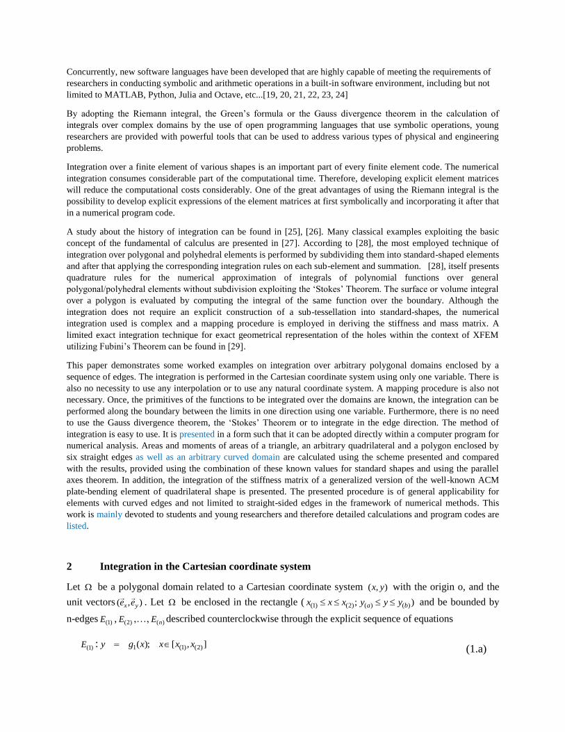
Figure 4: Polygonal domain enclosed by six straight edges, Cartesian coordinates of vertices, and edges
The exact values of the area of the polygonal cross section and the moments of area about the axes ),( yx
can be computed easily as difference between these values of a rectangle )1(A with the side length 68 and the
summation of them for four rectangled triangles )5()4()3()2( ,,, AAAA with the catheti 21 , 34 , 32 and 43 ,
Fig. 4 ( [32])
32)
2
)4)(3(
2
)3)(2(
2
)3)(4(
2
)2)(1(()6)(8(
)( )5()4()3()2()1(
AAAAAA
353.833333(4))3
22)(
2
)4)(3((
36
)4)(3(
(3))3
23(
2
)3)(2(
36
)3)(2(-(3))
3
1(
2
)3)(4(
36
)3)(4())
3
2(
2
)2)(1(
36
)2)(1({(-)
2
6)(6)(8(
12
)6)(8(
}{-
23
23
23
23
23
22222
22
)5()4()3()2()1(
AAAAA
AA
x
dAydAydAydAydAy
dxdyydAyI
x
y
)2( )3(
)6(
)4(
)2(A )3(A
)4(A
)4(E )5(A
)6(E
)1(A
)1(E
)2(E
)3(E
)5(E
)1(
)5(

580.833333(3))3
1)(
2
)3)(4((
36
)3)(4(
)3
46(
2
)3)(2(
36
)3)(2()
3
84)(
2
)3)(4((
36
)3)(4()
3
1(
2
)2)(1(
36
)1)(2({(-)
2
8)(8)(6(
12
)8)(6(
}{-
23
23
23
23
23
22222
22
)5()4()3()2()1(
AAAAA
AA
y
dAxdAxdAxdAxdAx
dxdyxdAxI
394.333333=Ix(4))3
2(3))(2
3
1)(
2
)4)(3((
72
)4)(3())3(
3
23((2))
3
26)(
2
)3)(2((
72
)3)(2(
))3(3
1((4))
3
24)(
2
)2)(4((
72
)3)(4())
3
2()
3
1((
2
)2)(1(
72
)2()1({(--)
2
6)(
2
8)(6)(8(0
}{-
2222
2222
)5()4()3()2()1(
AAAAA
AA
xy
xydAxydAxydAxydAxydA
xydxdyxydAI
The polygonal domain is bounded by six edges 654321 ,,,,, EEEEEE . Every edge-equation can be determined by the
two corresponding vertices spanning the edge. The resulting edge-equations solved with respect to y are as follows
Figure 5: Polygonal domain enclosed by six straight edges, subintervals of integration
1E : 22 xy
2E : 0y
3E : 34
3 xy
x
y
)1(
)3(
)6(
)4(
)2(A )3(A
)4(A
)5(E
)1(A
)1(E
)2(E
)3(E
)4(E
)6(E
)5(
)2(x )6(x )3(x )5(x )1(x )4(x
)5(A
)2(

4E : 152
3 xy
5E : 6y
6E : 23
4 xy
Moving in x -axes positive direction, the area of the polygon can be integrated after dividing the area A of the
polygon in five subareas )1(A , )2(A , )3(A , )4(A )5(A corresponding to the discontinuity points of the geometry as
follows, see Fig. 5
32)23
4()6()15
2
3()3
4
3()0()22(
|)(|)(|)(|)(|)(|)(
|)(|)(|)(|)(
|)(|)(|)(|)(|)(|)(
)()()()()(
0
3
3
6
6
8
8
4
4
1
1
0
0
3
6
3
6
5
6
8
4
8
4
3
4
1
2
1
0
1
8
6
3
8
6
4
6
4
3
6
4
5
4
3
2
4
3
5
3
1
2
3
1
6
1
0
1
1
0
6
8
6
6
4
4
3
3
1
1
0
5
3
5
2
5
2
6
2
6
1
)5()4()3()2()1(
dxxdxdxxdxxdxdxx
dxydxydxydxydxydxy
dxydxydxydxy
dxydxydxydxydxydxy
dxdydxdydxdydxdydxdy
dydxdydxdydxdydxdydxdydxA
EEEEEE
EEEE
EEEEEE
E
E
E
E
E
E
E
E
E
E
AAAAAA
In an analogous way, the moments of area about x -axes take the form
dxy
dxy
dxy
dxy
dxy
dxy
dxy
dxy
dxy
dxy
dxdyydxdyydxdyydxdyydxdyy
dydxydydxydydxydydxydydxydydxyI
EEEE
EEEEEE
E
E
E
E
E
E
E
E
E
E
AAAAAA
x
8
6
338
6
436
4
336
4
53
4
3
234
3
333
1
233
1
631
0
131
0
63
8
6
2
6
4
2
4
3
2
3
1
2
1
0
2
222222
3
|)(
3
|)(
3
|)(
3
|)(
3
|)(
3
|)(
3
|)(
3
|)(
3
|)(
3
|)(
)()()()()(
4
3
5
3
5
2
6
2
6
1
)5()4()3()2()1(
Rearranging the last integral counter clockwise gives:
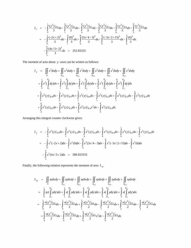
353.833333
)23/4(
3
)6(
3
)152/3(
3
)34/3(
3
)0(
3
)22(
3
|)(
3
|)(
3
|)(
3
|)(
3
|)(
3
|)(
0
3
3
3
6
36
8
38
4
34
1
31
0
3
0
3
533
6
436
8
338
4
234
1
131
0
63
dxx
dxdxx
dxx
dxdxx
dxy
dxy
dxy
dxy
dxy
dxy
I EEEEEEx
The moment of area about y -axes can be written as follows:
dxyxdxxyxdxyxdxyx
dxyxdxyxdxyxdxyxdxyxdxyx
dxdyxdxdyxdxdyxdxdyxdxdyx
dydxxdydxxdydxxdydxxdydxxdydxxI
EEEE
EEEEEE
E
E
E
E
E
E
E
E
E
E
AAAAAA
y
8
6
322
8
6
42
6
4
32
6
4
52
4
3
22
4
3
52
3
1
22
3
1
62
1
0
12
1
0
62
8
6
2
6
4
2
4
3
2
3
1
2
1
0
2
222222
|)(|)(|)(|)(
|)(|)(|)(|)(|)(|)(
)()()()()(
4
3
5
3
5
2
6
2
6
1
)5()4()3()2()1(
Arranging this integral counter clockwise gives:
580.833333)23/4(
)6()152/3()34/3()0()22(
|)(|)(|)(|)(|)(|)(
0
3
2
3
6
2
6
8
2
8
4
2
4
1
2
1
0
2
0
3
62
3
6
52
6
8
42
8
4
32
4
1
22
1
0
12
dxxx
dxxdxxxdxxxdxxdxxx
dxyxdxyxdxyxdxyxdxyxdxyxI EEEEEEy
Finally, the following relation represents the moment of area xyI
dxyx
dxxyx
dxyx
dxyx
dxyx
dxyx
dxyx
dxyx
dxyx
dxyx
dxydyxdxydyxdxydyxdxydyxdxydyxy
dyxydxdyxydxdyxydxdyxydxdyxydxdyxydxI
EEEE
EEEEEE
E
E
E
E
E
E
E
E
E
E
AAAAAA
xy
8
6
32
2
8
6
436
4
326
4
52
4
3
224
3
523
1
223
1
621
0
121
0
62
8
6
6
4
4
3
3
1
1
0
2
|)(
2
|)(
2
|)(
2
|)(
2
|)(
2
|)(
2
|)(
2
|)(
2
|)(
2
|)(
)()()()()(
4
3
5
3
5
3
6
2
6
1
)5()4()3()2()1(

This can be written in the following form:
394.3333332
)23/4(
2
)6(
2
)152/3(
2
)34/3(
2
)0(
2
)22(
2
|)(
2
|)(
2
|)(
2
|)(
2
|)(
2
|)(
0
3
2
3
6
26
8
28
4
24
1
21
0
2
0
3
623
6
526
8
428
4
324
1
221
0
12
dxxx
dxx
dxxx
dxxx
dxx
dxxx
dxyx
dxyx
dxyx
dxyx
dxyx
dxyx
I EEEEEExy
The same results can be obtained by dividing the polygon into two quadrilateral with the following nodal points
.2.0
.6.3
.6.6
.0.1
;
.6.6
.3.8
.0.4
.0.1
~
)(
~
)(ip
ip xx
and finding the explicit transformation relation between Cartesian variables and natural variables using the standard
bilinear approach and integrating the expressions for area and moments of area between -1 and +1.
In the following, a MATLAB function code is given by which the area and moments of area for an arbitrary polygon
with straight edges can be calculated.
Before using it, some notes on using formula (14) within a finite element program code must be considered. The
vertices of the polygonal domain must be ordered counterclockwise starting with the minimum x –value when
integrating over x or the smallest y –value when integrating over y in order to avoid any sign confusion which
leads to incorrect results. Furthermore, an edge equation of the form constx , when integrating over x or of the
form consty , when integrating over y must be avoided. In case of a parallel edge to x -axes the program will
stop running from itself (the code integrate over x ). The presented code is not intended for a general use in a finite
element program because it needs further editing to account for some special geometry cases of a polygon. It should
serve understanding and investigating the use of the Riemann formula in the current paper.
In order to call the code, the following script file must be saved under the name moa.m in the working directory.
%====================================moa.m=================================== % function for calculating moments of area of a Polygon with straight edges %============================================================================ function [A,Ix,Iy,Ixy]=moa(xip) n=size(xip); if (xip(1:1,1))< min(xip(2:n(1)-1,1)) syms x y; for i=1:n(1)-1 E(i)=det([ x y 1; xip(i,1) xip(i,2) 1; xip(i+1,1) xip(i+1,2) 1]); E(i)=solve(E(i),y); A(i)=-vpa(int(E(i),xip(i,1),xip(i+1,1))); Ix(i)=-vpa(int((E(i))^3/3,xip(i,1),xip(i+1,1))); Iy(i)=-vpa(int(x^2*E(i),xip(i,1),xip(i+1,1))); Ixy(i)=-vpa(int(x*(E(i))^2/2,xip(i,1),xip(i+1,1))); end
E(n(1))=det([ x y 1; xip(n(1),1) xip(n(1),2) 1; xip(1,1) xip(1,2) 1]);

E(n(1))=solve(E(n(1)),y); A(n(1))=-vpa(int(E(n(1)),xip(n(1),1),xip(1,1)));
Ix(n(1))=-vpa(int((E(n(1)))^3/3,xip(n(1),1),xip(1,1))); Iy(n(1))=-vpa(int(x^2*E(n(1)),xip(n(1),1),xip(1,1))); Ixy(n(1))=-vpa(int(x*(E(n(1)))^2/2,xip(n(1),1),xip(1,1)));
A=sum(transpose(A)); Ix=sum(transpose(Ix)); Iy=sum(transpose(Iy)); Ixy=sum(transpose(Ixy)); else fprintf('Please order the cordinate counter clockwise starting with the
smallest xip-one\n'); end
end %============================================================================
Calling the function for the triangle by the two following command lines
xip=[0 0 ; 5 0 ;1.8 2.4]
[A,Ix,Iy,Ixy]=moa(xip)
, for the quadrilateral by the two following command lines
xip=[1 1 ; 8 0 ;6 4 ; 2 5]
[A,Ix,Iy,Ixy]=moa(xip)
and finally for the polygon by the two following command lines
xip=[0 2;1 0;4 0;8 3;6 6;3 6]
[A,Ix,Iy,Ixy]=moa(xip)
give the results obtained in the three examples.
Example 4: Finally, a polygonal domain with five edges (Fig, 6) with the following Cartesian coordinates of
vertices
0.50.2
0.60.8
0.30.3
0.00.6
0.10.1
~
)(ipx
is computed using the above given program function and called by the two following command lines
xip=[1 1;6 0;3 3;8 6;2 5]
[A,Ix,Iy,Ixy]=moa(xip)
The output gives the following results for area and moments of area
A =15.5; Ix =186.08333333; Iy =218.75; Ixy =178.375

Figure 6: Polygonal domain enclosed by five straight edges, Cartesian coordinates of vertices, and edges
The same results can be obtained by dividing the polygon into two quadrilateral with the following nodal points
0.50.2
0.60.8
0.30.3
0.25.1
;
0.35.1
0.30.3
0.00.6
0.10.1
~
)(
~
)(ip
ip xx
and performing the integration using the standard bilinear approach.
Here, the results are also exact in case of non-convex polygon.
Example 5: The last assessment in this section is on a circular disc with a diameter of two units of length. The
circumference is divided into hundred segments. The above function moa(xip) is used along with the following
code:
% area and moments of area for a circular disc with a diameter of two units of length
i=0;
for f=-pi:pi/100:pi-pi/100
i=i+1
xip(i,1)=cos(f);xip(i,2)=sin(f);
end
xip
[A,Ix,Iy,Ixy]=moa(xip)
The output gives the following results
A =3.1410759078128293940787214943951;Ix =0.78513981600761063777789906861322
Iy =0.78513981600761063432172486883439; Ixy =-0.0000000000000000116128775033486671270401753.
x
y
)2(
)3(
)5( )4(
)4(E
)5(E
)1(E
)2(E
)3(E
)1(

(p) i~
These results are quasi correct (A=pi; Ix=Iy=pi/4 ; Ixy=0). It is worth mentioning that the convergence towards the
exact results occurs very slowly especially for the quadratic form of Ix or Iy. One can easily discover this fact by
changing the number of segments in the for loop.
Two reasons may delay the use of Riemann integral. Firstly, one needs to know the primitive of the function to be
integrated inside the domain. Secondly one needs also to express one variable using the other one explicitly at the
boundaries of the polygon, which is probably impossible in case of a complex geometry bounded by curves with
complex implicit expressions in the two variables. In the second case, one can use one-dimensional curve fitting
techniques to find explicit expressions at the domain boundaries.
7 Integration over domain with curved edges
Figure 7: Domain with curved edges, Cartesian coordinates of vertices, and edge-equations
Example 6: Let a four-sided curved domain defined by its four vertices (1), (2) (3), (4) (nodal points).
.5.1
.1.2
.0.1
.10
~
)(ipx
and enclosed by three curved edges and one straight edge. The edges are defined by the following edge-equations:
1:2 xyE
1)2(4: 23 xyE
21 1: xyE
14: 24 xyE
)1(
)4(
)3(
)2(
2A
5A 4A
3A 1A
x
y

]1,0[;)1(: 21 xxyE
]2,1[;1:2 xxyE
]2,1[;1)2(4: 23 xxyE
]1,0[;14: 24 xxyE
In order to calculate the exact values of the area and the moments of area of the curved domain using standard
elementary shapes, the five shapes shown in Fig. 7 are considered.
)1(A is the area of the unit quadrate with a unit side length.
)2(A is the area of a quarter bi-unit circle with a center located at the origin of the coordinate system .
)3(A is the area of the triangle with two edges of unit length.
)4(A , )5(A are the areas of the right and the left sub-parabolic segments with the side length 41 , respectively.
The area of the domain can now be calculated as follows
3.3812685)4)(1(
3
1)4)(1(
3
1)1)(1(
2
1)1)((
4
1)1)(1( 2
)5()4()3()2()1(
AAAAAA
Then, the moments of area read
15.548889))4(10
31)((4)(1(
3
1)4)(1(
2100
37
))4(10
31)((4)(1(
3
1)4)(1(
2100
37))1)(
3
2)((1)(1(
2
1)1)(1(
36
1)1)((
16
1)1)(1(
3
1
23
232343
)5()4()3()2()1(
xxxxxx IIIIII
3.9869838))4(4
11)((4)(1(
3
1)4()1(
80
1
))1(4
3)(4)(1(
3
1)4()1(
80
1))1)(
3
11)((1)(1(
2
1)1)(1(
36
1)1)((
16
1)1)(1(
3
1
23
232343
)5()4()3()2()1(
yyyyyy IIIIII
6.45))1(4
11))(4(
10
31)(4)(1(
3
1
))1)(1(4
3))(4)(1(
10
31)(4)(1(
3
1))1(
3
11)((1)(
3
2(
2
)1)(1()1()1(
72
1)21()1(
8
1)
2
1)(
2
1)(1)(1(
)
2222
)5()4()3()2()1(
xyxyxyxyxyxy IIIIII
Corresponding to the concept of the fundamental of calculus, the area of the curved domain can be calculated as
follows

(p) i~
3.3812685)14()1)2(4()1()1(
|)(|)(|)(|)(
|)(|)(|)(|)(
)()(
0
1
2
1
2
2
2
1
1
0
2
0
1
4
1
2
3
2
1
2
1
0
1
2
1
2
2
1
3
1
0
1
1
0
4
2
1
1
0
3
2
4
1
dxxdxxdxxdxx
dxydxydxydxy
dxydxydxydxy
dxdydxdydxdydAA
EEEE
EEEE
E
E
E
EAA
Then, the moments of area read
15.5488885
3
)14(
3
)1)2(4(
3
))1((
3
))1((
3
|)(
3
|)(
3
|)(
3
|)(
0
1
321
2
322
1
321
0
32
2
1
232
1
331
0
131
0
43
dxx
dxx
dxx
dxx
dxy
dxy
dxy
dxy
I EEEEx
3.9869838
)1)1(4()1)2(4()1())1((
|)(|)(|)(|)(
0
1
22
1
2
22
2
1
2
1
0
22
2
1
22
2
1
32
1
0
12
1
0
42
dxxxdxxxdxxxdxxx
dxyxdxyxdxyxdxyxI EEEEy
6.45
2
)14(
2
)1)2(4(
2
)1(
2
))1((
2
|)(
2
|)(
2
|)(
2
|)(
0
1
221
2
222
2
21
0
22
2
1
222
1
322
1
122
1
42
dxxx
dxxx
dxxx
dxxx
dxyx
dxyx
dxyx
dxyx
I EEEExy
Example 7: Let a four-sided curved domain defined by its four vertices (1), (2) (3), (4) (nodal points).
.5.2
.4.6
.0.8
.11
~
)(ipx
and enclosed by four curved parabolic segments . The edges are defined by the following edge-equations:

]8,1[;)8(49
1: 2
1 xxyE
]8,6[;)8(: 22 xxyE
]6,2[;4)6(16
1: 2
3 xxyE
]2,1[;1)1(4: 24 xxyE
Applying Eqn. (14) gives the following exact results
169.833333
387.733333
123.733333
20
x
y
x
I
I
I
a
The reader can easily verify these results by trying the following code
%============================================================================ % Area and Moments of area for a domain bounded by four parabolic segments %============================================================================ syms x y
%defining the quadrilateral curved domain
xip=[1 1;8 0;6 4;2 5] %vertices
%Edge equations
E(1)=(1/49)*((8-x)^2)
E(2)=(4/4)*((8.-x)^2)
E(3)=(1/16)*((6-x)^2)+4
E(4)=4*(1-x)^2+1
n=transpose(size(E))
for i=1:n(2)-1
A(i)=-vpa(int(E(i),xip(i,1),xip(i+1,1)))
Ix(i)=-vpa(int((E(i)^3/3),xip(i,1),xip(i+1,1)));
Iy(i)=-vpa(int(x^2*E(i),xip(i,1),xip(i+1,1)));
Ixy(i)=-vpa(int(x*(E(i)^2/2),xip(i,1),xip(i+1,1)));
end
A(n(2))=-vpa(int(E(n(2)),xip(n(2),1),xip(1,1)))
Ix(n(2))=-vpa(int((E(n(2))^3/3),xip(n(2),1),xip(1,1)));
Iy(n(2))=-vpa(int(x^2*E(n(2)),xip(n(2),1),xip(1,1)));
Ixy(n(2))=-vpa(int(x*(E(n(2))^2/2),xip(n(2),1),xip(1,1)));
A=sum(transpose(A)); A=vpa(A)
Ix=sum(transpose(Ix)); Ix=vpa(Ix)
Iy=sum(transpose(Iy)); Iy=vpa(Iy)

Ixy=sum(transpose(Ixy));Ixy=vpa(Ixy)
The last three examples show that the method is easily applicable for non-convex and complex domains.
7 Deriving the Stiffness matrix of a generalized ACM-plate bending element
The finite Element approximation is based on Hamilton’s Principle. The 2D expression for the special case of the
thin plate considered can be written in the absence of the prescribed boundary displacements relating to a Cartesian
coordinate system in the following form:
02
1
2
12
1
33
1
0
)(
)(0
dtuFdAuudAuqdAEt
t
n
iix
i
A A
j
ij
ixkl
A
ijkl
ij (17)
where
1t and 2t are two fixed time points of the vibration process, is the first variation,
A is the area and dA its differential element, iu is the velocity vector in which both displacement and rotation
components are included, ji is the corresponding mass density matrix, )(iF is the concentrated load applied at the
point (i).
ij is the curvature tensor, which reads expressed in terms of the deflection ),( 2103 xxu
x:
223
123
213
113
22
21
12
11
,
0
,
0
,
0
,
0
xxx
xxx
xxx
xxx
xx
xx
xx
xx
u
u
u
u
(18)
lkjiE is the matrix of the force-curvature dependency given in a matrix form as follows:
000
02/)1(2/)1(0
02/)1(2/)1(0
001
)1(12 2
3
EhEijkl
(19)
ji is defined by the following matrix:
12/00
012/0
00
3
3
h
hji
(20)
where is the material density, E is the modulus of elasticity, h is the plate thickness and the Poisson’s ratio
The indicial notation to indicate the Cartesian variables 21, xx is used instead of the yx, - frame and indices
between brackets range over the nodal points.
In Eqn. (17), the internal work associated with the bending and twist moments is only considered.

The plate finite element with the nodal points (i), (j), (k), (l) has three degrees of freedom each node. These are the
displacement normal to the plate surface in 3x -direction and the two rotations about
1x and 2x -axes. The total
number of degrees of freedom each element is then represented by the element nodal displacement vector with 12
degrees of freedom
)(nnu = {0
)(3 ixu ,
)(1 ix ,
)(2 ix ,
0
)(3 jxu ,
)(1 jx ,
)(2 jx ,
0
)(3 kxu ,
)(1 kx ,
)(2 kx ,
0
)(3 xu ,
)(1 x ,
)(2 x } (21)
The local axes 21, xx are defined using the directions of the element base vectors in an analogous procedure used in
section 4 in [33, 34]. The approximation basis is constructed using the defined local Cartesian variables 21, xx in the
usual parametric form [35, 36]:
)()(210 ),(3 mm
mm
xcMxxu
32123132221221312212121 )()()()()()()()(1 xxxxxxxxxxxyxxxxM
)4(3)2(1)1(1)( ..........cccc mm (22)
Linking the free parameters )(mmc to the nodal degrees of freedom using the essential boundary conditions at the
finite element level yield:
)()(
)()( mmmm
rrrr cAu (23)
Eliminating the free parameters from Eqn. (22) by solving the linear system of equations (23) and substituting the
result into equation (22), the following relationship between the internal displacements ),( 2103 xxu
x and the nodal
degrees of freedoms )(rru is obtained
)(1)(
)()(210 )),( (3 rr
mmrr
mm
xuAMxxu (24)
In Eqn. (23),)(
)(mm
rrA is a 1212 matrix derived from )(mmM by substituting the coordinates of the element nodes
and 1)(
)( )( mmrrA is the inverse matrix of
)()(mm
rrA .
Deriving the curvature tensor ij using Eqn. (24) yield
2121
222121
222121
2121
)(
)(1)(
)()(
60200200000
)(3)(30220010000
)(3)(30220010000
060026002000
)(
xxxx
xxxx
xxxx
xxxx
p
uAp
mm
rrmm
rrmm
ij
ij
ij
(25)
Applying the expressions of ij in the first term of Eqn. (17) gives
)()()(
)()(1)(
)()()(1)(
)()(2
1)))
2
1
2
1((( qq
qqrrrrqq
nnqq
nnijkl
A
mmmmrrrrkl
A
ijklij ukuuAdApEpAudAE
klij
(26)
where
1)()(
)()(1)()(
)()( ))) (((
nnqq
nnijkl
A
mmmmrr
qqrr AdApEpAkklij
(27)
is the element stiffness matrix related to the Cartesian coordinate system.
The integration over the area can be performed using the scheme presented above as follow:
n
i
E
x
x
nnmmnnijkl
x
mm
x
nnijkl
A
mm dxPdxdxpEpdApEpIi
i
i
rklijklij
1
1)()(12)()()()( |)()
)1(
)(1 2
( (28)
where )()( nnmm
rP is the primitive matrix of the 1212 matrix )()( nnijklmm
klijpEp with respect to
2x
2)()()()(
2
dxpEpP nnijkl
x
mmnnmm
klijr (29)
The stiffness matrix of the quadrilateral element of sec. 4 with the nodal coordinates
.5.2
.4.6
.0.8
.1.1
~
)(ipx
is derived. Defining a local coordinate system from the directions of the base vectors corresponding to [33], [34], the
new local coordinates read
2.43662.3185-
1.54801.7077
2.3950-3.8179
1.5896-3.2071-
)(ipx
The following two function code generate the stiffness matrix of the quadrilateral element
%============================Ekr.m==============================%
function [k]=EKr(xip,E,m,t)
%xip: local cartesian coordinates of the quadrilateral
%E: Young modulus m Poissons ratio t:thickness
%===============================================================%
syms x y ;
M=[ 1 x y x^2 x*y y^2 x^3 x^2*y x*y^2 y^3 x^3*y x*y^3];
Mxx=diff(diff(M,x),x);
Mxy=diff(diff(M,x),y);
Myy=diff(diff(M,y),y);
%c: eleasticity tensor in the x y-system
c=((E*t^3)/(12.*(1-m^2)))*[1 0 0 m; 0 (1-m)/2. (1-m)/2. 0; 0 (1-m)/2.
(1-m)/2. 0;m 0 0 1];
p=[Mxx;Mxy;Mxy;Myy];
Mi=[M;diff(M,y);-diff(M,x);];
A=[subs(subs(Mi,'x',xip(1,1)),'y',xip(1,2));
subs(subs(Mi,'x',xip(2,1)),'y',xip(2,2));subs(subs(Mi,'x',xip(3,1)),'y
',xip(3,2));subs(subs(Mi,'x',xip(4,1)),'y',xip(4,2))];
a=inv(A);
k=transpose(p)*c*p
%Primitive matrix of the matrix pT*c*p
k=int(k,y)
%integration over the boundary using x as variable

[kr]=Rk(k,xip)
k=transpose(a)*kr*a
eig(k)
%==============================EOF====================================
%==============================Rk.m===================================
% function for calculating stiffness matrix of a Polygon with straight
% edges using Riemann integral
% before call order the x-coordinate such that x(1)=min
%=====================================================================
function [kr]=Rk(k,xip)
n=size(xip);
if (xip(1:1,1))< min(xip(2:n(1)-1,1))
kr=zeros(12);
syms x y
for i=1:n(1)-1
E(i)=det([ x y 1; xip(i,1) xip(i,2) 1; xip(i+1,1) xip(i+1,2) 1]);
E(i)=solve(E(i),y);
kE=subs(k,y,E(i));
kr=kr-vpa(int(kE,xip(i,1),xip(i+1,1)));
end
E(i+1)=det([ x y 1; xip(n(1),1) xip(n(1),2) 1; xip(1,1) xip(1,2) 1]);
E(i+1)=solve(E(n(1)),y);
kE=subs(k,y,E(i));
Kr=kr-vpa(int(kE,xip(n(1),1),xip(1,1)));
vpa(kr,6);
else
fprintf('Please order the cordinate counter clockwise starting with
the smallest xip-one');
end
end
%===============================================================#
Calling the above two functions using the following three commands
xip =[ -3.2071 -1.5896; 3.8179 -2.3950; 1.7077 1.5480; -2.3185 2.4366]
EKr(xip,1365.0,0.3,0.2)
[kr]=Rk(k,xip)
produces the stiffness matrix and its eigenvalues listed in the first line of Tab. 1.
Table 1: Eigen values of the stiffness matrix of the quadrilateral element of sec. 4 related to a local Cartesian
coordinate system (integrated exactly using the Riemann integral)
1 2 3 4 5 6 7 8 9
26877.01 7835.507 58177253 2807...3 68.57.07 68032631 68013573 68717373 68201772
2286.126 78371301 58103713 28.67337 68.27230 68756320 68036..6 68751237 68203377

Similar results can be obtained by substituting the expressions for 21, xx derived using the standard bilinear
approach into Eqn. (27) between the limits -1, +1. The results of such procedure are listed cursive in the second line
of Tab.1.
Transforming the stiffness matrix into the global coordinate system gives the same results listed in Tab.1.
Performing the integration directly in the global coordinate system with the coordinates
xip=[1 1 ; 8 0 ;6 4 ; 2 5 ]
gives a very different results, which are lower by about 16%.
This example shows the necessity to define the proposed local element coordinate system and to locate it at the
geometric center of the element.
Similar procedure can be adopted to evaluate the element mass matrix resulting in from evaluating the third term of
Eqn. (17).
A final note about deriving the stiffness matrix of the rectangular ACM plate-bending element is to be mentioned. It
is better to use a separate program-code for deriving this matrix. The Fundamental of Calculus can deal with this
special case, too. For a rectangular element with the side-length ba ll and the origin of the coordinate system
located at the element center, the edges 2E and 4E lie on the coordinate lines alx ; alx , respectively. The
following simple code integrated using the Fundamental of Calculus in its ideal form gives the exact stiffness
matrix:
E(1)=-lb;E(3)=lb; kr=int(subs(k,y,E(3)),-la,la)-int(subs(k,y,E(1)),-la,la) where k is the primitive matrix of the matrix pT*c*p as constructed as in Ekr.m but now with the special nodal coordinates of the rectangular element. As may be seen, formula (14) or (15) applies in case of rectangular element, too, but only two edges have to be
considered during the integration.
Note that the results in the first seven examples using either formula (14) or the standard bilinear approach are exact
but the results of the stiffness matrix are different. In such cases, it is difficult to make right conclusions. A study on
benchmark of polygon quality metrics for polytopal element methods is still at the beginning [37]. However, one can
observe that the characters of the integrals in the first five examples are additive, whilst they are not additive when
deriving the stiffness matrix, which include the rotations and their derivatives. In addition the integrated shape
functions are discontinuous and non-conform. Therefore, we found ourselves confronted with similar problems that
appear during the discretization. Therefore, it is necessary to subject the element matrices to the same tests required
for a finite element application especially when the integrated function are discontinuous.
8 Changing the variable of integration
8.1. Using a polar coordinate system
An example of changing the variable of integration (i. e. x or y ) is the use of a polar coordinate
system. In polar coordinate system the following exact relations apply

sin
)/arccos(;;
cos
2222
ry
yxxyxr
rx
(30)
Note that x and y are replaced each by other two variables, namely ,r such that the Pythagorean Theorem applies.
In this sense, the transformation is exact and there is no approximation.
The position vector of an arbitrary point zyx ezeyexr
formulated in ,r terms reads
zyxzyx eererezeyexr
0sincos (31)
and the changes of it in ,r directions are as follows:
zyx
zyxr
eererdr
eeedrr
0cossin
0sincos
,
,
(32)
The deferential element of the area can now be calculated as a vector product of these changes
z
zyx
r erdrd
rr
eee
drdrrAd
0cossin
0sincos,, (34)
The integral over the area is now to be performed over the new variables
2
1
2
1
)(
)(
),(),(),(
rr
rrrA
ddrrrfddrrrfdxdyyxfI (35)
Usually, integration is first performed over the variable limits and after that over the constant limits.
8.2. Using a s, system
In the previous examples both limits of the integral change in x and y -direction even if the domain is bounded by
straight edges. Sometimes it is useful to use another coordinate system with one variant variable instead of using the
Cartesian coordinate system or a polar coordinate system. Therefore, it is more reliable to find other two variables
instead of x and y such that at least one of them has a constant value at the edges of the domain. Along the boundary
with straight edges both x and y change, but y has a constant value.
The idea now is to decompose the position vector r
into two vectors
and s
.
Let us define the position vector r
corresponding to the Chasles relation of vector addition as a sum of two vectors
s
,
rs
(36)

where,
is the position vector of an arbitrary point o of the plane 0z and s
the vector from o to p .
o can be located everywhere in the plane 0z .
An exact relation between the magnitude of s
, and of that of the position vector is then given by
22222 ),(cos2 ryxsss
(37)
where ss
, and rr
.
This relation is valid everywhere in the domain and along the boundaries with o as free selectable point.
In order to evaluate integrals such as A
dxdy or A
dxdyyxf ),( , yx, must be expressed in terms of s, .
In case of straight edges, after suitable selection of o , the relation between s, and yx, can be formulated at the
boundary. The integral can be performed in the s, instead of yx, .
The Wachspress space [38] offered an approximation basis for many publications dealing with polygonal and
polyhedral elements.
This idea can be extended by decomposing the position vector r
into more than two vectors
and s
when
necessary and useful. In any case the connection between the origin of the coordinate system yx, and o should not
be lost.
9 Conclusion
This paper shows the power of the Fundamental of Calculus in dealing with complex geometry-domains for some
practical engineering problems. The integration over a polygonal domain enclosed by a sequence of edges is
performed exactly using the Fundamental of Calculus without sub-division. Double integrals are transformed into
sequences of single integrals in one direction using the Fundamental of Calculus. There were no need to use the
Gauss divergence theorem, the ‘Stokes’ Theorem or to integrate in the edge direction. It was not necessary to use
any mapping procedure in order to integrate over a polygonal element. The presented way of integration is of
general applicability for convex and non-convex domains for a wide range of engineering and physical problems.
Some examples with curved edges are also investigated. The results are encouraging. Some notes on changing the
variables of the integration for instance, in case of using polar coordinate system or non-orthogonal coordinate
system are discussed.
10 References
[1] Weisstein, Eric W, M.ASCE, "Voronoi Diagram." From MathWorld--A Wolfram Web Resource.
http://mathworld.wolfram.com/VoronoiDiagram.html.
[2] Talischi C., Paulino G.H., Pereira A., Menezes I.F.M., Polymesher: a general-purpose mesh generator for
polygonal elements written in Matlab. Struct. Multidiscip. Optim., 45 (3) (2012), pp. 309-328.
[3] Gautam Dasgupta, M.ASCE, Integration within Polygonal Finite Elements, Journal of Aerospace
Engineering / January 2003/ 9, DOI: 10.1061/!ASCE"0893-1321!2003"16:1!9".

[4] Sukumar N, Tabarraei A, Conforming polygonal finite elements. Int J Numer Methods Eng. 2004;61:2045–
2066.
[5] Sommariva, A., Vianello, M., Product Gauss cubature over polygons based on Green's integration formula,
BIT Numerical Mathematics 47 (2007), 441—453.
[6] Manzini, G., Russo, A., Sukumar, N., New perspectives on polygonal and polyhedral finite element
methods, Mathematical Models and Methods in Applied Sciences, Vol. 24, No. 08, pp. 1665-1699 (2014).
[7] Chi, H., Talischi, C., Lopez-Pamies, O., Paulino, G.H., Polygonal finite elements for finite elasticity,
International Journal for Numerical Methods in Engineering, 101 (2015), pp. 305-328.
[8] Chi, H., Beirão da Veiga, L., Paulino, G.H. , Some basic formulations of the virtual element method (VEM)
for finite deformations. Computer Methods in Applied Mechanics and Engineering, Volume 318, 1 May
2017, pp. 148-192.
[9] Beirão da Veiga, L., Dassi, F., Russo, A., High-order Virtual Element Method on polyhedral meshes,
Computers & Mathematics with Applications, Volume 74, Issue 5, 1 September 2017, pp. 1110-1122.
[10] Wriggers, P., Rust, W.T., Reddy, B.D, A virtual element method for contact, Comput. Mech., 58 (6)
(2016), pp. 1039-1050.
[11] Chi, H., Talischi, C., Lopez-Pamies, O., Paulino, G. H., A paradigm for higher-order polygonal elements in
finite elasticity using a gradient correction scheme, Comput. Methods Appl. Mech. Engrg. 306 (2016) 216–
251, doi:10.1016/j.cma.2015.12.025.
[12] Beirão da Veiga, L., Russo, A., Vacca, G., The Virtual Element Method with curved edges, (2018),
arXiv:1711.04306v4[math.NA].
[13] Artioli, E., Sommariva, A., M. Vianello, M., Algebraic cubature on polygonal elements with a circular
edge, 2010 AMS subject classification: 65D32, 65N30, March 17, 2019 (in progress).
[14] Ho-Nguyen-Tan, T., Kim, H.-G., Polygonal shell elements with assumed transverse shear and membrane
strains, Computer Methods in Applied Mechanics and Engineering 349:(2019) 595-627.
[15] Wang, H, Qin QH, Lee, C, n-sided polygonal hybrid finite elements with unified fundamental solution
kernels for topology optimization, Applied Mathematical Modelling, vol. 66, no. (February 2019), pp. 97-
117.
[16] Shen, Z., Neil, T. R.,Robert, D., Drinkwater, B, W.,Holderied, M. W., Biomechanics of a moth scale at
ultrasonic frequencies, Proceedings of the National Academy of Sciences Nov 2018, 115 (48) 12200-
12205; DOI: 10.1073/pnas.1810025115.
[17] Kappert, K.D.R., van Alphen, M.J.A., van Dijk, S., Smeele,L.E., Balm, A.J.M., van der Heijden, F., An
interactive surgical simulation tool to assess the consequences of a partial glossectomy on a biomechanical
model of the tongue, Computer Methods in Biomechanics and Biomedical Engineering, 22:8, 827-839,
DOI: 10.1080/10255842.2019.1599362.
[18] Ferguson, J., Kópházi, J., Eaton, M. D., Polygonal Virtual Element Spatial Discretisation Methods for the
Neutron Diffusion Equation With Applications in Nuclear Reactor Physics, 2018 26th International
Conference on Nuclear Engineering, Volume 3: Nuclear Fuel and Material, Reactor Physics, and Transport
Theory, London, England, July 22–26, 2018., Paper No. ICONE26-81317, pp. V003T02A015; 7 pages,
doi:10.1115/ICONE26-81317.
[19] URL: https://julialang.org/

[20] URL: https://www.python.org/
[21] URL: https://www.mathworks.com/
[22] URL: http://www.wolfram.com/mathematica/
[23] URL: https://www.gnu.org/software/octave/
[24] Meurer A, Smith CP, Paprocki M, Čertík O, Kirpichev SB, Rocklin M, Kumar A, Ivanov S, Moore JK,
Singh S, Rathnayake T, Vig S, Granger BE, Muller RP, Bonazzi F, Gupta H, Vats S, Johansson F,
Pedregosa F, Curry MJ, Terrel AR, Roučka Š, Saboo A, Fernando I, Kulal S, Cimrman R, Scopatz A.
(2017) SymPy: symbolic computing in Python. PeerJ Computer Science 3:e103
https://doi.org/10.7717/peerj-cs.103.
[25] Hammarström, O., Origins of integration, Uppsala university, U.U.D.M. Project Report 2016:44, available
at URL:
https://pdfs.semanticscholar.org/eaa3/02ec2107d8668b2d12e8b9fc965217f33322.pdf
[26] Bastian, R., An introduction to the generalized Riemann integral and its role in undergraduate mathematics
education, Ashland University, December 2016. , available at URL:
https://etd.ohiolink.edu/!etd.send_file?accession=auhonors1482504144122774&disposition=inline
[27] Edelstein-Keshet, L., Integral Calculus with Applications to the Life Sciences, Mathematics Department,
University of British Columbia, Vancouver. Course notes for mathematics 103, February 26, 2014,
available at URL:
http://www.ugrad.math.ubc.ca/coursedoc/math103/2013W2/lecturenotes/lecturenotes.pdf
[28] Antonietti, P. F., Houston, P., Pennesi, G. , Fast Numerical integration on polytopic meshes with
applications to discontinuous Galerkin finite element methods, Journal of Scientific Computing, August
2018, DOI: 10.1007/s10915-018-0802-y. available at URL:
https://www.mate.polimi.it/biblioteca/add/qmox/03-2018.pdf.
[29] Perumal, L., Analysis of thin plates with holes by exact geometrical representation within XFEM, Journal
of Advanced Research. May 2016. Volume 7, Issue 3, pages 445 – 452, Volume 7, Issue 3, May 2016,
Pages 445-452.
http://dx.doi.org/10.1016/j.jare.2016.03.004
[30] Riemannintegral.EncyclopediaofMathematics.URL:
http://www.encyclopediaofmath.org/index.php?title=Riemann_integral&oldid=38637
[31] Wikipedia.URL: http://en.m.wiki.org/ Riemann_integral
[32] Timoshenko, S. and Young, D. H.: Engineering Mechanics, McGraw-Hill Book Company, Inc., New York,
(1940).
[33] Abo Diab, S.: Generalization of a reduced Trefftz-type approach, in B. Möller, Hrsg., Veröffent-lichungen
des Lehrstuhls für Statik., Technische Universität Dresden, Heft 4 (2001), Dresden (2001), p. 1-68.
[34] Abo Diab, S.: Quadrilateral folded plate structure elements of reduced Trefftz type, CAMES, vol. 10: No. 4,
(2003), p. 391-406.
[35] Melosh, R. J. A stiffness matrix for analysis of thin plates in bending, J. Aeronaut Sci, 1961, 28, pp. 34.
[36] Melosh, R. J. Basis for derivation of matrices for the direct stiffness analysis, AIAA J., 1, (1963), pp. 1631-
1637.

[37] Attene, M., Biasotti,S., Bertoluzza,S., Cabiddu, D., Livesu, M., Patané,G., Pennacchio, M., Prada, D.,
Spagnuolo, M., Benchmark of Polygon Quality Metrics for Polytopal Element Methods, Eurographics
Symposium on Geometry Processing 2019, D. Bommes and H. Huang, (Guest Editors), Volume 38 (2019),
Number 5.
[38] Wachspress, E. L., (1975). A Rational Finite Element Basis. Academic Press, New York, N.Y.
_________________________________________________________________________________________
Address: Sulaiman Abo Diab, Syria, Tartous, Hussain Al Baher
email: [email protected] or [email protected]
This research did not receive any specific grant from funding agencies in the public, commercial, or not-for-profit
sectors.


![La Integral Indefinida · La Integral Indefinida Definicion´ Sea f : [a;b] !R una funcion riemann integrable y acotada.´ Llamaremos INTEGRAL INDEFINIDA de f a la funcion´ F :](https://static.fdocuments.us/doc/165x107/5eba3c0536cf861e3c1ac9b7/la-integral-indefinida-la-integral-indeinida-deinicion-sea-f-ab-r-una.jpg)