WORD SENSE DISAMBIGUATION: SCALING UP, DOMAIN ADAPTATION …
153
WORD SENSE DISAMBIGUATION: SCALING UP, DOMAIN ADAPTATION, AND APPLICATION TO MACHINE TRANSLATION CHAN YEE SENG NATIONAL UNIVERSITY OF SINGAPORE 2008
Transcript of WORD SENSE DISAMBIGUATION: SCALING UP, DOMAIN ADAPTATION …

WORD SENSE DISAMBIGUATION:SCALING UP, DOMAIN ADAPTATION, ANDAPPLICATION TO MACHINE TRANSLATION
CHAN YEE SENG
NATIONAL UNIVERSITY OF SINGAPORE
2008
CORE Metadata, citation and similar papers at core.ac.uk
Provided by ScholarBank@NUS

WORD SENSE DISAMBIGUATION:SCALING UP, DOMAIN ADAPTATION, ANDAPPLICATION TO MACHINE TRANSLATION
CHAN YEE SENG(B.Computing (Hons.), NUS)
A THESIS SUBMITTEDFOR THE DEGREE OF DOCTOR OF PHILOSOPHY
DEPARTMENT OF COMPUTER SCIENCESCHOOL OF COMPUTING
NATIONAL UNIVERSITY OF SINGAPORE2008

Acknowledgments
The last four years have been one of the most exciting and defining period of my
life. Apart from experiencing the anxiousness while waiting for notifications of paper
submissions and the subsequent euphoria when they are accepted, I also met and
married my wife.
Doing research and working towards this thesis has been the main focus during
the past four years. I am grateful to my supervisor Dr. Hwee Tou Ng, whom I
have known since the year 2001, when I was starting on my honors year project as an
undergraduate student. His insights on the research field were instrumental in helping
me to focus on which research problems to tackle. He has also unreservedly shared
his vast research experience to mould me into a better and independent researcher.
I am also greatly thankful to my thesis committee, Dr. Wee Sun Lee and Dr. Chew
Lim Tan. Their valuable advice, be it on academic, research or life experiences, have
certainly been most enriching and helpful towards my work.
Many thanks also to Prof. Tat Seng Chua for his continued support all these
years. He and Dr. Hwee Tou Ng co-supervised my honors year project, which gave
me a taste of what doing research in Natural Language Processing is like. I would
also like to thank Dr. Min-Yen Kan for his help and advice which are unreservedly
given whenever I approached him. Thanks also to Dr. David Chiang, for his valuable
i

insights and induction into the field of Machine Translation.
Thanks also to my friends and colleagues from the Computational Linguistics lab:
Shan Heng Zhao, Muhua Zhu, Upali Kohomban, Hendra Setiawan, Zhi Zhong, Wei
Lu, Hui Zhang, Thanh Phong Pham, and Zheng Ping Jiang. Many thanks for their
support during the daily grind of working towards a research paper, for the many
insightful discussions, and also for the wonderful and fun outings that we had.
One of the most important people who has been with me throughout my PhD
studies is my wife Yu Zhou. It was with her love, unwavering support, and unques-
tioning belief in whatever I’m doing that gave me the strength and confidence to
persevere during the many frustrating moments of my research. Plus, she also put
up with the many nights when I had to work late in our bedroom.
Finally, many thanks to my parents, family, and friends, for their support and
understanding. Thanks also to Singapore Millennium Foundation and National Uni-
versity of Singapore for funding my PhD studies.
ii

Contents
Acknowledgments i
Summary vii
1 Introduction 1
1.1 Word Sense Disambiguation . . . . . . . . . . . . . . . . . . . . . . . 1
1.2 SENSEVAL . . . . . . . . . . . . . . . . . . . . . . . . . . . . . . . . 2
1.3 Research Problems in Word Sense Disambiguation . . . . . . . . . . . 5
1.3.1 The Data Acquisition Bottleneck . . . . . . . . . . . . . . . . 6
1.3.2 Different Sense Priors Across Domains . . . . . . . . . . . . . 7
1.3.3 Perceived Lack of Applications for Word Sense Disambiguation 9
1.4 Contributions of this Thesis . . . . . . . . . . . . . . . . . . . . . . . 11
1.4.1 Tackling the Data Acquisition Bottleneck . . . . . . . . . . . . 11
1.4.2 Domain Adaptation for Word Sense Disambiguation . . . . . . 12
1.4.3 Word Sense Disambiguation for Machine Translation . . . . . 14
1.4.4 Research Publications . . . . . . . . . . . . . . . . . . . . . . 14
1.5 Outline of this Thesis . . . . . . . . . . . . . . . . . . . . . . . . . . . 16
2 Related Work 18
iii

2.1 Acquiring Training Data for Word Sense Disambiguation . . . . . . . 19
2.2 Domain Adaptation for Word Sense Disambiguation . . . . . . . . . . 23
2.3 Word Sense Disambiguation for Machine Translation . . . . . . . . . 24
3 Our Word Sense Disambiguation System 27
3.1 Knowledge Sources . . . . . . . . . . . . . . . . . . . . . . . . . . . . 27
3.1.1 Local Collocations . . . . . . . . . . . . . . . . . . . . . . . . 28
3.1.2 Part-of-Speech (POS) of Neighboring Words . . . . . . . . . . 28
3.1.3 Surrounding Words . . . . . . . . . . . . . . . . . . . . . . . . 28
3.2 Learning Algorithms and Feature Selection . . . . . . . . . . . . . . . 29
3.2.1 Performing English Word Sense Disambiguation . . . . . . . . 29
3.2.2 Performing Chinese Word Sense Disambiguation . . . . . . . . 30
4 Tackling the Data Acquisition Bottleneck 32
4.1 Gathering Training Data from Parallel Texts . . . . . . . . . . . . . . 33
4.1.1 The Parallel Corpora . . . . . . . . . . . . . . . . . . . . . . . 33
4.1.2 Selection of Target Translations . . . . . . . . . . . . . . . . . 35
4.2 Evaluation on English All-words Task . . . . . . . . . . . . . . . . . . 38
4.2.1 Selection of Words Based on Brown Corpus . . . . . . . . . . 38
4.2.2 Manually Sense-Annotated Corpora . . . . . . . . . . . . . . . 40
4.2.3 Evaluations on SENSEVAL-2 and SENSEVAL-3 English all-
words Task . . . . . . . . . . . . . . . . . . . . . . . . . . . . 40
4.3 Evaluation on SemEval-2007 . . . . . . . . . . . . . . . . . . . . . . . 46
4.3.1 Sense Inventory . . . . . . . . . . . . . . . . . . . . . . . . . . 47
4.3.2 Fine-Grained English All-words Task . . . . . . . . . . . . . . 48
4.3.3 Coarse-Grained English All-words Task . . . . . . . . . . . . . 49
iv
4.4 Sense-tag Accuracy of Parallel Text Examples . . . . . . . . . . . . . 52
4.5 Summary . . . . . . . . . . . . . . . . . . . . . . . . . . . . . . . . . 55
5 Word Sense Disambiguation with Sense Prior Estimation 56
5.1 Estimation of Priors . . . . . . . . . . . . . . . . . . . . . . . . . . . 57
5.1.1 Confusion Matrix . . . . . . . . . . . . . . . . . . . . . . . . . 57
5.1.2 EM-Based Algorithm . . . . . . . . . . . . . . . . . . . . . . . 60
5.1.3 Predominant Sense . . . . . . . . . . . . . . . . . . . . . . . . 62
5.2 Using A Priori Estimates . . . . . . . . . . . . . . . . . . . . . . . . . 63
5.3 Calibration of Probabilities . . . . . . . . . . . . . . . . . . . . . . . . 64
5.3.1 Well Calibrated Probabilities . . . . . . . . . . . . . . . . . . 64
5.3.2 Being Well Calibrated Helps Estimation . . . . . . . . . . . . 65
5.3.3 Isotonic Regression . . . . . . . . . . . . . . . . . . . . . . . . 66
5.4 Selection of Dataset . . . . . . . . . . . . . . . . . . . . . . . . . . . . 69
5.4.1 DSO Corpus . . . . . . . . . . . . . . . . . . . . . . . . . . . 70
5.4.2 Parallel Texts . . . . . . . . . . . . . . . . . . . . . . . . . . . 70
5.5 Results Over All Words . . . . . . . . . . . . . . . . . . . . . . . . . . 71
5.5.1 Experimental Results . . . . . . . . . . . . . . . . . . . . . . . 73
5.6 Sense Priors Estimation with Logistic Regression . . . . . . . . . . . 77
5.7 Experiments Using True Predominant Sense Information . . . . . . . 80
5.8 Experiments Using Predicted Predominant Sense Information . . . . 83
5.9 Summary . . . . . . . . . . . . . . . . . . . . . . . . . . . . . . . . . 85
6 Domain Adaptation with Active Learning for Word Sense Disam-
biguation 87
6.1 Experimental Setting . . . . . . . . . . . . . . . . . . . . . . . . . . . 88
v

6.1.1 Choice of Corpus . . . . . . . . . . . . . . . . . . . . . . . . . 89
6.1.2 Choice of Nouns . . . . . . . . . . . . . . . . . . . . . . . . . . 89
6.2 Active Learning . . . . . . . . . . . . . . . . . . . . . . . . . . . . . . 90
6.3 Count-merging . . . . . . . . . . . . . . . . . . . . . . . . . . . . . . 92
6.4 Experimental Results . . . . . . . . . . . . . . . . . . . . . . . . . . . 93
6.4.1 Utility of Active Learning and Count-merging . . . . . . . . . 94
6.4.2 Using Sense Priors Information . . . . . . . . . . . . . . . . . 94
6.4.3 Using Predominant Sense Information . . . . . . . . . . . . . 95
6.5 Summary . . . . . . . . . . . . . . . . . . . . . . . . . . . . . . . . . 100
7 Word Sense Disambiguation for Machine Translation 101
7.1 Hiero . . . . . . . . . . . . . . . . . . . . . . . . . . . . . . . . . . . . 102
7.1.1 New Features in Hiero for WSD . . . . . . . . . . . . . . . . . 104
7.2 Gathering Training Examples for WSD . . . . . . . . . . . . . . . . . 106
7.3 Incorporating WSD during Decoding . . . . . . . . . . . . . . . . . . 107
7.4 Experiments . . . . . . . . . . . . . . . . . . . . . . . . . . . . . . . . 111
7.4.1 Hiero Results . . . . . . . . . . . . . . . . . . . . . . . . . . . 112
7.4.2 Hiero+WSD Results . . . . . . . . . . . . . . . . . . . . . . . 113
7.5 Analysis . . . . . . . . . . . . . . . . . . . . . . . . . . . . . . . . . . 113
7.6 Summary . . . . . . . . . . . . . . . . . . . . . . . . . . . . . . . . . 117
8 Conclusion 118
8.1 Future Work . . . . . . . . . . . . . . . . . . . . . . . . . . . . . . . . 119
8.1.1 Acquiring Examples from Parallel Texts for All English Words 120
8.1.2 Word Sense Disambiguation for Machine Translation . . . . . 120
vi

Summary
The process of identifying the correct meaning, or sense of a word in context, is known
as word sense disambiguation (WSD). This thesis explores three important research
issues for WSD.
Current WSD systems suffer from a lack of training examples. In our work, we
describe an approach of gathering training examples for WSD from parallel texts. We
show that incorporating parallel text examples improves performance over just using
manually annotated examples. Using parallel text examples as part of our training
data, we developed systems for the SemEval-2007 coarse-grained and fine-grained
English all-words tasks, obtaining excellent results for both tasks.
In training and applying WSD systems on different domains, an issue that affects
accuracy is that instances of a word drawn from different domains have different sense
priors (the proportions of the different senses of a word). To address this issue, we
estimate the sense priors of words drawn from a new domain using an algorithm based
on expectation maximization (EM). We show that the estimated sense priors help to
improve WSD accuracy. We also use this EM-based algorithm to detect a change in
predominant sense between domains. Together with the use of count-merging and
active learning, we are able to perform effective domain adaptation to port a WSD
system to new domains.
vii

Finally, recent research presents conflicting evidence on whether WSD systems
can help to improve the performance of statistical machine translation (MT) systems.
In our work, we show for the first time that integrating a WSD system achieves a
statistically significant improvement on the translation performance of Hiero, a state-
of-the-art statistical MT system.
viii

List of Tables
4.1 Size of English-Chinese parallel corpora . . . . . . . . . . . . . . . . . 34
4.2 WordNet sense descriptions and assigned Chinese translations of the
noun channel . . . . . . . . . . . . . . . . . . . . . . . . . . . . . . . 36
4.3 POS tag and lemma prediction accuracies for SENSEVAL-2 (SE-2)
and SENSEVAL-3 (SE-3) English all-words task. . . . . . . . . . . . 41
4.4 SENSEVAL-2 English all-words task evaluation results. . . . . . . . . 41
4.5 SENSEVAL-3 English all-words task evaluation results. . . . . . . . . 41
4.6 Paired t-test between the various results over all the test examples of
SENSEVAL-2 English all-words task. “∼”, (“>” and “<”), and (“À”
and “¿”) correspond to the p-value > 0.05, (0.01, 0.05], and ≤ 0.01
respectively. For instance, the ¿ between WNS1 and PT means that
PT is significantly better than WNS1 at a p-value of ≤ 0.01. . . . . 45
4.7 Paired t-test between the various results over all the test examples of
SENSEVAL-3 English all-words task. . . . . . . . . . . . . . . . . . . 45
ix

4.8 Scores for the SemEval-2007 fine-grained English all-words task, using
different sets of training data. SC+DSO refers to using examples gath-
ered from SemCor and DSO corpus. Similarly, SC+DSO+PT refers
to using examples gathered from SemCor, DSO corpus, and paral-
lel texts. SC+DSO+PTnoun is similar to SC+DSO+PT, except that
parallel text examples are only gathered for nouns. Similarly, PTverb
means that parallel text examples are only gathered for verbs. . . . . 48
4.9 Scores for the SemEval-2007 coarse-grained English all-words task, us-
ing different sets of training data. . . . . . . . . . . . . . . . . . . . . 49
4.10 Score of each individual test document, for the SemEval-2007 coarse-
grained English all-words task. . . . . . . . . . . . . . . . . . . . . . . 49
4.11 Sense-tag analysis over 1000 examples . . . . . . . . . . . . . . . . . . 52
5.1 Number of words with different or the same predominant sense (PS)
between the training and test data. . . . . . . . . . . . . . . . . . . . 71
5.2 Micro-averaged WSD accuracies over all the words, using the various
methods. The naive Bayes here are multiclass naive Bayes (NB). . . . 72
5.3 Relative accuracy improvement based on non-calibrated probabilities. 72
5.4 Micro-averaged WSD accuracies over all the words, using the various
methods. The naive Bayes classifiers here are with calibrated proba-
bilities (NBcal). . . . . . . . . . . . . . . . . . . . . . . . . . . . . . . 76
5.5 Relative accuracy improvement based on calibrated probabilities. . . 76
5.6 Micro-averaged WSD accuracies using the various methods, for the set
of words having different predominant senses between the training and
test data. The different naive Bayes classifiers are: multiclass naive
Bayes (NB) and naive Bayes with calibrated probabilities (NBcal). . . 81
x

5.7 Relative accuracy improvement based on uncalibrated probabilities. . 81
5.8 Relative accuracy improvement based on calibrated probabilities. . . 81
5.9 Paired t-tests between the various methods for the four datasets. Here,
logistic regression is abbreviated as logR and calibration as cal. . . . 81
5.10 Number of words with different or the same predominant sense (PS)
between the training and test data. Numbers in brackets give the
number of words where the EM-based algorithm predicts a change in
predominant sense. . . . . . . . . . . . . . . . . . . . . . . . . . . . . 84
5.11 Micro-averaged WSD accuracies over the words with predicted different
predominant senses between the training and test data. . . . . . . . . 84
5.12 Relative accuracy improvement based on uncalibrated probabilities. . 84
5.13 Relative accuracy improvement based on calibrated probabilities. . . 84
6.1 The average number of senses in BC and WSJ, average MFS accuracy,
average number of BC training, and WSJ adaptation examples per noun. 90
6.2 Annotation savings and percentage of adaptation examples needed to
reach various accuracies. . . . . . . . . . . . . . . . . . . . . . . . . . 99
7.1 BLEU scores . . . . . . . . . . . . . . . . . . . . . . . . . . . . . . . 112
7.2 Weights for each feature obtained by MERT training. The first eight
features are those used by Hiero in Chiang (2005). . . . . . . . . . . . 112
7.3 Number of WSD translations used and proportion that matches against
respective reference sentences. WSD translations longer than 4 words
are very sparse (less than 10 occurrences) and thus they are not shown. 114
xi

List of Figures
1.1 Performance of systems in the SENSEVAL-2 English all-words task.
The single shaded bar represents the baseline strategy of using first
WordNet sense, the empty white bars represent the supervised systems,
and the pattern-filled bars represent the unsupervised systems. . . . 3
1.2 Performance of systems in the SENSEVAL-3 English all-words task. . 3
4.1 An occurrence of channel aligned to a selected Chinese translation. . 36
5.1 Sense priors estimation using the confusion matrix algorithm. . . . . 58
5.2 Sense priors estimation using the EM algorithm. . . . . . . . . . . . . 63
5.3 PAV algorithm. . . . . . . . . . . . . . . . . . . . . . . . . . . . . . . 67
5.4 PAV illustration. . . . . . . . . . . . . . . . . . . . . . . . . . . . . . 67
5.5 Sense priors estimation using the EM algorithm with calibration. . . . 75
5.6 Sense priors estimation with logistic regression. . . . . . . . . . . . . 78
6.1 Active learning . . . . . . . . . . . . . . . . . . . . . . . . . . . . . . 91
6.2 Adaptation process for all 21 nouns. In the graph, the curves are: r
(random selection), a (active learning), a-c (active learning with count-
merging), a-truePrior (active learning, with BC examples gathered to
adhere to true sense priors in WSJ). . . . . . . . . . . . . . . . . . . 93
xii

6.3 Using true predominant sense for the 9 nouns. The curves are: a (active
learning), a-truePrior (active learning, with BC examples gathered to
adhere to true sense priors in WSJ), a-truePred (active learning, with
BC examples gathered such that its predominant sense is the same as
the true predominant sense in WSJ). . . . . . . . . . . . . . . . . . . 97
6.4 Using estimated predominant sense for the 9 nouns. The curves are:
r (random selection), a (active learning), a-truePred (active learning,
with BC examples gathered such that its predominant sense is the
same as the true predominant sense in WSJ), a-estPred (similar to a-
truePred, except that the predominant sense in WSJ is estimated by
the EM-based algorithm), a-c-estPred (employing count-merging with
a-estPred). . . . . . . . . . . . . . . . . . . . . . . . . . . . . . . . . 98
7.1 An example derivation which consists of 8 grammar rules. The source
string of each rule is represented by the box before the comma, while
the shaded boxes represent the target strings of the rules. . . . . . . . 103
7.2 We perform WSD on the source string “c5”, using the derived context
dependent probability to change the original cost of the grammar rule. 105
7.3 WSD translations affecting the cost of a rule R considered during de-
coding. . . . . . . . . . . . . . . . . . . . . . . . . . . . . . . . . . . . 108
xiii

Chapter 1
Introduction
1.1 Word Sense Disambiguation
Many words have multiple meanings. For example, in the sentence “The institu-
tions have already consulted the staff concerned through various channels, including
discussion with the staff representatives”, the word channel denotes a means of com-
munication or access. However, in the sentence “A channel is typically what you rent
from a telephone company”, the word channel refers to a path over which electrical
signals can pass. The process of identifying the correct meaning, or sense of a word
in context, is known as word sense disambiguation (WSD) (Ng and Zelle, 1997). This
is one of the fundamental problems in natural language processing (NLP).
In the typical setting, WSD is a classification problem where each ambiguous
word is assigned a sense label, usually from a pre-defined sense inventory, during
the disambiguation process. Being able to accurately disambiguate word sense is
important for applications such as information retrieval, machine translation, etc.
In current WSD research, WordNet (Miller, 1990) is usually used as the sense
1

CHAPTER 1. INTRODUCTION 2
inventory. WordNet is a semantic lexicon for the English language, where words
are organized into synonym sets (called synsets), with various semantic relations
between these synonym sets. As an example, nouns are organized as a hierarchical
structure based on hypernymy and hyponymy1 relations. Thus, unlike a standard
dictionary which merely lists word definitions in an alphabetical order, the conceptual
organization of WordNet makes it a useful resource for NLP research.
1.2 SENSEVAL
Driven by a lack of standardized datasets and evaluation metics, a series of evalua-
tion exercises called SENSEVAL were held. These exercises evaluated the strengths
and weaknesses of WSD algorithms and participating systems created by research
communities worldwide, with respect to different words and different languages.
SENSEVAL-1 (Kilgarriff, 1998), the first international workshop on evaluating
WSD systems, was held in the summer of 1998, under the auspices of ACL SIGLEX
(the Special Interest Group on the Lexicon of the Association for Computational
Linguistics) and EURALEX (European Association for Lexicography). SENSEVAL-
1 uses the HECTOR (Atkins, 1992) sense inventory.
SENSEVAL-2 (Edmonds and Cotton, 2001) took place in the summer of 2001.
Two of the tasks in SENSEVAL-2 were the English all-words task (Palmer et al.,
2001), and the English lexical sample task (Kilgarriff, 2001). In SENSEVAL-2,
WordNet-1.7 was used as the sense inventory for these two tasks. A brief description
of these two tasks follows.
• English all-words task: Systems must tag almost all of the content words (words
1Y is a hypernym of X if X is a (kind of) Y. X is a hyponym of Y if X is a (kind of) Y

CHAPTER 1. INTRODUCTION 3
0
10
20
30
40
50
60
70
80
90
100
WS
D F
1-sc
ore
SE2 System Performance
69.0
63.6
62.0
61.8
47.3
46.4
46.3
38.6
57.2
55.3
48.3
45.1
43.3
36.0
34.1
33.6
27.5
26.0
25.8
22.7
6.8
6.1
5.9
SupervisedWNS1
Unsupervised
Figure 1.1: Performance of systems in the SENSEVAL-2 Englishall-words task. The single shaded bar represents the baseline strat-egy of using first WordNet sense, the empty white bars representthe supervised systems, and the pattern-filled bars represent theunsupervised systems.
0
10
20
30
40
50
60
70
80
90
100
WS
D F
1-sc
ore
SE3 System Performance
65.1
64.6
64.3
62.6
62.4
61.9
61.0
61.0
61.0
59.4
57.6
56.2
56.0 58
.2
56.7
55.1
55.0
52.6
51.8
50.3
46.5
46.1
46.0
45.3
43.5
40.6
30.5
SupervisedWNS1
Unsupervised
Figure 1.2: Performance of systems in the SENSEVAL-3 Englishall-words task.

CHAPTER 1. INTRODUCTION 4
having the part-of-speech noun, adjective, verb, or adverb) in a sample of run-
ning English text. No training data is provided for this task.
• English lexical sample task: Systems must tag instances of a selected sample of
English words, where the instances are presented as short extracts of English
text. A relatively large amount of annotated data, where the predetermined
words are tagged in context, are provided as training data for this task.
Following the success of SENSEVAL-2, SENSEVAL-3 was held in the summer of
2004. Similar to SENSEVAL-2, two of the tasks for the English language are the
English all-words task (Snyder and Palmer, 2004) and the English lexical sample task
(Mihalcea, Chklovski, and Kilgarriff, 2004). The WordNet-1.7.1 sense inventory was
used for these two tasks.
The SENSEVAL-2 and SENSEVAL-3 exercises show that among the various ap-
proaches to WSD, corpus-based supervised machine learning methods are the most
successful. With this approach, one needs to obtain a corpus where each occurrence
of an ambiguous word had been earlier manually annotated with the correct sense,
according to some existing sense inventory, to serve as training data.
In WordNet, the senses of each word are ordered in terms of their frequency of
occurrence in the English texts in the SemCor corpus (Miller et al., 1994), which
is part of the Brown Corpus (BC) (Kucera and Francis, 1967). Since these texts are
general in nature and do not belong to any specific domain, the first WordNet sense
of each word is generally regarded as its most common sense. Hence, to gauge the
performance of state-of-the-art supervised WSD systems, we investigate the perfor-
mance of a baseline strategy which simply tags each word with its first WordNet sense.
On the English all-words task of SENSEVAL-2, this strategy achieves an accuracy of
62.0%. As shown in Figure 1.1, only two participating systems achieve performance

CHAPTER 1. INTRODUCTION 5
better than this baseline accuracy. When applied on the English all-words task of
SENSEVAL-3, the baseline strategy achieves an accuracy of 61.9%. As shown in Fig-
ure 1.2, only a few participating systems perform better than this baseline strategy
and their accuracy improvements are marginal.
1.3 Research Problems in Word Sense Disambigua-
tion
Results of SENSEVAL-2 and SENSEVAL-3 English all-words task show that super-
vised systems are more successful than unsupervised systems. The results also show,
however, that current state-of-the-art supervised WSD systems still find it hard to
outperform a simple WordNet first sense strategy on a consistent basis.
One problem the supervised systems currently face is a lack of a large amount
of sense-tagged data for training. The sense annotation process is usually done by
trained lexicographers and the obvious drawback here is the laborious manual sense-
tagging involved. This problem is particularly severe for WSD, since sense-tagged
data have to be collected for each ambiguous word of a language. Due to the laborious
and expensive annotation process, as of today, only a handful of sense-tagged corpora
are publicly available.
Another equally pressing problem that arises out of supervised learning is the
issue of domain dependence. A WSD system trained on data from one domain, e.g.,
sports, will show a decrease in performance when applied on a different domain, e.g.,
economics. Tackling this problem is necessary for building scalable and wide-coverage
WSD systems that are portable across different domains.
The third problem is the perceived lack of applications for WSD. Traditionally,

CHAPTER 1. INTRODUCTION 6
WSD is evaluated as an isolated task, without regard to any specific application.
Hence, doubts have been expressed on the utility of WSD for actual NLP applications.
1.3.1 The Data Acquisition Bottleneck
Among the existing sense-tagged corpora, the SemCor corpus (Miller et al., 1994)
is one of the most widely used. In SemCor, content words have been manually
tagged with word senses from the WordNet sense inventory. Current supervised WSD
systems (such as participants in the SENSEVAL English all-words task) usually rely
on this relatively small manually annotated corpus for training examples. However,
this has affected the scalability and performance of these systems. As we have shown
in Figures 1.1 and 1.2, very few SENSEVAL participating systems perform better
than the baseline WordNet first sense strategy.
In order to build wide-coverage and scalable WSD systems, tackling the data ac-
quisition bottleneck for WSD is crucial. In an attempt to do this, the DSO corpus
(Ng and Lee, 1996; Ng, 1997a) was manually annotated. It consists of 192,800 word
occurrences of 121 nouns and 70 verbs. In another attempt to collect large amounts
of sense-tagged data, Chklovski and Mihalcea initiated the Open Mind Word Ex-
pert (OMWE) project (Chklovski and Mihalcea, 2002) to collect sense-tagged data
from Internet users. Data gathered through the OMWE project were used in the
SENSEVAL-3 English lexical sample task. In that task, WordNet-1.7.1 was used as
the sense inventory for nouns and adjectives, while Wordsmyth2 was used as the sense
inventory for verbs.
Although the DSO corpus and OMWE project are good initiatives, sense annota-
tion is still done manually and this inherently limits the amount of data that can be
2http://www.wordsmyth.net

CHAPTER 1. INTRODUCTION 7
collected. As proposed by Resnik and Yarowsky, a source of potential training data is
parallel texts (Resnik and Yarowsky, 1997), where translation distinctions in a target
language can potentially serve as sense distinctions in the source language. In a later
work (Resnik and Yarowsky, 2000), the authors investigated the probability that 12
different languages will differently lexicalize the senses of English words. They found
that there appears to be a strong association with language distance from English, as
non-Indo-European languages in general have a higher probability to differently lexi-
calize English senses, as compared to Indo-European languages. From their study, the
Basque language has the highest probability of differently lexicalizing English senses,
followed by Japanese, Korean, Chinese, Turkish, and so on.
To explore the potential of this approach, our prior work (Ng, Wang, and Chan,
2003) exploited English-Chinese parallel texts for WSD. For each noun of SENSEVAL-
2 English lexical sample task, we provided some Chinese translations for each of the
senses. Senses were lumped together if they were translated in the same way in
Chinese. Given a word-aligned English-Chinese parallel corpus, these different Chi-
nese translations then serve as the “sense-tags” of the corresponding English noun.
Through this approach, we gathered training examples for WSD from parallel texts.
Note that the examples are collected without manually annotating each individual
ambiguous word occurrence, thus allowing us to gather the examples in a much shorter
time. In (Ng, Wang, and Chan, 2003), we obtained encouraging results in our evalu-
ation on the nouns of SENSEVAL-2 English lexical sample task.
1.3.2 Different Sense Priors Across Domains
The reliance of supervised WSD systems on annotated corpus raises the important
issue of domain dependence. To investigate this, Escudero, Marquez, and Rigau

CHAPTER 1. INTRODUCTION 8
(2000) and Martinez and Agirre (2000) conducted experiments using the DSO corpus,
which contains sentences from two different corpora, namely Brown Corpus (BC)
and Wall Street Journal (WSJ). They found that training a WSD system on one
part (BC or WSJ) of the DSO corpus, and applying it to the other can result in an
accuracy drop of more than 10%. A reason given by the authors is that examples
from different domains will exhibit greater differences such as variation in collocations,
thus presenting different classification cues to the learning algorithm. Another reason
pointed out in (Escudero, Marquez, and Rigau, 2000) is the difference in sense priors
(i.e., the proportions of the different senses of a word) between BC and WSJ. For
instance, the noun interest has these 6 senses in the DSO corpus: sense 1, 2, 3, 4, 5,
and 8. In the BC part of the DSO corpus, these senses occur with the proportions:
34%, 9%, 16%, 14%, 12%, and 15%. However, in the WSJ part of the DSO corpus,
the proportions are different: 13%, 4%, 3%, 56%, 22%, and 2%. When the authors
assumed they knew the sense priors of each word in BC and WSJ, and adjusted these
two datasets such that the proportions of the different senses of each word were the
same between BC and WSJ, accuracy improved by 9%. In another work, Agirre and
Martinez (2004) trained a WSD system on data which was automatically gathered
from the Internet. The authors reported a 14% improvement in accuracy if they
have an accurate estimate of the sense priors in the evaluation data and sampled
their training data according to these sense priors. The work of these researchers
showed that when the domain of the training data differs from the domain of the
data on which the system is applied, there will be a decrease in WSD accuracy, with
one major reason being the different sense priors across different domains. Hence, to
build WSD systems that are portable across different domains, estimation of the sense
priors (i.e., determining the proportions of the different senses of a word) occurring

CHAPTER 1. INTRODUCTION 9
in a text corpus drawn from a domain is important.
1.3.3 Perceived Lack of Applications for Word Sense Disam-
biguation
WSD is often regarded as an “intermediate task” that will ultimately contribute to
some application tasks such as machine translation (MT) and information retrieval
(IR). One is interested in the performance improvement of the particular application
when WSD is incorporated.
Some prior research has tried to determine whether WSD is useful for IR. In
(Krovets and Croft, 1992), the authors concluded that even with a simulated WSD
program which gives perfect sense predictions for terms in the IR corpus, they ob-
tained only a slight improvement in retrieval performance. Experiments in (Sander-
son, 1994) indicate that retrieval performance degrades if the sense predictions are
not at a sufficiently precise level. Also, WSD is probably only relevant to short queries
as the words in a long query tend to be mutually disambiguating. On the other hand,
experiments by Schutze and Pedersen (1995) where senses are automatically derived
from the IR corpus, as opposed to adhering to a pre-existing sense inventory, show
an improvement in retrieval performance. More recently, Agirre et al. (2007) orga-
nized a task as part of the SemEval-2007 (Agirre, Marquez, and Wicentowski, 2007)
evaluation exercise, where the aim is to evaluate the usefulness of WSD for improving
cross-lingual IR (CLIR) performance. The conclusion there is that WSD does not
help CLIR. Given all these prior research efforts, it seems that more work still needs
to be done to ascertain whether WSD helps IR.
In the area of machine translation, different senses of a word w in a source language
may have different translations in a target language, depending on the particular

CHAPTER 1. INTRODUCTION 10
meaning of w in context. Hence, the assumption is that in resolving sense ambiguity,
a WSD system will be able to help an MT system to determine the correct translation
for an ambiguous word. Further, to determine the correct sense of a word, WSD
systems typically use a wide array of features that are not limited to the local context
of w, and some of these features may not be used by statistical MT systems. An early
work to incorporate WSD in MT is reported in (Brown et al., 1991). In that work,
the authors incorporated the predictions of their WSD system into a French-English
MT system. They obtained the promising result of having an increased number of
translations judged as acceptable after incorporating WSD. However, their evaluation
was on a limited set of 100 sentence translations and their WSD system was only
applied on a set of words with at most 2 senses.
To perform translation, state-of-the-art MT systems use a statistical phrase-based
approach (Marcu and Wong, 2002; Koehn, 2003; Och and Ney, 2004) by treating
phrases as the basic units of translation. In this approach, a phrase can be any
sequence of consecutive words and is not necessarily linguistically meaningful. Capi-
talizing on the strength of the phrase-based approach, Chiang (2005) introduced a hi-
erarchical phrase-based statistical MT system, Hiero, which achieves significantly bet-
ter translation performance than Pharaoh (Koehn, 2004a), a state-of-the-art phrase-
based statistical MT system.
Recently, some researchers investigated whether performing WSD will help to
improve the performance of an MT system. For instance, Carpuat and Wu (2005)
incorporated a Chinese WSD system into a Chinese-English MT system and reported
the negative result that WSD degraded MT performance. On the other hand, exper-
iments in (Vickrey et al., 2005) showed positive results when WSD was incorporated.

CHAPTER 1. INTRODUCTION 11
We note, however, that their experiments were not done using a full-fledged MT sys-
tem and the evaluation was not on how well each source sentence was translated as
a whole. In the same year, Cabezas and Resnik (2005) reported a relatively small
improvement in Pharaoh’s translation through the use of WSD. Without a statistical
significance test, however, their work appears to be inconclusive. Considering the
conflicting results reported by prior work, it is not clear whether a WSD system can
help to improve the performance of a state-of-the-art statistical MT system.
1.4 Contributions of this Thesis
The contributions of this thesis lie in addressing the various issues described in Section
1.3. In the following sections, we describe our work and list the publications arising
from our research.
1.4.1 Tackling the Data Acquisition Bottleneck
Our initial work (Ng, Wang, and Chan, 2003) shows that the approach of gathering
training examples from parallel texts for WSD is promising. Motivated by this, in
(Chan and Ng, 2005a), we evaluated the approach on a set of most frequently occur-
ring nouns and investigated the performance in a fine-grained disambiguation setting,
instead of using lumped senses as in (Ng, Wang, and Chan, 2003). When evaluated
on a set of nouns in SENSEVAL-2 English all-words task using fine-grained scoring,
classifiers trained on examples gathered from parallel texts achieve high accuracy,
significantly outperforming the strategy of always tagging each word with its first
WordNet sense. The performance of the approach is also comparable to training on
manually sense annotated examples such as SemCor.

CHAPTER 1. INTRODUCTION 12
Further, we recently expanded the coverage to include collecting parallel text
examples for a set of most frequently occurring adjectives and verbs. Using these
examples gathered from parallel texts, together with examples from the SemCor
and DSO corpus, we participated in the SemEval-2007 (Agirre, Marquez, and Wi-
centowski, 2007) (which is the most recent SENSEVAL evaluation) coarse-grained
English all-words task and fine-grained English all-words task. Our system submit-
ted to the coarse-grained English all-words task was ranked in first place out of 14
participants3, while the system submitted to the fine-grained English all-words task
was ranked in second place out of 13 participants (Chan, Ng, and Zhong, 2007). Also,
as part of SemEval-2007, we organized an English lexical sample task using examples
gathered from parallel texts (Ng and Chan, 2007).
1.4.2 Domain Adaptation for Word Sense Disambiguation
In the machine learning literature, algorithms to estimate class a priori probabilities
(proportion of each class) have been developed, such as a confusion matrix algorithm
(Vucetic and Obradovic, 2001) and an EM-based algorithm (Saerens, Latinne, and
Decaestecker, 2002). In (Chan and Ng, 2005b), we applied these machine learning
methods to automatically estimate the sense priors in the target domain. For instance,
given the noun interest and the WSJ part of the DSO corpus, we will attempt to
estimate the proportion of each sense of interest occurring in WSJ. We showed that
these sense prior estimates help to improve WSD accuracy. In that work, we used
naive Bayes as the training algorithm to provide posterior probabilities, or class mem-
bership estimates, for the instances in our target corpus, which is the test data of
3A system developed by one of the task organizers of the coarse-grained English all-words taskgave the highest overall score for the coarse-grained English all-words task, but this score is notconsidered part of the official scores.

CHAPTER 1. INTRODUCTION 13
SENSEVAL-2 English lexical sample task. These probabilities were then used by the
machine learning methods to estimate the sense priors of each word in the target
corpus.
However, it is known that the posterior probabilities assigned by naive Bayes are
not reliable, or not well calibrated (Domingos and Pazzani, 1996). These probabilities
are typically too extreme, often being very near 0 or 1. Since these probabilities are
used in estimating the sense priors, it is important that they are well calibrated. We
addressed this in (Chan and Ng, 2006), exploring the estimation of sense priors by first
calibrating the probabilities from naive Bayes. We also proposed using probabilities
from logistic regression (which already gives well calibrated probabilities) to estimate
the sense priors. We showed that by using well calibrated probabilities, we can
estimate the sense priors more effectively. Using these estimates improves WSD
accuracy and we achieved results that are better than using our earlier approach
described in (Chan and Ng, 2005b).
In (Chan and Ng, 2007), we explored the issue of domain adaptation of WSD
systems from another angle, by adding training examples from a new domain as
additional training data to a WSD system. To reduce the effort required to adapt
a WSD system to a new domain, we employed an active learning strategy (Lewis
and Gale, 1994) to select examples to annotate from the new domain of interest. In
that work, we performed domain adaptation for WSD of a set of nouns using fine-
grained evaluation. The contribution of our work is not only in showing that active
learning can be successfully employed to reduce the annotation effort required for
domain adaptation in a fine-grained WSD setting. More importantly, our main focus
and contribution is in showing how we can improve the effectiveness of a basic active
learning approach when it is used for domain adaptation. In particular, we explored

CHAPTER 1. INTRODUCTION 14
the issue of different sense priors across different domains. Using the sense priors
estimated by the EM-based algorithm, the predominant sense (the sense with the
highest proportion) in the new domain is predicted. Using this predicted predominant
sense and adopting a count-merging technique, we improved the effectiveness of the
adaptation process.
1.4.3 Word Sense Disambiguation for Machine Translation
The Hiero MT system introduced in (Chiang, 2005) is currently one of the very best
statistical MT system. In (Chan, Ng, and Chiang, 2007), we successfully integrate
a state-of-the-art WSD system into this state-of-the-art hierarchical phrase-based
MT system, Hiero. The integration is accomplished by introducing two additional
features into the MT model which operate on the existing rules of the grammar,
without introducing competing rules. These features are treated, both in feature-
weight tuning and in decoding, on the same footing as the rest of the model, allowing
it to weigh the WSD model predictions against other pieces of evidence so as to
optimize translation accuracy (as measured by BLEU). The contribution of our work
lies in showing for the first time that integrating a WSD system achieves statistically
significant translation improvement for a state-of-the-art statistical MT system on an
actual translation task.
1.4.4 Research Publications
Research carried out in this thesis has resulted in several publications. In the previous
3 sections, we described the contributions of these publications. In this section, we
explicitly list the publications for each of the contribution areas.
Publications on tackling the data acquisition bottleneck are as follows. In addition,

CHAPTER 1. INTRODUCTION 15
we highlight that our WSD system submitted to the coarse-grained English all-words
task was ranked in first place out of 14 participants, while the system submitted to the
fine-grained English all-words task was ranked in second place out of 13 participants.
• Yee Seng Chan, Hwee Tou Ng and Zhi Zhong. 2007. NUS-PT: Exploit-
ing Parallel Texts for Word Sense Disambiguation in the English All-Words
Tasks. In Proceedings of the 4th International Workshop on Semantic Evalua-
tions (SemEval-2007), pp. 253-256, Prague, Czech Republic.
• Hwee Tou Ng and Yee Seng Chan. 2007. SemEval-2007 Task 11: English
Lexical Sample Task via English-Chinese Parallel Text. In Proceedings of the 4th
International Workshop on Semantic Evaluations (SemEval-2007), pp. 54-58,
Prague, Czech Republic.
• Yee Seng Chan and Hwee Tou Ng. 2005. Scaling up Word Sense Disambigua-
tion via Parallel Texts. In Proceedings of the Twentieth National Conference on
Artificial Intelligence (AAAI-2005), pp. 1037-1042, Pittsburgh, USA.
Publications on domain adaptation for word sense disambiguation are as follows:
• Yee Seng Chan and Hwee Tou Ng. 2007. Domain Adaptation with Active
Learning for Word Sense Disambiguation. In Proceedings of the 45th Annual
Meeting of the Association for Computational Linguistics (ACL-2007), pp. 49-
56, Prague, Czech Republic.
• Yee Seng Chan and Hwee Tou Ng. 2006. Estimating Class Priors in Domain
Adaptation for Word Sense Disambiguation. In Proceedings of the 21st Inter-
national Conference on Computational Linguistics and 44th Annual Meeting of

CHAPTER 1. INTRODUCTION 16
the Association for Computational Linguistics (COLING/ACL-2006), pp. 89-
96, Sydney, Australia.
• Yee Seng Chan and Hwee Tou Ng. 2005. Word Sense Disambiguation with
Distribution Estimation. In Proceedings of the Nineteenth International Joint
Conference on Artificial Intelligence (IJCAI-2005), pp. 1010-1015, Edinburgh,
Scotland.
The publication on exploring word sense disambiguation for machine translation
is as follows:
• Yee Seng Chan, Hwee Tou Ng and David Chiang. 2007. Word Sense Disam-
biguation Improves Statistical Machine Translation. In Proceedings of the 45th
Annual Meeting of the Association for Computational Linguistics (ACL-2007),
pp. 33-40, Prague, Czech Republic.
1.5 Outline of this Thesis
We have by now given an outline of the research issues in WSD that the work in
this thesis seeks to address. In Chapter 2, we first describe various prior research
related to the WSD problems highlighted in Section 1.3. In Chapter 3, we describe
the knowledge sources and learning algorithms used for our supervised WSD system.
In Chapter 4, we describe our approach of gathering training examples for WSD
from parallel texts and evaluate the approach on the test data of SENSEVAL-2 and
SENSEVAL-3 English all-words task. We also describe our participation in the recent
SemEval-2007 evaluation exercise. In Chapter 5, we describe our work on estimation
of the sense priors in a new text corpus. In Chapter 6, we look at another facet

CHAPTER 1. INTRODUCTION 17
of domain adaptation for WSD systems by adding training examples from the new
domain, as additional training data to a WSD system. We use active learning as
a basis for reducing the annotation effort and several other techniques to further
improve the effectiveness of the adaptation process. In Chapter 7, we describe in
detail our work done in exploring the question of whether WSD is useful for machine
translation. Finally in Chapter 8, we conclude this thesis and describe some potential
future work.

Chapter 2
Related Work
As mentioned in Chapter 1, corpus-based supervised learning is the most successful
approach to WSD. An early work using supervised learning is that of (Black, 1988),
which developed decision tree models from manually sense annotated examples for
five test words. Some of the features used in that work, such as collocations and single
words occurring in the surrounding context of the ambiguous word, are still frequently
found in current WSD systems. This notion of using words in the surrounding context,
or words on either side of an ambiguous word w, as clues for disambiguation, is
first outlined in (Weaver, 1955). In that work, Weaver discussed the need for WSD
in machine translation and asked the question of what is the minimum size of the
context, or minimum number of words on either side of w, that one needs to consider
for a reliable prediction of the correct meaning of w.
In the next chapter, we describe the WSD system we use for our experiments,
which is based on supervised learning with machine learning algorithms such as naive
Bayes or support vector machines. We note, though, that there are many differ-
ent supervised methods developed, such as the k nearest neighbors (kNN), based on
18

CHAPTER 2. RELATED WORK 19
memory-based learning (Daelemans, van den Bosch, and Zavrel, 1999). Several WSD
systems that report good results in previous research use memory-based learning (Ng
and Lee, 1996; Hoste et al., 2002; Hoste, Kool, and Daelemans, 2001)
In the following sections, we first describe related work aimed at tackling the lack
of a large amount of training data for WSD. We then describe work related to domain
adaptation of WSD systems. Then, we discuss the utility of WSD for application tasks
such as machine translation (MT) and information retrieval (IR).
2.1 Acquiring Training Data for Word Sense Dis-
ambiguation
Early efforts made to overcome a lack of sense annotated data for WSD exploit a
bootstrapping approach. In bootstrapping, an initial set of examples for each sense
of an ambiguous word w is first manually annotated. Training statistics gathered
from these examples are then used to disambiguate additional occurrences of w and
those occurrences which are disambiguated with a high level of confidence are added
as additional training examples. This approach was used in (Hearst, 1991) for per-
forming WSD on a set of nouns. However, the results indicate that an initial set
of at least 10 manually annotated examples of each sense is necessary, and that 20
to 30 examples are necessary for high precision. In another work (Yarowsky, 1995),
Yarowsky noted that word collocations provide reliable clues to differentiate between
the senses of w and introduced an unsupervised algorithm to disambiguate senses
in an untagged corpus. Beginning with a small number of seed collocations repre-
sentative of each sense of w, all occurrences of w containing the seed collocates are

CHAPTER 2. RELATED WORK 20
annotated with the collocation’s corresponding sense label. Using these initial anno-
tations, the algorithm then incrementally identify more collocations for the different
senses. These additional collocations are then used to gather more sense annotated
examples. Although results indicate that this algorithm achieves a high accuracy of
above 90%, the evaluation was limited to a set of words having only 2 senses each.
In (Dagan and Itai, 1994), the authors cast the traditional problem of disam-
biguating between senses into one of target word selection for machine translation.
In their work, the different “senses” of a source word are defined to be all its possible
translations in the target language, as listed in a bilingual lexicon. To guide the
target lexical choice, they consider the frequency of word combinations in a monolin-
gual corpus of the target language. The use of different target translations as sense
distinctions of an ambiguous source word bears some similarity to our approach of
using parallel texts for acquiring training examples. However, unlike our approach
of using parallel texts where the focus is on gathering sense annotated examples for
WSD, the work of (Dagan and Itai, 1994) is on performing WSD using independent
monolingual corpora of the source and target languages.
Due to the lack of a large sense annotated training corpus for WSD, early research
efforts such as (Black, 1988; Leacock, Towell, and Voorhees, 1993; Bruce and Wiebe,
1994; Gale, Church, and Yarowsky, 1992) tend to be evaluated only on a small set
of words. A notable exception is the work of (Ng and Lee, 1996; Ng, 1997a) where
they introduced and evaluated on the DSO corpus, which consists of manually sense
annotated examples for 121 nouns and 70 verbs. In the previous chapter, we men-
tioned that there was a project called Open Mind Word Expert (OMWE), which was
initiated by Chklovski and Mihalcea (2002). The project enlists the help of web users
to manually sense annotate examples for WSD and uses active learning to select the

CHAPTER 2. RELATED WORK 21
particular examples to present to the web users for sense annotation. In another
work (Mihalcea, 2002a), Mihalcea generated a sense-tagged corpus known as Gen-
Cor. The corpus was generated from a set of initial seeds gathered from sense-tagged
examples of SemCor, examples extracted from WordNet, etc. Incorporating Gen-
Cor as part of the training data of their WSD system achieves good results on the
test data of SENSEVAL-2 English all-words task (Mihalcea, 2002b). More recently,
the OntoNotes project (Hovy et al., 2006) was initiated to manually sense annotate
the texts from the Wall Street Journal portion of the Penn Treebank (Marcus, San-
torini, and Marcinkiewicz, 1993). Till date, the project had gathered manual sense
annotations for a large set of nouns and verbs, according to a coarse-grained sense
inventory.
Recently, there has also been work on combining training examples from different
words (Kohomban and Lee, 2005). In that work, Kohomban and Lee merged examples
of words in the same semantic class, and perform an initial classification of target
word occurrences based on those semantic classes. Then, simple heuristics (such as
choosing the least ordered sense of WordNet) were used to obtain the fine-grained
classifications. Their resulting system shows good results when evaluated on the test
data of SENSEVAL-3 English all-words task.
In work related to our approach of gathering examples from parallel texts, Li and
Li (2002) investigated a bilingual bootstrapping technique to predict the correct trans-
lation of a source word which has many possible target translations. The research
of Chugur, Gonzalo, and Verdejo (2002) dealt with sense distinctions across multiple
languages. In their work, they are interested in measuring quantities such as sense re-
latedness between two meanings of an ambiguous word, based on the probability that
the two meanings, or senses, having the same translation across a set of instances

CHAPTER 2. RELATED WORK 22
in multiple languages. Ide, Erjavec, and Tufis (2002) investigated word sense dis-
tinctions using parallel corpora. Resnik and Yarowsky (2000) considered word sense
disambiguation using multiple languages. Our present work can be similarly extended
beyond bilingual corpora to multilingual corpora.
The research most similar to ours is the work of Diab and Resnik (2002), where
training examples are gathered from machine translated parallel corpora through an
unsupervised method of noun group disambiguation. They evaluated several variants
of their system on the nouns of SENSEVAL-2 English all-words task, achieving a best
performance of 56.8%. In contrast, as we will show in Table 4.4 of Chapter 4, we
achieved an accuracy of 76.2% using our approach of gathering examples from parallel
texts. This surpasses the performance of the baseline WordNet first sense strategy,
which gives 70.6% accuracy. We note, however, that the approach in (Diab and
Resnik, 2002) is unsupervised and uses machine translated parallel corpora, whereas
our approach relies on manually translated parallel corpora. In more recent work
(Diab, 2004), a supervised WSD system was bootstrapped using annotated data
produced by the unsupervised approach described in (Diab and Resnik, 2002), and
evaluated on SENSEVAL-2 English lexical sample task. Building on the work of Diab
and Resnik (Diab and Resnik, 2002), some researchers (Bhattacharya, Getoor, and
Bengio, 2004) built probabilistic models using parallel corpus with an unsupervised
approach. Performance on a selected subset of nouns in SENSEVAL-2 English all-
words task is promising, but still lags behind the top 3 systems of SENSEVAL-2
English all-words task.

CHAPTER 2. RELATED WORK 23
2.2 Domain Adaptation for Word Sense Disam-
biguation
We have highlighted that it is important to perform domain adaptation of WSD
systems, in order to build systems that are applicable across different domains. One
of the issues with domain adaptation for WSD is to estimate the sense priors in a new
corpus. McCarthy et al. (2004b) provided a partial solution by describing a method
to predict the predominant sense, or the most frequent sense, of a word in a corpus.
Using the noun interest as an example (which occurs in the Brown corpus (BC) part
of the DSO corpus with the proportions of 34%, 9%, 16%, 14%, 12%, and 15% for
its senses 1, 2, 3, 4, 5, and 8, while the proportions in the Wall Street Journal (WSJ)
part of the DSO corpus are 13%, 4%, 3%, 56%, 22%, and 2%), their method will try
to predict that sense 1 is the predominant sense in the BC part of the DSO corpus,
while sense 4 is the predominant sense in the WSJ part of the corpus. The same
method is used in a related work (McCarthy et al., 2004a) to identify infrequently
occurring word senses.
Besides the issue of different sense priors across different domains, researchers have
also noted that examples from different domains present different classification cues
to the learning algorithm. There are various related research efforts in applying ac-
tive learning for domain adaptation. Zhang, Damerau, and Johnson (2003) presented
work on sentence boundary detection using generalized Winnow, while Hakkani-Tur
et al. (2004) performed language model adaptation of automatic speech recognition
systems. In both papers, out-of-domain and in-domain data were simply mixed to-
gether without maximum a posteriori estimation such as count-merging. In the area

CHAPTER 2. RELATED WORK 24
of WSD, Ng (1997b) is the first to suggest using intelligent example selection tech-
niques such as active learning to reduce the annotation effort for WSD. Following
that, several work investigated using active learning for WSD. Fujii et al. (1998)
used selective sampling for a Japanese language WSD system, Chen et al. (2006)
used active learning for 5 verbs using coarse-grained evaluation, and Dang (2004)
employed active learning for another set of 5 verbs. In a recent work, Zhu and Hovy
(2007) explored several resampling techniques (e.g. over-sampling) to improve the
effectiveness of active learning for WSD, for a set of words having very skewed or
highly imbalanced sense priors. In their work, they experimented on the OntoNotes
examples for a set of 38 nouns. We note that all these research efforts only investi-
gated the use of active learning to reduce the annotation effort necessary for WSD,
but did not deal with the porting of a WSD system to a different domain. Escudero,
Marquez, and Rigau (2000) used the DSO corpus to highlight the importance of the
issue of domain dependence of WSD systems, but did not propose methods such as
active learning or count-merging to address the specific problem of how to perform
domain adaptation for WSD.
2.3 Word Sense Disambiguation for Machine Trans-
lation
In Chapter 1, we had briefly described several recent research efforts on investigating
the usefulness of WSD for MT. We now describe them in more details. Carpuat
and Wu (2005) integrated the translation predictions from a Chinese WSD system
(Carpuat, Su, and Wu, 2004) into a Chinese-English word-based statistical MT sys-
tem using the ISI ReWrite decoder (Germann, 2003). Though they acknowledged

CHAPTER 2. RELATED WORK 25
that directly using English translations as word senses would be ideal, they instead
predicted the HowNet (Dong, 2000) sense of a word and then used the English gloss
of the HowNet sense as the WSD model’s predicted translation. They did not in-
corporate their WSD model or its predictions into their translation model; rather,
they used the WSD predictions either to constrain the options available to their de-
coder, or to postedit the output of their decoder. They reported the negative result
that WSD decreased the performance of MT based on their experiments. Also, their
experiments were conducted with a word-based MT system, whereas state-of-the-art
MT systems use a phrase-based model.
In another work (Vickrey et al., 2005), the WSD problem was recast as a word
translation task. The translation choices for a word w were defined as the set of words
or phrases aligned to w, as gathered from a word-aligned parallel corpus. The authors
showed that they were able to improve their model’s accuracy on two simplified
translation tasks: word translation and blank-filling.
Recently, Cabezas and Resnik (2005) experimented with incorporating WSD trans-
lations into Pharaoh, a state-of-the-art phrase-based MT system (Koehn, Och, and
Marcu, 2003). Their WSD system provided additional translations to the phrase ta-
ble of Pharaoh, which fired a new model feature, so that the decoder could weigh the
additional alternative translations against its own. However, they could not automat-
ically tune the weight of this feature in the same way as the others. They obtained
a relatively small improvement, and no statistical significance test was reported to
determine if the improvement was statistically significant.
More recently, Carpuat and Wu (2007) incorporated WSD into Pharaoh, by dy-
namically changing Pharaoh’s phrase translation table given each source sentence
to be translated. Since in translating each source sentence, a different phrase table

CHAPTER 2. RELATED WORK 26
is loaded into the MT model of Pharaoh, this simulated context dependent phrase
translation probabilities. They report that WSD improves translation performance,
which is consistent with our observation in (Chan, Ng, and Chiang, 2007).

Chapter 3
Our Word Sense Disambiguation
System
For our experiments, we followed the supervised learning approach of (Lee and Ng,
2002; Lee, Ng, and Chia, 2004), by training an individual classifier for each word.
3.1 Knowledge Sources
Following (Lee and Ng, 2002; Lee, Ng, and Chia, 2004), we use the 3 knowledge
sources of local collocations, part-of-speech (POS) of neighboring words, and single
words in the surrounding context. We omit the syntactic relation features for effi-
ciency reasons, since according to results reported in (Lee and Ng, 2002), using the
3 knowledge sources without the syntactic relation features affects WSD accuracy by
less than 1%. Before extracting the knowledge sources, we use a sentence segmenta-
tion program (Reynar and Ratnaparkhi, 1997) to segment the words surrounding the
ambiguous word w into individual sentences.
27

CHAPTER 3. OUR WORD SENSE DISAMBIGUATION SYSTEM 28
3.1.1 Local Collocations
For each occurrence of an ambiguous word w in a particular sentence, we note the to-
kens appearing on the left and right of w in the sentence to extract 11 features based on
them: C−1,−1, C+1,+1, C−2,−2, C+2,+2, C−2,−1, C−1,+1, C+1,+2, C−3,−1, C−2,+1, C−1,+2,
and C+1,+3. Here, Ci,j refers to a sequence of tokens around w, where subscripts i
and j denote the position (relative to w) of the first and last token of the sequence
respectively. For instance, C+1,+1 refers to just the single token on the immediate
right of w. Also, C−1,+2 refers to a sequence of 3 tokens which consists of the token
on the immediate left of w, followed by the two tokens on the immediately right of w.
Similar to (Lee and Ng, 2002), we employ the feature selection parameter M2, where
a feature t is selected if t occurs in some sense of w M2 or more times in the training
data.
3.1.2 Part-of-Speech (POS) of Neighboring Words
Based on the POS tags of tokens in the same sentence as w, we extracted these 7
features: P−3, P−2, P−1, P0, P+1, P+2, P+3. Here, the subscript refers to the position
of the token relative to w. For instance, P0 denotes the POS tag of w, P−1 denotes
the POS tag of the token on the immediate left of w, P+1 denotes the POS tag of the
token on the immediate right of w, etc. To assign POS tags to the tokens, we use the
POS tagger of (Ratnaparkhi, 1996).
3.1.3 Surrounding Words
A context of a few sentences around an occurrence of w is usually given as an example
of w (typically consisting of the sentence before w, the sentence containing w, and

CHAPTER 3. OUR WORD SENSE DISAMBIGUATION SYSTEM 29
the sentence after w). For the knowledge source of surrounding words, we consider
all unigrams (single words) in these sentences as features. Note that unlike the other
two knowledge sources mentioned earlier (local collocations and POS of neighboring
words), the unigrams we consider here can be in a different sentence from w. Following
(Lee and Ng, 2002), feature selection using the parameter M2 can be optionally
applied for this knowledge source.
3.2 Learning Algorithms and Feature Selection
Here we describe the learning algorithms used to perform our WSD experiments.
3.2.1 Performing English Word Sense Disambiguation
Except for our work in Chapter 7 which performs Chinese WSD to investigate whether
WSD helps to improve the quality of Chinese-English machine translation, all remain-
ing experiments in this thesis perform WSD on English words.
For those experiments on English WSD, we use the 3 knowledge sources of local
collocations, POS of neighboring words, and surrounding words, as described above.
As learning algorithm, we use either naive Bayes (NB) (Duda and Hart, 1973) or
support vector machines (SVM) (Vapnik, 1995). For our experiments, we use the
implementations of NB and SVM in WEKA (Witten and Frank, 2000) with default
parameters. Using NB as a learning algorithm is appropriate for the experiments
on domain adaptation (Chapters 5, 6) where the focus is on comparing between the
various domain adaptation methods. Since NB is relatively fast operationally, this also
helps to speed up the experiments on active learning (Chapter 6) where classifications
are performed during each adaptation iteration. On experiments in Chapter 4 where

CHAPTER 3. OUR WORD SENSE DISAMBIGUATION SYSTEM 30
we built WSD systems to participate in the SemEval-2007 evaluation exercise, we use
SVM as the learning algorithm as experiments in (Lee and Ng, 2002) show that SVM
gives better WSD accuracy than NB.
When using NB as our learning algorithm, we followed the approach in (Lee and
Ng, 2002) of performing feature selection for the local collocations and surrounding
words knowledge sources by setting M2 = 3. When using SVM as our learning
algorithm, we followed (Lee and Ng, 2002; Lee, Ng, and Chia, 2004) by not performing
feature selection (i.e., M2 = 0).
3.2.2 Performing Chinese Word Sense Disambiguation
In Chapter 7 when we perform Chinese WSD, we similarly use the knowledge sources
of local collocations, POS of neighboring words, and surrounding words. For local
collocations, however, we use 3 features only: C−1,+1, C−1,−1, and C+1,+1, without
feature selection (i.e., M2 = 0). For the POS knowledge source, we similarly use 3
features: P−1, P0, and P+1. For the surrounding words knowledge source, we use
feature selection which includes a unigram only if it occurs M2 = 3 or more times in
some sense of a Chinese ambiguous word in the training data. For our experiments
here, we are trying to improve machine translation performance via integrating our
WSD system. Hence, it is important to build a high accuracy WSD system. Thus,
as learning algorithm, we use the LIBSVM (Chang and Lin, 2001) implementation
of SVM with default parameters, except that we use a polynomial kernel with pa-
rameters -d (degree) set to 1, and -g (gamma) set to 1. In classifying, we output the
classification probability of each class. To measure the accuracy of our Chinese WSD
classifier according to this setup, we evaluate it on the test data of SENSEVAL-3
Chinese lexical sample task. We obtain accuracy that compares favorably to the best

CHAPTER 3. OUR WORD SENSE DISAMBIGUATION SYSTEM 31
participating system (Carpuat, Su, and Wu, 2004) in the task.

Chapter 4
Tackling the Data Acquisition
Bottleneck
Currently, supervised learning is the best performing approach to WSD. These su-
pervised WSD systems, however, face the critical problem of a lack of a large amount
of training data. In this chapter, we first describe our approach of gathering training
examples for WSD from parallel texts. We then evaluate our approach on the test
data of SENSEVAL-2 and SENSEVAL-3 English all-words task. We also present the
evaluation results of our systems, which made use of examples gathered from parallel
texts, developed for the coarse-grained English all-words task and fine-grained En-
glish all-words task of the recent SemEval-2007 evaluation exercise. In both tasks, we
obtained good results. Our systems were ranked in first place for the coarse-grained
English all-words task, and second place for the fine-grained English all-words task.
All the experiments in this chapter are performed with SVM as the learning algo-
rithm. Finally, we also discuss and analyze the annotation accuracy of examples
gathered from parallel texts.
32

CHAPTER 4. TACKLING THE DATA ACQUISITION BOTTLENECK 33
4.1 Gathering Training Data from Parallel Texts
In this section, we describe the parallel texts used in our experiments and the process
of gathering training data from them. Before describing in detail the steps involved,
we briefly summarize them here:
• After ensuring that the parallel texts are sentence-aligned, we tokenize the En-
glish texts and perform word segmentation on the Chinese texts.
• Perform word alignment between the tokenized English texts and word-segmented
Chinese texts.
• Based on the word alignment output, manually assign suitable Chinese trans-
lations to the WordNet senses of an English word.
• From the English side of the parallel texts, select those occurrences of the En-
glish word which have been aligned to one of the Chinese translations chosen.
Record each English word occurrence as an example of the particular WordNet
sense which the Chinese translation is assigned to.
4.1.1 The Parallel Corpora
We list in Table 4.1 the six English-Chinese parallel corpora (available from Linguistic
Data Consortium (LDC)) from which we gather examples for experiments described
in this thesis. Briefly, the six parallel corpora are:
• Hong Kong Hansards: Excerpts from the official record of the proceedings of the
legislative council of the Hong Kong Special Administrative Region (HKSAR).
• Hong Kong News: Press releases from the information services department of
the HKSAR.

CHAPTER 4. TACKLING THE DATA ACQUISITION BOTTLENECK 34
Parallel corpora Size of texts in million words (MB)English texts Chinese texts
Hong Kong Hansards 39.4 (216.6) 34.9 (143.2)Hong Kong News 16.1 (90.3) 14.8 (63.6)Hong Kong Laws 9.9 (49.8) 10.1 (37.4)Sinorama 10.0 (53.5) 10.1 (40.5)Xinhua News 2.1 (11.6) 2.0 (8.9)English translation of Chinese Treebank 0.1 (0.7) 0.1 (0.4)Total 77.6 (422.5) 72.0 (294.0)
Table 4.1: Size of English-Chinese parallel corpora
• Hong Kong Laws: Law codes acquired from the department of justice of the
HKSAR.
• Sinorama: Chinese news stories and their English translations collected via the
Sinorama magazine of Taiwan.
• Xinhua News: News articles from the Xinhua news agency.
• English translations of Chinese treebank: Chinese treebank corpus aligned with
the English translations provided by LDC.
To make use of the parallel corpora, they have to be sentence and word aligned.
The sentences of the six corpora were already pre-aligned, either manually or auto-
matically, when they were prepared. After ensuring the corpora were sentence aligned,
we tokenized the English texts1, and performed word segmentation on the Chinese
texts using the segmenter described in (Low, Ng, and Guo, 2005). We then made
use of the GIZA++ software (Och and Ney, 2000) to perform word alignment on the
parallel corpora. Due to the size of the parallel corpora, we were not able to align
all six parallel corpora in one alignment run of GIZA++. We split the Hong Kong
Hansards corpus into two separate alignment runs, the Sinorama and Hong Kong
1http://www.cis.upenn.edu/∼treebank/tokenizer.sed

CHAPTER 4. TACKLING THE DATA ACQUISITION BOTTLENECK 35
Laws corpora were lumped into one alignment run, and the remaining three corpora
(Hong Kong News, Xinhua News, and English translation of Chinese Treebank) were
lumped as the last of the four alignment runs.
4.1.2 Selection of Target Translations
We took the same approach as described in (Ng, Wang, and Chan, 2003) to select
some possible Chinese translations for each sense of an English word w. Following
(Ng, Wang, and Chan, 2003), we will illustrate the approach with the noun channel.
WordNet 1.7 lists 7 senses for the noun channel, as shown in Table 4.2. From the
word alignment output of GIZA++, we will select some appropriate Chinese words
aligned to the noun channel as Chinese translations for its various senses.
After assigning Chinese translations to the various senses, from the word align-
ment output of GIZA++, we select those occurrences of the noun channel which have
been aligned to one of the Chinese translations chosen. The English side of these oc-
currences will then serve as training data for the noun channel, as they are considered
to have been disambiguated and “sense-tagged” by the appropriate Chinese transla-
tions. As an illustration, Figure 4.1 shows that an occurrence of the noun channel
has been aligned to a selected Chinese translation “E»” (tu jing). Since “E»” was
selected as a translation for sense 5 of channel according to Table 4.2, the English
side of this occurrence is gathered as a training example for sense 5 of channel.
In (Ng, Wang, and Chan, 2003), two senses will be lumped together if they are
translated in the same way in Chinese. However, in our current work, we evaluate
the approach of gathering examples for WSD from parallel texts using fine-grained
disambiguation. To do this, we assign the Chinese translation to the most suitable
sense. For instance, as shown in Table 4.2, the same Chinese translation “ªw” (pin

CHAPTER 4. TACKLING THE DATA ACQUISITION BOTTLENECK 36
WordNet sense id WordNet English sense description Chinese translations1 A path over which electrical signals can pass ªw
2 A passage for water yw, yQ, \yQ3 A long narrow furrow ä
4 A relatively narrow body of water 0�
5 A means of communication or access E»
6 A bodily passage or tube s�
7 A television station and its programs ªw
Table 4.2: WordNet sense descriptions and assigned Chinese translations of the nounchannel
Figure 4.1: An occurrence of channel aligned to a selected Chinese translation.
dao) can be assigned to senses 1 and 7 of the noun channel. To decide whether it is
more suitable as a translation for sense 1 or sense 7, we inspect a few (typically 10)
occurrences of channel which are aligned to “ªw”. Assuming the majority of exam-
ples that are inspected are used as sense 1 of channel, then from the word alignment
output of GIZA++, all occurrences of the noun channel which have been aligned to
“ªw” will be gathered as training examples for sense 1 of channel. Consequently,
there will be no parallel text examples gathered for sense 7 of channel.
An additional complementary approach will be to use longer Chinese translations
to tease apart the senses represented by the original ambiguous Chinese translation.
For instance, one of the nouns in the SENSEVAL-3 English all-words task is record,
and the Chinese word “�9” (ji lu) is an appropriate translation for several of its

CHAPTER 4. TACKLING THE DATA ACQUISITION BOTTLENECK 37
senses. Sense 3 of record has the meaning “an extreme attainment, the best (or worst)
performance ever attested”, and the meaning of sense 6 is “a list of crimes for which
an accused person has been previously convicted”. Although “�9” is an appropriate
translation for both senses, we can expand it to obtain translations that are specific
to each sense. For the noun record, “!°�9”, “-��9” and “\)�9” will be
specific to sense 3, while “m/�9” and “+"�9” will be specific to sense 6. To
obtain these expanded translations, we simply observe in the Chinese portion of the
parallel texts the set of Chinese words on the immediate left, and immediate right of
the original translation “�9”. To make use of these expanded translations, we will
as before first select those occurrences of the noun record aligned to “�9”. Each
occurrence will then be matched against the various expanded translations, in order
to decide which sense of record to assign the occurrence to. In our current work, we
use this approach whenever appropriate longer translations are available.
In this work, we manually assign Chinese translations for a set of nouns, adjectives,
and verbs using the process described above. The average time needed to assign
target Chinese translations for one noun, adjective, and verb is 20, 25 and 40 minutes
respectively. This is a relatively short time, compared to the effort otherwise needed
to manually sense annotate training examples. Once the Chinese translations are
assigned, the number of examples gathered will depend only on the size of the parallel
texts. More examples can be automatically gathered as more parallel texts become
available.

CHAPTER 4. TACKLING THE DATA ACQUISITION BOTTLENECK 38
4.2 Evaluation on English All-words Task
The evaluation results of the earlier work of (Ng, Wang, and Chan, 2003) on the
nouns of SENSEVAL-2 English lexical sample task show that parallel text provides a
viable source of training examples for WSD. However, since our aim is to alleviate the
problem of a general lack of training data faced by current supervised WSD systems,
we need to expand the coverage to a larger set of words and also provide parallel text
examples for words belonging to other POS categories besides noun.
In the rest of this chapter, we describe our work of gathering parallel text exam-
ples for a set of frequently occurring nouns, adjectives, and verbs. After gathering
these examples, suitable evaluation datasets include the test data of SENSEVAL-2
and SENSEVAL-3 English all-words task. Unlike the experiments in (Ng, Wang, and
Chan, 2003) which focus on exploring the viability of gathering WSD training exam-
ples from parallel texts, our aim in expanding the approach to a larger set of words in
various POS categories is to build a high performance and wide coverage supervised
WSD system. For the experiments reported in the rest of this chapter, we use SVM
as our learning algorithm.
We first discuss the set of words for which we provide Chinese translations, before
presenting the evaluation results on the SENSEVAL-2 and SENSEVAL-3 English
all-words task.
4.2.1 Selection of Words Based on Brown Corpus
One of the widely used corpora in NLP research is the Brown corpus (BC). As the BC
is built as a balanced corpus containing texts in various genres, it is representative of
a general text article.

CHAPTER 4. TACKLING THE DATA ACQUISITION BOTTLENECK 39
To gauge the coverage of the BC corpus on the test examples of the SENSEVAL-
2 and SENSEVAL-3 English all-words task, we first tabulate the set of polysemous
nouns, adjectives, and verbs of the SENSEVAL-2 English all-words task which does
not occur in the BC. Then, we calculate the number of SENSEVAL-2 English all-
words task test examples belonging to these polysemous words. For the SENSEVAL-
2 English all-words task, we obtained a total of 81 such test examples. Of these,
using the strategy of tagging each example with its first sense in WordNet would
have provided the correct sense label for 52 of these test examples. The remaining
29 polysemous test examples which do not have the first sense in WordNet as their
correct sense represent a mere 1.4% of the total number of test examples for the nouns,
adjectives and verbs of SENSEVAL-2 English all-words task. The corresponding
figure for SENSEVAL-3 English all-words task is 1.2%.
We note that frequently occurring words are usually highly polysemous and hard
to disambiguate. To maximize the benefits of using parallel texts, we gathered train-
ing data from parallel texts for the set of most frequently occurring noun, adjective,
and verb types in the BC. These word types (730 nouns, 326 adjectives, and 190
verbs) represent 60% of the noun, adjective, and verb tokens in BC. To gather exam-
ples from parallel texts for these words, we assigned appropriate Chinese translations
to each sense of a word using the approach described in Section 4.1. Also, similar to
the test data of SENSEVAL-3 English all-words task, we used WordNet-1.7.1 as our
sense inventory.

CHAPTER 4. TACKLING THE DATA ACQUISITION BOTTLENECK 40
4.2.2 Manually Sense-Annotated Corpora
As mentioned, the SemCor corpus (Miller et al., 1994) is one of the few currently
available, manually sense-annotated corpora for WSD. It is widely used by vari-
ous systems which participated in the English all-words task of SENSEVAL-2 and
SENSEVAL-3, including one of the top performing teams (Hoste, Kool, and Daele-
mans, 2001; Decadt, Hoste, and Daelemans, 2004) which performed consistently well
in both SENSEVAL all-words tasks. Besides SemCor, the DSO corpus (Ng and
Lee, 1996) also contains manually annotated examples for WSD.
Hence, to build a high performance WSD system, we also gathered examples from
SemCor and DSO corpus as part of our training data. For SemCor, we obtained
a copy of the corpus based on WordNet-1.7.1 sense inventory from the website of Dr.
Mihalcea2. For the DSO corpus which is based on WordNet-1.5 sense inventory, we
manually mapped each of the 70 verb types present in the corpus to WordNet-1.7.1,
to be consistent with the rest of our training data.3
4.2.3 Evaluations on SENSEVAL-2 and SENSEVAL-3 En-
glish all-words Task
In this section, we describe our evaluation results on the test data of SENSEVAL-2
and SENSEVAL-3 English all-words task. Both tasks require systems to provide the
sense labels for almost all the nouns, adjectives, verbs, and adverbs in a sample of
running texts. Although the test data of SENSEVAL-3 English all-words task is based
on WordNet-1.7.1 senses which is consistent with our training data, the test data of
2http://lit.csci.unt.edu/∼rada/downloads/semcor/semcor1.7.1.tar.gz3We did not use the examples for nouns in the DSO corpus because adding them provided
negligible differences to the classification accuracies.

CHAPTER 4. TACKLING THE DATA ACQUISITION BOTTLENECK 41
System Prediction accuracySE-2 SE-3
Our predictions 94.1 96.8S1 93.9 97.0S2 92.8 96.7S3 94.1 97.4
Table 4.3: POS tag and lemma prediction accuracies for SENSEVAL-2 (SE-2) andSENSEVAL-3 (SE-3) English all-words task.
Dataset No. of WNS1 SC Top systems PT SC+ SC+DSOtest examples S1 S2 S3 DSO +PT
Noun 1067 70.6 75.0 78.0 74.5 70.0 76.2 75.0 77.6Adjective 465 61.9 64.1 70.1 62.4 63.9 64.3 64.1 66.7Verb 550 44.2 48.7 53.3 48.4 45.3 48.6 50.6 50.4All 2473 62.0 65.5 69.0 63.6 61.8 65.9 65.9 67.4
Table 4.4: SENSEVAL-2 English all-words task evaluation results.
Dataset No. of WNS1 SC Top systems PT SC+ SC+DSOtest examples S1 S2 S3 DSO +PT
Noun 895 70.6 74.0 71.2 70.6 71.6 72.8 74.0 74.5Adjective 351 65.2 68.1 67.2 71.2 71.5 71.4 68.1 72.3Verb 731 52.5 57.7 59.4 56.5 54.4 53.2 57.2 58.0All 2041 61.9 65.9 65.2 64.6 64.1 64.4 65.7 67.0
Table 4.5: SENSEVAL-3 English all-words task evaluation results.
SENSEVAL-2 English all-words task is based on WordNet-1.7 senses. Hence, to
evaluate on the SENSEVAL-2 test data, we automatically mapped it from WordNet-
1.7 to WordNet-1.7.1 using the sense mappings publicly provided by Dr. Mihalcea4.
Hence, all our evaluations on the SENSEVAL-2 and SENSEVAL-3 English all-words
task are based on WordNet-1.7.1 sense inventory.
For the SENSEVAL-2 and SENSEVAL-3 English all-words tasks, the correct POS
tag and lemma of each test example are not given by the task organizers. Hence, we
used the POS tag from the mrg parse files released as part of the test data and
4http://lit.csci.unt.edu/∼rada/downloads/wordnet.mappings/synset.mapping.wn1.7.wn1.7.1.gz

CHAPTER 4. TACKLING THE DATA ACQUISITION BOTTLENECK 42
performed lemmatization using WordNet, to automatically predict the POS tag and
lemma of each test example. When compared against the answer key of SENSEVAL-2
English all-words task, we note that we correctly predicted 94.1% of the POS tag and
lemma pair, as shown in the row Our predictions of Table 4.3. The corresponding
prediction accuracy for SENSEVAL-3 English all-words task is 96.8%. These figures
meant that our WSD system will definitely give the wrong sense prediction for 5.9%
and 3.2% of the test examples of SENSEVAL-2 and SENSEVAL-3, respectively. The
POS tag and lemma prediction accuracies of the top 3 systems in both tasks are
also shown in the same table. Note that our prediction accuracies are comparable
to those of the top 3 systems of each task. This means that we do not derive any
additional advantage in subsequent WSD classification by performing better POS tag
and lemma predictions.
As shown in Table 4.4 and 4.5, there are a total of 2473 and 2041 test examples
in SENSEVAL-2 and SENSEVAL-3 English all-words task, respectively. The 2 tables
also show the breakdown of test examples into the POS categories of noun, adjective,
and verb. For instance, our SENSEVAL-2 English all-words task test data, based on
the WordNet-1.7.1 sense inventory, has a total of 1067, 465 and 550 test examples
for noun, adjective, and verb, respectively. The rest of the test examples are either
for adverbs or labelled with a ‘U’ tag by the organizers of the task, representing an
untaggable test example. Similarly for SENSEVAL-3 English all-words task, we have
a total of 895, 351, and 731 test examples for noun, adjective, and verb, respectively.
The rest of the test examples either belong to adverbs, are labelled as untaggable, or
have multiple answer senses belonging to multiple POS categories (there are 17 such
test examples belonging to multiple POS categories).
As a comparison, we also tabulate the accuracy figures for the top 3 participating

CHAPTER 4. TACKLING THE DATA ACQUISITION BOTTLENECK 43
systems in the SENSEVAL-2 and SENSEVAL-3 English all-words task, from the pub-
licly available set of answers for SENSEVAL-2 and SENSEVAL-3 participants. The
accuracies of the top 3 SENSEVAL-2 systems are listed in Table 4.4 as S1 (Mihal-
cea and Moldovan, 2001), S2 (Hoste, Kool, and Daelemans, 2001), and S3 (Crestan,
El-Beze, and Loupy, 2001), arranged in order of performance over all the evaluation
examples in the SENSEVAL-2 English all-words task. Similarly, the accuracies of
the top 3 SENSEVAL-3 systems are listed in Table 4.5 as S1 (Decadt, Hoste, and
Daelemans, 2004), S2 (Mihalcea and Faruque, 2004), and S3 (Yuret, 2004).
As mentioned in Chapter 1, a simple baseline strategy which previous partici-
pating systems in SENSEVAL-2 and SENSEVAL-3 English all-words task find hard
to surpass is to simply tag each test example with its first WordNet sense (we will
subsequently refer to this strategy as WNS1). As shown under the column WNS1
in Table 4.4, this strategy achieves a WSD accuracy of 62.0% on the SENSEVAL-2
English all-words test data. On the SENSEVAL-3 English all-words test data, this
strategy achieves a similar accuracy of 61.9%, as shown in Table 4.5.
As another basis for comparison, we would like to measure the accuracy of a
WSD system relying on training examples drawn from SemCor. As shown under the
column SC in Table 4.4, a WSD system trained on examples gathered from SemCor
and evaluated on the SENSEVAL-2 English all-words task test data achieved an
accuracy of 65.5%. The classification accuracies of the WSD system over the nouns,
adjectives, and verbs of the test data are shown in the rows Noun, Adjective, and
Verb of the table. Table 4.5 shows the corresponding accuracies when evaluated over
the test data of SENSEVAL-3 English all-words task.
Next, we want to measure the accuracy of a WSD system trained on examples
gathered from parallel texts. We note that the parallel texts from which we are

CHAPTER 4. TACKLING THE DATA ACQUISITION BOTTLENECK 44
drawing examples are a mixture of various genres, containing articles from legislative
proceedings, press releases, etc. In contrast, the test data of SENSEVAL-2 and
SENSEVAL-3 English all-words task is mainly drawn from the Wall Street Journal,
which covers business and financial news. Research in (Agirre and Martinez, 2004;
Escudero, Marquez, and Rigau, 2000) has shown that when the training and test
data are gathered from different domains, the different sense priors (proportion of
each sense) between the domains affect the classification accuracy. Since we are using
the SemCor corpus as part of our training data, a simple heuristic would be to
simply adhere to the sense priors (proportion of each sense) in the SemCor corpus
when gathering examples from parallel texts.
In gathering examples from parallel texts, a maximum of 1,000 examples were
gathered for each of the frequently occurring noun and adjective types, while a max-
imum of 500 examples were gathered for each of the frequently occurring verb types.
For each word, the examples from the parallel corpora were randomly chosen but
adhered to the sense priors of that word in the SemCor corpus. Results given under
the column PT in Table 4.4 and 4.5 show that a WSD system trained only on such
examples gathered from parallel texts achieved an accuracy of 65.9% and 64.4% on
the test data of SENSEVAL-2 and SENSEVAL-3 English all-words task, respectively.
We note that these overall accuracies, as well as the accuracies over the individual
categories of noun, adjective, and verb, are always significantly higher than the base-
line WNS1 accuracies. Also, the WSD accuracies obtained by training on examples
gathered from parallel texts are comparable to accuracies of a WSD system trained
on the manually annotated examples of SemCor.
Since our aim is to build a high performance WSD system, we are also using
examples available from the DSO corpus as part of our training data. For this, a

CHAPTER 4. TACKLING THE DATA ACQUISITION BOTTLENECK 45
System WNS1 S1 PT SC SC+DSO SC+DSO+PTWNS1 * ¿ ¿ ¿ ¿ ¿S1 * À À À >
PT * ∼ ∼ ¿SC * < ¿SC+DSO * ¿SC+DSO+PT *
Table 4.6: Paired t-test between the various results over all the test examples ofSENSEVAL-2 English all-words task. “∼”, (“>” and “<”), and (“À” and “¿”)correspond to the p-value > 0.05, (0.01, 0.05], and ≤ 0.01 respectively. For instance,the ¿ between WNS1 and PT means that PT is significantly better than WNS1 ata p-value of ≤ 0.01.
System WNS1 S1 PT SC SC+DSO SC+DSO+PTWNS1 * ¿ ¿ ¿ ¿ ¿S1 * ∼ ∼ ∼ <
PT * < < ¿SC * ∼ <
SC+DSO * ¿SC+DSO+PT *
Table 4.7: Paired t-test between the various results over all the test examples ofSENSEVAL-3 English all-words task.
maximum of 500 examples were randomly chosen for each of the verb types present
in the DSO corpus. In gathering the examples for each verb, we similarly adhere
to the sense priors of that verb in the SemCor corpus. These examples gathered
from DSO were combined with the examples from SemCor to form an aggregate
set of manually annotated examples. As shown under the column SC+DSO of Table
4.4, a WSD system trained on this aggregate set of examples and evaluated over
the test data of SENSEVAL-2 English all-words task achieved an accuracy of 65.9%.
The corresponding accuracy on the SENSEVAL-3 English all-words task is 65.7%, as
shown in Table 4.5.
Finally, we added the parallel text examples gathered earlier, to this aggregate

CHAPTER 4. TACKLING THE DATA ACQUISITION BOTTLENECK 46
set of SemCor and DSO examples. As shown under the column SC+DSO+PT
of Table 4.4 and 4.5, adding these parallel text examples improved the WSD accu-
racies to 67.4% and 67.0% when evaluated on the test data of SENSEVAL-2 and
SENSEVAL-3, respectively. These results show that although using examples gath-
ered from parallel texts alone as training data does not achieve accuracies that are
significantly better than training on the manually annotated examples of SemCor
and DSO, they nevertheless are able to help to further improve WSD accuracy over
the strong baseline of using the examples of SemCor and DSO.
Paired t-tests were conducted to see if one system is significantly better than
another. The t statistic of the difference between each test instance pair is computed,
giving rise to a p-value. The results of significance tests for the various experiments
on the SENSEVAL-2 English all-words task are given in Table 4.6, while those for
SENSEVAL-3 are given in Table 4.7.
The significance test results show that for both SENSEVAL-2 and SENSEVAL-
3 English all-words tasks, the parallel text system PT, which was trained only on
examples gathered from parallel texts, always significantly outperforms the baseline
WNS1 of choosing the first sense of WordNet. Also, the SC + DSO + PT system
which has parallel text examples added always performs significantly better than the
SC + DSO system trained on the manually annotated examples of SemCor and
DSO.
4.3 Evaluation on SemEval-2007
SemEval-2007 is the most recent SENSEVAL evaluation exercise. Using training
examples gathered from parallel texts, SemCor, and DSO corpus, we participated

CHAPTER 4. TACKLING THE DATA ACQUISITION BOTTLENECK 47
in the coarse-grained English all-words task (Navigli, Litkowski, and Hargraves, 2007)
and fine-grained English all-words task (Pradhan et al., 2007) of SemEval-2007. In
this section, we describe the systems we developed for these two tasks and our official
evaluation results.
In the coarse-grained English all-words task, systems have to perform WSD of all
content words (noun, adjective, verb, and adverb) occurring in five documents, using
a coarse-grained version of the WordNet sense inventory. In the fine-grained English
all-words task, systems have to predict the correct sense of verbs and head nouns of
the verb arguments occurring in three documents, according to the fine-grained sense
inventory of WordNet.
We developed 2 separate systems; one for each task. Our system employed for
the coarse-grained English all-words task was trained with the coarse-grained sense
inventory released by the task organizers, while our system employed for the fine-
grained English all-words task was trained with the fine-grained sense inventory of
WordNet.
4.3.1 Sense Inventory
The test data of the two SemEval-2007 tasks we participated in are based on the
WordNet-2.1 sense inventory. The examples we gathered from the parallel texts
and the SemCor corpus are, however, based on the WordNet-1.7.1 sense inventory.
Hence, there is a need to map these examples from WordNet-1.7.1 to WordNet-2.1
sense inventory. For this, we rely primarily on the WordNet sense mappings auto-
matically generated by (Daude, Padro, and Rigau, 2000). To ensure good accuracy
of the mappings, we performed some manual corrections of our own, focusing on the
set of most frequently occurring nouns, adjectives, and verbs. For the verb examples
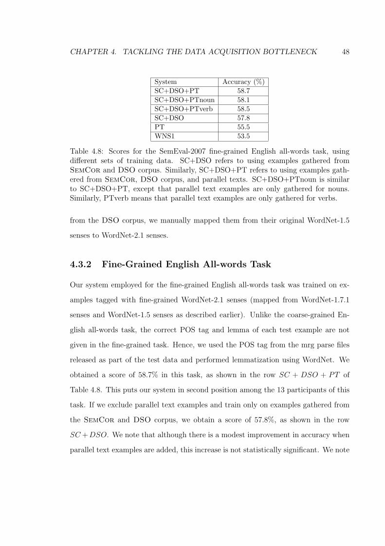
CHAPTER 4. TACKLING THE DATA ACQUISITION BOTTLENECK 48
System Accuracy (%)SC+DSO+PT 58.7SC+DSO+PTnoun 58.1SC+DSO+PTverb 58.5SC+DSO 57.8PT 55.5WNS1 53.5
Table 4.8: Scores for the SemEval-2007 fine-grained English all-words task, usingdifferent sets of training data. SC+DSO refers to using examples gathered fromSemCor and DSO corpus. Similarly, SC+DSO+PT refers to using examples gath-ered from SemCor, DSO corpus, and parallel texts. SC+DSO+PTnoun is similarto SC+DSO+PT, except that parallel text examples are only gathered for nouns.Similarly, PTverb means that parallel text examples are only gathered for verbs.
from the DSO corpus, we manually mapped them from their original WordNet-1.5
senses to WordNet-2.1 senses.
4.3.2 Fine-Grained English All-words Task
Our system employed for the fine-grained English all-words task was trained on ex-
amples tagged with fine-grained WordNet-2.1 senses (mapped from WordNet-1.7.1
senses and WordNet-1.5 senses as described earlier). Unlike the coarse-grained En-
glish all-words task, the correct POS tag and lemma of each test example are not
given in the fine-grained task. Hence, we used the POS tag from the mrg parse files
released as part of the test data and performed lemmatization using WordNet. We
obtained a score of 58.7% in this task, as shown in the row SC + DSO + PT of
Table 4.8. This puts our system in second position among the 13 participants of this
task. If we exclude parallel text examples and train only on examples gathered from
the SemCor and DSO corpus, we obtain a score of 57.8%, as shown in the row
SC +DSO. We note that although there is a modest improvement in accuracy when
parallel text examples are added, this increase is not statistically significant. We note

CHAPTER 4. TACKLING THE DATA ACQUISITION BOTTLENECK 49
System Accuracy (%)SC+DSO+PT 82.5SC+DSO+PTnoun 82.3SC+DSO+PTadj 81.8SC+DSO+PTverb 81.8SC+DSO 81.7PT 80.0WNS1 78.9
Table 4.9: Scores for the SemEval-2007 coarse-grained English all-words task, usingdifferent sets of training data.
Doc-ID No. of Accuracy (%)test examples Our system Task organizers
d001 368 88.3 86.1d002 379 88.1 85.5d003 500 83.4 79.6d004 677 76.1 86.9d005 345 81.4 75.7
Overall 2269 82.5 83.2
Table 4.10: Score of each individual test document, for the SemEval-2007 coarse-grained English all-words task.
that there are only 465 test examples for this fine-grained task (much fewer than the
coarse-grained task), so this test data set may be too small to serve as an effective
evaluation data set.
4.3.3 Coarse-Grained English All-words Task
Our system employed for the coarse-grained English all-words task was trained with
the coarse-grained WordNet-2.1 sense inventory released by the task organizers. For
this task, the POS tag and lemma of each test example are explicitly given by the
task organizers. Our system developed for this task obtained a score of 82.5% in
this task, as shown in the row SC + DSO + PT of Table 4.9. For comparison, the
WordNet first sense baseline score as calculated by the task organizers is 78.9%.

CHAPTER 4. TACKLING THE DATA ACQUISITION BOTTLENECK 50
It turns out that among the 14 participating systems in this task, the UOR-SSI
system developed by one of the task organizers returned the best score of 83.2%. This
system is based on the Structural Semantics Interconnections algorithm (Navigli and
Velardi, 2005). To disambiguate word senses, it uses semantic relations in WordNet,
semantic relations extracted from annotated corpora, and dictionaries of collocations.
Since the score of this system is not considered part of the official scores, our score
puts our system in the first position among the participants of this task. Further,
the task description paper (Navigli, Litkowski, and Hargraves, 2007) reveals that our
system out performed the UOR-SSI system on all test documents except the fourth
document d004. We will describe some investigations into our system’s relatively
poor performance on this document shortly.
To gauge the contribution of parallel text examples, we retrained our system using
only examples gathered from the SemCor and DSO corpus. As shown in the row
SC + DSO of Table 4.9, this gives a score of 81.7% when scored against the answer
keys released by the task organizers. Although adding examples from parallel texts
gives only a modest improvement in score, this improvement is statistically significant
at a p-value ≤ 0.01. Also, we are improving over the very strong baseline of training
on manually annotated examples of the SemCor and DSO corpus. Moreover, we
note that this improvement is achieved from a relatively small set of word types which
are found to be frequently occurring in BC. Future work can explore expanding the
set of word types by automating the process of assigning Chinese translations to each
sense of an English word, with the use of suitable bilingual lexicons. Finally, we
also calculated the contribution of parallel text examples for each individual POS
category of noun (SC +DSO +PTnoun), adjective (SC +DSO +PTadj), and verb
(SC + DSO + PTverb). As shown in Table 4.9, parallel text examples gathered for

CHAPTER 4. TACKLING THE DATA ACQUISITION BOTTLENECK 51
each POS category provided improvement in score.
As part of the evaluation results, the task organizers also released the scores of our
system on each of the 5 test documents. We show in Table 4.10 the total number of
test examples in each document, along with the score we obtained for each document
under the column Our system. We note that our system obtained a relatively low
score on the fourth document, which is a Wikipedia entry on computer programming.
To determine the reason for the low score, we looked through the list of test words
in that document. We noticed that the noun program has 20 test examples occurring
in that fourth document. From the answer keys released by the task organizers, all
20 test examples belong to the sense of “a sequence of instructions that a computer
can interpret and execute”, for which our WSD system does not have any training
examples. Similarly, we noticed that another noun programming has 27 test examples
occurring in the fourth document which belong to the sense of “creating a sequence
of instructions to enable the computer to do something”, for which our WSD system
does not have any training examples. Thus, these two words alone account for 47
of the errors made by our system in this task, representing 2.1% of the 2,269 test
examples of this task. In Table 4.10 under the column Task organizers, we show the
scores obtained by the system developed by the task organizers. This was the best
performing system we had mentioned earlier, but where its score was not considered
part of the official scores. Interestingly, we note that the performance of our WSD
system is better across all test documents, except the fourth one.

CHAPTER 4. TACKLING THE DATA ACQUISITION BOTTLENECK 52
Error type No. of error occurrencesWrong sentence alignment 3Wrong word alignment 11Ambiguous Chinese translation 103Wrong POS tag 11Inappropriate translation in text 9Ambiguous context 16Total 153
Table 4.11: Sense-tag analysis over 1000 examples
4.4 Sense-tag Accuracy of Parallel Text Examples
As part of the SemEval-2007 evaluation exercise, we organized an English lexical
sample task for WSD (Ng and Chan, 2007), where the sense-annotated examples
were gathered from parallel texts. Two tracks were organized for the task, with each
track using a different corpus. For one of the tracks, we used the Sinorama parallel
corpus and measured the annotation accuracy of examples gathered from the corpus.
In this section, we will discuss the different types of annotation errors found in these
examples.
The word alignment output of GIZA++ contains much noise in general (especially
for the low frequency words). However, note that in our approach, we only select the
English word occurrences that align to the selected Chinese translations. Hence, while
the complete set of word alignment output contains much noise, the subset of word
occurrences chosen may still have high quality sense tags.
To investigate the sense-tag accuracy of the training examples gathered from par-
allel texts, we manually inspected a random selection of 100 examples each from 5
nouns and 5 adjectives. These 10 words have an average of 8.6 senses per word in
the WordNet-1.7.1 sense inventory. Our manual inspection reveals the following main
types of sense annotation errors.

CHAPTER 4. TACKLING THE DATA ACQUISITION BOTTLENECK 53
Wrong sentence alignment Due to erroneous sentence segmentation or sentence
alignment, the correct Chinese word that an English word w should align to is not
present in its Chinese sentence counterpart. In this case, word alignment will align
the wrong Chinese word to w.
Wrong word alignment Sometimes, GIZA++ will align an incorrect Chinese
word to an English occurrence. For instance, for the English-Chinese phrase pair
“. . . smile on his face . . . ” and “Á Q G�”, the English word “face” which has
the meaning of “the front of the human head from the forehead to the chin”, should
be aligned to the Chinese word “Á” but is instead wrongly aligned to the Chinese
word “G�”. Since the Chinese word “G�” was assigned as a translation for sense
2 of the noun “face” which has the meaning “the expression on a person’s face”,
this particular occurrence of “face” is wrongly gathered as an example for sense 2.
Another situation of wrong word alignment occurs when the English word occurrence
has no translation in the corresponding Chinese sentence. GIZA++ might then align
the English word w to some Chinese word. If that aligned Chinese word happens
to be one of the assigned translations for w (but belonging to a different sense),
then this will constitute an incorrect example. Wrong word alignment can also occur
when the sentence is too long. GIZA++ imposes a limit on the maximum sentence
length. Sentences longer than this limit will have the corresponding portion pruned
off. Sometimes, the correct Chinese word that an English word w should align to is
in the portion of the sentence that was pruned off. Thus, word alignment will align
the wrong Chinese word to w.
Ambiguous Chinese translation Some Chinese translations assigned are actu-
ally appropriate across multiple senses of a word. For instance, the translation “;
\” is assigned to sense 1 of the adjective simple, which has the meaning “having

CHAPTER 4. TACKLING THE DATA ACQUISITION BOTTLENECK 54
few parts; not complex or complicated or involved”. Examples for the sense as given
by WordNet includes “a simple problem”, “simple mechanisms”, “a simple design”,
etc. However, “;\” is also appropriate for sense 2 of simple, which has the mean-
ing “easy and not involved or complicated”. Hence, some examples gathered via the
Chinese translation “;\” for sense 1 of the adjective simple actually has the easy
meaning of sense 2. Note that this also highlights the fact that WordNet senses are
sometimes too fine-grained, with several senses sharing very similar meaning.
Wrong POS tag We might be wrongly gathering some examples due to POS
tagging errors made by the POS tagger. For instance, some words such as “face” and
“work” can either be a noun or a verb. When a POS tagger wrongly assigns a verb
occurrence of “face” as having a POS tag of noun, and that particular occurrence of
“face” happens to be aligned to a Chinese word which has been chosen as a translation
for one of the senses of the noun “face”, we would wrongly gather that occurrence of
“face” as a training example.
Inappropriate translation in text In the English-Chinese parallel texts that
we are using, we find that some English words are inappropriately translated. For
instance, in the English sentences “At present, he is an assistant professor of archi-
tecture at Chung Yuan Christian University. His experience in the field is rich.”, the
English noun “field” should have the sense 4 meaning of “a branch of knowledge”.
However, the noun “field” is inappropriately translated as “� ” in the Chinese text.
Since the occurrence of “field” was aligned to “� ” by GIZA++ and “� ” was
chosen as a translation for another sense of the noun “field”, an incorrect example
was gathered.
Ambiguous context We are sometimes unable to clearly distinguish the correct
sense of an example. In these situations, we regard the example as wrongly tagged

CHAPTER 4. TACKLING THE DATA ACQUISITION BOTTLENECK 55
to avoid inflating the sense-tag accuracy.
The result of the analysis is shown in Table 4.11. We note that the main source
of errors is the inherent ambiguity of some Chinese translations. The row Wrong
word alignment summarizes the errors incurred due to GIZA++. From these 1,000
examples, we measure a sense annotation accuracy of 84.7%, which compares favor-
ably with the quality of manually sense tagged corpus prepared in SENSEVAL-2
(Kilgarriff, 2001).
4.5 Summary
In order to build a wide-coverage WSD system, tackling the data acquisition bottle-
neck for WSD is crucial. In this chapter, we showed that the approach of gathering
training examples from parallel texts is promising. With manually assigned Chinese
translations, we gathered examples from parallel texts for a set of frequently occurring
nouns, adjectives, and verbs. When evaluated on the SENSEVAL-2 and SENSEVAL-
3 English all-words task using fine-grained scoring, classifiers trained on parallel text
examples always significantly outperformed the strategy of choosing the first sense of
WordNet. For both SENSEVAL-2 and SENSEVAL-3, we showed that parallel text
examples can help to further improve the performance of classifiers trained on the
manually annotated examples of SemCor and DSO.
We also participated in the coarse-grained English all-words task and fine-grained
English all-words task of SemEval-2007. Using training examples gathered from par-
allel texts, SemCor, and the DSO corpus, we trained supervised WSD systems.
Evaluation results showed that this approach achieved good performance in both
tasks.

Chapter 5
Word Sense Disambiguation with
Sense Prior Estimation
Supervised WSD systems that are trained on one domain but applied to another
domain show a decrease in performance, with one major reason being that different
domains have different sense priors. Hence, estimation of sense priors is important
for building widely applicable WSD systems. In (Chan and Ng, 2005b) and (Chan
and Ng, 2006), we used various algorithms to estimate the sense priors in a new text
corpus and showed that they are effective in improving WSD accuracies.
In this chapter, we first describe the various algorithms to estimate the sense pri-
ors. Then, in Section 5.3, we describe the notion of being well calibrated and discuss
why using well calibrated probabilities helps in estimating the sense priors. We also
describe an algorithm to calibrate the probability estimates from naive Bayes. Then
in Section 5.4, we discuss the corpora and the set of words we use for our experiments.
In Section 5.5, we present our experimental results over all the words in our dataset.
In Section 5.6, we describe experiments with using the well calibrated probabilities
56

CHAPTER 5. WSD WITH SENSE PRIOR ESTIMATION 57
of logistic regression to estimate the sense priors. We note that estimation of sense
priors is important when there is a change in domain, usually being reflected by a
change in predominant senses of words. In Section 5.7, we assume we know the true
predominant sense of each word in the training and target domains, and present our
evaluation results over those words having different predominant senses between the
two domains. In a practical setting, however, we do not know the true predominant
sense of each word in a particular domain. In Section 5.8, we predict the predomi-
nant sense of each word and evaluate on those words where the predicted predominant
senses differ between the training and test data. In Section 5.9, we conclude this chap-
ter. Finally, note that for the experiments performed in this chapter, we use the naive
Bayes and logistic regression implementation in WEKA with default parameters.
5.1 Estimation of Priors
To estimate the sense priors, or a priori probabilities of the different senses in a new
data set, we make use of a confusion matrix algorithm (Vucetic and Obradovic, 2001)
or an EM-based algorithm (Saerens, Latinne, and Decaestecker, 2002). In this section,
we describe these two algorithms and the predominant sense method introduced by
McCarthy et al. (2004b).
5.1.1 Confusion Matrix
Let us assume that from a set of labeled data DL, a classifier is used to compute the
conditional probability pL(ωj|ωi) , which is an estimate of the probability of classifying
an instance as class ωj , when in fact it belongs to class ωi . Then, one can apply this
classifier with known conditional probabilities pL(ωj|ωi) to a set of unlabeled data DU

CHAPTER 5. WSD WITH SENSE PRIOR ESTIMATION 58
DL
DtrainDtest
split
DU
classifier
train
bootstrapsample D*test
bootstrapbootstrapsample D*U
bootstrap
p = P-1 · q repeat for B iterations
Figure 5.1: Sense priors estimation using the confusion matrix algorithm.
to obtain its predictions. From these predictions, one can estimate the probability of
predicting class ωj on DU , which we will denote as q(ωj) . The a priori probabilities
p(ωi) on DU (which in our context are the sense priors we want to estimate) are then
estimated by solving the following equation:
q(ωj) =n∑
i=1
pL(ωj|ωi)p(ωi), j = 1, . . . , n (5.1)
where n represents the number of classes. Equation (5.1) can be represented in matrix
form as q = P · p, from which the a priori probabilities on DU , represented by p ,
can be estimated by solving:
p = P−1 · q (5.2)

CHAPTER 5. WSD WITH SENSE PRIOR ESTIMATION 59
To obtain estimates of P and q, bootstrap sampling (Efron and Tibshirani, 1993)
is employed. In bootstrap sampling, given an original sample X with n examples,
bootstrap sample X∗ is obtained by randomly sampling n examples from X with
replacement. To estimate the conditional probabilities pL(ωj|ωi), we need to split
our labeled data DL into Dtrain and Dtest. We will first use Figure 5.1 to provide an
overview of the confusion matrix algorithm before giving the algorithmic details.
As shown in Figure 5.1, we first split DL into Dtrain and Dtest. Then, we generate
a bootstrap sample D∗test from Dtest and apply the classifier trained on Dtrain on D∗
test.
This gives us the conditional probabilities pL(ωj|ωi), or the P matrix. We similarly
generate a bootstrap sample D∗U from DU and apply the same classifier on D∗
U . Using
this classification result, we calculate q(ωj), which is the vector q. Using Equation 5.2,
we then solve for p. We repeat this process of obtaining bootstrap samples D∗test and
D∗U , then calculating the vector p of a priori probabilities, for a total of B iterations.
We then average the vectors p over the B iterations to obtain our final estimate of
the a priori probabilities, or the sense priors of the different senses in the unlabeled
data DU .
Now, we will give the confusion matrix algorithm. We first define n∗test(ωj, ωi) as
the number of examples in a bootstrap sample D∗test predicted to be of class ωj when
the true class is ωi. Also, we define n∗U(ωj) as the number of examples in a bootstrap
sample D∗U predicted to be of class ωj. Then, given Dtest, DU , and a classifier, repeat
the following for B iterations (in our experiments, we set B to 200):
• Generate a bootstrap sample from ntest examples of Dtest and calculate:
p∗L(ωj|ωi) =n∗test(ωj ,ωi)Pj n∗test(ωj ,ωi)
for i, j = 1, . . . , n
• Generate a bootstrap sample from nU examples of DU and calculate:
q∗(ωj) =n∗U (ωj)
nUfor j = 1, . . . , n

CHAPTER 5. WSD WITH SENSE PRIOR ESTIMATION 60
• Use Equation (5.2) to calculate p∗(ωi)(b)for i = 1, . . . , n
After B iterations, estimate the a priori probabilities p(ωi) = 1B
∑Bb=1 p∗(ωi)
(b)
5.1.2 EM-Based Algorithm
Most of this section is based on (Saerens, Latinne, and Decaestecker, 2002), which
introduced the EM-based algorithm1 to estimate the a priori probabilities in a new
corpus. Assume we have a set of labeled data DL with n classes and a set of N
independent instances (x1, . . . ,xN) from a new data set. The likelihood of these N
instances can be defined as:
L(x1, . . . ,xN) =N∏
k=1
p(xk)
=N∏
k=1
[n∑
i=1
p(xk, ωi)
]
=N∏
k=1
[n∑
i=1
p(xk|ωi)p(ωi)
](5.3)
Assuming the within-class densities p(xk|ωi), i.e., the probabilities of observing xk
given the class ωi, do not change from the training set DL to the new data set, we can
define: p(xk|ωi) = pL(xk|ωi). To determine the a priori probability estimates p(ωi) of
the new data set that will maximize the likelihood of (5.3) with respect to p(ωi), we
can apply the iterative procedure of the EM algorithm. In effect, through maximizing
the likelihood of (5.3), we obtain the a priori probability estimates as a by-product.
1A derivation of this algorithm is available in the Appendix section of (Saerens, Latinne, andDecaestecker, 2002).

CHAPTER 5. WSD WITH SENSE PRIOR ESTIMATION 61
Let us now define some notations. When we apply a classifier trained on DL on
an instance xk drawn from the new data set DU , we get pL(ωi|xk), which we define
as the probability of instance xk being classified as class ωi by the classifier trained
on DL. Further, let us define pL(ωi) as the a priori probabilities of class ωi in DL.
This can be estimated by the class frequency of ωi in DL. We also define p(s)(ωi)
and p(s)(ωi|xk) as estimates of the new a priori and a posteriori probabilities at step
s of the iterative EM procedure. Assuming we initialize p(0)(ωi) = pL(ωi), then for
each instance xk in DU and each class ωi, the EM algorithm provides the following
iterative steps:
p(s)(ωi|xk) =pL(ωi|xk)
bp(s)(ωi)bpL(ωi)∑n
j=1 pL(ωj|xk)bp(s)(ωj)
bpL(ωj)
(5.4)
p(s+1)(ωi) =1
N
N∑
k=1
p(s)(ωi|xk) (5.5)
where Equation (5.4) represents the expectation E-step, Equation (5.5) represents the
maximization M-step, and N represents the number of instances in DU . Note that
the probabilities pL(ωi|xk) and pL(ωi) in Equation (5.4) will stay the same through-
out the iterations for each particular instance xk and class ωi. The new a posteriori
probabilities p(s)(ωi|xk) at step s in Equation (5.4) are simply the a posteriori prob-
abilities in the conditions of the labeled data, pL(ωi|xk), weighted by the ratio of the
new priors p(s)(ωi) to the old priors pL(ωi). The denominator in Equation (5.4) is
simply a normalizing factor.
The a posteriori p(s)(ωi|xk) and a priori probabilities p(s)(ωi) are re-estimated
sequentially during each iteration s for each new instance xk and each class ωi, until
the convergence of the estimated probabilities p(s)(ωi). In the context of our work,
these are the sense priors that we want to estimate. This iterative procedure will

CHAPTER 5. WSD WITH SENSE PRIOR ESTIMATION 62
increase the likelihood of (5.3) at each step.
5.1.3 Predominant Sense
A method of automatically ranking WordNet senses to determine the predominant,
or most frequent sense, of a noun in the BNC corpus is presented in (McCarthy et
al., 2004b). Using the method of (Lin, 1998), a thesaurus is first acquired from the
parsed 90 million words of written English from the BNC corpus to provide the k
nearest neighbors to each target noun, along with the distributional similarity score
(dss) between the target noun and its neighbor. The WordNet similarity package
(Pedersen, Patwardhan, and Michelizzi, 2004) is then used to give a WordNet sim-
ilarity measure (wnss), which is used to weigh the contribution that each neighbor
makes to the various senses of the target noun. Through a combination of dss and
wnss, a prevalence score for each sense of the target noun is calculated, from which
the predominant sense of the noun in BNC is determined.
Though the focus of the method is to determine the predominant sense, we could
obtain sense priors estimates by normalizing the prevalence score of each sense. We
implemented this method in order to evaluate its effectiveness in improving WSD
accuracy. Our implementation achieved accuracies close to those reported by Mc-
Carthy et al. (2004b). In that work, the authors reported a jcn measure predominant
sense accuracy of 54.0% on the SemCor corpus, while we measured 53.3% using
our implementation. On the SENSEVAL-2 English all-words task, 64.0% precision
and 63.0% recall were reported. Our implementation gave 66.2% precision and 63.4%
recall. The differences could be due to some minor processing steps which were not
described in detail in (McCarthy et al., 2004b). Finally, note that this predominant
sense method is only effective on a very large text corpus, as the thesaurus can only

CHAPTER 5. WSD WITH SENSE PRIOR ESTIMATION 63
DL : training data
DU : unlabeled evaluation data
NBclassifier
train apply kiLp x|ˆ :posterior
probabilities
EM
ip :estimated sense
priors in DU
iLp :a priori
probabilities in DL
adjust
adjustedposterior
probabilities
Figure 5.2: Sense priors estimation using the EM algorithm.
be effectively generated from a very large corpus.
5.2 Using A Priori Estimates
If a classifier estimates posterior class probabilities pL(ωi|xk) when presented with
a new instance xk from DU , the pL(ωi|xk) probabilities can be directly adjusted
according to the estimated a priori probabilities p(ωi) on DU , thus giving a new set
of class membership predictions.
Denoting predictions of the classifier as pL(ωi|xk), a priori probability of class ωi
from DL as pL(ωi), and estimated a priori probability of class ωi from DU as p(ωi),
adjusted predictions padjust(ωi|xk) can be calculated as:
padjust(ωi|xk) =pL(ωi|xk)
bp(ωi)bpL(ωi)∑
j pL(ωj|xk)bp(ωj)
bpL(ωj)
(5.6)
Figure 5.2 shows the process of estimating and using the sense priors with the EM-
based algorithm. As shown, we first train, for instance a naive Bayes classifier, on the
labeled training data DL. The classifier is then applied on the unlabeled evaluation
CHAPTER 5. WSD WITH SENSE PRIOR ESTIMATION 64
data DU to obtain a set of posterior probability estimates pL(ωi|xk), which are our
initial class membership predictions. Using pL(ωi|xk) and the a priori probabilities
pL(ωi), or proportion of each class in DL, we estimate the sense priors p(ωi) in DU with
the EM-based algorithm using Equation 5.4 and 5.5. These estimated sense priors
p(ωi) can then be used to adjust the initial predictions pL(ωi|xk) using Equation 5.6,
to obtain a new set of class membership predictions padjust(ωi|xk). We will show in
the experimental section later that padjust(ωi|xk) are more accurate than the initial
pL(ωi|xk) predictions.
5.3 Calibration of Probabilities
In our eariler work (Chan and Ng, 2005b), the posterior probabilities assigned by
a naive Bayes classifier are used by the EM procedure described in Section 5.1.2
to estimate the sense priors p(ωi) in a new dataset. However, it is known that the
posterior probabilities assigned by naive Bayes are not well calibrated (Domingos and
Pazzani, 1996).
It is important to use an algorithm which gives well calibrated probabilities, if we
are to use the probabilities in estimating the sense priors. In this section, we will
first describe the notion of being well calibrated before discussing why having well
calibrated probabilities helps in estimating the sense priors. Finally, we will introduce
a method used to calibrate the probabilities.
5.3.1 Well Calibrated Probabilities
Assume for each instance x, a classifier outputs a probability Sωi(x) between 0 and
1, of x belonging to class ωi. The classifier is well-calibrated if the empirical class

CHAPTER 5. WSD WITH SENSE PRIOR ESTIMATION 65
membership probability p(ωi|Sωi(x) = t) converges to the probability value Sωi
(x) = t
as the number of examples classified goes to infinity (Zadrozny and Elkan, 2002).
Intuitively, if we consider all the instances to which the classifier assigns a probability
Sωi(x) of say 0.6, then 60% of these instances should be members of class ωi.
5.3.2 Being Well Calibrated Helps Estimation
To see why using an algorithm which gives well calibrated probabilities helps in esti-
mating the sense priors, let us rewrite Equation (5.5), the M-step of the EM procedure,
as the following:
p(s+1)(ωi) =1
N
∑t∈Swi
∑
k∈{q:Sωi (xq)=t}p(s)(ωi|xk) (5.7)
where Sωi= {t1, . . . , tm} denotes the set of posterior probability values for class ωi,
and Sωi(xq) denotes the posterior probability of class ωi assigned by the classifier for
instance xq.
Based on t1, . . . , tm, we can imagine that we have m bins, where each bin is
associated with a specific t value. Now, distribute all the instances in the new dataset
DU into the m bins according to their posterior probabilities Sωi(x). Let Bl, for
l = 1, . . . ,m, denote the set of instances in bin l.
Note that |B1| + · · · + |Bl| + · · · + |Bm| = N . Now, let pl denote the proportion
of instances with true class label ωi in Bl. Given a well calibrated algorithm, pl = tl

CHAPTER 5. WSD WITH SENSE PRIOR ESTIMATION 66
by definition and Equation (5.7) can be rewritten as:
p(s+1)(ωi) =1
N(t1|B1|+ · · ·+ tm|Bm|)
=1
N(p1|B1|+ · · ·+ pm|Bm|)
=Nωi
N(5.8)
where Nωidenotes the number of instances in DU with true class label ωi. Therefore,
p(s+1)(ωi) reflects the proportion of instances in DU with true class label ωi. Hence,
using an algorithm which gives well calibrated probabilities helps in the estimation
of sense priors.
5.3.3 Isotonic Regression
Zadrozny and Elkan (2002) successfully used a method based on isotonic regression
(Robertson, Wright, and Dykstra, 1988) to calibrate the probability estimates from
naive Bayes. To compute the isotonic regression, they used the pair-adjacent violators
(PAV) (Ayer et al., 1955) algorithm, which we show in Figure 5.3. Briefly, what PAV
does is to initially view each data value as a level set. While there are two adjacent
sets that are out of order (i.e., the left level set is above the right one) then the sets
are combined and the mean of the data values becomes the value of the new level set.
PAV works on binary class problems. In a binary class problem, we have a posi-
tive class and a negative class. Now, let D = (pk,xk), 1 ≤ k ≤ N , where x1, . . . ,xN
represent N examples and pk is the probability of xk belonging to the positive class,
as predicted by a classifier. Further, let yk represent the true label of xk. For a binary
class problem, we let yk = 1 if xk is a positive example and yk = 0 if xk is a negative
example. The PAV algorithm takes in a set of (pk, yk), sorted in ascending order of pk

CHAPTER 5. WSD WITH SENSE PRIOR ESTIMATION 67
Input: training set (pk, yk) sorted in ascending order of pk
Initialize gk = yk
While ∃ k such that gj, . . . , gk−1 > gk, . . . , gl, where gj = · · · = gk−1 andgk = · · · = gl (j < k ≤ l)
Set m =Pl
q=j gq
l−j+1
Replace gj, . . . , gl with m
Figure 5.3: PAV algorithm.
training data: classes ‘+’, ‘ ’
validation data x1: (p1, y1) … xk: (pk, yk) … xN: (pN, yN)
classifier train apply
Sort the set of (pk,yk) in increasing order of pk :
Sorted p values:0.1 0.2 0.3 0.4 0.5 0.6 0.7 0.8 0.9 1.0
Corresponding y values: 0 0 1 0 1 0 0 1 1 1
0 0 0.5 0.5 1 0 0 1 1 1
0 0 0.5 0.5 0.33 0.33 0.33 1 1 1
0 0 0.4 0.4 0.4 0.4 0.4 1 1 1
Calibration mapping: 0.1 0.2 0.3 0.4 0.5 0.6 0.7 0.8 0.9 1.0
0 0 0.4 0.4 0.4 0.4 0.4 1 1 1
Figure 5.4: PAV illustration.

CHAPTER 5. WSD WITH SENSE PRIOR ESTIMATION 68
and returns a series of increasing step-values, where each step-value gj,l (denoted by
m in Figure 5.3) is associated with a lowest boundary value pj and a highest boundary
value pl. We performed 10-fold cross-validation on the training data to assign values
to pk. We then applied the PAV algorithm to obtain values for gk. To obtain the
calibrated probability estimate for a test instance x, we find the boundary values pj
and pl where pj ≤ Sωi(x) ≤ pl and assign gj,l as the calibrated probability estimate.
As an illustration of the PAV algorithm, let us refer to Figure 5.4. After training
our classifier on the binary class training data, we apply it on our validation data to
obtain a set D = (pk,xk), 1 ≤ k ≤ N . Similarly, we let yk represent the true label of xk
and sort the set of (pk, yk) in ascending order of pk. Assume we have N=10 validation
instances, their sorted p values are 0.1, 0.2, . . . , 1.0; and their corresponding y values
are as shown in the figure: 0 0 1 0 1 0 0 1 1 1. Note that if the prediction probabilities
pk had ranked the instances perfectly, all the 0’s will come before all the 1’s and we
would have “0 0 0 0 0 1 1 1 1 1”. Starting from the first, or leftmost y value, the PAV
algorithm searches for any occurrence where a y value is greater than the value on its
right. In essence, the PAV algorithm will try to smooth out the series of y values. In
our example given in Figure 5.4, the PAV algorithm detects that y3 (with a value of
1) is greater than y4 (with a value of 0). The average of these 2 numbers is computed,
resulting in the second series of values: 0 0 0.5 0.5 1 0 0 1 1 1. The PAV algorithm
now detects that the 3 underlined numbers (1 0 0) are “out of order”. Their average
value is computed and we have the third series of numbers: 0 0 0.5 0.5 0.33 0.33 0.33
1 1 1. Finally, the algorithm detects that the 5 underlined numbers (0.5 0.5 0.33 0.33
0.33) are “out of order” and averages them, resulting in the last series of numbers: 0
0 0.4 0.4 0.4 0.4 0.4 1 1 1. Since all numbers are now in increasing order, the PAV
algorithm ends its execution and we have obtained the calibration mapping, which is

CHAPTER 5. WSD WITH SENSE PRIOR ESTIMATION 69
just a mapping between numbers. For this example, our mapping indicates that if our
original probability estimate pk of belonging to the positive class is 0 ≤ pk ≤ 0.2, the
new estimate is 0; if 0.3 ≤ pk ≤ 0.7, the new estimate is 0.4, etc. If pk falls between
two boundary values, such as if 0.2 < pk < 0.3, we average the associated calibrated
probabilities to obtain (0 + 0.4)/2 = 0.2.
To apply PAV on a multiclass problem, we first reduce the problem into a number
of binary class problems. For reducing a multiclass problem into a set of binary
class problems, experiments in (Zadrozny and Elkan, 2002) suggest that the one-
against-all approach works well. In one-against-all, a separate classifier is trained for
each class ωi, where examples belonging to class ωi are treated as positive examples
and all other examples are treated as negative examples. A separate classifier is
then learnt for each binary class problem and the probability estimates from each
classifier are calibrated. Finally, the calibrated binary-class probability estimates are
combined to obtain multiclass probabilities, computed by a simple normalization of
the calibrated estimates from the binary classifiers, as suggested by Zadrozny and
Elkan (2002). For instance, assume a particular problem consists of 4 classes and
their calibrated binary-class probabilities are 0.2, 0.3, 0.3, and 0.5. To normalize
these probabilities, we first compute their total (0.2 + 0.3 + 0.3 + 0.5) = 1.3 and then
divide each probability by the total. This gives the normalized calibrated probabilities
0.2/1.3 = 0.15, 0.3/1.3 = 0.23, etc.
5.4 Selection of Dataset
In this section, we discuss the motivations in choosing the particular corpora and the
set of words used in our experiments.

CHAPTER 5. WSD WITH SENSE PRIOR ESTIMATION 70
5.4.1 DSO Corpus
The DSO corpus is made up of texts drawn from Brown corpus (BC) and Wall Street
Journal (WSJ). BC is a balanced corpus and contains texts in various categories such
as religion, fiction, etc. In contrast, the focus of the WSJ corpus is on financial
and business news. Escudero, Marquez, and Rigau (2000) exploited the difference in
coverage between these two corpora to separate the DSO corpus into its BC and WSJ
parts for investigating the domain dependence of several WSD algorithms. Following
their setup, we also use the DSO corpus in our experiments. Since BC is a balanced
corpus, and training a classifier on a general corpus before applying it to a more
specific corpus is a natural scenario, we use examples from the BC portion of DSO
as training data, and examples from the WSJ portion of DSO as evaluation data, or
the target dataset.
5.4.2 Parallel Texts
To build a wide-coverage WSD system, we require a large amount of training exam-
ples. In Chapter 4, we have shown that parallel texts provide an effective source for
gathering these examples. However, note that the parallel texts we use (as given in
Table 4.1) are gathered from different sources such as legislative proceedings, mag-
azine articles, etc. Hence, examples gathered from parallel texts typically present a
natural domain difference from the target data on which we apply the WSD system.
In particular, we note that since the test data of the English lexical sample task in
SENSEVAL-2 and SENSEVAL-3 is largely drawn from the British National corpus
(BNC), this represents a domain difference from the parallel text examples. Hence,
we include a set of experiments where we train on parallel text examples and eval-
uate on the nouns of SENSEVAL-2 and SENSEVAL-3 English lexical sample task.

CHAPTER 5. WSD WITH SENSE PRIOR ESTIMATION 71
Dataset Total no. of words No. different PS No. same PSDSO nouns 119 37 82DSO verbs 66 28 38SE2 nouns 15 6 9SE3 nouns 17 9 8
Table 5.1: Number of words with different or the same predominant sense (PS) be-tween the training and test data.
Following (Ng, Wang, and Chan, 2003), in gathering examples from parallel texts,
senses will be lumped together if they are translated in the same way in Chinese.
5.5 Results Over All Words
We first present our experimental results over all the words of our test data, no matter
whether they have different or the same predominant sense between the training and
test data.
As mentioned earlier, the DSO corpus contains annotated examples for 121 nouns
and 70 verbs. After leaving out the few nouns and verbs which have only BC examples
and no WSJ examples in the DSO corpus, we are left with a set of 119 nouns and
66 verbs, as shown in Table 5.1. Among these words, 37 nouns and 28 verbs have
different predominant senses between the training data (BC portion of DSO) and
test data (WSJ portion of DSO). For the remaining 82 nouns and 38 verbs as shown
under the column No. same PS of Table 5.1, their respective predominant sense
remains unchanged between the BC and WSJ portion of the DSO corpus.
For the nouns of SENSEVAL-2 and SENSEVAL-3 English lexical sample tasks,
we do not perform WSD on 7 SENSEVAL-2 nouns that are lumped into one sense
(i.e., all the senses of each of these nouns were translated into the same Chinese

CHAPTER 5. WSD WITH SENSE PRIOR ESTIMATION 72
Classifier NBMethod L True CMNB EMNB EMLogR
DSO nouns 64.0 67.9 64.5 64.7 64.6DSO verbs 58.1 62.3 58.8 58.9 59.0SE2 nouns 70.5 72.2 70.8 70.8 71.3SE3 nouns 62.1 63.6 63.0 62.8 63.0
Table 5.2: Micro-averaged WSD accuracies over all the words, using the variousmethods. The naive Bayes here are multiclass naive Bayes (NB).
Classifier NBMethod True − L CMNB − L EMNB − L EMLogR − LDSO nouns 3.9 0.5 (12.8%) 0.7 (17.9%) 0.6 (15.4%)DSO verbs 4.2 0.7 (16.7%) 0.8 (19.0%) 0.9 (21.4%)SE2 nouns 1.7 0.3 (17.6%) 0.3 (17.6%) 0.8 (47.1%)SE3 nouns 1.5 0.9 (60.0%) 0.7 (46.7%) 0.9 (60.0%)
Table 5.3: Relative accuracy improvement based on non-calibrated probabilities.
word). In (Saerens, Latinne, and Decaestecker, 2002) which introduced the EM-based
algorithm, experiments were conducted using a minimum of 50 training examples for
each class. In our current work, we use a similar but less restrictive criterion of
omitting those words with less than 50 examples. This omitted 7 SENSEVAL-2
nouns and 3 SENSEVAL-3 nouns as they have less than 50 parallel text examples
available. Thus, we are left with a set of 15 SENSEVAL-2 nouns and 17 SENSEVAL-3
nouns, as shown under the column Total no. of words in Table 5.1. For each noun,
we gathered a maximum of 500 parallel text examples as training data, similar to
what we had done in (Chan and Ng, 2005b).

CHAPTER 5. WSD WITH SENSE PRIOR ESTIMATION 73
5.5.1 Experimental Results
We now present experimental results on the set of words listed under the column
Total no. of words in Table 5.1. We used the supervised WSD system described in
Chapter 3 with naive Bayes as our learning algorithm. All accuracies reported in our
experiments are micro-averages over the test examples.
We record the WSD accuracies achieved by a multiclass naive Bayes classifier
(without any adjustment), in the column L under NB in Table 5.2. For the EM-based
algorithm, the predictions pL(ωi|xk) of these naive Bayes classifiers are then used in
Equation (5.4) and (5.5) to estimate the sense priors p(ωi), before being adjusted by
these estimated sense priors based on Equation (5.6). The resulting WSD accuracies
after this adjustment are listed in the column EMNB in Table 5.2. For instance, in
Table 5.2 we see that for the set of DSO verbs, we obtained a WSD accuracy of
58.1% using the original predictions of the naive Bayes classifier. If we adjust these
predictions by the sense priors estimated via the EM-based algorithm, performance
improves to 58.9%.
Corresponding WSD accuracies achieved from adjusting the original predictions
pL(ωi|xk) by the sense priors estimated by the confusion matrix algorithm are listed
under the column CMNB. To provide a basis for comparison, we also adjusted the
predictions pL(ωi|xk) by the true sense priors p(ωi) of the test data. The accuracies
thus obtained are shown under the column True in Table 5.2.
The increases in WSD accuracies obtained through using the estimated sense
priors are given in Table 5.3 (the numbers in this table are derived from Table 5.2).
The column True − L in the table shows the increase in WSD accuracy obtained by
using the true sense priors of the test data. Note that this represents the maximum
possible increase in accuracy achievable provided we know these true sense priors

CHAPTER 5. WSD WITH SENSE PRIOR ESTIMATION 74
p(ωi). In the column EMNB − L in Table 5.3, we list the increase in WSD accuracy
when the naive Bayes predictions are adjusted by the sense priors p(ωi) which are
automatically estimated using the EM procedure. The relative improvements obtained
with using the estimated sense priors p(ωi), as compared against using the true sense
priors p(ωi), are given as percentages in brackets. For instance, for the set of DSO
verbs, adjusting the original predictions by the sense priors estimated via the EM
algorithm gives an improvement of 0.8% in accuracy, against an improvement of 4.2%
if we were to use the true sense priors. Thus, the relative improvement is 0.8/4.2 =
19%. Corresponding figures of relative improvements based on using sense priors
estimated by the confusion matrix algorithm are given under the column CMNB −L.
In Section 5.1.3, we mentioned that we could normalize the prevalence score of
each sense to obtain estimated sense priors via the predominant sense method. We
note that the thesaurus used as part of the predominant sense method is acquired
from the BNC corpus, from which the majority of the SENSEVAL-2 and SENSEVAL-
3 English lexical sample task test data are drawn. Hence, we applied the sense priors
estimated via the predominant sense method on our test data of SENSEVAL-2 and
SENSEVAL-3 nouns, obtaining an accuracy of 70.6% and 62.6%, respectively. Note
that these are lower than the scores obtained via the confusion matrix algorithm and
EM-based algorithm, consistent with the findings in (Chan and Ng, 2005b). This
suggests that in a supervised setting where training data is available, the confusion
matrix and EM-based algorithms estimate the sense priors more effectively than the
unsupervised predominant sense method. The predominant sense method also has
the drawback that it is only able to estimate the sense priors, or predominant sense,
in a very large text corpus, which is needed to construct the thesaurus. In contrast,
the confusion matrix algorithm is applicable on texts of any size. For the EM-based

CHAPTER 5. WSD WITH SENSE PRIOR ESTIMATION 75
DL : training data
DU : unlabeled evaluation data
NBclassifier
train apply kiLp x|ˆ :posterior
probabilities
EM
ip :estimated sense
priors in DU
iLp :a priori
probabilities in DL
kiLp x|ˆ :calibratedposterior
probabilities
calibrate
adjustedcalibratedposterior
probabilities
adjust
Figure 5.5: Sense priors estimation using the EM algorithm with calibration.
algorithm, experiments in (Saerens, Latinne, and Decaestecker, 2002) show that the
size of the target corpus has little effect on its effectiveness.
Next, we used the one-against-all approach to reduce each multiclass problem into
a set of binary class problems. We trained a naive Bayes classifier for each binary
class problem and calibrated the probabilities from these binary classifiers. The WSD
accuracies of these calibrated naive Bayes classifiers (denoted by NBcal) are given in
the column L under NBcal of Table 5.4. The predictions of these classifiers are then
used to estimate the sense priors p(ωi), before being adjusted by these estimates
based on Equation (5.6). Figure 5.5 gives an overview of the process when using the
calibrated probabilities to estimate the sense priors via the EM-based algorithm. Note
the similarity with Figure 5.2. The difference is that we calibrate the probabilities
before providing them to the EM algorithm and that these are in turn adjusted by
the estimated sense priors. The resulting WSD accuracies after adjustment are listed
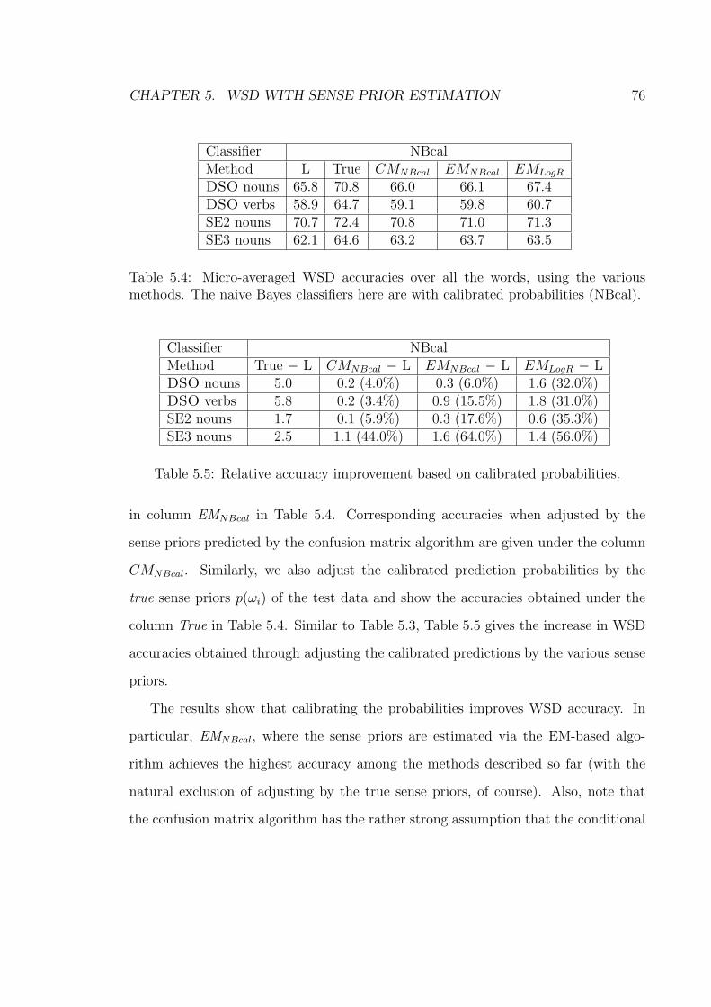
CHAPTER 5. WSD WITH SENSE PRIOR ESTIMATION 76
Classifier NBcalMethod L True CMNBcal EMNBcal EMLogR
DSO nouns 65.8 70.8 66.0 66.1 67.4DSO verbs 58.9 64.7 59.1 59.8 60.7SE2 nouns 70.7 72.4 70.8 71.0 71.3SE3 nouns 62.1 64.6 63.2 63.7 63.5
Table 5.4: Micro-averaged WSD accuracies over all the words, using the variousmethods. The naive Bayes classifiers here are with calibrated probabilities (NBcal).
Classifier NBcalMethod True − L CMNBcal − L EMNBcal − L EMLogR − LDSO nouns 5.0 0.2 (4.0%) 0.3 (6.0%) 1.6 (32.0%)DSO verbs 5.8 0.2 (3.4%) 0.9 (15.5%) 1.8 (31.0%)SE2 nouns 1.7 0.1 (5.9%) 0.3 (17.6%) 0.6 (35.3%)SE3 nouns 2.5 1.1 (44.0%) 1.6 (64.0%) 1.4 (56.0%)
Table 5.5: Relative accuracy improvement based on calibrated probabilities.
in column EMNBcal in Table 5.4. Corresponding accuracies when adjusted by the
sense priors predicted by the confusion matrix algorithm are given under the column
CMNBcal. Similarly, we also adjust the calibrated prediction probabilities by the
true sense priors p(ωi) of the test data and show the accuracies obtained under the
column True in Table 5.4. Similar to Table 5.3, Table 5.5 gives the increase in WSD
accuracies obtained through adjusting the calibrated predictions by the various sense
priors.
The results show that calibrating the probabilities improves WSD accuracy. In
particular, EMNBcal, where the sense priors are estimated via the EM-based algo-
rithm achieves the highest accuracy among the methods described so far (with the
natural exclusion of adjusting by the true sense priors, of course). Also, note that
the confusion matrix algorithm has the rather strong assumption that the conditional

CHAPTER 5. WSD WITH SENSE PRIOR ESTIMATION 77
probabilities pL(ωj|ωi) stay the same from the training or labeled data DL, to the test
or unlabeled data DU on which we want to estimate the sense priors. Furthermore,
the method also involves the time consuming process of performing many additional
classification runs, such as multiple bootstrap samplings and cross-validations to cal-
culate matrices P and vectors q. In contrast, the EM-based method does not require
any additional experimental runs. To estimate the sense priors using the EM-based
method, we only need to iteratively perform the two EM steps of Equation (5.4) and
(5.5). In view of these considerations, we focus on using the EM-based algorithm to
estimate the sense priors for the rest of our experiments in this chapter.
5.6 Sense Priors Estimation with Logistic Regres-
sion
The experimental results show that the sense priors estimated using the calibrated
probabilities of naive Bayes are effective in increasing the WSD accuracy. However,
using a learning algorithm which already gives well calibrated posterior probabilities
may be more effective in estimating the sense priors. One possible algorithm is
logistic regression, which directly optimizes for getting approximations of the posterior
probabilities. Hence, its probability estimates are already well calibrated (Zhang and
Yang, 2004; Niculescu-Mizil and Caruana, 2005).
We trained logistic regression classifiers and evaluated them on the set of words
of the four datasets. However, the WSD accuracies of these unadjusted logistic re-
gression classifiers are on average lower than those of the unadjusted naive Bayes
classifiers. One possible reason is that being a discriminative learner, logistic regres-
sion requires more training examples for its performance to catch up to, and possibly

CHAPTER 5. WSD WITH SENSE PRIOR ESTIMATION 78
DL : training
data DU : unlabeled
evaluation data
NB
classifier
train apply ( )kiLp x|� :
posterior
probabilities
( )kiLp x|� :
calibrated
posterior
probabilities
calibrate
DL : training
dataDU : unlabeled
evaluation data
Logistic
regression
classifier
train apply ( )kiLp x|� :
posterior
probabilities
EM
( )ip� :
estimated sense
priors in DU
( )iLp� :
a priori
probabilities in DL
adjust
�NBcal EM logR�:
adjusted
calibrated
posterior
probabilities
�NB EM logR�:
adjusted
posterior
probabilities
Figure 5.6: Sense priors estimation with logistic regression.
even overtake, the generative naive Bayes learner (Ng and Jordan, 2001).
Although the accuracy of logistic regression as a basic classifier is lower than that
of naive Bayes, its predictions may still be suitable for estimating sense priors. These
sense priors could then be used to adjust the prediction probabilities of the naive
Bayes classifiers. Figure 5.6 gives an overview of the process. Notice that the top
half of the figure is very similar to Figure 5.2, except that the naive Bayes classifier
is replaced by the logistic regression classifier.
To elaborate on Figure 5.6, we first train a logistic regression classifier on the
labeled training data DL. The classifier is then applied on the unlabeled evaluation
data DU to obtain a set of posterior probability estimates pL(ωi|xk), which are our

CHAPTER 5. WSD WITH SENSE PRIOR ESTIMATION 79
initial class membership predictions. Using pL(ωi|xk) and the a priori probabilities
pL(ωi), or proportion of each class in DL, we estimate the sense priors p(ωi) in DU
with the EM-based algorithm using Equation 5.4 and 5.5. The steps described up till
now are exactly the same as those in Figure 5.2, except that the naive Bayes classifier
is replaced by the logistic regression classifier. As a result, we have computed the
sense priors estimated by logistic regression.
As shown in the lower half of Figure 5.6, we now train naive Bayes classifers
on DL and apply them on DU , to obtain an initial set of naive Bayes predictions
pL(ωi|xk). We then either apply (using Equation (5.6)) the sense priors estimated
earlier by logistic regression on these naive Bayes prediction probabilities to obtain
a set of adjusted predictions “NB EMlogR”, or we can calibrate the original naive
Bayes predictions before applying the sense priors to obtain “NBcal EMlogR”.
The WSD accuracy of “NB EMlogR” (the predictions pL(ωi|xk) of the uncalibrated
naive Bayes adjusted by the sense priors estimated with logistic regression) is given
in the column EMLogR under NB of Table 5.2. Corresponding WSD accuracies of
“NBcal EMlogR” (the predictions pL(ωi|xk) of the calibrated naive Bayes adjusted by
the sense priors estimated with logistic regression) is given in the column EMLogR
under NBcal of Table 5.4. The relative improvements over using the true sense pri-
ors, based on the uncalibrated and calibrated probabilities, are given in the column
EMLogR − L of Table 5.3 and Table 5.5, respectively. The results show that the sense
priors estimated with logistic regression are in general effective in further improving
the WSD accuracies.

CHAPTER 5. WSD WITH SENSE PRIOR ESTIMATION 80
5.7 Experiments Using True Predominant Sense
Information
Research by (McCarthy et al., 2004b) highlighted that the sense priors of a word
in a corpus depend on the domain from which the corpus is drawn. A change of
predominant sense is often indicative of a change in domain, as different corpora
drawn from different domains usually give different predominant senses. For example,
the predominant sense of the noun interest in the Brown corpus (BC) part of the
DSO corpus has the meaning “a sense of concern with and curiosity about someone
or something”. In the Wall Street Journal (WSJ) part of the DSO corpus, the
noun interest has a different predominant sense with the meaning “a fixed charge for
borrowing money”, reflecting the business and finance focus of the WSJ corpus.
Estimation of sense priors is important when there is a significant change in sense
priors between the training and target dataset, such as when there is a change in
domain between the datasets. In this section, we focus on experiments involving
words having different predominant senses between the training and test data. In our
experiments involving the DSO corpus, we focus on the set of nouns and verbs which
have different predominant senses between the BC and WSJ parts of the corpus. This
gives us a set of 37 nouns and 28 verbs, as tabulated in Table 5.1. For experiments
involving the nouns of SENSEVAL-2 and SENSEVAL-3 English lexical sample task,
we focus on the set of nouns having different predominant senses between the examples
gathered from parallel texts and the evaluation data for the two SENSEVAL tasks.
This gives a set of 6 nouns for SENSEVAL-2 and 9 nouns for SENSEVAL-3, as
tabulated in Table 5.1.

CHAPTER 5. WSD WITH SENSE PRIOR ESTIMATION 81
Classifier NB NBcalMethod L True EMNB EMLogR L True EMNBcal EMLogR
DSO nouns 44.5 51.9 46.1 46.6 45.8 57.4 47.0 51.1DSO verbs 46.7 53.9 48.3 48.7 46.9 57.2 49.5 50.8SE2 nouns 61.7 64.4 62.4 63.0 62.3 65.3 63.2 63.5SE3 nouns 53.9 56.6 54.9 55.7 55.4 59.1 58.8 58.4
Table 5.6: Micro-averaged WSD accuracies using the various methods, for the set ofwords having different predominant senses between the training and test data. Thedifferent naive Bayes classifiers are: multiclass naive Bayes (NB) and naive Bayeswith calibrated probabilities (NBcal).
Dataset True − L EMNB − L EMLogR − LDSO nouns 7.4 1.6 (21.6%) 2.1 (28.4%)DSO verbs 7.2 1.6 (22.2%) 2.0 (27.8%)SE2 nouns 2.7 0.7 (25.9%) 1.3 (48.1%)SE3 nouns 2.7 1.0 (37.0%) 1.8 (66.7%)
Table 5.7: Relative accuracy improvement based on uncalibrated probabilities.
Dataset True − L EMNBcal − L EMLogR − LDSO nouns 11.6 1.2 (10.3%) 5.3 (45.7%)DSO verbs 10.3 2.6 (25.2%) 3.9 (37.9%)SE2 nouns 3.0 0.9 (30.0%) 1.2 (40.0%)SE3 nouns 3.7 3.4 (91.9%) 3.0 (81.1%)
Table 5.8: Relative accuracy improvement based on calibrated probabilities.
Method comparison DSO DSO SE2 SE3nouns verbs nouns nouns
NB EMLogR vs. NB EMNB (add logR) À À À ÀNBcal EMNBcal vs. NB EMNB (add cal) ∼ À > ÀNBcal EMNBcal vs. NB EMLogR (cal vs. logR) ∼ À ∼ ÀNBcal EMLogR vs. NB EMNB (add logR and cal) À À À ÀNBcal EMLogR vs. NB EMLogR (add cal) À À ∼ ÀNBcal EMLogR vs. NBcal EMNBcal (add logR) À À ∼ ∼
Table 5.9: Paired t-tests between the various methods for the four datasets. Here,logistic regression is abbreviated as logR and calibration as cal.

CHAPTER 5. WSD WITH SENSE PRIOR ESTIMATION 82
From the results given in Table 5.6, we see that calibrating the probabilities im-
proves WSD accuracy and using the sense priors estimated by logistic regression is
effective in improving the results. In the case of DSO nouns, the improvement due
to the use of logistic regression is especially significant; from 45.8% to 51.1%. Similar
to the previous section, we show in Table 5.7 and 5.8 the increase in WSD accuracy
from using the automatically estimated sense priors p(wi), as compared to using the
true sense priors p(wi).
Paired t-tests were conducted to see if one method is significantly better than
another. The t statistic of the difference between each test instance pair is computed,
giving rise to a p value. The results of significance tests for the various methods
on the four datasets are given in Table 5.9, where the symbols “∼”, “>”, and “À”
correspond to p-value > 0.05, (0.01, 0.05], and ≤ 0.01 respectively.
The methods in Table 5.9 are represented in the form a1 a2, where a1 denotes
adjusting the predictions of which classifier, and a2 denotes how the sense priors are
estimated. As an example, NBcal EMLogR specifies that the sense priors estimated
by logistic regression are used to adjust the predictions of the calibrated naive Bayes
classifier, and corresponds to accuracies in column EMLogR under NBcal in Table 5.6.
NB EMNB represents our earlier approach in (Chan and Ng, 2005b). The signif-
icance tests show that the approach of using calibrated naive Bayes probabilities to
estimate sense priors, and then adjusting the calibrated probabilities by these sense
priors estimates (NBcal EMNBcal) is more effective than NB EMNB (refer to row 2 of
Table 5.9). For DSO nouns, though the results are similar, the p value is a relatively
low 0.06.
Using sense priors estimated by logistic regression further improves performance.
For example, row 1 of Table 5.9 shows that adjusting the predictions of multiclass

CHAPTER 5. WSD WITH SENSE PRIOR ESTIMATION 83
naive Bayes classifiers by sense priors estimated by logistic regression (NB EMLogR)
performs significantly better than using sense priors estimated by multiclass naive
Bayes (NB EMNB). Finally, using sense priors estimated by logistic regression to
adjust the predictions of calibrated naive Bayes (NBcal EMLogR) in general performs
significantly better than most other methods, achieving the best overall performance.
5.8 Experiments Using Predicted Predominant Sense
Information
Results from the previous section show that it is critical and effective to adjust the
predictions of words having different predominant senses between the training and
test data. However, in a practical setting, we do not know the true predominant sense
of each word in a particular domain or dataset. In this section, we use the EM-based
algorithm to estimate the sense priors in the test data. The sense with the highest
estimated sense prior is taken as the predominant sense of the word.
Similar to Table 5.1, we show in Table 5.10 the number of words having different,
or the same predominant sense, for the four datasets. In addition, each number in
brackets gives the number of words where the EM-based algorithm predicts that there
is a change in predominant sense. For instance, for the 37 DSO nouns having different
predominant senses between the training and test data, the EM-based algorithm is
able to correctly predict that the predominant sense changes for 25 of the nouns.
Similarly for the 82 DSO nouns where their predominant sense remains unchanged
between the training and test data, the EM-based algorithm is able to correctly
predict that there is no change in predominant sense for 81 of the nouns (i.e., it
incorrectly predicts that one noun has its predominant sense changed). This means

CHAPTER 5. WSD WITH SENSE PRIOR ESTIMATION 84
Dataset Total no. of words No. different PS No. same PSDSO nouns 119 (26) 37 (25) 82 (1)DSO verbs 66 (20) 28 (19) 38 (1)SE2 nouns 15 (6) 6 (4) 9 (2)SE3 nouns 17 (6) 9 (5) 8 (1)Total 217 (58) 80 (53) 137 (5)
Table 5.10: Number of words with different or the same predominant sense (PS)between the training and test data. Numbers in brackets give the number of wordswhere the EM-based algorithm predicts a change in predominant sense.
Classifier NB NBcalMethod L True EMNB EMLogR L True EMNBcal EMLogR
DSO nouns 47.5 55.4 49.6 50.0 48.5 60.1 48.9 54.0DSO verbs 49.8 58.1 51.7 52.4 50.9 60.2 53.6 55.9SE2 nouns 67.5 69.8 67.9 68.8 67.4 70.0 67.9 68.7SE3 nouns 55.8 61.5 58.4 59.2 57.2 64.6 64.2 62.9
Table 5.11: Micro-averaged WSD accuracies over the words with predicted differentpredominant senses between the training and test data.
Dataset True − L EMNB − L EMLogR − LDSO nouns 7.9 2.1 (26.6%) 2.5 (31.6%)DSO verbs 8.3 1.9 (22.9%) 2.6 (31.3%)SE2 nouns 2.3 0.4 (17.4%) 1.3 (56.5%)SE3 nouns 5.7 2.6 (45.6%) 3.4 (59.6%)
Table 5.12: Relative accuracy improvement based on uncalibrated probabilities.
Dataset True − L EMNBcal − L EMLogR − LDSO nouns 11.6 0.4 (3.4%) 5.5 (47.4%)DSO verbs 9.3 2.7 (29.0%) 5.0 (53.8%)SE2 nouns 2.6 0.5 (19.2%) 1.3 (50.0%)SE3 nouns 7.4 7.0 (94.6%) 5.7 (77.0%)
Table 5.13: Relative accuracy improvement based on calibrated probabilities.

CHAPTER 5. WSD WITH SENSE PRIOR ESTIMATION 85
that the algorithm predicts that 26 (25+1) DSO nouns have different predominant
senses between the training and test data.
We then evaluate over the set of 58 words where the EM-based algorithm predicts
a change in predominant sense between the training and test data. The improvements
in WSD accuracy from adjusting the predictions using the estimated sense priors for
these words are shown in Table 5.11. The relative improvements based on uncali-
brated and calibrated probabilities are shown in Tables 5.12 and 5.13, respectively.
The results show that in a practical setting where one does not know whether pre-
dominant senses of words changes between the training and test data, one can still
estimate and use the sense priors to improve WSD accuracy. Finally, we note that
the best results are obtained using the sense priors estimated by logistic regression.
5.9 Summary
Differences in sense priors between training and target domain datasets will result
in a loss of WSD accuracy. In this chapter, we show that using well calibrated
probabilities to estimate sense priors is important. By calibrating the probabilities
of the naive Bayes algorithm, and using the probabilities given by logistic regression
(which are already well calibrated), we achieve improvements in WSD accuracy. We
also highlight the importance of estimating the sense priors when there is a change in
domain, which could be reflected by a change in predominant sense. We show that
the EM-based algorithm is effective in predicting a change in predominant sense.
Evaluation over the set of words where the predominant senses between the training
and test data are predicted to be different shows that the EM-based algorithm is able
to predict the sense priors effectively to improve WSD accuracy. Finally, using logistic

CHAPTER 5. WSD WITH SENSE PRIOR ESTIMATION 86
regression to estimate the sense priors via the EM-based algorithm gives consistently
good improvements to WSD accuracy.
Chapter 6
Domain Adaptation with Active
Learning for Word Sense
Disambiguation
We have already highlighted the importance of performing domain adaptation for
WSD. In this chapter, we explore domain adaptation of WSD systems by adding
training examples from the new domain, as additional training data to a WSD system.
To reduce the effort required to adapt a WSD system to a new domain, we employ
an active learning strategy (Lewis and Gale, 1994) to select examples to annotate
from the new domain of interest. To our knowledge, our work is the first to use
active learning for domain adaptation for WSD. A similar work is the recent research
by Chen et al. (2006), where active learning was used successfully to reduce the
annotation effort for WSD of 5 English verbs using coarse-grained evaluation. In that
work, the authors only used active learning to reduce the annotation effort and did
not deal with the porting of a WSD system to a new domain.
87

CHAPTER 6. DOMAIN ADAPTATION WITH ACTIVE LEARNING 88
Domain adaptation is necessary when the training and target domains are differ-
ent. In our work, we perform domain adaptation for WSD of a set of nouns using
fine-grained evaluation. The contribution of our work is not only in showing that
active learning can be successfully employed to reduce the annotation effort required
for domain adaptation in a fine-grained WSD setting. More importantly, our main
focus and contribution is in showing how we can improve the effectiveness of a basic
active learning approach when it is used for domain adaptation. In particular, we
explore the issue of different sense priors across different domains. Using the sense
priors estimated by expectation-maximization (EM), the predominant sense in the
new domain is predicted. Using this predicted predominant sense and adopting a
count-merging technique, we improve the effectiveness of the adaptation process.
In the next section, we discuss the choice of corpus and nouns used in our ex-
periments. We then introduce active learning for domain adaptation, followed by
count-merging. Performance of domain adaptation using active learning and count-
merging is then presented. Next, we show that by using the predominant sense of the
target domain as predicted by the EM-based algorithm, we improve the effectiveness
of the adaptation process. Our empirical results show that for the set of nouns which
have different predominant senses between the training and target domains, we are
able to reduce the annotation effort by 71%.
6.1 Experimental Setting
For the experiments performed in this chapter, we use the naive Bayes implementation
in WEKA as our learning algorithm. In this section, we discuss the motivations for
choosing the particular corpus and the set of nouns to conduct our domain adaptation

CHAPTER 6. DOMAIN ADAPTATION WITH ACTIVE LEARNING 89
experiments.
6.1.1 Choice of Corpus
Similar to the last chapter, we made use of the DSO corpus to perform our experiments
on domain adaptation. The DSO corpus has two parts: Brown corpus (BC) and the
Wall Street Journal (WSJ). Since BC is a balanced corpus, and since performing
adaptation from a general corpus to a more specific corpus is a natural scenario, we
focus on adapting a WSD system trained on BC to WSJ. Henceforth, out-of-domain
data will refer to BC examples, and in-domain data will refer to WSJ examples.
6.1.2 Choice of Nouns
The WordNet Domains resource (Magnini and Cavaglia, 2000) assigns domain labels
to synsets in WordNet. Since the focus of the WSJ corpus is on business and financial
news, we can make use of WordNet Domains to select the set of nouns having at least
one synset labeled with a business or finance related domain label. This is similar
to the approach taken in (Koeling, McCarthy, and Carroll, 2005) where they focus
on determining the predominant sense of words in corpora drawn from finance versus
sports domains.1 Hence, we select the subset of DSO nouns that have at least one
synset labeled with any of these domain labels: commerce, enterprise, money, finance,
banking, and economy. This gives a set of 21 nouns: book, business, center, community,
condition, field, figure, house, interest, land, line, money, need, number, order, part,
power, society, term, use, value.2
1Note however that the coverage of the WordNet Domains resource is not comprehensive, asabout 31% of the synsets are simply labeled with “factotum”, indicating that the synset does notbelong to a specific domain.
225 nouns have at least one synset labeled with the listed domain labels. In our experiments, 4out of these 25 nouns have an accuracy of more than 90% before adaptation (i.e., training on just

CHAPTER 6. DOMAIN ADAPTATION WITH ACTIVE LEARNING 90
Dataset No. of MFS No. of No. ofsenses accuracy training adaptation
BC WSJ (%) examples examples21 nouns 6.7 6.8 61.1 310 4069 nouns 7.9 8.6 65.8 276 416
Table 6.1: The average number of senses in BC and WSJ, average MFS accuracy,average number of BC training, and WSJ adaptation examples per noun.
For each noun, all the BC examples are used as out-of-domain training data. One-
third of the WSJ examples for each noun are set aside as evaluation data, and the
rest of the WSJ examples are designated as in-domain adaptation data. The row 21
nouns in Table 6.1 shows some information about these 21 nouns. For instance, these
nouns have an average of 6.7 senses in BC and 6.8 senses in WSJ. This is slightly
higher than the 5.8 senses per verb in (Chen et al., 2006), where the experiments were
conducted using coarse-grained evaluation. Assuming we had access to an “oracle”
which determines the predominant sense, or the most frequent sense (MFS), of each
noun in our WSJ test data perfectly, and we assign this most frequent sense to each
noun in the test data, we would have achieved an accuracy of 61.1% as shown in the
column MFS accuracy of Table 6.1. Finally, we note that we have an average of 310
BC training examples and 406 WSJ adaptation examples per noun.
6.2 Active Learning
For our experiments, we use the WSD system described in Chapter 3 with naive
Bayes as the learning algorithm. In our domain adaptation study, we start with
a WSD system built using training examples drawn from BC. We then investigate
the BC examples) and accuracy improvement is less than 1% after all the available WSJ adaptationexamples are added as additional training data. To obtain a clearer picture of the adaptation process,we discard these 4 nouns, leaving a set of 21 nouns.

CHAPTER 6. DOMAIN ADAPTATION WITH ACTIVE LEARNING 91
DT ← the set of BC training examplesDA ← the set of untagged WSJ adaptation examplesΓ ← WSD system trained on DT
repeatpmin ← ∞for each d ∈ DA do
s ← word sense prediction for d using Γp ← confidence of prediction sif p < pmin then
pmin ← p, dmin ← dend
endDA ← DA − dmin
provide correct sense s for dmin and add dmin to DT
Γ ← WSD system trained on new DT
end
Figure 6.1: Active learning
the utility of adding additional in-domain training data from WSJ. In the baseline
approach, the additional WSJ examples are randomly selected. With active learning
(Lewis and Gale, 1994), we use uncertainty sampling as shown in Figure 6.1. In each
iteration, we train a WSD system on the available training data and apply it on the
WSJ adaptation examples. Among these WSJ examples, the example predicted with
the lowest confidence is selected and removed from the adaptation data. The correct
label is then supplied for this example and it is added to the training data.
Note that in the experiments reported in this chapter, all the adaptation examples
are already pre-annotated before the experiments start, since all the WSJ adapta-
tion examples come from the DSO corpus which have already been sense-annotated.
Hence, the annotation of an example needed during each adaptation iteration is sim-
ulated by performing a lookup without any manual annotation.

CHAPTER 6. DOMAIN ADAPTATION WITH ACTIVE LEARNING 92
6.3 Count-merging
We also employ a technique known as count-merging in our domain adaptation
study. Count-merging assigns different weights to different examples to better re-
flect their relative importance. Roark and Bacchiani (2003) showed that weighted
count-merging is a special case of maximum a posteriori (MAP) estimation, and suc-
cessfully used it for probabilistic context-free grammar domain adaptation (Roark
and Bacchiani, 2003) and language model adaptation (Bacchiani and Roark, 2003).
Count-merging can be regarded as scaling of counts obtained from different data
sets. We let c denote the counts from out-of-domain training data, c denote the
counts from in-domain adaptation data, and p denote the probability estimate by
count-merging. We can scale the out-of-domain and in-domain counts with different
factors, or just use a single weight parameter β:
p(fj|si) =c(fj, si) + βc(fj, si)
c(si) + βc(si)(6.1)
Similarly,
p(si) =c(si) + βc(si)
c + βc(6.2)
Obtaining an optimum value for β is not the focus of this work. Instead, we are
interested to see if assigning a higher weight to the in-domain WSJ adaptation ex-
amples, as compared to the out-of-domain BC examples, will improve the adaptation
process. Hence, we just use a β value of 3 in our experiments involving count-merging.

CHAPTER 6. DOMAIN ADAPTATION WITH ACTIVE LEARNING 93
52
54
56
58
60
62
64
66
68
70
72
74
76
0 5 10 15 20 25 30 35 40 45 50 55 60 65 70 75 80 85 90 95 100
WS
D A
ccur
acy
(%)
Percentage of adaptation examples added (%)
a-car
a-truePrior
Figure 6.2: Adaptation process for all 21 nouns. In the graph, the curves are: r(random selection), a (active learning), a-c (active learning with count-merging), a-truePrior (active learning, with BC examples gathered to adhere to true sense priorsin WSJ).
6.4 Experimental Results
For each adaptation experiment, we start off with a classifier built from an initial
training set consisting of the BC training examples. At each adaptation iteration,
WSJ adaptation examples are selected one at a time and added to the training set.
The adaptation process continues until all the adaptation examples are added. Clas-
sification accuracies averaged over 3 random trials on the WSJ test examples at each
iteration are calculated. Since the number of WSJ adaptation examples differs for

CHAPTER 6. DOMAIN ADAPTATION WITH ACTIVE LEARNING 94
each of the 21 nouns, the learning curves we will show in the various figures are plot-
ted in terms of different percentage of adaptation examples added, varying from 0
to 100 percent in steps of 1 percent. To obtain these curves, we first calculate for
each noun, the WSD accuracy when different percentages of adaptation examples are
added. Then, for each percentage, we calculate the macro-average WSD accuracy
over all the nouns to obtain a single learning curve representing all the nouns.
6.4.1 Utility of Active Learning and Count-merging
In Figure 6.2, the curve r represents the adaptation process of the baseline approach,
where additional WSJ examples are randomly selected during each adaptation iter-
ation. The adaptation process using active learning is represented by the curve a,
while applying count-merging with active learning is represented by the curve a-c.
Note that random selection r achieves its highest WSD accuracy after all the adap-
tation examples are added. To reach the same accuracy, the a approach requires the
addition of only 57% of adaptation examples. The a-c approach is even more effective
and requires only 42% of adaptation examples. This demonstrates the effectiveness
of count-merging in further reducing the annotation effort, when compared to using
only active learning. To reach the MFS accuracy of 61.1% as shown earlier in Table
6.1, a-c requires just 4% of the adaptation examples.
6.4.2 Using Sense Priors Information
As mentioned previously, research in (Escudero, Marquez, and Rigau, 2000) noted an
improvement in accuracy when they adjusted the BC and WSJ datasets such that
the proportions of the different senses of each word were the same between BC and
WSJ. We can similarly choose BC examples such that the sense priors in the BC

CHAPTER 6. DOMAIN ADAPTATION WITH ACTIVE LEARNING 95
training data adhere to the sense priors in the WSJ evaluation data. To gauge the
effectiveness of this approach, we first assume that we know the true sense priors of
each noun in the WSJ evaluation data. We then gather BC training examples for a
noun to adhere as much as possible to the sense priors in WSJ. Assume sense si is
the predominant sense in the WSJ evaluation data, and si has a sense prior of pi in
the WSJ data and has ni BC training examples. Taking ni examples to represent a
sense prior of pi, we proportionally determine the number of BC examples to gather
for the other senses according to their respective sense priors in WSJ. If there are
insufficient training examples in BC for some sense s, whatever available examples of
s are used.
This approach gives an average of 195 BC training examples for the 21 nouns.
With this new set of training examples, we perform adaptation using active learning
and obtain the a-truePrior curve in Figure 6.2. The a-truePrior curve shows that by
ensuring that the sense priors in the BC training data adhere as much as possible to
the sense priors in the WSJ data, we start off with a higher WSD accuracy. However,
the performance is no different from the a curve after 35% of adaptation examples
are added. A possible reason might be that by strictly adhering to the sense priors
in the WSJ data, we have removed too many BC training examples, from an average
of 310 examples per noun as shown in Table 6.1 to an average of 195 examples.
6.4.3 Using Predominant Sense Information
Research by McCarthy et al. (2004b) and Koeling, McCarthy, and Carroll (2005)
pointed out that a change of predominant sense is often indicative of a change in
domain. For example, the predominant sense of the noun interest in the BC part
of the DSO corpus has the meaning “a sense of concern with and curiosity about

CHAPTER 6. DOMAIN ADAPTATION WITH ACTIVE LEARNING 96
someone or something”. In the WSJ part of the DSO corpus, the noun interest has a
different predominant sense with the meaning “a fixed charge for borrowing money”,
which is reflective of the business and finance focus of the WSJ corpus.
Instead of restricting the BC training data to adhere strictly to the sense priors
in WSJ, another alternative is just to ensure that the predominant sense in BC is the
same as that of WSJ. Out of the 21 nouns, 12 nouns have the same predominant sense
in both BC and WSJ. The remaining 9 nouns that have different predominant senses
in the BC and WSJ data are: center, field, figure, interest, line, need, order, term,
value. The row 9 nouns in Table 6.1 gives some information for this set of 9 nouns.
To gauge the utility of this approach, we conduct experiments on these nouns by first
assuming that we know the true predominant sense in the WSJ data. Assume that
the WSJ predominant sense of a noun is si and si has ni examples in the BC data.
We then gather BC examples for a noun to adhere to this WSJ predominant sense,
by gathering only up to ni BC examples for each sense of this noun. This approach
gives an average of 190 BC examples for the 9 nouns. This is higher than an average
of 83 BC examples for these 9 nouns if BC examples are selected to follow the sense
priors of WSJ evaluation data as described in the last subsection 6.4.2.
For these 9 nouns, the average KL-divergence between the sense priors of the
original BC data and WSJ evaluation data is 0.81. This drops to 0.51 after ensuring
that the predominant sense in BC is the same as that of WSJ, confirming that the
sense priors in the newly gathered BC data more closely follow the sense priors in WSJ.
Using this new set of training examples, we perform domain adaptation using active
learning to obtain the curve a-truePred in Figure 6.3. For comparison, we also plot
the curves a and a-truePrior for this set of 9 nouns in Figure 6.3. Results in Figure
6.3 show that a-truePred starts off at a higher accuracy and performs consistently

CHAPTER 6. DOMAIN ADAPTATION WITH ACTIVE LEARNING 97
43 44 45 46 47 48 49 50 51 52 53 54 55 56 57 58 59 60 61 62 63 64 65 66 67 68 69 70 71 72 73 74 75 76 77 78 79 80 81 82
0 5 10 15 20 25 30 35 40 45 50 55 60 65 70 75 80 85 90 95 100
WS
D A
ccur
acy
(%)
Percentage of adaptation examples added (%)
a-truePriora-truePred
a
Figure 6.3: Using true predominant sense for the 9 nouns. The curves are: a (activelearning), a-truePrior (active learning, with BC examples gathered to adhere to truesense priors in WSJ), a-truePred (active learning, with BC examples gathered suchthat its predominant sense is the same as the true predominant sense in WSJ).
better than the a curve. In contrast, though a-truePrior starts at a high accuracy,
its performance is lower than a-truePred and a after 50% of adaptation examples
have been added. The approach represented by a-truePred is a compromise between
ensuring that the sense priors in the training data follow as closely as possible the
sense priors in the evaluation data, while retaining enough training examples. These
results highlight the importance of striking a balance between these two goals.
In Section 5.1.3, we described the method presented in (McCarthy et al., 2004b),
where the aim is to determine the predominant sense of a word in a corpus. We have
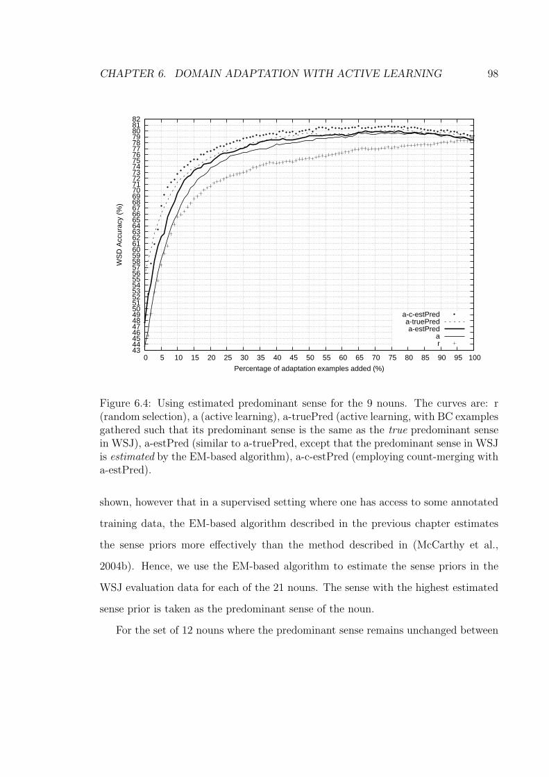
CHAPTER 6. DOMAIN ADAPTATION WITH ACTIVE LEARNING 98
43 44 45 46 47 48 49 50 51 52 53 54 55 56 57 58 59 60 61 62 63 64 65 66 67 68 69 70 71 72 73 74 75 76 77 78 79 80 81 82
0 5 10 15 20 25 30 35 40 45 50 55 60 65 70 75 80 85 90 95 100
WS
D A
ccur
acy
(%)
Percentage of adaptation examples added (%)
a-c-estPreda-truePreda-estPred
ar
Figure 6.4: Using estimated predominant sense for the 9 nouns. The curves are: r(random selection), a (active learning), a-truePred (active learning, with BC examplesgathered such that its predominant sense is the same as the true predominant sensein WSJ), a-estPred (similar to a-truePred, except that the predominant sense in WSJis estimated by the EM-based algorithm), a-c-estPred (employing count-merging witha-estPred).
shown, however that in a supervised setting where one has access to some annotated
training data, the EM-based algorithm described in the previous chapter estimates
the sense priors more effectively than the method described in (McCarthy et al.,
2004b). Hence, we use the EM-based algorithm to estimate the sense priors in the
WSJ evaluation data for each of the 21 nouns. The sense with the highest estimated
sense prior is taken as the predominant sense of the noun.
For the set of 12 nouns where the predominant sense remains unchanged between

CHAPTER 6. DOMAIN ADAPTATION WITH ACTIVE LEARNING 99
Accuracy % adaptation examples neededr a a-estPred a-c-estPred
50%: 61.1 8 7 (0.88) 5 (0.63) 4 (0.50)60%: 64.5 10 9 (0.90) 7 (0.70) 5 (0.50)70%: 68.0 15 12 (0.80) 9 (0.60) 6 (0.40)80%: 71.5 23 16 (0.70) 12 (0.52) 9 (0.39)90%: 74.9 46 24 (0.52) 21 (0.46) 15 (0.33)100%: 78.4 100 51 (0.51) 38 (0.38) 29 (0.29)
Table 6.2: Annotation savings and percentage of adaptation examples needed to reachvarious accuracies.
BC and WSJ, the EM-based algorithm is able to predict that the predominant sense
remains unchanged for all 12 nouns. Hence, we will focus on the 9 nouns which have
different predominant senses between BC and WSJ for our remaining adaptation
experiments. For these 9 nouns, the EM-based algorithm correctly predicts the WSJ
predominant sense for 6 nouns. Hence, the algorithm is able to predict the correct
predominant sense for 18 out of 21 nouns overall, representing an accuracy of 86%.
Figure 6.4 plots the curve a-estPred, which is similar to a-truePred, except that
the predominant sense is now estimated by the EM-based algorithm. Employing
count-merging with a-estPred produces the curve a-c-estPred. For comparison, the
curves r, a, and a-truePred are also plotted. The results show that a-estPred performs
consistently better than a, and a-c-estPred in turn performs better than a-estPred.
Hence, employing the predicted predominant sense and count-merging, we further
improve the effectiveness of the active learning-based adaptation process.
With reference to Figure 6.4, the WSD accuracies of the r and a curves before
and after adaptation are 43.7% and 78.4% respectively. Starting from the mid-point
61.1% accuracy, which represents a 50% accuracy increase from 43.7%, we show in
Table 6.2 the percentage of adaptation examples required by the various approaches
to reach certain levels of WSD accuracies. For instance, to reach the final accuracy

CHAPTER 6. DOMAIN ADAPTATION WITH ACTIVE LEARNING 100
of 78.4%, r, a, a-estPred, and a-c-estPred require the addition of 100%, 51%, 38%,
and 29% adaptation examples respectively. The numbers in brackets give the ratio
of adaptation examples needed by a, a-estPred, and a-c-estPred versus random se-
lection r. For instance, to reach a WSD accuracy of 78.4%, a-c-estPred needs only
29% adaptation examples, representing a ratio of 0.29 and an annotation saving of
71%. Note that this represents a more effective adaptation process than the basic
active learning a approach, which requires 51% adaptation examples. Hence, besides
showing that active learning can be used to reduce the annotation effort required
for domain adaptation, we have further improved the effectiveness of the adaptation
process by using the predicted predominant sense of the new domain and adopting
the count-merging technique.
6.5 Summary
Domain adaptation is important to ensure the general applicability of WSD systems
across different domains. In this chapter, we have shown that active learning is
effective in reducing the annotation effort required in porting a WSD system to a new
domain. Also, we have successfully used an EM-based algorithm to detect a change
in predominant sense between the training and new domain. With this information
on the predominant sense of the new domain and incorporating count-merging, we
have shown that we are able to improve the effectiveness of the original adaptation
process achieved by the basic active learning approach.

Chapter 7
Word Sense Disambiguation for
Machine Translation
Recent research presents conflicting evidence on whether WSD systems can help to
improve the performance of statistical machine translation (MT) systems. In this
chapter, we show how we successfully integrate a state-of-the-art WSD system into
the state-of-the-art hierarchical phrase-based MT system, Hiero. We show for the first
time that integrating a WSD system improves the performance of a state-of-the-art
statistical MT system on an actual translation task. Furthermore, the improvement
is statistically significant.
We start the chapter by describing the Hiero MT system and introducing the two
new features used to integrate the WSD system into Hiero. We then describe the
training data used by the WSD system. Following that, we describe how the WSD
translations provided are used by the decoder of the Hiero MT system. Then, we
present and analyze our experimental results, before concluding the chapter.
101

CHAPTER 7. WSD FOR MT 102
7.1 Hiero
Hiero (Chiang, 2005) is a hierarchical phrase-based model for statistical machine
translation, based on weighted synchronous context-free grammar (CFG) (Lewis and
Stearns, 1968). A synchronous CFG consists of rewrite rules such as the following:
X→ 〈γ, α〉 (7.1)
where X is a non-terminal symbol, and each of γ and α is a string of terminal and
non-terminal symbols in the source and target language, respectively. There is a
one-to-one correspondence between the non-terminals in γ and α indicated by co-
indexation. Hence, γ and α always have the same number of non-terminal symbols.
For instance, we could have the following grammar rule:
X→ 〈�Ût X1
, go to X1
every month to〉 (7.2)
where boxed indices represent the correspondences between non-terminal symbols.
Hiero extracts the synchronous CFG rules automatically from a word-aligned par-
allel corpus. One can treat a rule as a mapping, or as a translation. For instance, the
above rule indicates that we will translate the phrase “� Û t X1
” as “go to
X1
every month to”.
To translate a source sentence, the goal is to find its most probable derivation
using the extracted grammar rules. For instance, assume that c1 . . . c9 in Figure 7.1
represents a Chinese source sentence with 9 words. To translate this source sentence,
Hiero attempts to use the extracted grammar rules to find a suitable derivation that
spans the sentence.

CHAPTER 7. WSD FOR MT 103
,
,c8X1
c7c5 c9
c4
c3 c6
c2
c1
,XX 21
,
1
1
2X X
X
,,
,
,
1X
c1 c2 c3 c4 c5 c6 c7 c8 c9
Figure 7.1: An example derivation which consists of 8 grammar rules. The sourcestring of each rule is represented by the box before the comma, while the shadedboxes represent the target strings of the rules.
Hiero uses a general log-linear model (Och and Ney, 2002) where the weight of a
derivation D for a particular source sentence and its translation is
w(D) =∏
i
φi(D)λi (7.3)
where φi is a feature function and λi is the weight for feature φi. To ensure efficient
decoding, the φi are subject to certain locality restrictions. Essentially, they should be
defined as products of functions defined on isolated synchronous CFG rules. However,
it is possible to extend the domain of locality of the features somewhat. For instance,
an n-gram language model adds a dependence on (n−1) neighboring target-side words
(Wu, 1996; Chiang, 2007), making decoding much more difficult but still polynomial.
In our work, we add features that depend on the neighboring source-side words,

CHAPTER 7. WSD FOR MT 104
which does not affect decoding complexity at all because the source string is fixed.
In principle we could add features that depend on arbitrary source-side context.
7.1.1 New Features in Hiero for WSD
To incorporate WSD into Hiero, we use the translations proposed by the WSD system
to help Hiero obtain a better or more probable derivation during the translation of
each source sentence. To achieve this, when a grammar rule R is considered during
decoding, and we recognize that some of the terminal symbols (words) in α are also
chosen by the WSD system as translations for some terminal symbols (words) in γ,
we compute the following features:
• Pwsd(t | s) gives the contextual probability of the WSD classifier choosing t
as a translation for s, where t (s) is some substring of terminal symbols in α
(γ). Because this probability only applies to some rules, and we don’t want to
penalize those rules, we must add another feature,
• Ptywsd = exp(−|t|), where t is the translation chosen by the WSD system. This
feature, with a negative weight, rewards rules that use translations suggested
by the WSD module.
Note that we can take the negative logarithm of the rule/derivation weights and
think of them as costs rather than probabilities. If we do this, then to translate
a source sentence, our goal will be to find the derivation with the least cost. To
illustrate, consider Figure 7.1. The cost of a derivation depends on the rules that
make up the derivation. The cost of a rule, in turn, consists of the costs contributed
by features defined on the rule. Hence to translate a source sentence, Hiero tries
different rules to find the derivation with the least cost. Now, assume that Hiero

CHAPTER 7. WSD FOR MT 105
,c7c5
c4 ,X1
… c3 c4 c5 c6 c7 …
,
Figure 7.2: We perform WSD on the source string “c5”, using the derived contextdependent probability to change the original cost of the grammar rule.
has determined that for the source sentence c1 . . . c9, the derivation in Figure 7.1
is the one with the least cost. Since each rule represents rewriting its source string
as its target string, the target strings of the rule (represented by the shaded boxes)
actually give the translation of the source sentence c1 . . . c9. This means that once
a particular grammar rule is used as part of the best derivation, its target string will
be part of the translated output. This ties in to the main idea of how we use WSD
to improve Hiero’s translation.
To illustrate further, Figure 7.2 highlights the grammar rule with the source string
“c5”. This rule is part of the derivation shown in Figure 7.1. When the grammar rule
is included as part of the derivation, the source string “c5” will be translated into
the rule’s target string, represented by the shaded box. We want to know whether
our WSD system supports this translation. Hence we perform WSD on the source
string “c5”, given its surrounding context, to determine what is the context dependent
probability of the source string “c5” translating into the target string represented by
the shaded box. This information is used to change the original cost of this grammar
rule, and this is done for every rule. Hence, we use the WSD system to change
the costs of the grammar rules, where the change in costs is dependent upon the
contextual probability of the rule’s source string translating into its target string. We
CHAPTER 7. WSD FOR MT 106
hope this will help Hiero obtain a more informed derivation and thus produce a better
translation.
7.2 Gathering Training Examples for WSD
Our experiments were for Chinese to English translation. Hence, in the context of
our work, a synchronous CFG grammar rule X → 〈γ, α〉 gathered by Hiero consists
of a Chinese portion γ and a corresponding English portion α, where each portion is
a sequence of words and non-terminal symbols.
Our WSD classifier suggests a list of English phrases (where each phrase consists
of one or more English words) with associated contextual probabilities as possible
translations for each particular Chinese phrase. In general, the Chinese phrase may
consist of k Chinese words, where k = 1, 2, 3, . . .. However, we limit k to 1 or 2 for
experiments reported here. Future work can explore enlarging k.
Whenever Hiero is about to extract a grammar rule where its Chinese portion
is a phrase of one or two Chinese words with no non-terminal symbols, we note the
location (sentence and token offset) in the Chinese half of the parallel corpus from
which the Chinese portion of the rule is extracted. The actual sentence in the corpus
containing the Chinese phrase, and the one sentence before and the one sentence
after that actual sentence, will serve as the context for one training example for the
Chinese phrase, with the corresponding English phrase of the grammar rule as its
translation, or “sense class”. Hence, unlike traditional WSD where the sense classes
are tied to a specific sense inventory, our “senses” here consist of the target strings
of grammar rules, which in the context of our work are English phrases extracted as
translations for each Chinese phrase. This is similar to the multilingual lexical sample

CHAPTER 7. WSD FOR MT 107
task of SENSEVAL-3 (Chklovski et al., 2004) and Task 11 (English lexical sample
task via English-Chinese parallel text) of SemEval-2007, where sense distinctions are
decided by the use of different translations in the target language. Since the extracted
training data may be noisy, for each Chinese phrase, we remove English translations
that occur only once. Furthermore, we only attempt WSD classification for those
Chinese phrases with at least 10 training examples.
Using the WSD classifier described in Section 3.2.2, which uses the LIBSVM
implementation of SVM as its learning algorithm, we classified the words in each
Chinese source sentence to be translated. We first performed POS-tagging on the
Chinese texts using the tagger of (Ng and Low, 2004). Then, we performed WSD on
all single Chinese words which are tagged as either noun, verb, or adjective. Next,
we classified the Chinese phrases consisting of 2 consecutive Chinese words by simply
treating the phrase as a single unit. When performing classification, we give as output
the set of English translations with associated context-dependent probabilities, which
are the probabilities of a Chinese word (phrase) translating into each English phrase,
depending on the context of the Chinese word (phrase). After WSD, the ith word ci
in every Chinese sentence may have up to 3 sets of associated translations provided
by the WSD system: a set of translations for ci as a single word, a second set of
translations for ci−1ci considered as a single unit, and a third set of translations for
cici+1 considered as a single unit.
7.3 Incorporating WSD during Decoding
The following tasks are performed for each rule that is considered during decoding:
• identify Chinese words to suggest translations for

CHAPTER 7. WSD FOR MT 108
Input: rule R considered during decoding with its own associated costRLc = list of symbols in Chinese portion of RWSDcost = 0i = 1while i ≤ len(Lc):
ci = ith symbol in Lc
if ci is a Chinese word (i.e., not a non-terminal symbol):// seenChunk is a global variable and is passed by reference to matchWSDseenChunk = ∅if (ci is not the last symbol in Lc) and (ci+1 is a terminal symbol):
then ci+1=(i+1)th symbol in Lc, else ci+1 = NULLif (ci+1!=NULL) and (ci, ci+1) as a single unit has WSD translations:
WSDc = set of WSD translations for (ci,ci+1) as a single unitwith context-dependent probabilities
WSDcost = WSDcost + matchWSD(ci, WSDc, seenChunk)WSDcost = WSDcost + matchWSD(ci+1, WSDc, seenChunk)i = i + 1
else:WSDc = set of WSD translations for ci with context-dependent probabilitiesWSDcost = WSDcost + matchWSD(ci, WSDc, seenChunk)
i = i + 1costR = costR + WSDcost
matchWSD(c, WSDc, seenChunk):// seenChunk is the set of chunks of R already examined for possible matching WSD translationscost = 0ChunkSet = set of chunks in R aligned to cfor chunkj in ChunkSet:
if chunkj not in seenChunk:seenChunk = seenChunk ∪ { chunkj }Echunkj = set of English words in chunkj aligned to cCandidatewsd = ∅for wsdk in WSDc:
if (wsdk is sub-sequence of chunkj) and (wsdk contains at least one word in Echunkj ):Candidatewsd = Candidatewsd ∪ { wsdk }
wsdbest = best matching translation in Candidatewsd against chunkj
// costByWSDfeatures sums up the cost of the two WSD featurescost = cost + costByWSDfeatures(wsdbest)
return cost
Figure 7.3: WSD translations affecting the cost of a rule R considered during decod-ing.

CHAPTER 7. WSD FOR MT 109
• match suggested translations against the English side of the rule
• compute features for the rule
The WSD system is able to predict translations only for a subset of Chinese words
or phrases. Hence, we must first identify which parts of the Chinese side of the rule
have suggested translations available. Here, we consider substrings of length up to
two, and we give priority to longer substrings.
Next, we want to know, for each Chinese substring considered, whether the WSD
system supports the Chinese-English translation represented by the rule. If the rule
is finally chosen as part of the best derivation for translating the Chinese sentence,
then all the words in the English side of the rule will appear in the translated English
sentence. Hence, we need to match the translations suggested by the WSD system
against the English side of the rule. It is for these matching rules that the WSD
features will apply.
The translations proposed by the WSD system may be more than one word long.
In order for a proposed translation to match the rule, we require two conditions.
First, the proposed translation must be a substring of the English side of the rule.
For example, the proposed translation “every to” would not match the string “every
month to”. Second, the match must contain at least one aligned Chinese-English
word pair, but we do not make any other requirements about the alignment of the
other Chinese or English words.1 If there are multiple possible matches, we choose the
longest proposed translation; in the case of a tie, we choose the proposed translation
with the highest score according to the WSD model.
1In order to check this requirement, we extended Hiero to make word alignment informationavailable to the decoder.

CHAPTER 7. WSD FOR MT 110
Define a chunk of a rule to be a maximal substring of terminal symbols on the
English side of the rule. For instance, in Rule (7.2), the chunks would be “go to”
and “every month to”. Whenever we find a matching WSD translation, we mark the
whole chunk on the English side as consumed.
Finally, we compute the feature values for the rule. The feature Pwsd(t | s) is the
sum of the costs (according to the WSD model) of all the matched translations, and
the feature Ptywsd is the sum of the lengths of all the matched translations.
Figure 7.3 shows the pseudocode for the rule scoring algorithm in more detail,
particularly with regards to resolving conflicts between overlapping matches. To
illustrate the algorithm given in Figure 7.3, consider Rule (7.2). Hereafter, we will
use symbols to represent the Chinese and English words in the rule: c1, c2, and c3 will
represent the Chinese words “�”, “Û”, and “t” respectively. Similarly, e1, e2, e3,
e4, and e5 will represent the English words go, to, every, month, and to respectively.
Hence, Rule (7.2) has two chunks: e1e2 and e3e4e5. When the rule is extracted from
the parallel corpus, it has these alignments between the words of its Chinese and
English portion: {c1–e3,c2–e4,c3–e1,c3–e2,c3–e5}, which means that c1 is aligned to e3,
c2 is aligned to e4, and c3 is aligned to e1, e2, and e5. Although all words are aligned
here, in general for a rule, some of its Chinese or English words may not be associated
with any alignments.
In our experiment, c1c2 as a phrase has a list of translations proposed by the
WSD system, including the English phrase “every month”. matchWSD will first be
invoked for c1, which is aligned to only one chunk e3e4e5 via its alignment with e3.
Since “every month” is a sub-sequence of the chunk and also contains the word e3
(“every”), it is noted as a candidate translation. Later, it is determined that the
most number of words any candidate translation has is two words. Since among

CHAPTER 7. WSD FOR MT 111
all the 2-word candidate translations, the translation “every month” has the highest
translation probability as assigned by the WSD classifier, it is chosen as the best
matching translation for the chunk. matchWSD is then invoked for c2, which is aligned
to only one chunk e3e4e5. However, since this chunk has already been examined by
c1 with which it is considered as a phrase, no further matching is done for c2. Next,
matchWSD is invoked for c3, which is aligned to both chunks of R. The English
phrases “go to” and “to” are among the list of translations proposed by the WSD
system for c3, and they are eventually chosen as the best matching translations for
the chunks e1e2 and e3e4e5, respectively.
7.4 Experiments
As mentioned, our experiments were on Chinese to English translation. Similar to
(Chiang, 2005), we trained the Hiero system on the FBIS corpus, used the NIST MT
2002 evaluation test set as our development set to tune the feature weights, and the
NIST MT 2003 evaluation test set as our test data. Using the English portion of the
FBIS corpus and the Xinhua portion of the Gigaword corpus, we trained a trigram
language model using the SRI Language Modelling Toolkit (Stolcke, 2002). Following
(Chiang, 2005), we used the version 11a NIST BLEU script with its default settings
to calculate the BLEU scores (Papineni et al., 2002) based on case-insensitive n-gram
matching, where n is up to 4.
First, we performed word alignment on the FBIS parallel corpus using GIZA++
(Och and Ney, 2000) in both directions. The word alignments of both directions are
then combined into a single set of alignments using the “diag-and” method of (Koehn,
2003). Based on these alignments, synchronous CFG rules are then extracted from

CHAPTER 7. WSD FOR MT 112
System BLEU-4 Individual n-gram precisions1 2 3 4
Hiero 29.73 74.73 40.14 21.83 11.93Hiero+WSD 30.30 74.82 40.40 22.45 12.42
Table 7.1: BLEU scores
SystemsFeatures Hiero Hiero+WSDPlm(e) 0.2337 0.1937P (γ|α) 0.0882 0.0770P (α|γ) 0.1666 0.1124Pw(γ|α) 0.0393 0.0487Pw(α|γ) 0.1357 0.0380Ptyphr 0.0665 0.0988Glue −0.0582 −0.0305Ptyword −0.4806 −0.1747Pwsd(t|s) - 0.1051Ptywsd - −0.1611
Table 7.2: Weights for each feature obtained by MERT training. The first eightfeatures are those used by Hiero in Chiang (2005).
the corpus. While Hiero is extracting grammar rules, we gathered WSD training data
by following the procedure described in section 7.2.
7.4.1 Hiero Results
Using the MT 2002 test set, we ran the minimum-error rate training (MERT) (Och,
2003) with the decoder to tune the weights for each feature. The weights obtained are
shown in the column Hiero of Table 7.2. Using these weights, we run Hiero’s decoder
to perform the actual translation of the MT 2003 test sentences and obtained a BLEU
score of 29.73, as shown in the row Hiero of Table 7.1. This is higher than the score
of 28.77 reported in (Chiang, 2005), perhaps due to differences in word segmentation,
etc. Note that comparing with the MT systems used in (Carpuat and Wu, 2005),

CHAPTER 7. WSD FOR MT 113
(Carpuat and Wu, 2007), and (Cabezas and Resnik, 2005), the Hiero system we are
using represents a much stronger baseline MT system upon which the WSD system
must improve.
7.4.2 Hiero+WSD Results
We then added the WSD features of Section 7.1.1 into Hiero and reran the experiment.
The weights obtained by MERT are shown in the column Hiero+WSD of Table 7.2.
We note that a negative weight is learnt for Ptywsd. This means that in general, the
model prefers grammar rules having chunks that matches WSD translations. This
matches our intuition. Using the weights obtained, we translated the test sentences
and obtained a BLEU score of 30.30, as shown in the row Hiero+WSD of Table
7.1. The improvement of 0.57 is statistically significant at p < 0.05 using the sign-
test as described by Collins, Koehn, and Kucerova (2005), with 374 (+1), 318 (−1)
and 227 (0). Using the bootstrap-sampling test described in (Koehn, 2004b), the
improvement is statistically significant at p < 0.05. Although the improvement is
modest, it is statistically significant and this positive result is important in view
of the negative findings in (Carpuat and Wu, 2005) that WSD does not help MT.
Furthermore, note that Hiero+WSD has higher n-gram precisions than Hiero.
7.5 Analysis
Ideally, the WSD system should be suggesting high-quality translations which are
frequently part of the reference sentences. To determine this, we note the set of
grammar rules used in the best derivation for translating each test sentence. From
the rules of each test sentence, we tabulated the set of translations proposed by the

CHAPTER 7. WSD FOR MT 114
No. of All test sentences +1 from Collins sign-testwords in No. of WSD % match No. of WSD % match
WSD translations translations used reference translations used reference1 7087 77.31 3078 77.682 1930 66.11 861 64.923 371 43.13 171 48.544 124 26.61 52 28.85
Table 7.3: Number of WSD translations used and proportion that matches againstrespective reference sentences. WSD translations longer than 4 words are very sparse(less than 10 occurrences) and thus they are not shown.
WSD system and check whether they are found in the associated reference sentences.
On the entire set of NIST MT 2003 evaluation test sentences, an average of 10.36
translations proposed by the WSD system were used for each sentence. When limited
to the set of 374 sentences which were judged by the Collins sign-test to have better
translations from Hiero+WSD than from Hiero, a higher number (11.14) of proposed
translations were used on average. Further, for the entire set of test sentences, 73.01%
of the proposed translations are found in the reference sentences. This increased to
a proportion of 73.22% when limited to the set of 374 sentences. These figures show
that having more, and higher-quality proposed translations contributed to the set of
374 sentences being better translations than their respective original translations from
Hiero. Table 7.3 gives a detailed breakdown of these figures according to the number of
words in each proposed translation. For instance, over all the test sentences, the WSD
module gave 7087 translations of single-word length, and 77.31% of these translations
match their respective reference sentences. We note that although the proportion
of matching 2-word translations is slightly lower for the set of 374 sentences, the
proportion increases for translations having more words.
After the experiments in Section 7.4 were completed, we visually inspected the

CHAPTER 7. WSD FOR MT 115
translation output of Hiero and Hiero+WSD to categorize the ways in which inte-
grating WSD contributes to better translations. The first way in which WSD helps
is when it enables the integrated Hiero+WSD system to output extra appropriate
English words. For example, the translations for the Chinese sentence “. . .Ý ÙÆ
� �ò q� � Ç R Ã� Rz Í õ ÇÏ Ý ÙÆ tZ �” are as follows.
• Hiero: . . . or other bad behavior ”, will be more aid and other concessions.
• Hiero+WSD: . . . or other bad behavior ”, will be unable to obtain more aid and
other concessions.
Here, the Chinese words “Ã�Rz” are not translated by Hiero at all. By providing
the correct translation of “unable to obtain” for “Ã� Rz”, the translation output
of Hiero+WSD is more complete.
A second way in which WSD helps is by correcting a previously incorrect trans-
lation. For example, for the Chinese sentence “. . .Ç ó \ ) È � |Ì Ç. . . ”,
the WSD system helps to correct Hiero’s original translation by providing the correct
translation of “all ethnic groups” for the Chinese phrase “È �”:
• Hiero: . . . , and people of all nationalities across the country, . . .
• Hiero+WSD: . . . , and people of all ethnic groups across the country, . . .
We also looked at the set of 318 sentences that were judged by the Collins sign-
test to be worse translations. We found that in some situations, Hiero+WSD has
provided extra appropriate English words, but those particular words are not used
in the reference sentences. An interesting example is the translation of the Chinese
sentence “¥³ i� � ð8 q� �ò R Ã� Rz Í õ ÇÏ”.

CHAPTER 7. WSD FOR MT 116
• Hiero: Australian foreign minister said that North Korea bad behavior will be
more aid
• Hiero+WSD: Australian foreign minister said that North Korea bad behavior
will be unable to obtain more aid
This is similar to the example mentioned earlier. In this case however, those extra
English words provided by Hiero+WSD, though appropriate, do not result in more n-
gram matches as the reference sentences used phrases such as “will not gain”, “will not
get”, etc. Since the BLEU metric is precision based, the longer sentence translation
by Hiero+WSD gets a lower BLEU score instead.
Our work gives evidence that to successfully integrate WSD into NLP applications,
it is important to properly tailor the method of integration according to the particular
NLP application. In particular, due consideration has to be given to the definition of
the sense inventory. For instance, we feel that a contributing factor to the success of
our work in (Chan, Ng, and Chiang, 2007) when prior work such as (Carpuat and Wu,
2005) reported that WSD decreases MT performance, is that unlike traditional WSD
where the sense classes are tied to a specific sense inventory, we define our “senses”
as strings in the target language. More recently, Agirre et al. (2008) used sense
information to substitute words with their semantic classes. For instance, word sense
information could help to determine whether an occurrence of the word crane should
be substituted with the semantic class of ANIMAL or ARTIFACT. They showed that
this process helps in generalizing the information learnt and thus improves parsing
performance. Overall, while the sense inventory may change depending on the specific
NLP application, the same WSD algorithm still applies to select the correct sense or
semantic class in the application.

CHAPTER 7. WSD FOR MT 117
7.6 Summary
We have shown that WSD improves the translation performance of a state-of-the-art
hierarchical phrase-based statistical MT system and this improvement is statistically
significant. We have also demonstrated one way to integrate a WSD system into an
MT system. For future work, an immediate step would be for the WSD classifier to
provide translations for longer Chinese phrases. Also, different alternatives could be
tried to match the translations provided by the WSD classifier against the chunks of
rules. Finally, besides our proposed approach of integrating WSD into statistical MT
via the introduction of two new features, we could explore other alternative ways of
integration.

Chapter 8
Conclusion
As mentioned at the start of this thesis, we are interested in exploring three important
issues of WSD research: tackling the data acquisition bottleneck for WSD, domain
adaptation of WSD systems, and whether WSD can help to improve MT performance.
With regards to the first issue, we have shown that the approach of gathering
training examples from parallel texts is promising. When we evaluate WSD systems
trained on parallel text examples on the test data of SENSEVAL-2 and SENSEVAL-3
English all-words task, we always outperform the strategy of choosing the first sense
of WordNet. Note that, as mentioned in Chapter 1, this is a baseline strategy that few
participating systems could beat (moreover, these systems rely on manually annotated
examples for training). On both sets of test data, we show that adding parallel text
examples can help to further improve the performance of classifiers trained on the
manually annotated examples of SemCor and DSO. We also participated in the coarse-
grained English all-words task and fine-grained English all-words task of the recent
SemEval-2007 evaluation exercise. Using training examples gathered from parallel
texts, SemCor, and the DSO corpus, we trained supervised WSD systems. Evaluation
118

CHAPTER 8. CONCLUSION 119
results show that this approach achieves good performance in both tasks.
With regards to the issue of domain adaptation, we have highlighted that dif-
ferences in sense priors between training and target domain data result in a loss of
WSD accuracy. By using an EM-based algorithm, we estimate the sense priors in the
target domain. In estimating these sense priors, we show that it is important to use
well calibrated probabilities, such as those obtained from logistic regression. We have
also explored another complementary approach to domain adaptation of WSD sys-
tems, by adding examples from the new domain as additional training data to a WSD
system. Besides showing that active learning is effective in reducing the annotation
effort required, we use the predominant sense information predicted by the EM-based
algorithm, and incorporate a count-merging technique. With these enhancements,
we improve the effectiveness of the original adaptation process achieved by the basic
active learning approach.
Finally, we show how we integrate a WSD system into the state-of-the-art hierar-
chical phrase-based statistical MT system, Hiero. Through our experiments, we show
that WSD improves the translation performance of Hiero and that this improvement
is statistically significant.
8.1 Future Work
In the following sub-sections, we outline some potential future work.

CHAPTER 8. CONCLUSION 120
8.1.1 Acquiring Examples from Parallel Texts for All English
Words
We have shown that our approach of gathering examples from parallel texts is promis-
ing. So far, however, we have only gathered parallel text examples for a set of fre-
quently occurring words. A future direction would be to extend the approach to all
the content words of English. To achieve this, the process of assigning Chinese trans-
lations to the senses of words has to be automated as much as possible. A potential
solution for this will be to make use of some suitable English-Chinese lexicon that
includes Chinese translations of WordNet word senses.
8.1.2 Word Sense Disambiguation for Machine Translation
In existing statistical phrase-based MT systems such as Hiero and Pharaoh, trans-
lation probabilities are calculated from an aligned parallel corpus during training.
In particular, each source-target phrase pair s and t will be associated with a single
translation probability. These probabilities are context independent in that once a
probability is calculated for a pair of phrases s and t, the same probability will be
used in every occurrence of translating s to t. Instead of the approach taken in our
work where we introduce two features for WSD into the MT model of Hiero, we could
instead replace these phrase translation probabilities with context-sensitive probabil-
ities. This is similar to the approach in (Carpuat and Wu, 2007) where the authors
attempted to incorporate WSD into the Pharaoh MT system by dynamically chang-
ing the phrase translation lexicon of Pharaoh, according to each source sentence to
be translated.
Another potential direction is to investigate whether BLEU is an appropriate

CHAPTER 8. CONCLUSION 121
evaluation metric for our current research. In scoring translation output, BLEU
rewards systems that produce the correct words in the correct word order. However,
the aim of incorporating WSD into MT is on producing more semantically meaningful
translations. Thus, human judgment might be better suited for evaluation of our
current work. For instance, in a related work (Callison-Burch, Osborne, and Koehn,
2006), the authors conclude that while BLEU is appropriate for tracking incremental
changes to a single system, or for comparing performance across systems employing
similar translation strategies (such as phrase-based versus phrase-based statistical
MT), BLEU does not always correlate well with human judgments.

References 122
References
Agirre, Eneko, Timothy Baldwin, and David Martinez. 2008. Improving pars-
ing and PP attachment performance with sense information. In Proceedings of
ACL08:HLT, pages 317–325, Columbus, Ohio.
Agirre, Eneko, Bernardo Magnini, Oier Lopez de Lacalle, Arantxa Otegi, German
Rigau, and Piek Vossen. 2007. SemEval-2007 task 01: Evaluating WSD on
cross-language information retrieval. In Proceedings of the Fourth International
Workshop on Semantic Evaluations (SemEval-2007), pages 1–6, Prague, Czech
Republic.
Agirre, Eneko, Lluıs Marquez, and Richard Wicentowski. 2007. Proceedings of the
Fourth International Workshop on Semantic Evaluations (SemEval-2007). Asso-
ciation for Computational Linguistics, Prague, Czech Republic.
Agirre, Eneko and David Martinez. 2004. Unsupervised WSD based on automatically
retrieved examples: The importance of bias. In Proceedings of EMNLP04, pages
25–32, Barcelona, Spain.
Atkins, Sue. 1992. Tools for computer-aided corpus lexicography: the Hector project.
In Papers in Computational Lexicography: Complex 92, pages 1–60, Budapest,
Hungary.
Ayer, Miriam, H. D. Brunk, G. M. Ewing, W. T. Reid, and Edward Silverman. 1955.
An empirical distribution function for sampling with incomplete information. An-
nals of Mathematical Statistics, 26(4):641–647.
Bacchiani, Michiel and Brian Roark. 2003. Unsupervised language model adaptation.

References 123
In Proceedings of the IEEE International Conference on Acoustics, Speech, and
Signal Processing (ICASSP), pages 224–227.
Bhattacharya, Indrajit, Lise Getoor, and Yoshua Bengio. 2004. Unsupervised sense
disambiguation using bilingual probabilistic models. In Proceedings of ACL04,
pages 287–294, Barcelona, Spain.
Black, Ezra. 1988. An experiment in computational discrimination of English word
senses. IBM Journal of Research and Development, 32(2):185–194.
Brown, Peter F., Stephen A. Della Pietra, Vincent J. Della Pietra, and Robert L. Mer-
cer. 1991. Word-sense disambiguation using statistical methods. In Proceedings
of ACL91, pages 264–270, Berkeley, California, USA.
Bruce, Rebecca and Janyce Wiebe. 1994. Word-sense disambiguation using decom-
posable models. In Proceedings of ACL94, pages 139–146, New Mexico, USA.
Cabezas, Clara and Philip Resnik. 2005. Using WSD techniques for lexical selection
in statistical machine translation. Technical report, University of Maryland.
Callison-Burch, Chris, Miles Osborne, and Philipp Koehn. 2006. Re-evaluating the
role of BLEU in machine translation research. In Proceedings of EACL06, pages
249–256, Trento, Italy.
Carpuat, Marine, Weifeng Su, and Dekai Wu. 2004. Augmenting ensemble classifica-
tion for word sense disambiguation with a kernel PCA model. In Proceedings of
SENSEVAL-3, pages 88–92, Barcelona, Spain.
Carpuat, Marine and Dekai Wu. 2005. Word sense disambiguation vs. statistical
machine translation. In Proceedings of ACL05, pages 387–394, Ann Arbor, USA.

References 124
Carpuat, Marine and Dekai Wu. 2007. Improving statistical machine translation
using word sense disambiguation. In Proceedings of EMNLP-CoNLL07, pages
61–72, Prague, Czech Republic.
Chan, Yee Seng and Hwee Tou Ng. 2005a. Scaling up word sense disambiguation via
parallel texts. In Proceedings of AAAI05, pages 1037–1042, Pittsburgh, Pennsyl-
vania, USA.
Chan, Yee Seng and Hwee Tou Ng. 2005b. Word sense disambiguation with dis-
tribution estimation. In Proceedings of IJCAI05, pages 1010–1015, Edinburgh,
Scotland.
Chan, Yee Seng and Hwee Tou Ng. 2006. Estimating class priors in domain adap-
tation for word sense disambiguation. In Proceedings of COLING/ACL06, pages
89–96, Sydney, Australia.
Chan, Yee Seng and Hwee Tou Ng. 2007. Domain adaptation with active learning
for word sense disambiguation. In Proceedings of ACL07, pages 49–56, Prague,
Czech Republic.
Chan, Yee Seng, Hwee Tou Ng, and David Chiang. 2007. Word sense disambiguation
improves statistical machine translation. In Proceedings of ACL07, pages 33–40,
Prague, Czech Republic.
Chan, Yee Seng, Hwee Tou Ng, and Zhi Zhong. 2007. NUS-PT: Exploiting parallel
texts for word sense disambiguation in the English all-words tasks. In Proceed-
ings of the 4th International Workshop on Semantic Evaluations (SemEval-2007),
pages 253–256, Prague, Czech Republic.

References 125
Chang, Chih-Chung and Chih-Jen Lin, 2001. LIBSVM: a library for support vector
machines. Software available at http://www.csie.ntu.edu.tw/ cjlin/libsvm.
Chen, Jinying, Andrew Schein, Lyle Ungar, and Martha Palmer. 2006. An empir-
ical study of the behavior of active learning for word sense disambiguation. In
Proceedings of HLT/NAACL06, pages 120–127, New York, USA.
Chiang, David. 2005. A hierarchical phrase-based model for statistical machine
translation. In Proceedings of ACL05, pages 263–270, Ann Arbor, USA.
Chiang, David. 2007. Hierarchical phrase-based translation. Computational Linguis-
tics, 33(2):201–228.
Chklovski, Timothy and Rada Mihalcea. 2002. Building a sense tagged corpus with
Open Mind Word Expert. In Proceedings of ACL02 Workshop on Word Sense
Disambiguation: Recent Successes and Future Directions, pages 116–122, Philadel-
phia, Pennsylvania, USA.
Chklovski, Timothy, Rada Mihalcea, Ted Pedersen, and Amruta Purandare. 2004.
The Senseval-3 multilingual English-Hindi lexical sample task. In Senseval-3:
Third International Workshop on the Evaluation of Systems for the Semantic
Analysis of Text, pages 5–8, Barcelona, Spain.
Chugur, Irina, Julio Gonzalo, and Felisa Verdejo. 2002. Polysemy and sense proximity
in the SENSEVAL-2 test suite. In Proceedings of ACL SIGLEX Workshop on
Word Sense Disambiguation: Recent Successes and Future Directions, pages 32–
39, Philadelphia, USA.
Collins, Michael, Philipp Koehn, and Ivona Kucerova. 2005. Clause restructuring

References 126
for statistical machine translation. In Proceedings of ACL05, pages 531–540, Ann
Arbor, USA.
Crestan, Eric, Marc El-Beze, and Claude De Loupy. 2001. Improving WSD with
multi-level view of context monitored by similarity measure. In Proceedings of
SENSEVAL-2, pages 67–70, Toulouse, France.
Daelemans, Walter, Antal van den Bosch, and Jakub Zavrel. 1999. Forgetting excep-
tions is harmful in language learning. Machine Learning, 34(1–3):11–41.
Dagan, Ido and Alon Itai. 1994. Word sense disambiguation using a second language
monolingual corpus. Computational Linguistics, 20(4):563–596.
Dang, Hoa Trang. 2004. Investigations into the Role of Lexical Semantics in Word
Sense Disambiguation. PhD dissertation, University of Pennsylvania.
Daude, Jordi, Lluis Padro, and German Rigau. 2000. Mapping WordNets using
structural information. In Proceedings of ACL 2000, pages 504–511, Hong Kong.
Decadt, Bart, Veronique Hoste, and Walter Daelemans. 2004. GAMBL, genetic
algorithm optimization of memory-based WSD. In Proceedings of SENSEVAL-3,
pages 108–112, Barcelona, Spain.
Diab, Mona. 2004. Relieving the data acquisition bottleneck in word sense disam-
biguation. In Proceedings of ACL04, pages 303–310, Barcelona, Spain.
Diab, Mona and Philip Resnik. 2002. An unsupervised method for word sense tagging
using parallel corpora. In Proceedings of ACL02, pages 255–262, Philadelphia,
Pennsylvania, USA.

References 127
Domingos, Pedro and Michael Pazzani. 1996. Beyond independence: Conditions for
the optimality of the simple Bayesian classifier. In Proceedings of ICML96, pages
105–112, Bari, Italy.
Dong, Zhendong. 2000. HowNet. http://www.keenage.com.
Duda, Richard O. and Peter E. Hart. 1973. Pattern Classification and Scene Analysis.
Wiley, New York.
Edmonds, Philip and Scott Cotton. 2001. SENSEVAL-2: Overview. In Proceedings
of SENSEVAL-2, pages 1–5, Toulouse, France.
Efron, Bradley and Robert J. Tibshirani. 1993. An Introduction to the Bootstrap.
Chapman & Hall, New York.
Escudero, Gerard, Lluis Marquez, and German Rigau. 2000. An empirical study
of the domain dependence of supervised word sense disambiguation systems. In
Proceedings of EMNLP/VLC’00, pages 172–180, Hong Kong.
Fujii, Atsushi, Kentaro Inui, Takenobu Tokunaga, and Hozumi Tanaka. 1998. Se-
lective sampling for example-based word sense disambiguation. Computational
Linguistics, 24(4):573–597.
Gale, William A., Kenneth W. Church, and David Yarowsky. 1992. A method for
disambiguating word senses in a large corpus. Computers and the Humanities,
26(5–6):415–439.
Germann, Ulrich. 2003. Greedy decoding for statistical machine translation in almost
linear time. In Proceedings of HLT-NAACL03, pages 72–79, Edmonton, Canada.

References 128
Hakkani-Tur, Dilek, Gokhan Tur, Mazin Rahim, and Giuseppe Riccardi. 2004. Unsu-
pervised and active learning in automatic speech recognition for call classification.
In Proceedings of IEEE International Conference on Acoustics, Speech, and Signal
Processing (ICASSP), pages 429–432, Montreal, Canada.
Hearst, Marti A. 1991. Noun homograph disambiguation using local context in large
text corpora. In Proceedings of the 7th Annual Conference of the University of
Waterloo Centre for the New OED and Text Research, pages 1–22, Oxford, UK.
Hoste, Veronique, Walter Daelemans, I. Hendrickx, and Antal van den Bosch. 2002.
Evaluating the results of a memory-based word-expert approach to unrestricted
word sense disambiguation. In Proceedings of the Workshop on Word Sense Dis-
ambiguation: Recent Successes and Future Directions, pages 95–101, Philadelphia,
PA, USA.
Hoste, Veronique, Anne Kool, and Walter Daelemans. 2001. Classifier optimization
and combination in the English all words task. In Proceedings of SENSEVAL-2,
pages 83–86, Toulouse, France.
Hovy, Eduard, Mitchell Marcus, Martha Palmer, Lance Ramshaw, and Ralph
Weischedel. 2006. Ontonotes: The 90% solution. In Proceedings of the HLT-
NAACL06, New York, USA.
Ide, Nancy, Tomaz Erjavec, and Dan Tufis. 2002. Sense discrimination with parallel
corpora. In Proceedings of ACL SIGLEX Workshop on Word Sense Disambigua-
tion: Recent Successes and Future Directions, pages 54–60, Philadelphia, USA.

References 129
Kilgarriff, Adam. 1998. SENSEVAL: An exercise in evaluating word sense disam-
biguation programs. In Proceedings of First International Conference on Language
Resources and Evaluation (LREC), pages 581–588, Granada.
Kilgarriff, Adam. 2001. English lexical sample task description. In Proceedings of
SENSEVAL-2, pages 17–20, Toulouse, France.
Koehn, Philipp. 2003. Noun Phrase Translation. Ph.D. thesis, University of Southern
California.
Koehn, Philipp. 2004a. Pharaoh: A beam search decoder for phrase-based statis-
tical machine translation models. In Proceedings of the 6th Conference of the
Association for Machine Translation in the Americas (AMTA04), pages 115–124,
Washington D.C., USA.
Koehn, Philipp. 2004b. Statistical significance tests for machine translation evalua-
tion. In Proceedings of EMNLP04, pages 388–395, Barcelona, Spain.
Koehn, Philipp, F. J. Och, and D. Marcu. 2003. Statistical phrase-based translation.
In Proceedings of HLT-NAACL03, pages 48–54, Edmonton, Canada.
Koeling, Rob, Diana McCarthy, and John Carroll. 2005. Domain-specific sense
distributions and predominant sense acquisition. In Proceedings of Joint HLT-
EMNLP05, pages 419–426, Vancouver, British Columbia, Canada.
Kohomban, Upali Sathyajith and Wee Sun Lee. 2005. Learning semantic classes for
word sense disambiguation. In Proceedings of ACL05, pages 34–41, Ann Arbor,
Michigan.

References 130
Krovets, Robert and W. Bruce Croft. 1992. Lexical ambiguity and information
retrieval. ACM Transactions on Information Systems, 10(2):115–141.
Kucera, Henri and Winthrop N. Francis. 1967. Computational Analysis of Present-
Day American English. Brown University Press.
Leacock, Claudia, Geoffrey Towell, and Ellen Voorhees. 1993. Corpus-based statisti-
cal sense resolution. In Proceedings of the ARPA Workshop on Human Language
Technology, pages 260–265.
Lee, Yoong Keok and Hwee Tou Ng. 2002. An empirical evaluation of knowledge
sources and learning algorithms for word sense disambiguation. In Proceedings of
EMNLP02, pages 41–48, Philadelphia, Pennsylvania, USA.
Lee, Yoong Keok, Hwee Tou Ng, and Tee Kiah Chia. 2004. Supervised word sense
disambiguation with support vector machines and multiple knowledge sources. In
Proceedings of SENSEVAL-3, pages 137–140, Barcelona, Spain.
Lewis, David D. and William A. Gale. 1994. A sequential algorithm for training text
classifiers. In Proceedings of SIGIR94, pages 13–19, Dublin, Ireland.
Lewis, P. M. II and R. E. Stearns. 1968. Syntax-directed transduction. Journal of
the ACM, 15(3):465–488.
Li, Cong and Hang Li. 2002. Word translation disambiguation using bilingual boot-
strapping. In Proceedings of ACL02, pages 343–351, Philadelphia, USA.
Lin, Dekang. 1998. Automatic retrieval and clustering of similar words. In Proceed-
ings of COLING-ACL98, pages 768–774, Montreal, Quebec, Canada.

References 131
Low, Jin Kiat, Hwee Tou Ng, and Wenyuan Guo. 2005. A maximum entropy ap-
proach to Chinese word segmentation. In Proceedings of the Fourth SIGHAN
Workshop on Chinese Language Processing, pages 161–164, Jeju Island, Korea.
Magnini, Bernardo and Gabriela Cavaglia. 2000. Integrating subject field codes into
WordNet. In Proceedings of LREC-2000, pages 1413–1418, Athens, Greece.
Marcu, Daniel and William Wong. 2002. A phrase-based, joint probability model
for statistical machine translation. In Proceedings of EMNLP02, pages 133–139,
Philadelphia, PA, USA.
Marcus, Mitchell P., Beatrice Santorini, and Mary Ann Marcinkiewicz. 1993. Build-
ing a large annotated corpus of english: the penn treebank. Computational Lin-
guistics, 19(2):313–330.
Martinez, David and Eneko Agirre. 2000. One sense per collocation and genre/topic
variations. In Proceedings of EMNLP/VLC00, pages 207–215, Hong Kong.
McCarthy, Diana, Rob Koeling, Julie Weeds, and John Carroll. 2004a. Automatic
identification of infrequent word senses. In Proceedings of COLING04, pages 1220–
1226, Geneva, Switzerland.
McCarthy, Diana, Rob Koeling, Julie Weeds, and John Carroll. 2004b. Finding
predominant word senses in untagged text. In Proceedings of ACL04, pages 280–
287, Barcelona, Spain.
Mihalcea, Rada. 2002a. Bootstrapping large sense tagged corpora. In Proceedings of
the 3rd International Conference on Languages Resources and Evaluation (LREC),
pages 1407–1411, Canary Islands, Spain.

References 132
Mihalcea, Rada. 2002b. Word sense disambiguation using pattern learning and auto-
matic feature selection. Journal of Natural Language and Engineering, 8(4):343–
358.
Mihalcea, Rada, Timothy Chklovski, and Adam Kilgarriff. 2004. The SENSEVAL-
3 English lexical sample task. In Proceedings of SENSEVAL-3, pages 25–28,
Barcelona, Spain.
Mihalcea, Rada and Ehsanul Faruque. 2004. Senselearner: Minimally super-
vised word sense disambiguation for all words in open text. In Proceedings of
SENSEVAL-3, pages 155–158, Barcelona, Spain.
Mihalcea, Rada and Dan Moldovan. 2001. Pattern learning and active feature se-
lection for word sense disambiguation. In Proceedings of SENSEVAL-2, pages
127–130, Toulouse, France.
Miller, George A. 1990. WordNet: An on-line lexical database. International Journal
of Lexicography, 3(4):235–312.
Miller, George A., Martin Chodorow, Shari Landes, Claudia Leacock, and Robert G.
Thomas. 1994. Using a semantic concordance for sense identification. In Proceed-
ings of ARPA Human Language Technology Workshop, pages 240–243, Plainsboro,
New Jersey, USA.
Navigli, Roberto, Kenneth C. Litkowski, and Orin Hargraves. 2007. Semeval-2007
task 07: Coarse-grained English all-words task. In Proceedings of the Fourth
International Workshop on Semantic Evaluations (SemEval-2007), pages 30–35,
Prague, Czech Republic.

References 133
Navigli, Roberto and Paola Velardi. 2005. Structural semantic interconnections: A
knowledge-based approach to word sense disambiguation. IEEE Transactions on
Pattern Analysis and Machine Intelligence (PAMI), 27(7):1063–1074.
Ng, Andrew Y. and Michael I. Jordan. 2001. On discriminative vs. generative clas-
sifiers: A comparison of logistic regression and naive Bayes. In Proceedings of
NIPS01, pages 605–610, Vancouver, British Columbia, Canada.
Ng, Hwee Tou. 1997a. Exemplar-based word sense disambiguation: Some recent
improvements. In Proceedings of EMNLP97, pages 208–213, Providence, Rhode
Island, USA.
Ng, Hwee Tou. 1997b. Getting serious about word sense disambiguation. In Pro-
ceedings of the ACL SIGLEX Workshop on Tagging Text with Lexical Semantics:
Why, What, and How?, pages 1–7, Washington, D.C., USA. Invited paper.
Ng, Hwee Tou and Yee Seng Chan. 2007. Task 11: English lexical sample task via
English-Chinese parallel text. In Proceedings of the 4th International Workshop
on Semantic Evaluations (SemEval-2007), pages 54–58, Prague, Czech Republic.
Ng, Hwee Tou and Hian Beng Lee. 1996. Integrating multiple knowledge sources to
disambiguate word sense: An exemplar-based approach. In Proceedings of ACL96,
pages 40–47, Santa Cruz, California, USA.
Ng, Hwee Tou and Jin Kiat Low. 2004. Chinese part-of-speech tagging: One-at-a-
time or all-at-once? word-based or character-based? In Proceedings of EMNLP04,
pages 277–284, Barcelona, Spain.
Ng, Hwee Tou, Bin Wang, and Yee Seng Chan. 2003. Exploiting parallel texts for

References 134
word sense disambiguation: An empirical study. In Proceedings of ACL03, pages
455–462, Sapporo, Japan.
Ng, Hwee Tou and John Zelle. 1997. Corpus-based approaches to semantic inter-
pretation in natural language processing. AI Magazine (Special Issue on Natural
Language Processing), 18(4):45–64.
Niculescu-Mizil, Alexandru and Rich Caruana. 2005. Predicting good probabilities
with supervised learning. In Proceedings of ICML05, pages 625–632, Bonn, Ger-
many.
Och, Franz Josef. 2003. Minimum error rate training in statistical machine transla-
tion. In Proceedings of ACL03, pages 160–167, Sapporo, Japan.
Och, Franz Josef and Hermann Ney. 2000. Improved statistical alignment models.
In Proceedings of ACL 2000, pages 440–447, Hong Kong.
Och, Franz Josef and Hermann Ney. 2002. Discriminative training and maximum
entropy models for statistical machine translation. In Proceedings of ACL02, pages
295–302, Philadelphia, PA, USA.
Och, Franz Josef and Hermann Ney. 2004. The alignment template approach to
statistical machine translation. Computational Linguistics, 30(4):417–449.
Palmer, Martha, Christiane Fellbaum, Scott Cotton, Lauren Delfs, and Hoa Trang
Dang. 2001. English tasks: All-words and verb lexical sample. In Proceedings of
SENSEVAL-2, pages 21–24, Toulouse, France.
Papineni, Kishore, Salim Roukos, Todd Ward, and Wei-Jing Zhu. 2002. BLEU: A

References 135
method for automatic evaluation of machine translation. In Proceedings of ACL02,
pages 311–318, Philadelphia, PA, USA.
Pedersen, Ted, Siddharth Patwardhan, and Jason Michelizzi. 2004. Word-
Net::Similarity - measuring the relatedness of concepts. In Proceedings of AAAI04,
Intelligent Systems Demonstration, pages 1024–1025, San Jose, CA.
Pradhan, Sameer, Edward Loper, Dmitriy Dligach, and Martha Palmer. 2007.
Semeval-2007 task-17: English lexical sample, SRL and all words. In Proceedings
of the Fourth International Workshop on Semantic Evaluations (SemEval-2007),
pages 87–92, Prague, Czech Republic.
Ratnaparkhi, Adwait. 1996. A maximum entropy model for part-of-speech tagging.
In Proceedings of EMNLP96, pages 133–142.
Resnik, Philip and David Yarowsky. 1997. A perspective on word sense disambigua-
tion methods and their evaluation. In Proceedings of ACL97 SIGLEX Workshop
on Tagging Text with Lexical Semantics: Why, What, and How?, pages 79–86,
Washington, D.C., USA.
Resnik, Philip and David Yarowsky. 2000. Distinguishing systems and distinguishing
senses: New evaluation methods for word sense disambiguation. Natural Language
Engineering, 5(2):113–133.
Reynar, Jeffrey C. and Adwait Ratnaparkhi. 1997. A maximum entropy approach to
identifying sentence boundaries. In Proceedings of the Fifth Conference on Applied
Natural Language Processing, pages 16–19, Washington, D.C., USA.
Roark, Brian and Michiel Bacchiani. 2003. Supervised and unsupervised PCFG

References 136
adaptation to novel domains. In Proceedings of HLT-NAACL03, pages 126–133,
Edmonton, Canada.
Robertson, Tim, Farrol T. Wright, and Richard L. Dykstra. 1988. Chapter 1. Isotonic
Regression. In Order Restricted Statistical Inference. John Wiley & Sons.
Saerens, Marco, Patrice Latinne, and Christine Decaestecker. 2002. Adjusting the
outputs of a classifier to new a priori probabilities: A simple procedure. Neural
Computation, 14(1):21–41.
Sanderson, Mark. 1994. Word sense disambiguation and information retrieval. In
Proceedings of SIGIR94, pages 142–151, Dublin, Ireland.
Schutze, Hinrich and Jan Pedersen. 1995. Information retrieval based on word senses.
In Proceedings of the Fourth Annual Symposium on Document Analysis and In-
formation Retrieval (SDAIR), pages 161–175, Las Vegas, Nevada.
Snyder, Benjamin and Martha Palmer. 2004. The English all-words task. In Pro-
ceedings of SENSEVAL-3, pages 41–43, Barcelona, Spain.
Stolcke, Andreas. 2002. SRILM - an extensible language modeling toolkit. In Pro-
ceedings of the International Conference on Spoken Language Processing, pages
901–904, Denver, CO.
Vapnik, Vladimir N. 1995. The Nature of Statistical Learning Theory. Springer-
Verlag, New York.
Vickrey, David, Luke Biewald, Mark Teyssier, and Daphne Koller. 2005. Word-sense
disambiguation for machine translation. In Proceedings of HLT/EMNLP 2005,
pages 771–778, Vancouver, B.C., Canada.

References 137
Vucetic, Slobodan and Zoran Obradovic. 2001. Classification on data with biased
class distribution. In Proceedings of ECML01, pages 527–538, Freiburg, Germany.
Weaver, Warren. 1955. Translation. In William N. Locke and A. Donald Booth,
editors, Machine Translation of Languages. John Wiley & Sons, New York, pages
15–23. (Reprint of mimeographed version, 1949.).
Witten, Ian H. and Eibe Frank. 2000. Data Mining: Practical Machine Learning
Tools and Techniques with Java Implementations. Morgan Kaufmann, San Fran-
cisco.
Wu, Dekai. 1996. A polynomial-time algorithm for statistical machine translation.
In Proceedings of ACL96, pages 152–158, Santa Cruz, California, USA.
Yarowsky, David. 1995. Unsupervised word sense disambiguation rivaling supervised
methods. In Proceedings of ACL95, pages 189–196, Cambridge, Massachusetts,
USA.
Yuret, Deniz. 2004. Some experiments with a naive Bayes WSD system. In Proceed-
ings of SENSEVAL-3, pages 265–268, Barcelona, Spain.
Zadrozny, Bianca and Charles Elkan. 2002. Transforming classifier scores into accu-
rate multiclass probability estimates. In Proceedings of KDD02, pages 694–699,
Edmonton, Alberta, Canada.
Zhang, Jian and Yiming Yang. 2004. Probabilistic score estimation with piecewise
logistic regression. In Proceedings of ICML04, Banff, Alberta, Canada.
Zhang, Tong, Fred Damerau, and David Johnson. 2003. Updating an NLP system

References 138
to fit new domains: an empirical study on the sentence segmentation problem. In
Proceedings of CONLL03, pages 56–62, Edmonton, Canada.
Zhu, Jingbo and Eduard Hovy. 2007. Active learning for word sense disambigua-
tion with methods for addressing the class imbalance problem. In Proceedings of
EMNLP-CoNLL07, pages 783–790, Prague, Czech Republic.