
Interaction and Behaviour Evaluation for Smart Homes: Data ...

WORD-OF-MOUTH INTERACTION AND THE ORGANIZATION OF BEHAVIOUR
N° 2011-11 JUNE 2011
Zakaria Babutzidze
OFCE and SKEMA Business School
Robin Cowan UNU-MERIT and BETA
OFCE - Centre de recherche en économie de Sciences Po 69, quai d’Orsay - 75340 Paris Cedex 07 - Tél/ 01 44 18 54 00 - Fax/ 01 45 56 06 15 www.ofce.sciences-po.fr
Word-of-Mouth Interaction and theOrganization of Behaviour∗
Zakaria Babutsidzea,b,† and Robin Cowanc,d
a OFCE
250 rue Albert Einstein, 06560 Valbonne, France
b SKEMA Business School
60 rue Dostoievski, 06902 Sophia Antipolis Cedex, France
c UNU-MERIT, Maastricht University
Keizer Karelplein 19, 6211TC Maastricht, The Netherlands
d BETA, Universite Louis Pasteur
61 avenue de la Foret Noire, 67085 Strasbourg, France
Abstract
We present a discrete choice model based on agent interaction. The frame-work combines the features of two well-known models of word-of-mouthcommunication (Ellison and Fudenberg, 1995 and Bala and Goyal, 2001).Interaction structure is a regular periodic lattice with decision-makers in-teracting only with immediate neighbours. We investigate the long-run(equilibrium) behaviour of the resulting system and show that for a largerange of initial conditions clustering in economic behaviour emerges andpersists indefinitely. The setup allows for the analysis of multi-option en-vironments. For these environments we derive the distribution of optionpopularity in equilibrium.
Key Words: Word-of-mouth · Inertia · Clustering · ChoiceJEL classification: D83
∗The authors are grateful to Alex Coad, Steve Childress, Giorgio Fagiolo, Emin Karagozoglu,Bulat Sanditov, Jamsheed Shorish, Marco Valente and Vladimir Yankov for helpful discussions.Comments from other participants of various meetings in Ancona, College Park, Jerusalem,Kiel, London, Maastricht, New York, Paris and Tbilisi are also appreciated.†Corresponding author. E-mail: [email protected]. Tel.: +314993954236.
1
1 Introduction
Many choices are made in the face of incomplete or uncertain information. Prop-
erties and performance of many goods or services are not completely known when
agents must choose among them. In this case, information gathering, the pro-
cesses agents use to find information, the structures over which information flows
and the types of information transmitted can be central in understanding system
behaviour.
Many studies in both psychology and marketing have shown that social con-
tacts are the sources of the richest, least corrupt, and most trusted information
(Hansen, 1972; Myers and Robertson, 1972; Gershoff and Johar, 2006). It also
seems to be the case that information transmitted through social contacts, as
opposed to more formal sources, is not retained in detail. Rather, the messages
passed are typically stored by the recipient as general impressions, such as the
overall quality of the good, or how it compares with other, related goods (Wyer
and Srull, 1989; Park and Wyer, 1993). Through this word-of-mouth communi-
cation, agents receive from each other information about general rankings of the
various options.
In this paper we consider repeated choice situations where agents choose, and
revise their choices, among a fixed set of alternatives. These alternatives could
be substitute goods, competing technologies, political parties or other situations
in which a discrete choice among a finite set of mutually exclusive alternatives is
present. We analyze the setup in which agents transmit and receive subjective
evaluations of the options, from social contacts through word-of-mouth commu-
nication. We are interested in the distribution of choices over the population:
whether more than one option can survive in the long run; whether choices are
clustered in the social space; and how “market shares” are distributed in equilib-
rium.
In our model agents are non-strategic: the experienced value of an option does
not depend in any way on the behaviour of other agents, so strategic manipulation
of others’ choices is not relevant. Our concern rather is with how agents’ behaviour
2
changes, and in what patterns it organizes, as a result of their collective experience.
We show that under some conditions choices homogenize over time; under others,
heterogeneity is preserved. What determines the properties of long run outcomes
is the relative weights agents put on own versus others’ experience in updating
their valuations of options. As a consequence the model we develop is generalizable
to a variety of situations involving the organization of choices in social space. The
model imposes a social communication structure, but the structure of behaviour
is emergent and self-organized. We derive the structure of behaviour over space,
showing condistions under which multiple options co-exist, and condistions under
which we observe (spatial) clustering in choices. Additionally, in particular cases
we are able to derive the long run popularity of the different options, which can
be interpreted as market shares. In particular we show that market shares can be
highly skewed, with small niches of one option coexisting with other options that
have dominant market shares. The model also explains the sudden emergence and
growth (even to a dominant position) of a particular behaviour in neighbourhoods
that have never exhibited that behaviour in the past.
Word-of-mouth communication has received attention in the literature, but it
has been common to model it using random interaction models (e.g. Ahn and
Suominen, 2001; Ellison and Fudenberg, 1995; Rob and Fishman, 2005), where
every period agents are randomly matched to interact. This approach tends to
ignore one salient feature of social interaction, namely that social networks, the
infrastructure over which word-of-mouth communication takes place, are relatively
stable over time. This implies that the typical agent will interact repeatedly with
the same (small number of) agents. This is the structure we adopt, in common
with Bala and Goyal (2001). Bala and Goyal show that when social learning is
the source for agents to update their beliefs about the value of options, even if the
society is fully connected, word-of-mouth communication can result in diversity
of choices among homogenous agents both when options are homogeneous (of the
same intrinsic quality) and when they are heterogeneous (Bala and Goyal, 1998;
2001). What drives the preservation of diversity is the possibility that agents
3
with similar preferences communicate more intensely among themselves than with
agents possessing different preferences.
One of the attractions to consumers of word-of-mouth communication is the
variety in the type of information it can transmit. For our concern in particular, it
can be used to transmit information about un-used alternatives. This feature has
been left largely unexplored in the literature. Although Banerjee and Fudenberg
(2004) allude to it, they model a different characteristic, which is the fact that
only small (and perhaps the most important) bits of information are transfered
through word-of-mouth. In our model we allow agents to pass on information
that they have obtained from others, but have had no chance to verify. We
refer to this below as the transmission of “rumours”.1 This is in contrast to
much of the literature, both on information cascades (Bikhchandani et al., 1992;
Banerjee, 1992), where only actual choices are observed, and on social learning
(Bjonerstedt and Weibull, 1995; Ellison and Fudenberg, 1995; Schlag, 1998), where
agents transmit information only about their current choices. Because our agents
have this richer communication channel, the proposed framework can account
for the sudden emergence of a practice in neighbourhoods with no prior history
of that behaviour. This is clearly not possible with the common assumption of
“must-see-to-adopt”.
Inertia, the tendency for agents to repeat their actions period after period,
even in the face of arguments that change could be an improvement, is both ob-
served empirically (Pope et al., 1980; Chintagunta, 1998; Arnade et al., 2008),
and is present in many repeated-choice models. In Ellison and Fudenberg (1995),
among others, inertia exists at the system level, driven by the fact that only a
small proportion of the population can revise its choices at any moment. In our
model inertia is also present, but it exists at the individual level. Here, inertia
arises due to habituation. This is not the habituation or “learning to consume”
in general (Witt, 2001), but rather habituation towards one option. These habits
1It is important to distinguish between these rumours and rumors as understood by Banerjee(1993). In the latter case rumours diffuse only though practices, while the essence of the formeris the diffusion of information that has not been verified by the experience of the sender.
4
are called “deep habits” in economic literature (Ravn et al., 2006). They may
arise for several reasons. For example, as a consumer uses a product she develops
brand loyalty, or skill in use, and so her subjective valuation of the product/option
increases with use. This creates inertia in individual choices, which can be trans-
lated into inertia at the system level. Inertia arising at the individual level and
tends to reinforce the present distribution of choice practices. It creates an ob-
stacle for the interaction process which tends towards homogenization of choices
across the society.
As is common in models of this sort, assuming perfectly rational agents would
be making a very strong assumption about agents’ abilities to perform complex
calculations in a changing environment. Cnsequently, following the tradition in
the literature (Ellison and Fudenberg, 1993; 1995; and Bala and Goyal 2001)
we assume that agents use simplified choice heuristics. The heuristic we adopt
is similar to that used in the discrete choice literature (Anderson et al., 1992)
in which agents make probabilistic choices where the probability of selecting a
particular option is an increasing function of the agent’s subjective evaluation
of that option. This assumption regarding agents’ choices permits considerable
simplification of the modelling and subsequent analysis.
Modeling interactions often involves the communication, from one agent to
another, of the returns to a given action. However, in some situations returns can
change over time, in an exogenous and/or random manner. In other situations,
returns can be uncertain even after the action has taken place (if for example
the stream of returns is stretched over time and continues after the information
transfer has taken place). Hence, communication of returns is not always feasible
or meaningful. Therefore, we propose a model wherein agents exchange subjective
valuations rather than objective data on returns.2
In our model an option is as good as it is perceived to be by the society.
2Additionally, agents can have subjective valuations on goods they have not experienced,based, for example, on what they have been told by their neighbours. Communication of thistype of information, which by definition cannot be “objective” data on returns, is a central partof the model.
5
Thus, because there are no objective payoffs to options, we cannot discuss the
social optimality of the outcomes, which has been one of the main concerns of the
literature. However, this feature of the model presents two significant advantages.
One is that it permits us to derive stronger and more detailed results on the
organization of behaviour. Previous work has obtained results on equilibrium
frequency distributions over options (e.g. Ellison and Fudenberg, 1995; Bala and
Goyal, 1998). In addition to replicating macroscopic results such as frequency
distributions, we are able to discuss microscopic features of the economy such as
the behaviour of agents located in certain environments. In particular, we are
able to show that in certain cases agents located close to each other will behave
similarly. In contrast to Bala and Goyal (2001), who obtain similar results, we
show that this type of clustering can occur even when every agent has the same
degree of social embeddedness.
The second advantage of our approach is that it permits a straightforward ex-
tension of the two-option model to a multi-option environment. Modeling inertia
and the diffusion of rumors at the same time allows us to separate the dynamics
of the valuation profile (across the population of agents) of one option from the
dynamics of the valuation profile of all the other options. Therefore, in contrast
to previous work (in particular with Bala and Goyal, 2001), extension to a case
of choice among multiple options does not create any particular difficulty.
The remainder of the paper is organized as follows. Section 2 presents the
model. Section 3 presents the main results for the two-option environment. Sec-
tion 4 presents results in case of multiple options. Section 5 discusses the impli-
cations of modeling rumors. And section 6 concludes.
2 The model
We consider an economy where at the start of each period, based on her current
valuations, each agent chooses one action from available options. Adoption of
this option causes a change in her valuation of it. At the end of the period she
6
socializes with neighbours and passes to them information (that is, her valuations
of all options) that she possesses. Based on the information they receive, all agents
revise their valuations of the options and use the new valuations as a basis for
decisions in the next period.
The economy is inhabited by a large, finite number (S) of agents, indexed by
s. Each is a single decision-maker faced with the same fixed, finite set of exclusive
options, indexed by n. In each period, each agent chooses one option. The decision
is based on the agent’s subjective valuations of every available option. Assume
all options have equal cost, so we can omit it from consideration.
Define vsn;t as the valuation agent s ascribes to option n at time period t and
Vs as the vector of valuations of all options for agent s at period t. Agents use
rules-of-thumb to choose among the options, given their private valuation vectors.
In particular, we assume there exists a function mapping option valuations into
choice probabilities. As a consequence we have psn;t = p(vsn;t), the probability that
agent s will choose option n at time t. We assume that ∂p(vsn;t)/∂vsn;t > 0, and
that ∂p(vsn;t)/∂vsj;t < 0, ∀j 6= n.
As we argued in the introduction valuations can change over time as a re-
sult of the influence of two forces: the agent’s choice history and information the
agent receives from others. Assume valuations are separable in these two vari-
ables: vsn;t = xsn;t + ysn;t, where xsn;t is represents the agent’s by own choice history
(incorporating inertia), and ysn;t, the choice history of other agents.
To model word-of-mouth interaction among agents we assume that every
decision-maker has a fixed social location and a fixed neighbourhood. A neigh-
bourhood is the set (Hs) of other agents with whom an agent (s) interacts di-
rectly. In this context, interaction is tantamount to information exchange. Each
information exchange consists of two agents revealing to each other their private
evaluations of each of the options. The information revealed is assumed to be
“convincing” in the sense that the post-exchange valuations of each of the two
agents partially converge. Hence, this exchange process can be expressed simply
in terms of the dynamics of beliefs of a single agent, s, following her exchanges
7
with all of her neighbours, i:
∆ysn =∑i∈Hs
µ
|Hs|(vin − vsn), (1)
where |Hs| is the cardinality of the set Hs (number of neighbours of agent s), and
µ (∈ [0, 1]) is the intensity of interaction. We assume that all options are substi-
tutes and there are no ex ante systematic differences among agents, so interaction
intensity is the same across all the options and agents.
For concreteness, assume that decision-makers are located on a one-dimensional,
regular, periodic lattice such that the distance between any two agents corre-
sponds to the social distance between them, and the distance between immediate
neighbours is constant across all the population. In this case we can define the
neighbourhood of an agent (Hs) simply by specifying the number of agents (Hs)
with whom this agent interacts on the left and on the right. Then |Hs| = 2Hs.
Assuming neighbourhood size to be constant across the population, Hs = H
∀s, we can write
∆ysn =µ
2H
H∑h=1
[(vs+hn − vsn) + (vs−hn − vsn)
], (2)
where s can be interpreted as a “serial number” of an agent, or her address
(consequently, s+ 1 and s− 1 are her immediate neighbours to the right and left
respectively).
Re-arranging, (2) can be rewritten as
∆ysn =µ
2H
[H∑h=1
(vs+hn + vs−hn )− 2Hvsn
]. (3)
Modeling inertia in behaviour is typically done by allowing only a small, ran-
domly selected, part of the population to make choices in any period (e.g. Ellison
and Fudenberg, 1993). We introduce a different source of Inertia, internal to the
decision-maker: agents form habits for options. This mechanism implies that
choices are “sticky” at the individual level. Habits in economics have largely been
8
understood from a macro prospective. For example, for macroeconomists, habits
in consumption mean strong positive autocorrelation in expenditures (e.g. Abel,
1990; Constantinides, 1990). However, in our case we consider forming a habit for
one particular choice, and model it as an increment in valuation of the option that
has been chosen. This is equivalent to the formation of “strong habits” (Ravn
et al., 2006). The economic justification for this kind of behaviour can range
from learning particular new features about the option (think about purchasing
a sophisticated consumer electronic product) to the fear of disappointment with
the new option (consider a large consumer durable from an unknown manufac-
turer). These sources of inertia are often observed empirically (see, for example,
Chintagunta et al., 2001; Arnade et al., 2008).
Formally, we assume that ∆xsn is equal to zero for the options that are not
chosen in a given period and is equal to some positive value for the chosen option:
∆xsn =
ω if n has been chosen
0 otherwise,(4)
where ω (> 0) is a constant.
Before we proceed, two comments are in order. Details of behaviour of partic-
ular agents are less interesting than system behaviour. For studying the system
behaviour it is sufficient to analyze the expected agent behaviour. To solve the
model we make an assumption about properties of the valuation updating func-
tion, and re-write the model as continuous in time and space. Related research
in economics uses both discrete (time-space) and continuous settings for this kind
of analysis (see for example Fujita et al., 1999; Quah, 2000, 2002 and Ioanides,
2006), however the equivalence of the approaches has been demonstrated by Tur-
ing (1952, sections 6 and 7, pp. 46-50) and Ellis (1985, section V.10, pp. 190-198).
Therefore, the transition from discrete to continuous model (and back) is innocu-
ous.
At any moment agent chooses option n with probability psn. Thus, the agent’s
9
valuation dynamics can be described as a Markov process :
∆xsn =
ω with probability psn
0 with probability 1− psn,(5)
and the expected change in valuation due to habit formation can be written
as:
E (∆xsn) = ωpn(Vst ). (6)
The choice probability for an option n depends on valuations of all available
options. However, it is reasonable to assume that the contribution of changes in
valuations of options other than n are of second order significance. Consider the
effects of an increase in the valuation of option n. This will increase its choice
probability by ∆pn. This will also decrease the choice probabilities of all the other
options, each by ∆pj. As probabilities are normalized values it will be the case
that |∆pn| =∑j 6=n|∆pj|. If we have a relatively large number of options in the
economy, in general it will be true that ∆pn � ∆pj, ∀j 6= n. Thus, a change
in the valuation of one option will cause a change in its choice probability. It
will also cause the changes in choice probabilities of other options, but the size
of each of these changes will be considerably smaller. Therefore, we restrict the
probability function to satisfy ∣∣∣∣∂pn∂vn
∣∣∣∣� ∣∣∣∣∂pn∂vj
∣∣∣∣ , (7)
∀j 6= n.
If (7) is satisfied, as a first approximation, we can disregard the effects of
lower orders of magnitude and write pn(Vst ) ≈ γvsn;t. This permits us to write the
expected change in xsn;t as
∆xsn = αvsn, (8)
where α (= γω) can be interpreted as the rate of habit formation.3
3Here and in what follows we drop the expectation sign, although it should be remembered
10
This allows us to write the key equation of our model as
∆vsn = αvsn +µ
2H
[H∑h=1
(vs+hn + vs−hn )− 2Hvsn
]. (9)
From (9) it is clear that the law of motion of valuation for every option for any
agent depends on the agent’s own valuation of that option, and on the valuations
of the agent’s neighbours of that same option.4
Before moving to a multi-option environment, to demonstrate the main impli-
cations we assume there are only two options in the choice set (N = 2), and that
each agent has exactly two neighbours (H = 1). In this case the model reduces
to a system of S pairs of equations of the form
∆vs1 = αvs1 +µ
2
(vs+1
1 + vs−11 − 2vs1
)(10)
∆vs2 = αvs2 +µ
2
(vs+1
2 + vs−12 − 2vs2
), (11)
where s = 1, 2, 3, . . . , S.
We seek the solution to the system given by (10) - (11). In the two-option
system, what drives the dynamics is the difference in the probabilities that each of
the options is chosen (by each agent). We can thus re-write the system in terms of
the difference in valuations between two options. Define the valuation difference
zs = vs1 − vs2 and rewrite the system (10)-(11) as
∆zs = αzs +µ
2
(zs+1 + zs−1 − 2zs
). (12)
Now we assume the population is dense enough on the circle that we can
safely use a continuous space approximation. To do this we define a new variable
δ which is the distance between two neighbouring agents in social space (on a
circle). Taking the limit as δ goes to zero gives a continuous space, which permits
that all the discussion in this section is about the expected values of the variables.4Note that in (9) the valuation of option n does not depend on the valuations of other options.
This is the characteristic of our approach that allows us to analyze the multi-option environmentin section 4.
11
us to treat the agent index as a variable.
Further, due to the way we have modeled inertia in the system, we can also
allow agents to make choices with infinite speed and still be sure that inertia
remains. This allows us to rewrite the system in continuous time.
The continuous analog of (12) becomes
∂z(s)
∂t= αz(s) +
µ
2(z(s+ δ) + z(s− δ)− 2z(s)) . (13)
A second order Taylor approximation in space around s for the terms z(s+ δ)
and z(s− δ) yields:
z(s+ δ) ≈ z(s) + δ∂z(s)
∂s+δ2
2
∂2z(s)
∂s2, (14)
and
z(s− δ) ≈ z(s)− δ∂z(s)
∂s+δ2
2
∂2z(s)
∂s2. (15)
Substituting equations (14) and (15) into equation (13) collapses our system
into one partial differential equation
∂z
∂t= αz + µ
∂2z
∂s2, (16)
where µ = µδ2/2.5
In the following sections we investigate the long run (equilibrium) behaviour
of the dynamic system (16).
3 Organization of behaviour
It simplifies the analysis to separate the dynamics of z(s; t) into the dynamics of
the average over the population z(t), and the dynamics of the deviations from
5Note that making higher order approximations in (14) and (15) will leave only the evennumber terms in the expression (16). Odd number terms will always cancel out. Thus, the thirdorder term, the one with the order of significance from the omitted terms, can be safely ignored.Taking into account the fourth or higher order terms is not customary to economics.
12
this average z(s; t) = z(s; t) − z(t). With this formalism we can characterize the
long-run behaviour of the system by following three lemmas.
Lemma 1. At any point in time, z(t) can be described by
z(t) = eαtz(0).
The proof of Lemma 1 can be found in the appendix A. As α ≥ 0, Lemma
1 implies that the average difference in option valuations increases or decreases
exponentially with time. z(0) determines the direction of z(t) dynamics. If z(0) >
0, z(t)→∞, while if z(0) < 0, z(t)→ −∞.
Lemma 2. With time, z(s; t) converges to
z(s; t) = eσt cos
(k
2π
ls
)z(0; 0),
where l is the length of the circle on which decision-makers are placed, while σ is
the amplitude growth rate and k(∈ Z+) is the frequency of the sinusoid z.6
The comprehensive proof of this proposition can be found in Turing (1952);
here we give the basic intuition. The general solution to differential equations of
type (16) can be represented as the (possibly infinite) sum of exponential functions
of the form Aebt, where A and b are (possibly complex) coefficients. The real part
of each summand in the solution can be represented as a dynamic sinusoid (in our
case around the lattice on which agents are located). The real part of each b will
be the growth rate of the amplitude of the corresponding sinusoid. As a result, as
t→∞ one summand will dominate all the others. This will be the term with the
largest real part of b. Consequently the dynamics of the solution will converge to
one sinusoid.
6Note that as agents are located on a periodic lattice, the identity of agent zero is arbitrary,and thus can be placed anywhere on the circle. To write down proposition 2 we have set label 0such that s0 = arg max
x∈[0, lk ]
cos(k 2πl x), which effectively means that we label agents such that the
sinusoid identified in proposition 2 reaches its maximum at agent number zero.
13
Lemma 3. The growth rate of the amplitude of the dominant sinusoid of system
(16) is
σ = α− µk2
(2π
l
)2
.
Proof of Lemma 3 can be found in the appendix B.
Lemmas 1 through 3 fully characterize the solution to the system (16). In
what follows we report on the implications of this solution for the organization of
choice behaviour.
To make interpretations of the results transparent, it is useful to do further
exposition using the discrete representation of the model in which we treat s as
the serial number of an agent.7 This makes µ = µ/2 and l = S. In this case we
can write the complete solution to our system, by combining Lemmas 1 through
3, as
zst = eαtz0 + eσt cos
(k
2π
Ss
)z00 . (17)
where
σ = α− 2µπ2
S2k2 (18)
Equation (17) determines the value of the difference in valuations (z) for every
agent for every t� 0. The distribution of z along the circle has the form of a wave
in space around the average, which points to the fact that in some neighbourhoods
z > z, while in some other neighbourhoods the opposite is the case. When z > z,
agents tend to choose the first option more frequently than the second; when
z < z, agents choose the second option more frequently than the first. Thus,
the general result is that clustering in behaviour is an emergent property of our
system.
Our concern is whether any observed clustering is persistent over time. Con-
sider the case when ∃t ≥ 0 such that zt 6= 0. That is, at some point in time one
of the options is perceived as superior on average.
7This effectively means that we fix δ = 1. This move does not undermine the results of Lem-mas 1 through 3. Moving back to decision-maker addresses is convenient for relating parametersin the solution to the parameters of the model.
14
Proposition 1. If ∃t such that zt 6= 0, then as t→∞, vsi > vsj ∀s and for every
agent the probability of adopting option i is greater than the probability of adopting
option j.
Proof. Consider the situation when zt > 0. Define zmin ≡ mins
(zs) as the valua-
tion difference of an agent with the lowest z.
Case 1: zmin > 0. This implies that ∀s zs > 0, thus there is one cluster of size
S. This is a stable pattern as both forces (interaction and habit formation) work
to reinforce it.
Case 2: zmin < 0. In this case some of the agents prefer the relatively “inferior”
option.
Case 2a: σ < 0. Lemma 2 tells us that if σ < 0, with time, the amplitude of the
wave goes to zero, which implies that ∀s zs = z. This, together with proposition
1, results in zs > 0 ∀s as t→∞.
Case 2b: σ > 0. From lemma 2 we know that the amplitude of the wave around
the average increases at rate σ. At the same time, propsition 1 suggests that the
average over agents of the valuation-difference rises at the rate α. Therefore zmin
is rising at the rate α − σ. Equation (18) establishes that this rate is positive.8
α − σ > 0 ensures that as t → ∞, zmin > 0. zmin > 0 implies that ∀s zs > 0.
Thus case 2b with certainty collapses into case 1 at some point in time.
These intuitions hold for the situation when zt < 0.
Notice that due to the fact that agents use probabilistic choice heuristics there
are two relevant spaces: the valuation space and the choice space. Of course
the choice space is the derivative of the valuation space. What proposition 1
implies is that there exists a solution of the model where the entire economy
is made up of one cluster in the valuation space. Because the correspondence
between the valuation and choice spaces is probabilistic, in general, this will only
imply the fact that agents will choose one of the options with higher probability.
We call this pattern in choice space a probabilistic clustering. We also define a
8Unless µ = 0, which is not a very interesting case as it implies no word-of-mouth communi-cation. In this case the existing choice pattern is reinforced indefinitely.
15
somewhat stronger notion of absolute clustering, which means that neighbours
will consistently choose the same option in the long run. As in our case choices
are probabilistic, this will only be the case when the probability of choice of one
of the options goes to one in the long run.
Proposition 1 implies that there is a probabilistic clustering in the system. In
this particular case, however, the system will be characterized by the absolute
clustering.
Proposition 2. If ∃t such that zt 6= 0, as t → ∞, vsi − vsj → ∞ ∀s, therefore
clustering in the economy will be absolute and in the long run global conformism
will obtain.
Proof. Proof of Proposition 1 directly implies not only that vsi > vsj ∀s in equi-
librium, but also that vsi − vsj → ∞, which on its own implies that as long as
the choice probability function is a positive monotonic mapping of valuations to
choice probabilities, the probability of any agent choosing option i converges to
1.
Proposition 2 implies that probabilistic clustering converges to absolute clus-
tering in behaviour asymptotically. Thus, zt 6= 0 is a relatively trivial case, and
implies that ultimately only one option survives in the population, no matter the
dynamics of the deviations from the average. Similar results on global conformism
have been obtained in models of global (Ellison and Fudenberg, 1995) and local
(Bala and Goyal, 2001) interaction, with repetitive (Ellison and Fudenberg, 1993)
and sequential (Banerjee, 1992) choices.
Far more interesting is the case in which ∀t zt = 0, which permits both options
to co-exist indefinitely. To analyze this case note that intuitively the stability of
a cluster should depend on its size. For example, if one individual constitutes a
cluster she is susceptible to influence from both her neighbours, both proponents
of the choice contrary to hers. This cluster is less likely to be stable than a
larger cluster where most of the members of the cluster (the ones away from its
boundaries) receive information that reinforces their choices. Thus, there should
16
be some minimum cluster size for which clustering will be persistent. When ∀t
zt = 0 we know that behaviour of the system is governed by the pattern sine wave,
which implies that all the clusters are of an equal size in the long run.
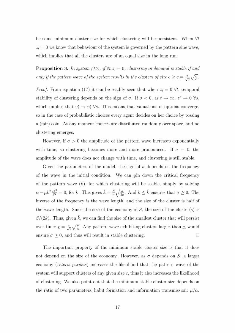
Proposition 3. In system (16), if ∀t zt = 0, clustering in demand is stable if and
only if the pattern wave of the system results in the clusters of size c ≥ c = π√2
√µα
.
Proof. From equation (17) it can be readily seen that when zt = 0 ∀t, temporal
stability of clustering depends on the sign of σ. If σ < 0, as t → ∞, zs → 0 ∀s,
which implies that vs1 → vs2 ∀s. This means that valuations of options converge,
so in the case of probabilistic choices every agent decides on her choice by tossing
a (fair) coin. At any moment choices are distributed randomly over space, and no
clustering emerges.
However, if σ > 0 the amplitude of the pattern wave increases exponentially
with time, so clustering becomes more and more pronounced. If σ = 0, the
amplitude of the wave does not change with time, and clustering is still stable.
Given the parameters of the model, the sign of σ depends on the frequency
of the wave in the initial condition. We can pin down the critical frequency
of the pattern wave (k), for which clustering will be stable, simply by solving
α−µk2 2π2
S2 = 0, for k. This gives k = Sπ
√α2µ
. And k ≤ k ensures that σ ≥ 0. The
inverse of the frequency is the wave length, and the size of the cluster is half of
the wave length. Since the size of the economy is S, the size of the cluster(s) is
S/(2k). Thus, given k, we can find the size of the smallest cluster that will persist
over time: c = π√2
√µα
. Any pattern wave exhibiting clusters larger than c, would
ensure σ ≥ 0, and thus will result in stable clustering.
The important property of the minimum stable cluster size is that it does
not depend on the size of the economy. However, as σ depends on S, a larger
economy (ceteris paribus) increases the likelihood that the pattern wave of the
system will support clusters of any given size c, thus it also increases the likelihood
of clustering. We also point out that the minimum stable cluster size depends on
the ratio of two parameters, habit formation and information transmission: µ/α.
17
There are three distinct behavioural clustering patterns identified in the proof
of proposition 3. These are implied by following three scenarios: σ = 0 (this is
the same as c = c), σ > 0 (c > c) and σ < 0 (c < c).
σ = 0: In this situation the valuation distribution converges to a static sinusoid.
Consequently, the long run valuations are constant. This implies that vsi − vsj is
bounded ∀s. Therefore, the in case of σ = 0 the long run presents only proba-
bilistic clustering in behaviour.
σ > 0: In this case valuation distribution is governed by the sinusoid with ever
increasing amplitude. Therefore, the behaviour in social space is organized as
alternating neighbourhoods of agents with vsi − vsj → ∞ and vsi − vsj → −∞. In
this case polarization among clusters reaches extreme values and the organization
converges to absolute clustering in behaviour.
σ < 0: This is the case when there is no clustering in behaviour, no particular
pattern of organization. Here valuations for the options converge to each other
for every agent. Therefore, every decision maker’s probability of choosing one of
them converges to 0.5. In this case information coming through word-of-mouth is
so strong9 about each of the options, that it confuses the agent, who ultimately
decides to randomly choose between the options.
This result is somewhat similar to the result of “confounded learning” by Smith
and Sorensen (2000). In a sequential choice model with interactions they find a
scenario where the learning process consistently maintains the balance between
the options in the sense that information gathered from other decision-makers
carries no value for the decision process of an agent.
The analysis so far has assumed that each agent has two neighbours (H = 1
on either side). It is interesting how results of the model change if we consider
larger neighbourhoods.
9From equation 18 one can easily see that negative σ is a result of higher rate of communi-cation µ.
18
Proposition 4. In the case of arbitrary an neighbourhood size 2H, where agents
interact with H nearest neighbours on either side, the minimum sustainable cluster
size is
cH =π
2√
3
√2H2 + 3H + 1
õ
α.
The proof of this proposition can be found in appendix C.
Proposition 4 implies that as neighbourhoods grow in size so does the mini-
mum sustainable cluster. The intuition is that a larger neighbourhood facilitates
the information diffusion process: each agent receives information from relatively
distant agents. This works to homogenize the information structure across the
population, and so works against small clusters.
There are a few relevant findings in literature that we can draw parallels with.
For example, Ellison and Fudenberg (1995) find that less communication increases
the likelihood of conformism. In our case we can decompose the “amount” of
communication into intensity of communication (controlled by µ) and the scope of
communication (controlled by H). In our model the outcome of global conformism
does not depend on any model parameters (proposition 1). However, any type of
clustering is conformism and if clustering is local, so is conformism. In our model,
once global conformism is ruled out, the likelihood of local conformism is inversely
related with both µ and H (see equation (25) in the proof of proposition 4).
In Ellison and Fudenberg (1995) slow information exchange ensures multiplicity
of trials before the equilibrium is reached and thus increases the likelihood of
the society learning about the true best option. In our model slow information
exchange gives the chance for groups of agents to “develop the taste” for one
particular option.
A related finding has been reported by Bala and Goyal (2001). They concen-
trate directly on local conformism as the long run outcome. They characterize
the social network by the degree of integration of decision-makers and find that
lower degrees of integration increase the likelyhood of clustering. In our model H
can also be viewed as the degree of integration: higher H means that every agent
interacts with a larger number of other agents. This directly implies a higher level
19
of integration. In this way our results are in line with the findings of Bala and
Goyal (2001): a lower level of integration increases the likelihood that the ampli-
tude growth rate of the dominant sinusoid is positive. Positive σ is a sufficient
condition for local conformism.
On a more general level, the existing literature has examined the effect of the
scope of interaction. In general, the contrast is made between local and global
interactions. Local interactions imply a limited (and usually fixed) subset of other
agents that any given agent interacts with, while global interactions assume that
an information stream from every agent can directly reach any other agent in the
economy. Contrasting these two interaction schemes, researchers find that global
interactions usually result in more ordered systems, while local interaction usually
produces richer and more complex dynamics (e.g. Glaeser and Scheinkman; 2000;
Gonzalez-Avella et al., 2006). This issue can be addressed in our model by looking
at its behaviour as neighbourhoods become very large (H → S/2). According to
proposition 4, increasing the neighbourhood size (H) puts an upward pressure on
the minimum stable cluster size c and for a larger region of parameter space pushes
it above the threshold (c > S/2) beyond which clustering is unstable in the long
run (in the case when the differences between average valuations are zero).10 Thus,
in line with previous research, our model demonstrates that local interactions
result in richer and more complex dynamics than do global interactions.
Based on proposition 4, we can analyze how minimum sustainable cluster size
changes with enlargement of the interaction neighbourhood. It is obvious from
proposition 4 that cH+1 − cH is increasing with H. Moreover, it turns out that
limH→∞
(cH+1 − cH
)=
π√6
õ
α. (19)
Equation 19 implies that for any value of µ/α, minimum sustainable cluster size
increases linearly with the size of the neighbourhood, as long as H is sufficiently
large.
10For example, in the small economy that we have simulated (S = 100), H = 49 implies thatthe speed of habituation, α, must be roughly 80 times as high as the influence of neighbours, µ,in order the system to be stable for the largest possible cluster (c = S/2)
20
4 The multi-option environment
As asserted in the introduction, one of the advantages of the present approach is
that it is straightforward to extend the analysis to a multi-option environment.
In fact the core of the model has been written in this environment and two-option
setup has been chosen only for the demonstration of the major findings in the
previous section.
Proposition 3 describes the relationship between the parameters of the model
and the average cluster size in the long-run, in the two-option case. In this section
we analyze the same relationship for the multi-option environment.
Consider the setup where decision-makers have to choose between N options.
Assume again that agents interact with only two of their neighbours (H = 1). In
this case the dynamics of the model are represented by N equations of the form
of Equation (9). We can choose one of the options as a numeraire (say option
N) and subtract the value of its valuation from every other option for each agent
zn = vn − vN , ∀i 6= N . After rewriting the system in continuous time and space
and applying a Taylor approximation to appropriate terms, the N -option system
will be described by N − 1 equations of the type
∂zn∂t
= αzn + µ∂2zn∂s2
. (20)
The consequence of the separability of inertia is that the dynamics of zn do not
depend on the dynamics of zi, i 6= n.
Every equation in the system (20) has the same form as equation (16). There-
fore, similar to the two-option environment, in this case we again have two differ-
ent outcomes: one in which there is global conformism; the other in which several
choices co-exist in the long run. Which of these scenarios obtains depends on
initial conditions.
As lemma 1 applies to all N −1 equations for identifying the pattern of choice
organization we have to compare the growth patterns of average valuation differ-
ences. As α has the same value across all N − 1 equations, the growth rate of
21
average valuation differences across every option is the same (according to lemma
1, this rate is equal to α). What becomes important is the initial value of the
average valuation for each of the option. It can be shown that the difference be-
tween two variables that grow at an equal exponential rate goes to plus or minus
infinity depending on the sign of the initial value difference. Therefore, we can
formulate the following remark.
Remark 1. In a multi-option environment an option with the highest initial av-
erage valuation will be the only choice for every agent in the long run. Therefore,
there will be absolute clustering and global conformism.
If two or more options have the same, highest initial average valuation, these
will be the only surviving options in the long run. Therefore, for the analysis of
long-run behaviour we can safely drop all inferior practices and concentrate on
those surviving in the long run. In this case the system can be reformulated,
reindexed as the system with several options with equal average initial valuations.
In what follows we restrict attention to this case. For notational simplicity assume
that there are N options with equal initial average valuations.
As it can be readily seen from equation (20) each of the N − 1 equations has
the same form, and the same parameter values, as the unique equation (16) in the
two-option case. Therefore, the following remark is true:
Remark 2. In a multi-option environment, minimum cluster size implied by the
dominant sinusoid of each N − 1 valuation difference distribution is unchanged
from the two-option case, and is equal to cN = c = π√2
√µα
.
Although the solution to the system is very similar to two-option case, its
implications for the organization of behaviour is considerably harder to analyze.
The reason is multiplicity of dominant sinusoids that are present in the system.
However, one important finding that we can directly point out is that for any
option, valuations cluster. That is, the valuation for every option is distributed in
a form of sinusoid in a social space, implying that for any option, nearby agents
have similar valuations. Therefore, the multi-option system should also result in
22
clustering in behaviour (probabilistic or absolute). The only exception to this
will be the case when amplitude growth rates of all N − 1 dominant sinusoids
are negative. In this case each option will have equal chance of being chosen by
any agent in the long run. Furthermore, the probability of clustering increases
with the number of options, as the likelihood of at least one sinusoid having
σ ≥ 0 increases. In other words, increases in the number of options decreases the
likelihood of a coincidence where all σs are negative.
In order to predict clustering patterns we have to compare the amplitude
growth rates of dominant sinusoids. Recall that by equation (18) σ = α−2µπ2
S2k2,
where k ∈ Z+ is the frequency of the sinusoid. As lower k implies higher σ,
as long as initial conditions permit, the fastest growing sinusoid will be the one
corresponding to k = 1. The role of initial conditions requires additional clarifi-
cation. Recall the outline of the proof of lemma 2. If we have S decision-makers,
using a Fourier transform, the initial distribution of choice valuations over social
space can be represented as the sum of waves with k = 1, 2, . . . , S/2, each with
corresponding initial amplitude and its growth rate. As ∂σ/∂k < 0 we know that
out of all the Fourier components the one most likely to become the dominant
wave has the longest wavelength (k = 1). The only case when k = 1 will not
emerge as the dominant sinusoid is if its initial amplitude is equal to zero. In this
case the amplitude will not change over time. The next most probable nominee
for the domination will then be the wave corresponding to k = 2 and so on. This
is true for the valuation distribution of every option.
In the multi-option case what becomes important is not only the dominant
sinusoid for each valuation distribution, but also the competition among the dom-
inant waves across all the options. We know that most of the dominant sinusoids
have the same amplitude growth rate σ = α − 2µπ2
S2 . The rest of the sinusoids
have lower amplitude growth rates. Thus, what becomes important for identifying
the winner, the champion wave, is the initial amplitude. Because the difference
between the amplitudes of two sinusoids with the same (positive) growth rates
and different initial values goes to infinity in the long-run, we can formulate the
23
following remark.
Remark 3. Consider an economy with equal initial average valuations for all
N options. If in this economy there is at least one option characterized by the
dominant sinusoid with a positive growth rate, in the long run there will be an
option that will be consistently chosen by (exactly) half of the population. The
number of clusters where this half of the population will be distributed depends on
the frequency of the champion wave.
Consider a space in which the agents are located along the abscissa and the
ordinate scales the valuation of the different options. The solution to equation
(16) generates a family of sine waves, cycling around the abscissa, each wave
representing the value of each option.11 Amplitudes of the waves are growing, so
over time, one wave (that with the highest growth rate, σ) comes to dominate all
others, and the difference between its amplitude and all others goes to (plus and
minus) infinity. Thus over half the space, it dominates all other options and all
agents (probabilistically) choose that dominant option. But over half the space it
is the least favoured option, and this part of the space is divided among the other
options. We might reasonably expect that as the number of options increases the
probability of finding one large cluster covering half the social space increases.
This simply because the more options the more likely the dominat wave will have
a wave frequency k = 1.
Thus, we have established that half of the social space will be organized in
a few clusters all of which choose the same option. In order to understand how
the other half will be organized note again that we are dealing with sinusoids.
The remaining half of the social space will be shared among the options other
than the champion. In determining how this space is distributed not only the
initial amplitude and amplitude growth rate, but also the location of the sinusoid
becomes important.
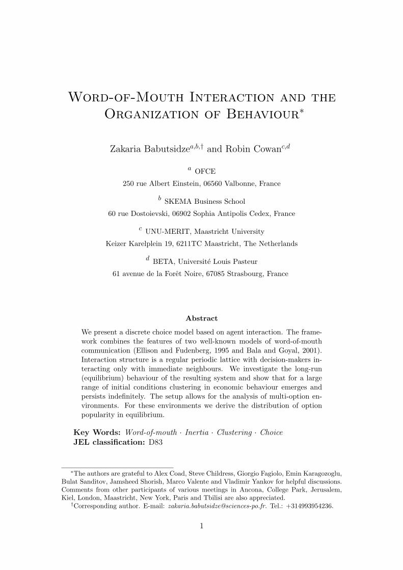
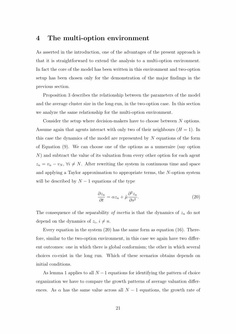
To see why, consider the example shown in Figure 1. There are five options,
and we show their valuations over the social space. One option is a numeraire
11More precisely, one wave for each difference in valuation between an option and a numeraireoption.
24
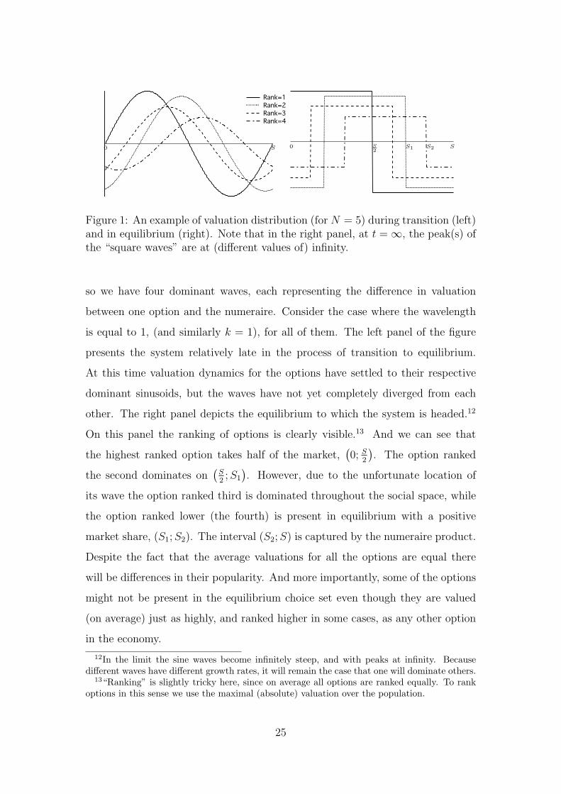
Figure 1: An example of valuation distribution (for N = 5) during transition (left)and in equilibrium (right). Note that in the right panel, at t =∞, the peak(s) ofthe “square waves” are at (different values of) infinity.
S S0 0 S2
S1 S2
so we have four dominant waves, each representing the difference in valuation
between one option and the numeraire. Consider the case where the wavelength
is equal to 1, (and similarly k = 1), for all of them. The left panel of the figure
presents the system relatively late in the process of transition to equilibrium.
At this time valuation dynamics for the options have settled to their respective
dominant sinusoids, but the waves have not yet completely diverged from each
other. The right panel depicts the equilibrium to which the system is headed.12
On this panel the ranking of options is clearly visible.13 And we can see that
the highest ranked option takes half of the market,(0; S
2
). The option ranked
the second dominates on(S2;S1
). However, due to the unfortunate location of
its wave the option ranked third is dominated throughout the social space, while
the option ranked lower (the fourth) is present in equilibrium with a positive
market share, (S1;S2). The interval (S2;S) is captured by the numeraire product.
Despite the fact that the average valuations for all the options are equal there
will be differences in their popularity. And more importantly, some of the options
might not be present in the equilibrium choice set even though they are valued
(on average) just as highly, and ranked higher in some cases, as any other option
in the economy.
12In the limit the sine waves become infinitely steep, and with peaks at infinity. Becausedifferent waves have different growth rates, it will remain the case that one will dominate others.
13“Ranking” is slightly tricky here, since on average all options are ranked equally. To rankoptions in this sense we use the maximal (absolute) valuation over the population.
25
0.5
0.4
0.3
0.2
0.1
0.0
Fn
87654321Rn
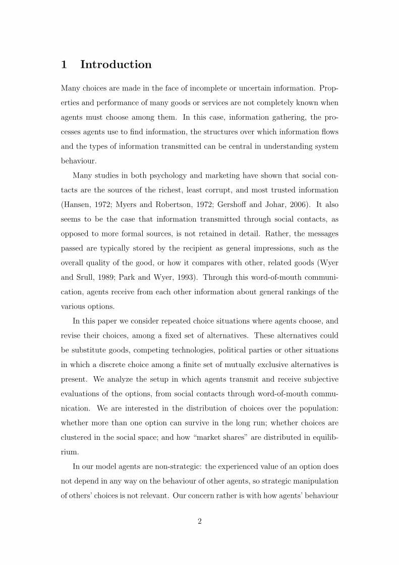
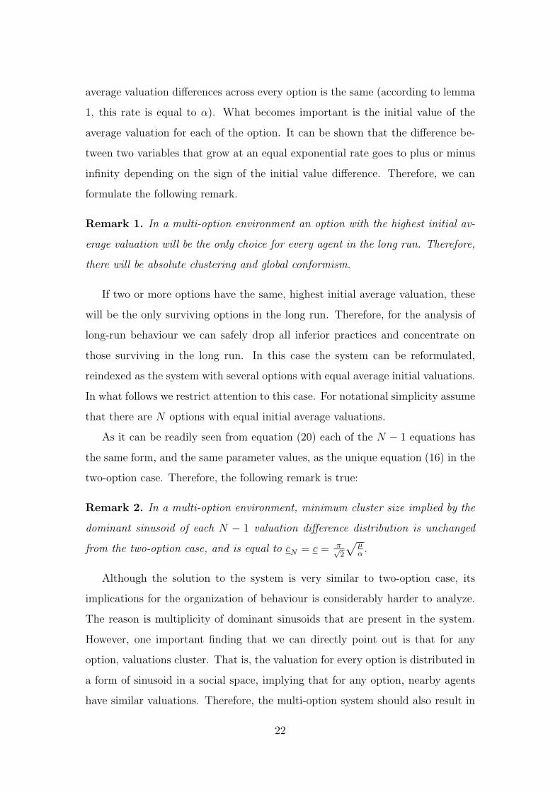
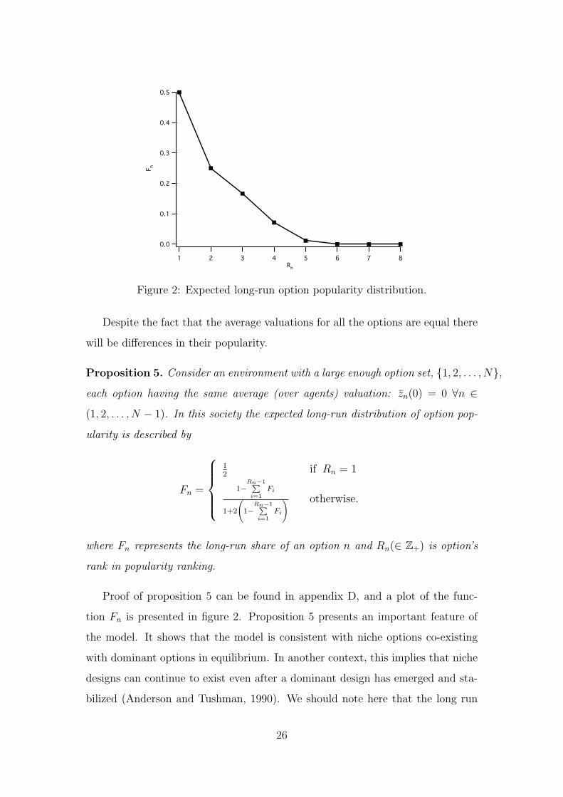
Figure 2: Expected long-run option popularity distribution.
Despite the fact that the average valuations for all the options are equal there
will be differences in their popularity.
Proposition 5. Consider an environment with a large enough option set, {1, 2, . . . , N},
each option having the same average (over agents) valuation: zn(0) = 0 ∀n ∈
(1, 2, . . . , N − 1). In this society the expected long-run distribution of option pop-
ularity is described by
Fn =
12
if Rn = 1
1−Rn−1P
i=1Fi
1+2
1−
Rn−1Pi=1
Fi
! otherwise.
where Fn represents the long-run share of an option n and Rn(∈ Z+) is option’s
rank in popularity ranking.
Proof of proposition 5 can be found in appendix D, and a plot of the func-
tion Fn is presented in figure 2. Proposition 5 presents an important feature of
the model. It shows that the model is consistent with niche options co-existing
with dominant options in equilibrium. In another context, this implies that niche
designs can continue to exist even after a dominant design has emerged and sta-
bilized (Anderson and Tushman, 1990). We should note here that the long run
26
distribution of option adoption (or market share) is independent of the parameters
of the model (given that we satisfy the constraints to preserve variety).
In the economy described in proposition 5 the distribution of choices is the
same as the cluster size distribution. This is due to the fact that the large number
of options ensures that all options chosen in equilibrium have dominant sinusoids
with frequency equal to one.14
To understand why this is the case, consider a single option. Its valuation
across the population at any point in time can be represented by a sum of sinusoids
of various frequencies and amplitudes. Over time the amplitudes of these waves
change, as the option becomes more or less valued by different agents, relative
to the other options. Equation (18) implies that the sinusoid with the lowest
frequency has the highest amplitude growth rate. Therefore, if the wave with the
lowest frequency (k = 1) has non-zero initial amplitude it will become the pattern
wave of the option and it will describe the agent valuations for the option in
equilibrium. Due to the fact that the model has random initial conditions there is
a (fixed) nonzero probability that any option will be characterized by the pattern
wave with the lowest possible frequency.
Initial conditions can be thought of as a random matrix, Mi,j each cell of
which represents the valuation of agent i for option j. It is natural to read this
matrix horizontally, thinking of each agent having a valuation vector over options.
However, reading vertically, we see that this is equivalent to each option having a
“vector” of valuations over agents. In continuous space, this “vector” is a function
that can be described by a sum of sinusoids. There exist (a non-zero measure of)
such functions in which the sinusoid description includes a wave of frequency one
with non-zero amplitude. If the number of options is large enough, then, there
will be a strictly positive number with a non-zero amplitude low frequency (k = 1)
sinusoid in the sum. Those waves all grow at the same speed, and in the limit will
solely describe corresponding options.15
14This is similar to the case presented in figure 1.15This argument suggests that one might need many options to guarantee this condition. In
fact, however, the probability that a function decomposed into sinusoids has a low frequencywave of zero amplitude is vanishingly small. Thus a small number of options will typically be
27
The valuation wave for any option has a part of the population where it is
negative, relative to the numeraire. But if there are many low frequency (k = 1)
waves, passing through zero at different agents, for any agent there will be some
low frequency wave that takes on a positive value at her location. This wave (or
one of these waves), because it grows fastest, will determine her preference in the
long run. This means that by assuming there are many options, the equilibrium
pattern will be described by some number of waves with the same frequency,
k = 1.
Remark 4. Some options might never be chosen in the long-run despite the fact
that all the options are equally valued by the society.
This stems from the proof of proposition 5 and is true even if the economy
consists of infinitely many practices in equilibrium and infinite number of agents.16
The number of clusters will increase with the size of the economy. And in reverse,
as the number of options surviving increases, the economy must increase in size.
For example, if sustaining six practices in the long run demands an economy of
1/F6 = 3614 decision makers, sustaining seven practices requires 1/F7 > 6.5×10⁶
agents, and sustaining eight demands 1/F8 > 2.1×10¹³ and so on. So we can say,
for example, that no mater how large is the initial option set, in an economy with
less than 3614 agents, at most only five options can survive in the long run.
5 Emergence of Novelty
In the dynamics we model, word-of-mouth interaction is a force moving the system
towards the homogenization of valuation profiles across neighbours. As expressed
in equation (1), agents partially conform to each others views as a result of in-
teraction. On the other hand, inertia at the agent level reinforces every agent’s
current choice profile. Therefore, agents in the interior of a cluster (ones which
are surrounded by like-minded agents) get doubly encouraged to stick to their
enough to produce this condition.16If the number of decision-makers is finite, due to the integer problem (cluster size cannot
be less then one agent), there will always be only a finite number of clusters in the economy.
28

current choices. As a larger cluster implies a higher number of agents located in
the interior, we can expect larger clusters to have higher growth potential.
But we can also expect that initial development of the industry will be noisy.
It will involve shrinking and the ultimate disappearance of certain clusters at the
expense of the growth of others. This suggests that these growing clusters will be
the large clusters, and shrinking ones will be the ones that are relatively small.
Although true in a general sense, this statement does not describe the whole story.
It is also the case that new behaviour can emerge in locations it has not been seen,
diffuse and even survive in the long run.
Options can emerge (and become popular) in locations with no prior history
of similar behaviour. Consider the following simple example. Agent s − 1 ranks
option 1 first and option 3 last; agent s+ 1 ranks option 3 first and option 1 last.
Both agents, though, rank option 2 second. It is clear that agent s, based on
the information communicated to her, could easily come to rank option 2 before
either 1 or 3. If the relatively high rankings of option 2 by s − 1 and s + 1 have
emerged (due to information received by their neighbours) at roughly the same
time, agent s can then switch to option 2, regardless of what he was doing in the
past. Maintaining the practice for longer period and passing negative information
about option 1 to agent s− 1 and about option 3 to agent s+ 1, it is also possible
that agent s will induce both agents to abandon their choices and switch to option
2.17
To demonstrate that this kind of behaviour is possible (and in fact not improb-
able in the early stages of industry development) we perform a small numerical
exercise. Set the number of options to N = 10; and the population size to S = 100.
The population is located on a one-dimensional periodic lattice, so the neighbours
of agent 1 are agents 2 and 100. Set the parameters α = 0.001 and µ = 0.01.
Finally, each agent has one neighbour on either side, H = 1. Initially, agents are
randomly assigned a valuation vector. These valuations are updated each period
17Even though emergence of novelty can also be observed in a similar model without rumors(agents transmitting information only about the products that they have consumed during theperiod), the richer communication channel including rumors substantially expands relaxes theconditions under which emergent novelty can be observed.
29
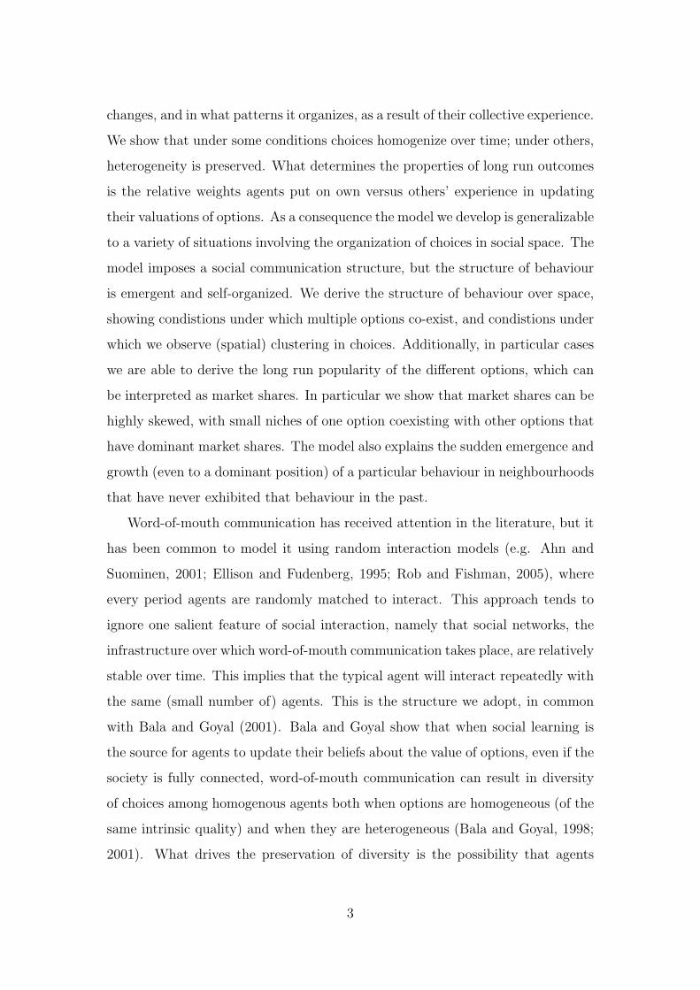
1 25 50 75 100
Agent
0
500
1000
1500
2000
Time
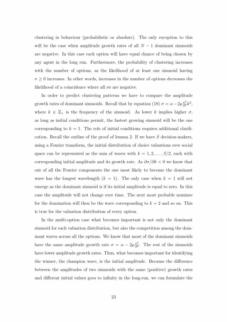
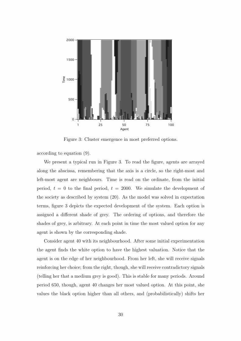
Figure 3: Cluster emergence in most preferred options.
according to equation (9).
We present a typical run in Figure 3. To read the figure, agents are arrayed
along the abscissa, remembering that the axis is a circle, so the right-most and
left-most agent are neighbours. Time is read on the ordinate, from the initial
period, t = 0 to the final period, t = 2000. We simulate the development of
the society as described by system (20). As the model was solved in expectation
terms, figure 3 depicts the expected development of the system. Each option is
assigned a different shade of grey. The ordering of options, and therefore the
shades of grey, is arbitrary. At each point in time the most valued option for any
agent is shown by the corresponding shade.
Consider agent 40 with its neighbourhood. After some initial experimentation
the agent finds the white option to have the highest valuation. Notice that the
agent is on the edge of her neighbourhood. From her left, she will receive signals
reinforcing her choice; from the right, though, she will receive contradictory signals
(telling her that a medium grey is good). This is stable for many periods. Around
period 650, though, agent 40 changes her most valued option. At this point, she
values the black option higher than all others, and (probabilistically) shifts her
30
behaviour accordingly. But interestingly, black was not valued highly (and thus
only consumed infrequently, if at all) in her neighbourhood prior to her switch.
This switch introduces a novel option to the neighbourhood. With time this new
practice becomes popular in the neighbourhood, survives and expands, at least
until period 2000. A similar pattern appears at later stage of development in the
run, when agent 96 decides to experiment at t ≈ 1400. Again, the very-dark-grey
option emerges as most valued, even though it was not present as the favorite
anywhere in the neighbourhood. It too survives and expands in popularity.
We see that behavioural clusters can emerge, apparently ex nihilo, in social
space. Rumors from different sources can aggregate to a signal powerful enough
to induce agents with narrow margins at the top of their rankings to switch to
an unexplored alternative. Thus, our model is consistent not only with shrinking
and disapearance of smaller clusters, but also with the emergence and growth of
new ones.18
6 Conclusion
In this paper we have argued that interaction with peers over social networks can
have important effects on the organization of behaviour. This external force, to-
gether with internal forces such as inertia, generate rich choice dynamics among
mutually exclusive options. Information diffusion through fixed social networks
naturally generates clustering in behaviour: some neighbourhoods collectively pre-
fer one option over another, while other neighbourhoods do the reverse. But de-
pending on the characteristics of the society, this pattern can be either fragile or
stable. In essence, several parallel informational cascades can result in persistent
lateral distributions in social space, where clearly identified neighbourhoods have
18Figure 3 presents the evolution of the most preferred option, driven by system (20). Thisis not necessarily the evolution of choices, as choices are only probabilistically determined byvaluations. Because actual behaviour is “noisy” in this sense, it is more difficult to observe theemergence of pure novelty in behaviour, unless the function mapping valuation to behaviourhas a very steep gradient near 1. However, even with less severe gradients, it is not uncommonto observe behaviour that was rare (and sometimes completely absent) in a neighbourhoodemerging and growing to become common in that neighbourhood, and beyond.
31
higher concentrations of one particular type of information (information about one
option), or to put it differently, where the peaks of different positive informational
cascades (Hirshleifer, 1993) are located in different places in social space.
The model presented in this paper, in which information is transmitted by
word-of-mouth, includes the ability of agents to transmit “rumours” through so-
cial interaction. The framework we have developed is extended beyond the two-
option case that is typical in the literature. We show that system behaviour in
the multi-option case is similar to the two option case, but including more than
two options in the analysis permits us to extend the framework and derive more
reasonable results on the distribution of “market shares” of the options. The
extension to multiple options means that the model can be applied not only to
binary choice situations, such as bribery or criminal activity, but also to voting
in multi-party systems or product choice in multi-product environments. The
model reproduces many analytical and empirical findings, such as clustering in
social space, emergence of conformism, existence and stability of market niches.
However, by including the ability of agents to transmit rumours, we can avoid
the “must see to adopt” assumption common in the literature, and so are able to
explain not only the fact that clusters increase, decrease, or stabilize, but also pro-
vide a natural explanation of the emergence of novelty. In this model behaviour
previously unseen in a neighbourhood can suddenly appear, grow and even come
to dominate.
References
Abel, A. B. (1990): “Asset Prices under Habit Formation and Catching up with
the Joneses,” The American Economic Review, 80(2), 38–42.
Ahn, I., and M. Suominen (2001): “Word-of-Mouth Communication and Com-
munity Enforcement,” International Economic Review, 42(2), 399–415.
Anderson, P., and M. L. Tushman (1990): “Technological Discontinuities and
32
Dominant Designs: A Cyclical Model of Technological Change,” Administrative
Science Quarterly, 35(4), pp. 604–633.
Anderson, S. P., A. de Palma, and J.-F. Thisse (1992): Discrete Choice
Theory of Product Differentiation. MIT press, Cambridge.
Arnade, C., M. Gopinath, and D. Pick (2008): “Brand Inertia in U.S.
Household Cheese Consumption,” American Journal of Agricultural Economics,
90(3), 813–826.
Bala, V., and S. Goyal (2001): “Conformism and diversity under social learn-
ing,” Economic Theory, 17(1), 101–120.
Banerjee, A. V. (1992): “A Simple Model of Herd Behavior,” The Quarterly
Journal of Economics, 107(3), 797–817.
(1993): “The Economics of Rumours,” The Review of Economic Studies,
60(2), 309–327.
Banerjee, A. V., and D. Fudenberg (2004): “Word-of-mouth learning,”
Games and Economic Behavior, 46(1), 1–22.
Bikhchandani, S., D. Hirshleifer, and I. Welch (1992): “A Theory of
Fads, Fashion, Custom, and Cultural Change as Informational Cascades,” The
Journal of Political Economy, 100(5), 992–1026.
Bjonerstedt, J., and J. Weibull (1995): “Nash Equilibrium and Evolution
by Imitation,” in The Rational Foundations of Economic Behavior, ed. by K. J.
Arrow, E. Colombatto, M. Perlman, and C. Schmidt. McMillan, New York.
Chintagunta, P., E. Kyriazidou, and J. Perktold (2001): “Panel data
analysis of household brand choices,” Journal of Econometrics, 103(1-2), 111 –
153.
Chintagunta, P. K. (1998): “Inertia and Variety Seeking in a Model of Brand-
Purchase Timing,” Marketing Science, 17(3), 253–270.
33
Constantinides, G. M. (1990): “Habit Formation: A Resolution of the Equity
Premium Puzzle,” The Journal of Political Economy, 98(3), 519–543.
Ellis, R. (1985): Entropy, Large Deviations, and Statistical Mechanics. Springer-
Verlag, New York.
Ellison, G., and D. Fudenberg (1993): “Rules of Thumb for Social Learn-
ing,” The Journal of Political Economy, 101(4), 612–643.
(1995): “Word-of-Mouth Communication and Social Learning,” The
Quarterly Journal of Economics, 110(1), 93–125.
Fujita, M., P. Krugman, and A. Venables (1999): The Spatial Economy.
MIT press, Cambridge.
Gershoff, A. D., and G. V. Johar (2006): “Do You Know Me? Consumer
Calibration of Friends’ Knowledge,” Journal of Consumer Research, 32, 496–
503.
Glaeser, E. L., and J. A. Scheinkman (2000): “Non-Market Interactions,”
working paper 8053, NBER.
Gonzalez-Avella, J. C., V. M. Eguiluz, M. G. Consenza, K. Klemm,
J. L. Herrera, and M. San-Miguel (2006): “Local versus Global Inter-
action in Nonequilibrium Transitions: A Model of Social Dynamics,” Physical
Review E, 73, 1–7.
Hansen, F. (1972): Consumer Choice Behavior: A Cognitive Theory. The Free
Press, New York.
Hirshleifer, D. (1993): “The Blind Leading the Blind: Social Influence, Fads
and Information Cascades,” working paper 24’93, Anderson Graduate School
of Management.
Ioannides, Y. (2006): “Topologies of social interactions,” Economic Theory,
28(3), 559–584.
34
Myers, J. H., and T. S. Robertson (1972): “Dimensions of Opinion Leader-
ship,” Journal of Marketing Research, 9(1), 41–46.
Park, J.-W., and R. S. Wyer (1993): “The Cognitive Organization of Product
Information: Effects of Attribute Category Set Size on Information Recall,”
Journal of Consumer Psychology, 2, 329–357.
Pope, R., R. Green, and J. Eales (1980): “Testing for Homogeneity and
Habit Formation in a Flexible Demand Specification of U.S. Meat Consump-
tion,” American Journal of Agricultural Economics, 62(4), 778–784.
Quah, D. (2000): “Internet cluster emergence,” European Economic Review,
44(4-6), 1032 – 1044.
(2002): “Spatial Agglomeration Dynamics,” The American Economic
Review, 92(2), pp. 247–252.
Ravn, M., S. Schmitt-Grohe, and M. Uribe (2006): “Deep Habits,” The
Review of Economic Studies, 73(1), 195–218.
Rob, R., and A. Fishman (2005): “Is Bigger Better? Customer Base Expan-
sion through Word-of-Mouth Reputation,” The Journal of Political Economy,
113(5), 1146–1162.
Schlag, K. (1998): “Why immitate and if so, how? A boundedly rational
approach to multiarmed bandits,” The Journal of Economic Theory, (130–156).
Smith, L., and P. Sorensen (2000): “Pathological Outcomes of Observational
Learning,” Econometrica, 68(2), 371–398.
Turing, A. M. (1952): “The Chemical Basis of Morphogenesis,” Philosophical
Transactions of the Royal Society of London, Series B, Biological Science, 237,
37–72.
Witt, U. (2001): “Learning to Consume - A Theory of Wants and the Growth
of Demand,” Journal of Evolutionary Economics, 11, 23–36.
35

Wyer, R. S., and T. K. Srull (1989): Memory and Cognition in its Social
Context. Lawrence Erlbaum Associates: New Jersey.
36
Appendix
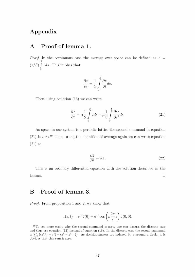
A Proof of lemma 1.
Proof. In the continuous case the average over space can be defined as z =
(1/S)S∫0
zds. This implies that
∂z
∂t=
1
S
S∫0
∂z
∂tds.
Then, using equation (16) we can write
∂z
∂t= α
1
S
S∫0
zds+ µ1
S
S∫0
∂2z
∂s2ds. (21)
As space in our system is a periodic lattice the second summand in equation
(21) is zero.19 Then, using the definition of average again we can write equation
(21) as
∂z
∂t= αz. (22)
This is an ordinary differential equation with the solution described in the
lemma.
B Proof of lemma 3.
Proof. From proposition 1 and 2, we know that
z(s; t) = eαtz(0) + eσt cos
(k
2π
ls
)z(0; 0).
19To see more easily why the second summand is zero, one can discuss the discrete caseand thus use equation (12) instead of equation (16). In the discrete case the second summandis∑s
((zs+1 − zs)− (zs − zs−1)
). As decision-makers are indexed by s around a circle, it is
obvious that this sum is zero.
37
Substituting this into equation (16) and noticing that
∂2 cos(βx)/∂x2 = −β2 cos(βx),
allows us to solve for σ.
C Proof of proposition 4.
Proof. Consider the case of arbitrary neighbourhood size of 2H. In this case after
assuming that the distance between two neighbouring agents is δ and considering
the two-option case, continuous version of equation (9) can be rewritten as
∂z(s)
∂t= αz(s) +
µ
2H
H∫−H
z(s+ δh)dh− 2Hz(s)
. (23)
Using second order taylor approximation we can rewrite the part of (23) under
the integral as
H∫−H
z(s)dh+
H∫−H
δh∂z(s)
∂sdh+
H∫−H
δ2h2
2
∂2z(s)
∂s2dh.
Which, after integration of first two summands, is equal to
2Hz(s) + 0 +δ2
2
∂2z(s)
∂s2
H∫−H
h2dh.
To obtain more accurate values for smaller neighbourhood size, we go back to
discrete space and replace the integral in expression above with the sum of squares
of integer values.
Substituting this result back to (23) yields
∂z(s)
∂t= αz(s) +
µδ2
4H
H∑h=−H
h2∂2z(s)
∂s2.
Thus, it follows that the only modification that this generalization brings to
38
the system can be captured by the definition of µ in the text being changed to
µ =µδ2
4H
H∑h=−H
h2. (24)
Going back to agent addresses (δ = 1), using new definition of µ, and the
identityx∑
n=1
n2 = x3
3+ x2
2+ x
6we can rewrite equation (18) as
σH = α− 2µ(kπ
l
)2(H2
3+H
2+
1
6
), (25)
which results in
kH =S
π
√α
(2µ
(H2
3+H
2+
1
6
))−1
, (26)
and further in
cH =π
2√
3
√2H2 + 3H + 1
õ
α. (27)
D Proof of proposition 5.
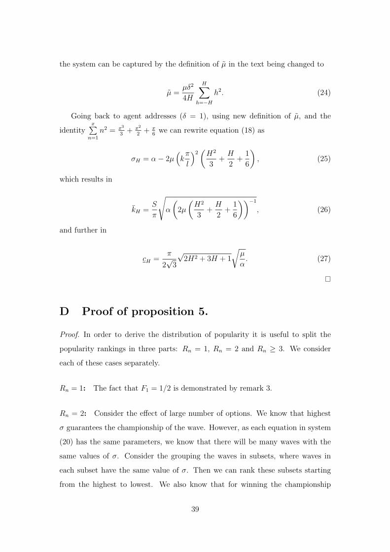
Proof. In order to derive the distribution of popularity it is useful to split the
popularity rankings in three parts: Rn = 1, Rn = 2 and Rn ≥ 3. We consider
each of these cases separately.
Rn = 1: The fact that F1 = 1/2 is demonstrated by remark 3.
Rn = 2: Consider the effect of large number of options. We know that highest
σ guarantees the championship of the wave. However, as each equation in system
(20) has the same parameters, we know that there will be many waves with the
same values of σ. Consider the grouping the waves in subsets, where waves in
each subset have the same value of σ. Then we can rank these subsets starting
from the highest to lowest. We also know that for winning the championship
39
in case of equal σs what matters is the initial amplitude. Then in each subset
we can rank waves in decreasing order of their initial amplitude values. Now we
have a unique ranking of all the waves. We call this a preliminary ranking as
some of the waves might get dropped from the top places due to the subsequent
refinement. We will demonstrate that not every option will appear in the long
run frequency distribution. As higher waves in ranking have higher chances for
ending up in the frequency distribution we assume that the set of options is so large
that all the ultimate practices will be selected from the highest ranked subgroup.
Therefore, we simply disregard lower ranked subgroups. Thus, large number of
options ensures that every option present in the long run frequency distribution
with a non-zero weight has the wave length of k = 1.
We know that the most popular option has half of the market size. As large
number of options ensures that the champion wave has the wave length of k = 1,
and thus the most popular option has one cluster (of size S/2) in the social space.
As our social space is circular we can reindex the agents without loss of generality.
Assume the champion sinusoid starts at agent s = 0. This would mean, that the
cluster of the champion practice comprises the social space between s = 0 and
s = S/2. Now, what becomes important for identifying the size of the second
largest cluster is the offset of the second ranked wave from the champion. Offset
if the difference in social space between the sinusoid under discussion and the
champion sinusoid. As we normalized the champion to start at s = 0, the offset
of any wave will simply be equal to the location s where they start. To identify
which option is going to be the second most popular in the long run we go down
the preliminary ranking. If the second ranked option in the preliminary ranking
has offset exactly equal to zero this means that this sinusoid is positive in space
(0;S/2) and negative in (S/2; 1). But so is the champion wave. And we know that
champion dominates any other wave completely in the space (0;S/2). Therefore,
the wave with offset zero will never show up in the long run frequency distribution
with the positive weight. Thus, we can discard the wave and remove it from the
rankings.
40
Then we go down to the rankings until we find the wave with offset si > 0.
Consider how the share of social space dominated by this option depends on si. If
si < S/2 we know that this wave will be positive on (si;S/2 + si) and negative on
(0; si) ∪ (S/2 + si; 1). However, on(si;S/2) if will be dominated by the champion
wave, therefore this option will only acquire S/2 + si−S/2 = si part of the social
space. In case when si > S/2 the wave is positive on (si; 1)∪ (0;S/2−1+si). But
it is dominated by the champion on fraction (0;S/2− 1 + si), and thus, it obtains
the section 1 − si. It can be easily seen that as si goes from si = 0 to si = S/2,
the part dominated by the second ranked wave also increases linearly from zero
to S/2. As si continues move to the right after passing S/2, the part dominated
by the wave decreases linearly from S/2 to zero (when si = 1).
Now, as initial conditions are random and agents are distributed uniformly
over the social space, the probability of choice of any si is constant. Therefore,
we can calculate that the average market share of the second ranked practice in
the long run F2 = 1/4. In order to build the case for Rn > 2 notice that there are
two actual waves corresponding to the market share of 1/4. These are si = S/4
and and si = 3S/4. It does not matter for the further calculations which of
them we choose to be present while considering Rn > 2 options. Because of the
circularity of social space, there will always be two waves corresponding to each
share distribution. Without loss of generality we always choose to consider that
the wave with the smaller si is at place. Thus, for later options there will always
be some space (0;W > S/2) that we be occupied by stronger waves and the space
(W ; 1) left to be distributed among the weaker waves.
Rn = m > 2: As pointed out in case Rn = 2, by now the social space (0;W ) is
already distributed. Then W =m−1∑j=1
Fj. Denote the size of the remaining social
space w = 1−W . Then, w is the size of the not-yet-distributed portion. In this
case, the we know that the weakest wave already assigned its long-run share is the
wave with the positive part on (S/2−w; 1−w). Therefore, any wave to be placed
next on the social space has to have the offset more than si > S/2 − w. This is
because the waves with less offset will always be dominated by the already the
41

most popular m− 1 waves. Therefore, while going down the preliminary ranking
we through out all the waves with offset less then S/2− w, and concentrate only
on offsets with higher offsets.
Consider how long-run market share depends on si in this case. With si
increasing from S/2 − w till S/2 the share increases linearly from zero to w. In
the section where si ∈ (S/2; 1 − w) the share is constant at w. Once si passes
1− w the share decreases linearly and reaches zero at si = 1. In this case taking
the average long run market size and converting it to shares results in
Fm =w
1 + 2w.
It is easy to check that m = 2 also obeys this formula (although the calculation of
F2 was slightly different, it was in fact the specific case of these calculations).
42