Wolfgang Leininger

#49

Ruhr

Econ

omic

Pape

rs

Ruhr Economic PapersPublished byRuhr-Universität Bochum (RUB), Department of EconomicsUniversitätsstraße 150, 44801 Bochum, GermanyTechnische Universität Dortmund, Department of Economic and Social SciencesVogelpothsweg 87, 44227 Dortmund, GermanyUniversität Duisburg-Essen, Department of EconomicsUniversitätsstraße 12, 45117 Essen, GermanyRheinisch-Westfälisches Institut für Wirtschaftsforschung (RWI Essen)Hohenzollernstrasse 1/3, 45128 Essen, Germany

Editors:Prof. Dr. Thomas K. BauerRUB, Department of EconomicsEmpirical EconomicsPhone: +49 (0) 234/3 22 83 41, e-mail: thomas.bauer@rub.deProf. Dr. Wolfgang LeiningerTechnische Universität Dortmund, Department of Economic and Social SciencesEconomics – MicroeconomicsPhone: +49 (0) 231 /7 55-32 97, email: W.Leininger@wiso.uni-dortmund.deProf. Dr. Volker ClausenUniversity of Duisburg-Essen, Department of EconomicsInternational EconomicsPhone: +49 (0) 201/1 83-36 55, e-mail: vclausen@vwl.uni-due.deProf. Dr. Christoph M. SchmidtRWI EssenPhone: +49 (0) 201/81 49-227, e-mail: schmidt@rwi-essen.de

Editorial Office:Joachim SchmidtRWI Essen, Phone: +49 (0) 201/81 49-292, e-mail: schmidtj@rwi-essen.de

Ruhr Economic Papers #49Responsible Editor: Wolfgang LeiningerAll rights reserved. Bochum, Dortmund, Duisburg, Essen, Germany, 2008ISSN 1864-4872 (online) – ISBN 978-3-86788-052-7

The working papers published in the Series constitute work in progress circulated tostimulate discussion and critical comments. Views expressed represent exclusivelythe authors’ own opinions and do not necessarily reflect those of the editors.

Ruhr Economic Papers#49

Wolfgang Leininger

Bibliografische Information der Deutschen NationalbibliothekDie Deutsche Nationalbibliothek verzeichnet diese Publikation inder Deutschen Nationalbibliografie; detaillierte bibliografische Datensind im Internet über http://dnb.d-nb.de abrufbar.

ISSN 1864-4872 (online)ISBN 978-3-86788-052-7

Wolfgang Leininger*

Evolutionarily Stable Preferences in Contests

AbstractWe define an indirect evolutionary approach formally and apply it to(Tullock)contests. While it is known (Leininger, 2003) that the direct evolu-tionary approach in the form of finite population ESS (Schaffer, 1988) yieldsmore aggressive behavior than in Nash equilibrium, it is now shown that theindirect evolutionary approach yields the same more aggressive behavior, too.This holds for any population size N, if evolution of preferences is determinedby behavior in two-player contests. The evolutionarily stable preferences(ESP) of the indirect approach turn out to be negatively interdependent,thereby “rationalizing” the more aggressive behavior.

JEL Classification: C 79, D 72

July 2008

* University of Dortmund (TU), Department of Economics, D-44221 Dortmund,wolfgang.leininger@udo.edu.

1 Introduction

Contest models based on a family of contest success functions, which was introducedby Tullock (1980), have become a standard workhorse of contest and conflict theory;this is true for both, the growing number of economic and non-economic areas ofapplications of contest theory as well as the theoretical advancement of contesttheory itself (see e.g. the survey volumes edited by Lockard and Tullock (2001) and- most recently - Congleton, Hillman and Konrad (2008)). The present paper henceaddresses a new theoretical question on purpose in the framework of Tullock‘s modelwithout striving for utmost generality of results.

Most of the theoretical body of contest theory, and in particular rent-seeking theory,is based on the solution concept Nash equilibrium. Only recently have evolutionarysolution concepts like the notion of an evolutionarily stable strategy (ESS) success-fully entered the field, in particular in the notion of Schaffer‘s (1988) adaptationof the standard notion of an ESS (Maynard-Smith, 1974) to finite population ofplayers. While the latter amounts to a refinement of Nash equilibrium, the formercan, but need not, be different from Nash equilibrium. Leininger (2003) shows, thatfor a large class of contest success functions, including Tullock contest success func-tions, the two solution concepts must always give different solutions. Hehenkamp,Leininger and Possajennikov (2004) provide a full ESS-analysis of Tullock‘s originalcontest model and relate the results to those of the Nash-based theory. Among themost striking results is the observation, that overdissipation of the rent can be anESS-outcome of the contest. Further analyses of contests, which use Schaffer‘s con-cept are contained in Leininger (2006), Schmidt(2007), and Hehenkamp (2007). Allthese papers refer to evolution of strategies, respectively behavior; i.e. the solutionconcept ESS is applied to the strategy sets of a game with fixed preferences, whichcould be termed the standard (or direct) evolutionary approach. In contrast, Guthand Yaari (1992) have pioneered (and termed) an indirect evolutionary approach, inwhich evolution operates at the level of preferences, while actions are still determinedby Nash equilibrium w.r.t. fixed strategy sets. The quest then is for evolutionarilystable preferences (ESP). Guth and Peleg (2001) have addressed this question w.r.t.Maynard-Smiths‘ notion of ESS by searching for conditions under which standardpayoff (maximization) is evolutionarily stable, while Warneryd (2008) has identifiedevolutionarily stable preferences w.r.t. Schaffer‘s ESS notion in a contest model, inwhich cost parameters evolve evolutionarily.

The present paper goes one step further by investigating the relation between be-havior determined by the direct evolutionary approach at the level of strategies andthe indirect evolutionary approach at the level of preferences. We develop bothapproaches in detail and apply them to simple versions of an indirect evolutionary

4

Tullock contest. As is standard in evolutionary game theory we mainly concentrateon two-player evolutionary games, which, however, are played by populations of ar-bitrary size. For each population size we determine evolutionarily stable preferences(ESP) uniquely and relate Nash equilibrium behavior w.r.t. ESP to behavior whichresults from applying ESS to strategies directly according to the direct evolutionaryapproach. Our main finding is that both approaches determine the same behaviorfor all sizes of the population.

The paper is organized as follows: Section 2 summarizes Nash solution theory (Tul-lock 1980) and ESS solution theory (Hehenkamp et al. 2004) of Tullock contests.Section 3 introduces the indirect evolutionary approach, while section 4 gives anillustrative example of a Tullock contest, in which non-standard preferences yield anevolutionary advantage over standard preferences. Section 5 presents the indirectevolutionary game and its solution concept in detail. Section 6 contains the mainbody of analysis of two-player evolutionary games with variable population size.Section 7 concludes.

2 Nash behavior and evolutionarily stable behav-

ior

Recall that Tullock (1980) proposed a model, in which n rent-seekers compete for arent of size V . If the contestants expend x = (x1, ..., xn), xi ≥ 0, the probability ofsuccess for player i, i = 1, ..., n is given by

pi(x1, ..., xn) =xr

in∑

j=1xr

j

and expected profit for player i is given by

Πi(x1, ..., xn) = pi(x1, ..., xn)V − xi =xr

in∑

j=1xr

j

V − xi.

One can show that for r ≤ n/(n − 1), a unique Nash equilibrium in pure strategiesexists in this game, in which each player maximizes expected payoff by bidding

x∗ = n−1n2 rV .

Aggregate rent-dissipation then amounts to

nx∗ = n−1n

rV .

5

Equilibrium expenditures never exceed V , the value of the rent, but may be strictlyless than V . The ”full rent dissipation”-hypothesis does not hold; yet overdissipationis incompatible with individually rational payoff maximization as it would imply,that at least one contestant has a negative payoff in equilibrium (and would thereforebe better off by non-participation or bidding zero).

Later Hehenkamp, Leininger and Possajennikov (2004) used the concept of an evo-lutionarily stable strategy (ESS) for finite population (Schaffer, 1988) to reanalysethis game.

A strategy is evolutionarily stable, if a whole population using that strategy cannotbe invaded by a sufficiently small group of ”mutants” using another strategy. Simi-larly, a standard of behavior in an economic contest is evolutionarily stable, if - uponbeing adopted by all participants in the contest - no small subgroup of individualsusing a different standard of behavior can invade and ”take over”. Obviously, inthe context of finite populations the smallest meaningful number of mutants is one.The emphasis of the evolutionary approach is not on explaining action (as a resultof particular choice or otherwise), but on the diffusion of forms of behavior in groups(as a result of learning, imitation, reproduction or otherwise).

The definition of invadability is all important:

Definition 1:

i) Let a strategy (standard of behavior) x be adapted by all players i, i = 1, ..., n.A mutant strategy x �= x can invade x, if the payoff for a single player using x(against x of the (n − 1) other players) is strictly higher than the payoff of aplayer using x (against (n− 2) other players using x and the mutant using x).

ii) A strategy xESS is evolutionarily stable, if it cannot be invaded by any otherstrategy.

Roughly speaking, an ESS is such that, if almost all members of a group adoptit, there is no other strategy that could give a higher relative payoff, if used bya group member. The dynamic justification for this notion of equilibrium is, thatmore successful strategies diffuse or ”reproduce” faster than less successful onesand ultimately extinguish the latter. Formally, consider a group of N potentialcontestants, who may recurrently engage in a contest of size n < N ; i.e. only n outof N contestants compete in the contest. The expected payoff of a single mutantamong the N contestants if he is drawn into a contest and plays a strategy x against(n − 1) other players using strategy x is then still given by

Π1(x, x, ..., x) = xr

(n−1)xr+xr V − x;

6

but one of the other (n − 1) players i, i ∈ {2, ..., n}, chosen for the contest expects

Πi = (1 − n−1N−1

)Πi(x, ..., x) + n−1N−1

Πi(x, x, ..., x)

as the probability, that a chosen player i will face the mutant player 1 from theremaining (N − 1) potential players among the further chosen (n − 1) players is(n−1)/(N−1). Note that we have assumed that players are chosen for participationrandomly and with equal probability. Consequently, an ESS strategy xESS must nowsolve the problem (Schaffer, 1988) of relative payoff maximization

maxx

Π1(x, xESS, ..., xESS) − (1 − n−1N−1

)Πi(xESS, ..., xESS)

− n−1N−1

Πi(x, xESS, ..., xESS)

Eliminating the constant term (1− (n− 1)/(N − 1))Πi(xESS, ..., xESS) equivalently

yields

(E) maxx

Π1(x, xESS, ..., xESS) − n−1N−1

Πi(x, xESS, ..., xESS).

We can directly read off from the maximand, that as N → ∞ we approach theNash equilibrium problem and hence the difference in behavior among n contestantsin Nash equilibrium and among n contestants (chosen out of large population ofpotential contestants) in evolutionary equilibrium disappears.

Hehenkamp et al. (2004, Theorem 5) show that for r ≤ n/(n − 1) a unique ESSexists, in which each player maximizes relative payoff by bidding

(DE) xESS = n−1n2

NN−1

rV .

Hence a unique ESS exists under precisely those circumstances, which imply exis-tence of a Nash equilibrium (NE) in pure strategies. Both concepts predict differentbehavior for a population of N = n players! ESS behavior is more aggressive asxESS = r

nV always exceeds x∗ = (n−1)r

n2 V . Moreover, aggregate ESS-behavior doesnot depend on the number of players involved in the contest, only on the value ofthe price V and the contest technology parameter r as n · xESS = r · V . This meansover-/under-dissipation of the rent if r>

<1; in case r = 1 full rent dissipation applies.

3 The indirect evolutionary approach

The indirect evolutionary approach (Guth and Yaari, 1992) assumes that behaviorevolves evolutionarily indirectly; i.e. the evolutionary forces do not work on actions

7

or strategies directly, but on entities or ”stimuli” which in turn determine or at leastinfluence behavior. A quite general and economically highly relevant case occurswhen such genetically determined stimuli shape individual preferences of players.Evolutionary forces then work towards preference evolution rather than behavior(or strategy) evolution directly.

The indirect evolutionary approach assumes a large population of players, who playan evolutionary game as follows: For expositional clarity let us focus on two-playercontests. From the population pairs of players are randomly drawn into playingthe contest, in which they non-cooperatively interact by choosing a strategy each,which determines outcome and payoffs of the game. Moreover, the outcome of thegame also determines evolutionary fitness according to a ”fitness function”, whichneed not be identical to the payoff function of the players. This is the key insightof the indirect approach that success in short terms of payoff need not coincidewith evolutionary success in the long-run. If, however, players differ with respectto evolutionary success, the more successful will spread faster within the populationthan the less successful and hence their ”stimuli” resp. preferences will becomemore frequent in the population. This triggers an evolutionary process in the spaceof preferences, which determines in the long-run a distribution of evolutionarilystable preferences, which then in turn determine a stable distribution of behavior(as the process of preference evolution has come to a halt). It is this behavior, whichresults from indirect evolution, which we want to compare and relate to behaviorresulting from direct evolution of strategies (as determined by ESS according to theDefinition 1).

More precisely, we shall assume that any two players with whatever preferences (tobe specified later) play according to Nash equilibrium when drawn into a contest.I.e. they behave rationally, which may be the result of a learning process. The Nashequilibrium with respect to the given preferences then determines the evolutionarysuccess of both players (resp. preferences) according to the fitness function. Thisfitness function is identified with economic, i.e. material success or payoff whichresults from the differences between prize(s) won and effort or bids expended. Theindirect evolution of preferences then resembles incentive structures from strategiccommitment or delegation problems, in that direct (material) payoff maximizationmay lead to lower evolutionary success than the maximization of other preferences,which might emerge in the evolutionary process. One strand of the literature posesindependent preferences (i.e. material pay off) against interdependent preferences(i.e. those which also express positive or negative concern for others) and ask forstrategic advantages of one over the other (see Kockesen et al. (2000 a, b) and forcontests in particular Guse and Hehenkamp (2006)). This literature, however, doesnot ask, let alone answer the question of evolutionary stability of preferences; it

8

states advantages in material terms of one preference type over another. The nextsection illustrates this point.

4 A simple (motivational) example

Consider a Tullock contest with just two players and a conflict technology parameterr = 1, in which player 1 is an absolute payoff maximizer, while player 2 maximizesrelative payoff (a particular form of interdependent preferences):

Π1(x1, x2) = x1

x1+x2V − x1 and

Π2(x1, x2) = ( x2

x1+x2V − x2) − ( x1

x1+x2V − x1)

= x2−x1

x1+x2V − (x2 − x1)

Then it is easily calculated that the unique Nash equilibrium is given by

x∗1 = 2

9V and x∗

2 = 49V

yielding payoffs of Π∗1 = 1

9V and Π∗

2 = 19V .

So, due to his relative concern player 2 spends twice as much as player 1.

Suppose now that for evolutionary success the ”material” payoff of each player isdecisive; i.e. the evolutionary success or ”fitness” function is given by the absolutepayoff Πi(x1, x2) = xi

xi+xjV − xi with i, j = 1, 2, i �= j.

Then the Nash equilibrium behavior (x∗1, x

∗2) determines material payoffs as

Π1(x∗1, x

∗2) = 1

9V

Π2(x∗1, x

∗2) = 2

9V .

Consequently, the player with interdependent preferences is evolutionarily more suc-cessful than the player with independent strategies! Does this mean that indepen-dent preferences - i.e. classical homo oeconomicus - cannot be evolutionarily stable?As we shall show, this depends on the size of the population, which plays the indirectevolutionary game. For this we have to specify this game in detail.

9

5 The indirect evolutionary game

We now specify an evolutionary game in full detail by following ideas of Guth andPeleg (2001). As is standard in evolutionary game theory (see e.g. Weibull, 1995)we look at symmetric 2-player games.

Denote by M = M1 ×M2 the ”mutation space” of stimuli, which determines prefer-ences parametrically. In the literature on delegation these would be called ”types”of players; and let S = S1 × S2 denote the strategy sets of players 1 and 2.

An individual preference Πi is then a function

Πi : S × M → R i = 1, 2,

i.e. payoffs are determined by types and actions.

However, types and actions result via separate processes. Types evolve through anevolutionary process while action choice is always the result of (Nash-) equilibriumbehavior in a game with given types.

Let fi : S → R, i ∈ N denote the evolutionary success or ‘fitness‘ function forplayer i where N denotes the player population of the evolutionary game. Note,that fitness of a player is the result of behavior only and does not - at least notdirectly - depend on the types of players.

Whenever two players from N with types m1 and m2 are randomly drawn into acontest, they play the following game G:

G(m1, m2) = ({1, 2}, S, Π1(·, ·, m1, m2), Π2(·, ·, m1, m2))

G is well-defined for any player set {1, 2} ⊂ N .

Any equilibrium ((x∗1(m1, m2), x

∗2(m1, m2)) of G(m1, m2) - in our case

equilibrium is always unique - determines not only equlibrium pay-offs (Π∗

1(x∗1(m1, m2), x

∗2(m1, m2), m1, m2), Π

∗2(x

∗1(m1, m2), x

∗2(m1, m2), m1, m2))

but also evolutionary fitness - or material payoff - of the players as(f1(x

∗1(m1, m2), x

∗2(m1, m2)), f2(x

∗1(m1, m2), x

∗2(m1, m2))).

This gives rise to indirect fitness functions

Fi(m1, m2) = fi(x∗1(m1, m2), x

∗2(m1, m2)) i = 1, 2

for the players, which can be regarded as the payoff functions of an evolutionarygame, which is played over types resp. preferences. Denote this game by

10

G = ({1, 2}, M, F1(m1, m2), F2(m1, m2))

and the solution concept applied to G is ESS as defined above. Since an evolution-arily stable strategy of this game is a type; i.e. a preference, we call an ESS of G inthe following ESP, which stands for evolutionarily stable preference.

Hence a solution of the (full) indirect evolutionary game is given by a vector of typesand strategies

(m∗, x∗(m∗)) = ((m∗1, m

∗2), (x

∗1(m

∗1, m

∗2), x

∗2(m

∗1, m

∗2))

such that

i) m∗ = (m∗1, m

∗2) is an ESP of G and

ii) x∗(m∗) = (x∗1(m

∗1, m

∗2), x

∗2(m

∗1, m

∗2)) is a Nash equilibrium of G(m∗

1, m∗2).

This configuration is a stationary one, if we think of evolution as a process (whichwe have not modelled), that determines the share of induviduals of type mi in theoverall population at stage (t+ 1) as a function of types and their realized fitness inperiod t. In particular, x∗(m∗) is the (indirectly) evolutionarily stable behavior.

6 Evolutionarily stable Preferences in 2-player

Contests

We now specify a two-player Tullock contest, which is played by a population ofcontestants whose preferences can be of the following interdependent type:

Π1(x1, x2|α1) = x1

x1+x2V − x1 − α1(

x2

x1+x2V − x2) and

Π2(x1, x2|α2) = x2

x1+x2V − x2 − α2(

x1

x1+x2V − x1)

with α1 ∈ [−1, 1] and α2 ∈ [−1, 1]. Hence M = M1 × M2 = [−1, 1] × [−1, 1]and S = S1 × S2 = R+ × R+.

The stimuli αi, i = 1, 2, can be interpreted as determining ”social attitude” of asingle player: preferences with αi < 0 can be termed altruistic, those with αi > 0 arespiteful, while αi = 0 refers to the independent type of pure self-interest. Accordinglypreferences with αi < (>) 0 are also termed positively (negatively) interdependent.

11

So let us analyse the game G(α1, α2), in which the two contestants have preferences

π1(x1, x2) = x1−α1x2

x1+x2V − (x1 − α1x2)

π2(x1, x2) = x2−α2x1

x1+x2V − (x2 − α2x1)

It is then immediate that

Lemma 1:

The unique Nash equilibrium of G(α1, α2) is given by

x∗1(α1, α2) = 1+α2

(1+1+α21+α1

)2V and x∗

2(α1, α2) = 1+α1

(1+1+α11+α2

)2V .

Note that x∗1 = 1+α1

1+α2· x∗

2 and hence x∗1 + x∗

2 = 1+α1+α2+α1·α2

2+α1+α2V < V as α1 · α2 < 1,

if αi ∈ (−1, 1). So whatever the two types of contestants - altruistic preferencesmeeting spiteful ones or otherwise - there is always incomplete dissipation of therent at stake. Equilibrium payoffs to both players are always equal:

Π∗1 = Π∗

2 = (1−α1α2)2

(2+α1+α2)2V ;

i.e. the equality of payoffs in our motivating example G(0, 1) is a general featureover all games G(m1, m2), (m1, m2) ∈ M .

Also observe that a more spiteful player behaves more aggressively against any kindof opponent as

∂x∗i

∂αi> 0 for all αj ∈ (−1, 1), i, j = 1, 2 , i �= j. Does this give spiteful

players the edge on less spiteful players in the game of preference evolution?

The answer to this question is given by an analysis of the resulting material payoffsfrom equilibrium play x∗

1(α1, α2) and x∗2(α1, α2). Material payoffs are given by

f1(x1, x2) = x1

x1+x2V − x1 and

f2(x1, x2) = x2

x1+x2V − x2

and hence

F1(α1, α2) =x∗1(α1,α2)

x∗1(α1,α2)+x∗

2(α1,α2)V − x∗

1(α1, α2)

F2(α1, α2) =x∗2(α1,α2)

x∗1(α1,α2)+x∗

2(α1,α2)V − x∗

2(α1, α2).

Inserting the expressions for x∗1(α1, α2) and x∗

2(α1, α2) according to Lemma 1 yields

F1(α1, α2) =1−α1·α2

1+α1

(1+1+α21+α1

)2V =

1+α21+α1

−α2

(1+1+α21+α1

)2V

12

F2(α1, α2) =1−α1·α2

1+α2

(1+1+α11+α2

)2V ==

1+α11+α2

−α1

(1+1+α11+α2

)2V .

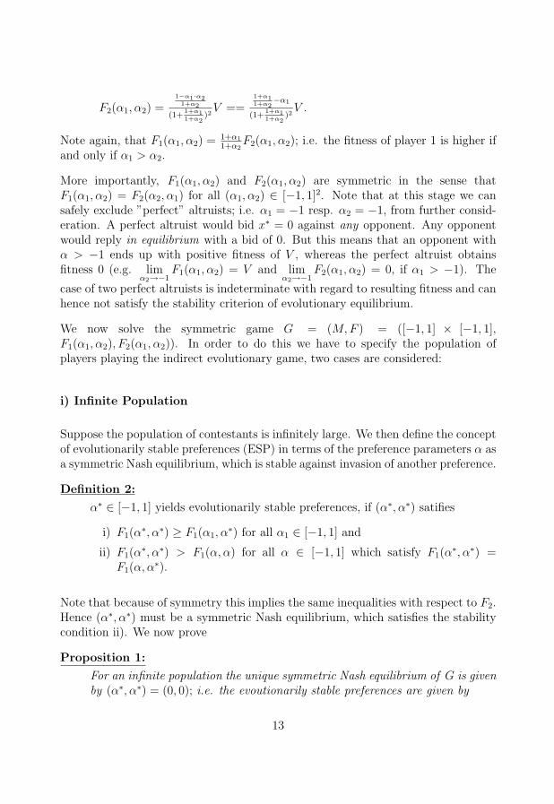
Note again, that F1(α1, α2) = 1+α1

1+α2F2(α1, α2); i.e. the fitness of player 1 is higher if

and only if α1 > α2.

More importantly, F1(α1, α2) and F2(α1, α2) are symmetric in the sense thatF1(α1, α2) = F2(α2, α1) for all (α1, α2) ∈ [−1, 1]2. Note that at this stage we cansafely exclude ”perfect” altruists; i.e. α1 = −1 resp. α2 = −1, from further consid-eration. A perfect altruist would bid x∗ = 0 against any opponent. Any opponentwould reply in equilibrium with a bid of 0. But this means that an opponent withα > −1 ends up with positive fitness of V , whereas the perfect altruist obtainsfitness 0 (e.g. lim

α2→−1F1(α1, α2) = V and lim

α2→−1F2(α1, α2) = 0, if α1 > −1). The

case of two perfect altruists is indeterminate with regard to resulting fitness and canhence not satisfy the stability criterion of evolutionary equilibrium.

We now solve the symmetric game G = (M, F ) = ([−1, 1] × [−1, 1],F1(α1, α2), F2(α1, α2)). In order to do this we have to specify the population ofplayers playing the indirect evolutionary game, two cases are considered:

i) Infinite Population

Suppose the population of contestants is infinitely large. We then define the conceptof evolutionarily stable preferences (ESP) in terms of the preference parameters α asa symmetric Nash equilibrium, which is stable against invasion of another preference.

Definition 2:

α∗ ∈ [−1, 1] yields evolutionarily stable preferences, if (α∗, α∗) satifies

i) F1(α∗, α∗) ≥ F1(α1, α

∗) for all α1 ∈ [−1, 1] and

ii) F1(α∗, α∗) > F1(α, α) for all α ∈ [−1, 1] which satisfy F1(α

∗, α∗) =F1(α, α∗).

Note that because of symmetry this implies the same inequalities with respect to F2.Hence (α∗, α∗) must be a symmetric Nash equilibrium, which satisfies the stabilitycondition ii). We now prove

Proposition 1:

For an infinite population the unique symmetric Nash equilibrium of G is givenby (α∗, α∗) = (0, 0); i.e. the evoutionarily stable preferences are given by

13

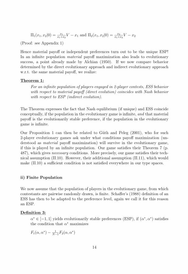
Π1(x1, x2|0) = x1

x1+x2V − x1 and Π2(x1, x2|0) = x2

x1+x2V − x2

(Proof: see Appendix 1)

Hence material payoff or independent preferences turn out to be the unique ESP!In an infinite population material payoff maximization also leads to evolutionarysuccess, a point already made by Alchian (1950). If we now compare behaviordetermined by the direct evolutionary approach and indirect evolutionary approachw.r.t. the same material payoff, we realize:

Theorem 1:

For an infinite population of players engaged in 2-player contests, ESS behaviorwith respect to material payoff (direct evolution) coincides with Nash behaviorwith respect to ESP (indirect evolution).

The Theorem expresses the fact that Nash equilibrium (if unique) and ESS coincideconceptually, if the population in the evolutionary game is infinite, and that materialpayoff is the evolutionarily stable preference, if the population in the evolutionarygame is infinite.

Our Proposition 1 can then be related to Guth and Peleg (2001), who for such2-player evolutionary games ask under what conditions payoff maximization (un-derstood as material payoff maximization) will survive in the evolutionary game,if this is played by an infinite population. Our game satisfies their Theorem 7 (p.487), which gives necessary conditions. More precisely, our game satisfies their tech-nical assumption (II.10). However, their additional assumption (II.11), which wouldmake (II.10) a sufficient condition is not satisfied everywhere in our type spaces.

ii) Finite Population

We now assume that the population of players in the evolutionary game, from whichcontestants are pairwise randomly drawn, is finite. Schaffer’s (1988) definition of anESS has then to be adapted to the preference level, again we call it for this reasonan ESP.

Definition 3:

α∗ ∈ [−1, 1] yields evolutionarily stable preferences (ESP), if (α∗, α∗) satisfiesthe condition that α∗ maximizes

F1(α, α∗) − 1N−1

F2(α, α∗)

14

Note that this condition simply results from (E), if n = 2.

So look at the following problem:

maxα1

F1(α1, α2) − 1N−1

F2(α1, α2) which reads

maxα1

1+α21+α1

−α2

(1+1+α21+α1

)2V − 1

N−1·

1+α11+α2

−α1

(1+1+α11+α2

)2V

The first-order condition of this problem is given by

(1+1+α21+α1

)2(− 1+α2(1+α1)2

)−(1+α21+α1

−α2)2·(1+ 1+α21+α1

)(− 1+α2(1+α1)2

)

(1+1+α21+α1

)4V

− 1N−1

· (1+1+α11+α2

)2( 11+α2

−1)−(1+α11+α2

−α1)(1+1+α11+α2

)·2· 11+α2

(1+1+α11+α2

)4V = 0.

Since we are looking for a symmetric solution we can set α1 = α2 = α, which yields

4(− 11+α

)−(1−α)·4·(− 11+α

)

16− 1

N−1

4( 1α+1

−1)−(1−α)·4· 11+α

16= 0.

Hence it must hold that

− 41+α

+ 4 · 1−α1+α

− 1N−1

· 41+α

+ 4N−1

+ 4N−1

· 1−α1+α

= 0

or - after multiplication by (1+α)4

-

−1 + (1 − α) − 1N−1

+ (1+α)N−1

+ 1N−1

(1 − α) = 0

−α − 1N−1

+ 1N−1

(1 + α + 1 − α) = 0

−α − 1N−1

+ 2N−1

= 0

−α + 1N−1

= 0

⇒ α = 1N−1

.

We have proven the following

Proposition 2:

For a finite population of size N the unique evolutionary stable preferences(ESP) are given by (α∗, α∗) = ( 1

N−1, 1

N−1); i.e.

Π1(x1, x2,1

N−1, 1

N−1) = x1

x1+x2V − x1 − 1

N−1( x2

x1+x2V − x2)

Π2(x1, x2,1

N−1, 1

N−1) = x2

x1+x2V − x2 − 1

N−1( x1

x1+x2V − x1).

15

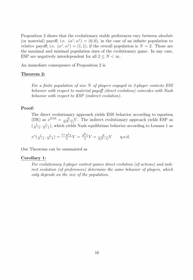
Proposition 2 shows that the evolutionary stable preferences vary between absolute(or material) payoff; i.e. (α∗, α∗) = (0, 0), in the case of an infinite population torelative payoff; i.e. (α∗, α∗) = (1, 1), if the overall population is N = 2. Those arethe maximal and minimal population sizes of the evolutionary game. In any case,ESP are negatively interdependent for all 2 ≤ N < ∞.

An immediate consequence of Proposition 2 is

Theorem 2:

For a finite population of size N of players engaged in 2-player contests ESSbehavior with respect to material payoff (direct evolution) coincides with Nashbehavior with respect to ESP (indirect evolution).

Proof:

The direct evolutionary approach yields ESS behavior according to equation(DE) as xESS = N

4(N−1)V . The indirect evolutionary approach yields ESP as

( 1N−1

, 1N−1

), which yields Nash equilibrium behavior according to Lemma 1 as

x∗( 1N−1

, 1N−1

) =1+ 1

N−1

4V =

NN−1

4V = N

4(N−1)V q.e.d.

Our Theorems can be summaried as

Corollary 1:

For evolutionary 2-player contest games direct evolution (of actions) and indi-rect evolution (of preferences) determine the same behavior of players, whichonly depends on the size of the population.

16

7 Conclusion

Our investigation has produced an ”equivalence” result: applying the direct evolu-tionary approach to Tullock’s contest model is equivalent to applying the indirectevolutionary approach. Whatever the size of the population involved in two-playercontests, the same behavior is determined by the evolutionary solutions ESS andESP. We know from Leininger (2003) and Hehenkamp et al. (2004), that in case of afinite population the former yields more aggressive - spiteful - behavior than rationalbehavior according to Nash equilibrium w.r.t. independent preferences. The latter,which combines an evolutionary process at the preference level with rational choiceat the action level, is now seen to determine negatively interdependent - spiteful- preferences, which ”rationalize” (in Nash equilibrium) this increased aggression.With a fixed population size evolutionary forces at the preference level completelyneutralize the change in the choice criterion at the action level (from ESS to NE),if preferences are endogenous to evolution.

Whether evolution works at the preference level or the action level it increases com-petition among contestants beyond the level that would apply without any evolution.With endogenous population sizes this would work towards a reduction in popula-tion sizes (because more ‘fitness‘ is dissipated in contest interaction) and hence tothe detriment of the population. This should - evolutionarily - favour groups whomanage to suppress this tendency, a topic which we want to pursue in future re-search.

17

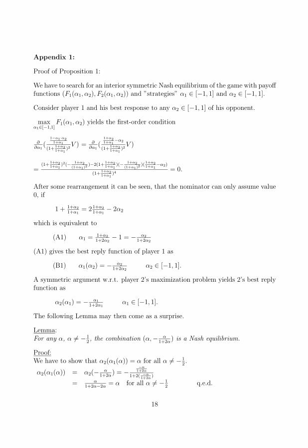
Appendix 1:

Proof of Proposition 1:

We have to search for an interior symmetric Nash equilibrium of the game with payofffunctions (F1(α1, α2), F2(α1, α2)) and ”strategies” α1 ∈ [−1, 1] and α2 ∈ [−1, 1].

Consider player 1 and his best response to any α2 ∈ [−1, 1] of his opponent.

maxα1∈[−1,1]

F1(α1, α2) yields the first-order condition

∂∂α1

(1−α1·α2

1+α1

(1+1+α21+α1

)2V ) = ∂

∂α1(

1+α21+α1

−α2

(1+1+α21+α1

)2V )

=(1+

1+α21+α1

)2(− 1+α2(1+α1)2

)−2(1+1+α21+α1

)(− 1+α2(1+α1)2

)(1+α21+α1

−α2)

(1+1+α21+α1

)4= 0.

After some rearrangement it can be seen, that the nominator can only assume value0, if

1 + 1+α2

1+α1= 21+α2

1+α1− 2α2

which is equivalent to

(A1) α1 = 1+α2

1+2α2− 1 = − α2

1+2α2

(A1) gives the best reply function of player 1 as

(B1) α1(α2) = − α2

1+2α2α2 ∈ [−1, 1].

A symmetric argument w.r.t. player 2’s maximization problem yields 2’s best replyfunction as

α2(α1) = − α1

1+2α1α1 ∈ [−1, 1].

The following Lemma may then come as a surprise.

Lemma:For any α, α �= −1

2, the combination (α,− α

1+2α) is a Nash equilibrium.

Proof:We have to show that α2(α1(α)) = α for all α �= −1

2.

α2(α1(α)) = α2(− α1+2α

) = −−α

1+2α

1+2( −α1+2α

)

= α1+2α−2α

= α for all α �= −12

q.e.d.

18

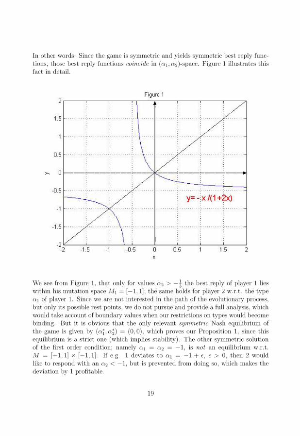
In other words: Since the game is symmetric and yields symmetric best reply func-tions, those best reply functions coincide in (α1, α2)-space. Figure 1 illustrates thisfact in detail.

We see from Figure 1, that only for values α2 > −13

the best reply of player 1 lieswithin his mutation space M1 = [−1, 1]; the same holds for player 2 w.r.t. the typeα1 of player 1. Since we are not interested in the path of the evolutionary process,but only its possible rest points, we do not pursue and provide a full analysis, whichwould take account of boundary values when our restrictions on types would becomebinding. But it is obvious that the only relevant symmetric Nash equilibrium ofthe game is given by (α∗

1, α∗2) = (0, 0), which proves our Proposition 1, since this

equilibrium is a strict one (which implies stability). The other symmetric solutionof the first order condition; namely α1 = α2 = −1, is not an equilibrium w.r.t.M = [−1, 1] × [−1, 1]. If e.g. 1 deviates to α1 = −1 + ε, ε > 0, then 2 wouldlike to respond with an α2 < −1, but is prevented from doing so, which makes thedeviation by 1 profitable.

19

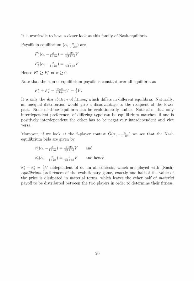
It is worthwile to have a closer look at this family of Nash-equilibria.

Payoffs in equilibrium (α, α1+2α

) are

F ∗1 (α,− α

1+2α) = 1+2α

4(1+α)V

F ∗2 (α,− α

1+2α) = 1

4(1+α)V

Hence F ∗1 ≥ F ∗

2 ⇔ α ≥ 0.

Note that the sum of equilibrium payoffs is constant over all equilibria as

F ∗1 + F ∗

2 = 2+2α4(1+α)

V = 12V .

It is only the distribution of fitness, which differs in different equilibria. Naturally,an unequal distribution would give a disadvantage to the recipient of the lowerpart. None of these equilibria can be evolutionarily stable. Note also, that onlyinterdependent preferences of differing type can be equilibrium matches; if one ispositively interdependent the other has to be negatively interdependent and viceversa.

Moreover, if we look at the 2-player contest G(α,− α1+2α

) we see that the Nashequilibrium bids are given by

x∗1(α,− α

1+2α) = 1+2α

4(1+α)V and

x∗2(α,− α

1+2α) = 1

4(1+α)V and hence

x∗1 + x∗

2 = 12V independent of α. In all contests, which are played with (Nash)

equilibrium preferences of the evolutionary game, exactly one half of the value ofthe prize is dissipated in material terms, which leaves the other half of materialpayoff to be distributed between the two players in order to determine their fitness.

20

References

[1] Alchian, A., 1950, Uncertainty, Evolution and Economic Theory, Journal ofPolitical Economy 58, 211-221

[2] Congleton, R., Hillman, A. and K. Konrad (eds.), 2008, 40 years of Researchon Rent Seeking, Volumes 1 and 2, Springer Verlag, Heidelberg

[3] Guth, W. and B. Peleg, 2001, When will payoff maximization survive? Anindirect evolutionary analysis, Journal of Evolutionary Economics, 11, 479-499

[4] Guth, W. and M. Yaari, 1992, An evolutionary approach to explaining re-ciprocal behavior in a simple strategic game, in: ”Explaining Process andchange - Approaches to Evolutionary Economics” (ed. Witt, U.), university ofMichigan Press, Ann Arbor, 23-34

[5] Guse, T. and B. Hehenkamp, 2006, The strategic advantage of interdependentpreferences in rent-seeking contests, Public Choice, 129, 323-352

[6] Hehenkamp, B., 2007, Nash vs. Evolutionary Equilibrium, in ”Interdepen-dent Preferences in Strategic Interaction”, Habitation Thesis, University ofDortmund, unpublished

[7] Hehenkamp, B., Leininger, W. and A. Possajennikov, 2004, EvolutionaryEquilibrium in Tullock Contests: Spite and Overdissipation, European Jour-nal of Political Economy, 20, 1045-105

[8] Kockesen, L., Ok, E. and R. Sethi, 2000a, Evolution of interdependent pref-erences in aggregative games, Games and Economic Behavior, 31, 303-310

[9] Kockesen, L., Ok, E. and R. Sethi, 2000b, The static advantage of negativelyinterdependent preferences, Journal of Economic Theory, 92, 274-299

[10] Leininger, W., 2006, Fending off one means fending off all: evolutionary stabil-ity in quasi-submodular aggregative games, Economic Theory, 2006, 713-719

[11] Leininger, W., 2003, On Evolutionarily Stable Behavior in Contests, Eco-nomics of Governance, 4, 177-186

[12] Lockard, A. and G. Tullock (eds.), 2001, Efficient Rent-seeking: Chronicle ofan Intellectual Quagmire, Kluwer Academic Publishering, Boston

[13] Maynard Smith, J., 1974, The Theory of Games and the Evolution of AnimalConflicts, Journal of Theoretical Biology 47, 209-221

21

[14] Schaffer, M., 1988, Evolutionarily Stable Strategies for a finite Population anda variable Contest Size, Journal of Theoretical Biology 132, 469-478

[15] Schmidt, F., 2007, A Note on Evolutionary Equilibria in Endogenous PrizeContests, Discussion Paper, University of Mainz

[16] Tullock, G., 1980, Efficient Rent-Seeking, in: Buchanan, Tollison and Tullock(eds.), Toward a Theory of the Rent-seeking Society, Texas A & M UniversityPress, 3-15

[17] Warneryd, K., 2008, The Evolution of Preferences for Conflict, mimeo, Stock-holm School of Economics

[18] Weibull, J., 1995, Evolutionary Game Theory, MIT Press, Cambridge Mas-sachusetts

22