1

WKB approximation: particle decay Masatsugu Sei Suzuki

Department of Physics, SUNY at Binghamton (Date: January 13, 2012)

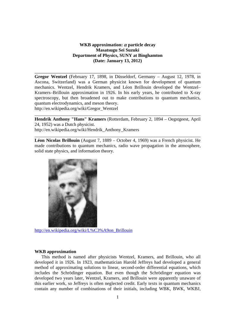
________________________________________________________________________ Gregor Wentzel (February 17, 1898, in Düsseldorf, Germany – August 12, 1978, in Ascona, Switzerland) was a German physicist known for development of quantum mechanics. Wentzel, Hendrik Kramers, and Léon Brillouin developed the Wentzel–Kramers–Brillouin approximation in 1926. In his early years, he contributed to X-ray spectroscopy, but then broadened out to make contributions to quantum mechanics, quantum electrodynamics, and meson theory. http://en.wikipedia.org/wiki/Gregor_Wentzel ________________________________________________________________________ Hendrik Anthony "Hans" Kramers (Rotterdam, February 2, 1894 – Oegstgeest, April 24, 1952) was a Dutch physicist. http://en.wikipedia.org/wiki/Hendrik_Anthony_Kramers ________________________________________________________________________ Léon Nicolas Brillouin (August 7, 1889 – October 4, 1969) was a French physicist. He made contributions to quantum mechanics, radio wave propagation in the atmosphere, solid state physics, and information theory.

http://en.wikipedia.org/wiki/L%C3%A9on_Brillouin WKB approximation

This method is named after physicists Wentzel, Kramers, and Brillouin, who all developed it in 1926. In 1923, mathematician Harold Jeffreys had developed a general method of approximating solutions to linear, second-order differential equations, which includes the Schrödinger equation. But even though the Schrödinger equation was developed two years later, Wentzel, Kramers, and Brillouin were apparently unaware of this earlier work, so Jeffreys is often neglected credit. Early texts in quantum mechanics contain any number of combinations of their initials, including WBK, BWK, WKBJ,

2

JWKB and BWKJ. The important contribution of Jeffreys, Wentzel, Kramers and Brillouin to the method was the inclusion of the treatment of turning points, connecting the evanescent and oscillatory solutions at either side of the turning point. For example, this may occur in the Schrödinger equation, due to a potential energy hill. (from http://en.wikipedia.org/wiki/WKB_approximation) ________________________________________________________________________ 1. Classical limit

Change in the wavelength over the distance x

dxdx

d .

When x

dx

d .

In the classical domain,

dx

d or 1

dx

d,

which is the criterion of the classical behavior. 2. WKB approximation

The quantum wavelength does not change appreciably over the distance of one wavelength. We start with the de Broglie wave length given by

h

p

)(2

1 2 xVpm

or

)]([22

2 xVmh

p

,

or

)((2 xVmp .

3

Then we get

])(

[22 32

dx

xdVm

dx

dh ,

or

dx

xdV

p

mh

dx

xdV

p

h

h

m

dx

xdV

h

m

dx

d )()()(3

3

23

2

.

When 1dx

d, we have

1)(

3

dx

xdV

p

mh (classical approximation)

If dV/dx is small, the momentum is large, or both, the above inequality is likely to be satisfied Around the turning point, p(x) = 0. |dV/dx| is very small when V(x) is a slowly changing function of x. Now we consider the WKB approximation,

)()(2

)(2

22

xxVxm

x

.

When 0V ,

ipx

ikx AeAex )( . If the potential V is slowly varying function of x, we can assume that

)()(

xSi

Aex ,

.....)(!3

)(!2

)(!1

)()( 3

3

2

2

10 xSxSxSxSxS

.

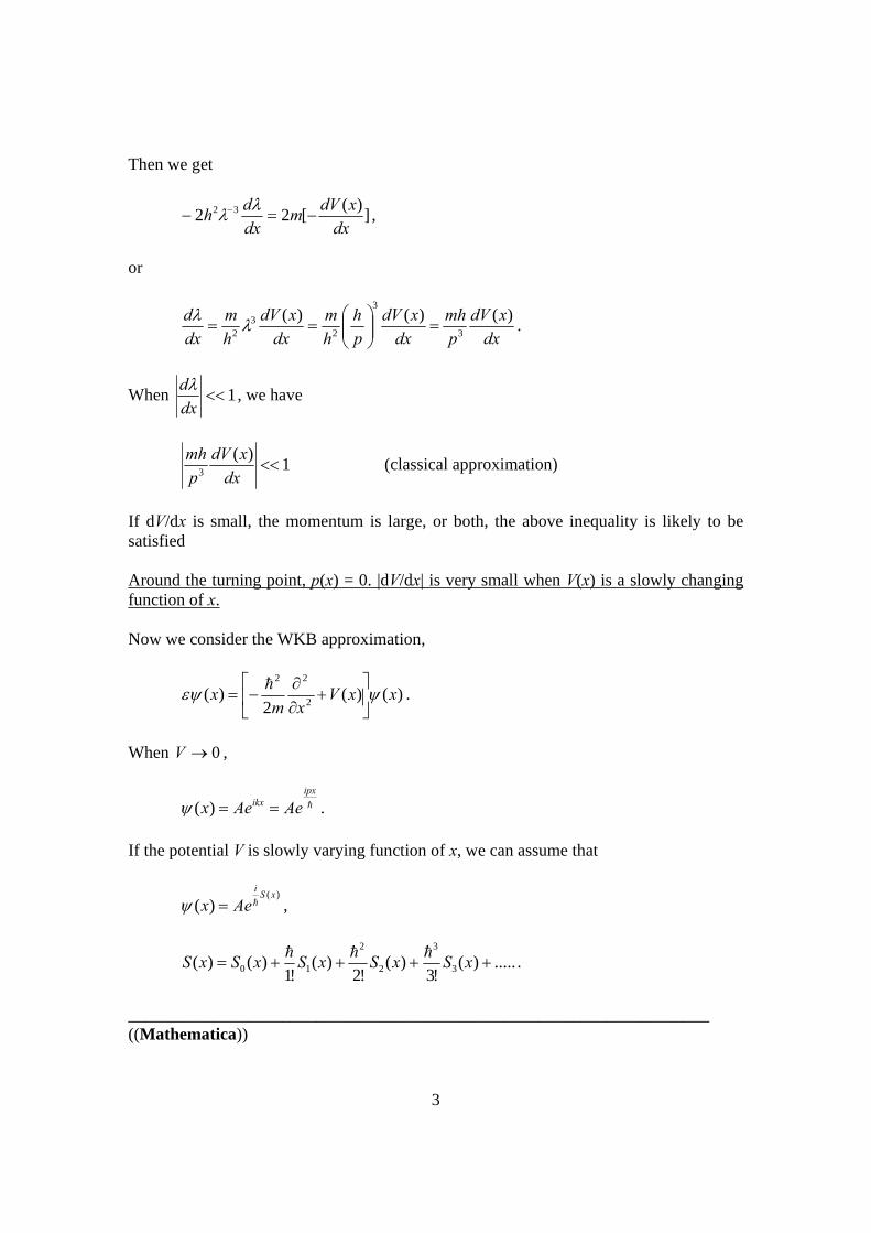
____________________________________________________________________ ((Mathematica))

4

WKB approximation

eq1 —2

2 mDx, x, 2 Vx x ∂ x;

rule1 Exp—

S & ;

eq2 eq1 . rule1 Simplify

Sx

— 2 m ∂ 2 m Vx Sx2 — Sx2 m

rule2

S

S0 — S1 —2

2S2

—3

3S3 —4

4S4 & ;

eq3 2 ∂ m 2 m Vx Sx2 — Sx;

eq4 eq3 . rule2 Expand;

list1 Tablen, Coefficienteq4, —, n, n, 0, 6 Simplify;

TableForm

0 2 m ∂ 2 m Vx S0x2

1 2 S0x S1x S0x2 S1x2 S0x S2x S1x3 S1x S2x 1

3S0x S3x 1

2 S2x

4 112

3 S2x2 4 S1x S3x S0x S4x 2 S3x5 1

244 S2x S3x 2 S1x S4x S4x

6 172

2 S3x2 3 S2x S4x

_______________________________________________________________________ For each power of ħ, we have

0)]('[)(22 20 xSxmVm ,

5

)(")(')('2 010 xiSxSxS ,

)(")(')(')]('[ 120

21 xiSxSxSxS ,

..................................................................................................................................... (a) Derivation of )(0 xS

)()]([2)]('[ 22

0 xpxVmxS ,

where

)]([2)(2 xVmxp , or

)()('0 xpxS ,

or

x

x

dxxpxS0

)()(0 .

Since )()( xkxp ,

x

x

dxxkxS0

)()(0 .

(b) Derivation of )(1 xS

)(")(')('2 010 xiSxSxS ,

)('

)('

2)('2

)(")('

0

0

0

01 xS

xSdx

di

xS

xiSxS ,

which is independent of sign.

)](ln[2

)]('ln[2

)(')( 011 xki

xSi

dxxSxS ,

or

6

2/1

1 )](ln[)](ln[2

1)( xkxkxiS ,

or

)(

1)(1

xke xiS

.

(c) Derivation of )(2 xS

)(")(')(')]('[ 1202

1 xiSxSxSxS ,

)('

)]('[)(")('

0

211

2 xS

xSxiSxS

.

Then the WKB solution is given by

..)](ln[2

)(

.....)(!3

)(!2

)(!1

)()(

0

3

3

2

2

10

xki

dxxk

xSxSxSxSxS

x

x

The wave function has the form

)])(exp("))(exp('))][(ln(2

1exp[)(

00

x

x

x

x

dxxkiBdxxkiAxkx ,

or

))(exp()(

))(exp()(

))(exp()(

'))(exp(

)(

')(

00

00

x

x

x

x

x

x

x

x

dxxkixk

Bdxxki

xk

A

dxxkixk

Bdxxki

xk

Ax

.

where we put

'A

A , 'B

B

3. The probability current density

7

We now consider the case of B = 0.

))(exp()(

)(0

x

x

dxxkixk

Ax .

The probability is obtained as

mv

A

xk

AxxxP

22

)()()(*)( ,

where mvxk )( . The probability current density is

22

2A

mmv

AvvJ

.

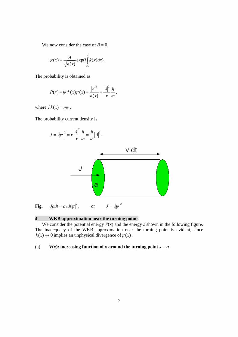
Fig. 2avdtJadt , or

2vJ

4. WKB approximation near the turning points

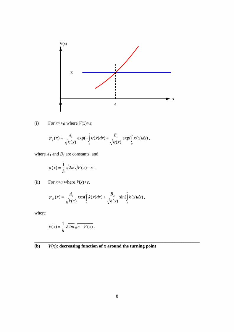
We consider the potential energy V(x) and the energy shown in the following figure. The inadequacy of the WKB approximation near the turning point is evident, since

0)( xk implies an unphysical divergence of )(x . (a) V(x): increasing function of x around the turning point x = a

8

Vx

xaO

E

(i) For x>>a where V(x)>,

))(exp()(

))(exp()(

)( 11 x

a

x

a

I dxxx

Bdxx

x

Ax

,

where A1 and B1 are constants, and

)(21

)( xVmx

,

(ii) For x<a where V(x)<,

))(sin()(

))(cos()(

)( 22 a

x

a

x

II dxxkxk

Bdxxk

xk

Ax ,

where

)(21

)( xVmxk

.

________________________________________________________________________ (b) V(x): decreasing function of x around the turning point

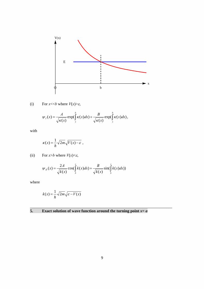
9

Vx

xbO

E

(i) For x<<b where V(x)>,

))(exp()(

))(exp()(

)( b

x

b

x

I dxxx

Bdxx

x

Ax

,

with

)(21

)( xVmx

,

(ii) For x>b where V(x)<,

)))(sin()(

))(cos()(

2)(

x

b

x

b

II dxxkxk

Bdxxk

xk

Ax

where

)(21

)( xVmxk

_______________________________________________________________________ 5. Exact solution of wave function around the turning point x= a

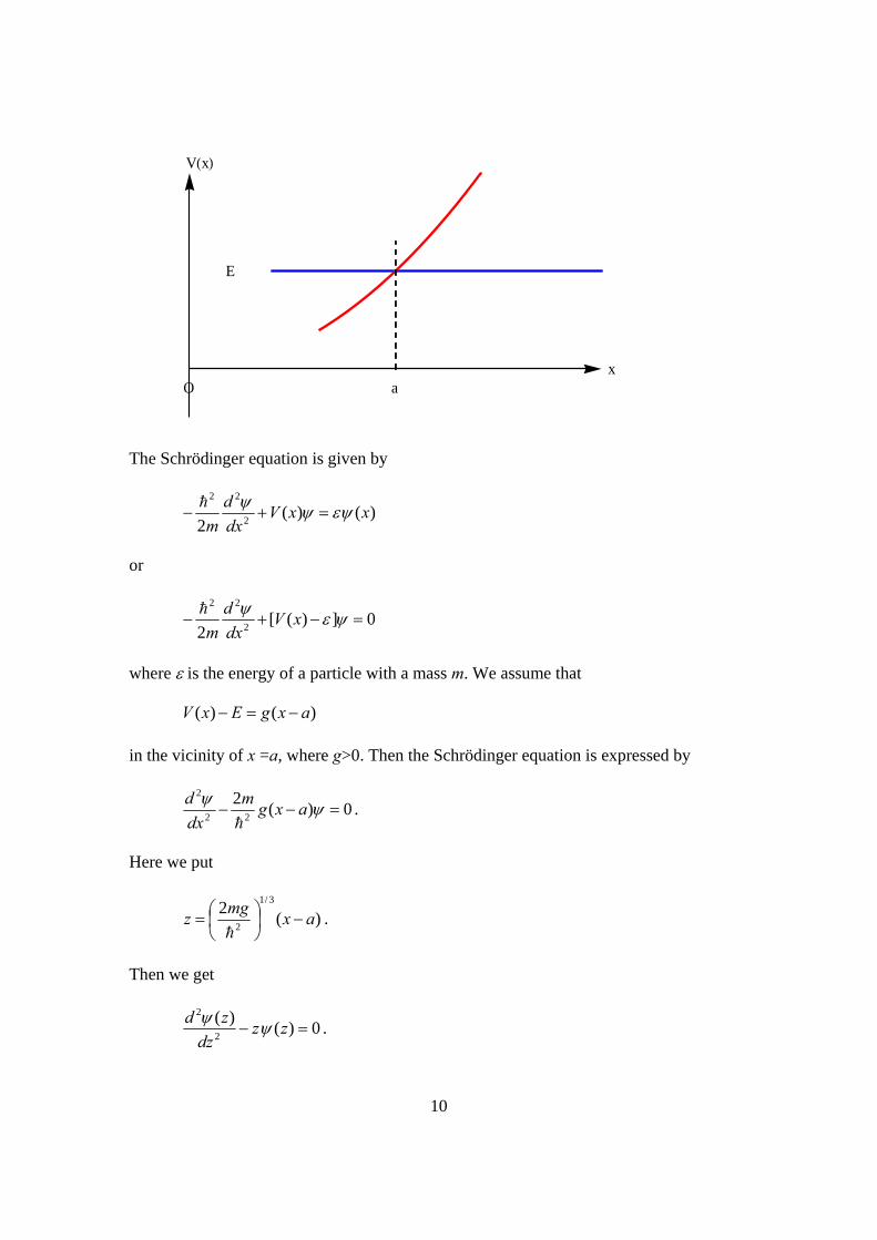
10

Vx

xaO

E

The Schrödinger equation is given by

)()(2 2

22

xxVdx

d

m

or

0])([2 2

22

xV

dx

d

m

where is the energy of a particle with a mass m. We assume that

)()( axgExV in the vicinity of x =a, where g>0. Then the Schrödinger equation is expressed by

0)(2

22

2

axg

m

dx

d

.

Here we put

)(2

3/1

2ax

mgz

.

Then we get

0)()(

2

2

zzdz

zd .

11

The solution of this equation is given by

)()(2)( 21 zBCzACz ii

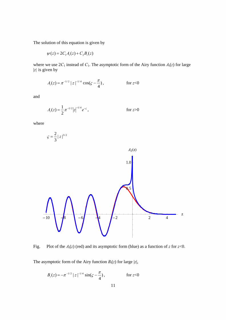
where we use 2C1 instead of C1. The asymptotic form of the Airy function Ai(z) for large |z| is given by

)4

cos(||)( 4/12/1 zzAi , for z<0

and

ezzAi

4/12/1

2

1)( , for z>0

where

2/3||3

2z

-10 -8 -6 -4 -2 2 4z

0.5

1.0

Aiz

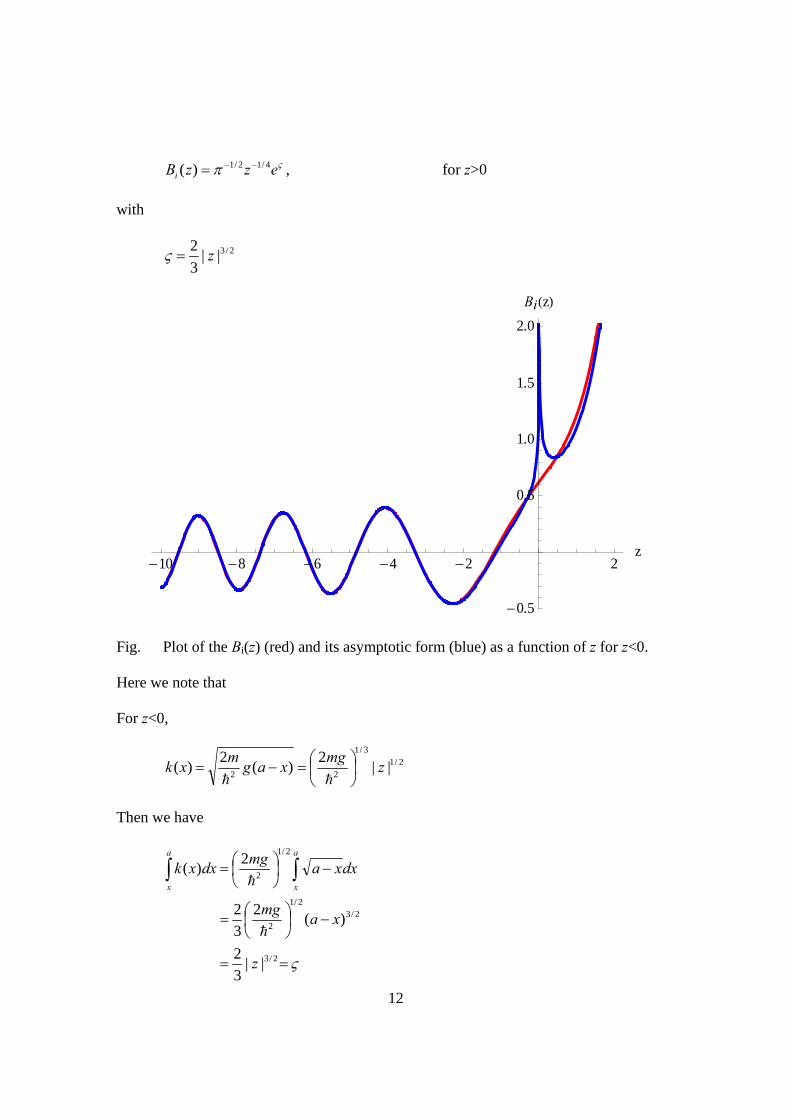
Fig. Plot of the Ai(z) (red) and its asymptotic form (blue) as a function of z for z<0. The asymptotic form of the Airy function Bi(z) for large |z|,

)4

sin(||)( 4/12/1 zzBi , for z<0

12

ezzBi

4/12/1)( , for z>0

with

2/3||3

2z

-10 -8 -6 -4 -2 2z

-0.5

0.5

1.0

1.5

2.0

Biz

Fig. Plot of the Bi(z) (red) and its asymptotic form (blue) as a function of z for z<0. Here we note that For z<0,

2/13/1

22||

2)(

2)( z

mgxag

mxk

Then we have

2/3

2/32/1

2

2/1

2

||3

2

)(2

3

2

2)(

z

xamg

dxxamg

dxxka

x

a

x

13

For z>0,

2/13/1

22||

2)(

2)( z

mgaxg

mx

we have

2/3

2/32/1

2

2/1

2

||3

2

)(2

3

2

2)(

z

axmg

dxaxmg

dxxx

a

x

a

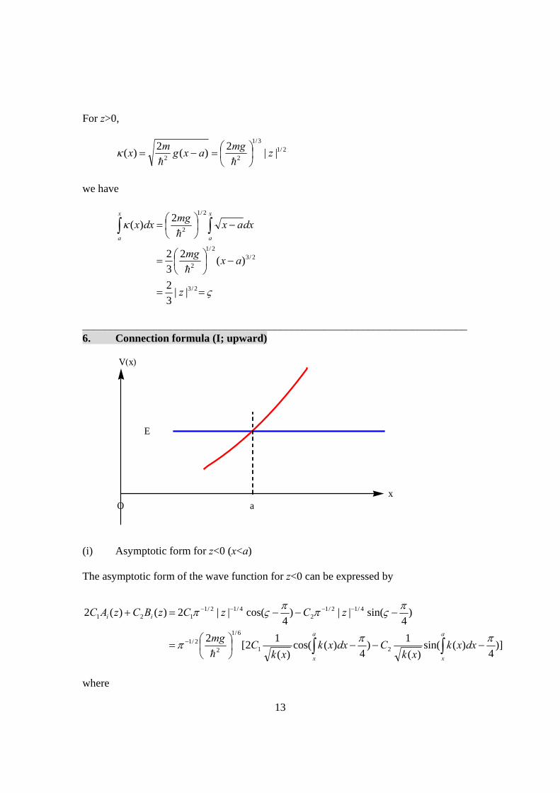
______________________________________________________________________ 6. Connection formula (I; upward)

Vx

xaO

E

(i) Asymptotic form for z<0 (x<a) The asymptotic form of the wave function for z<0 can be expressed by

)]4

)(sin()(

1)

4)(cos(

)(

12[

2

)4

sin(||)4

cos(||2)()(2

21

6/1

22/1

4/12/12

4/12/1121

a

x

a

x

ii

dxxkxk

Cdxxkxk

Cmg

zCzCzBCzAC

where

14

2/3||3

2)( zdxxk

a

x

, 2/13/1

2||

2)( z

mgxk

.

(ii) The asymptotic form for z>0; The asymptotic form of the wave function for z>0 can be expressed by

)])(exp()(

1))(exp(

)(

1[

2

)()(2

21

6/1

22/1

4/12/12

4/12/1121

x

a

x

a

ii

dxxx

Cdxxx

Cmg

ezCezCzBCzAC

where

2/3||3

2)( zdxx

x

a

, 2/13/1

2||

2)( z

mgx

.

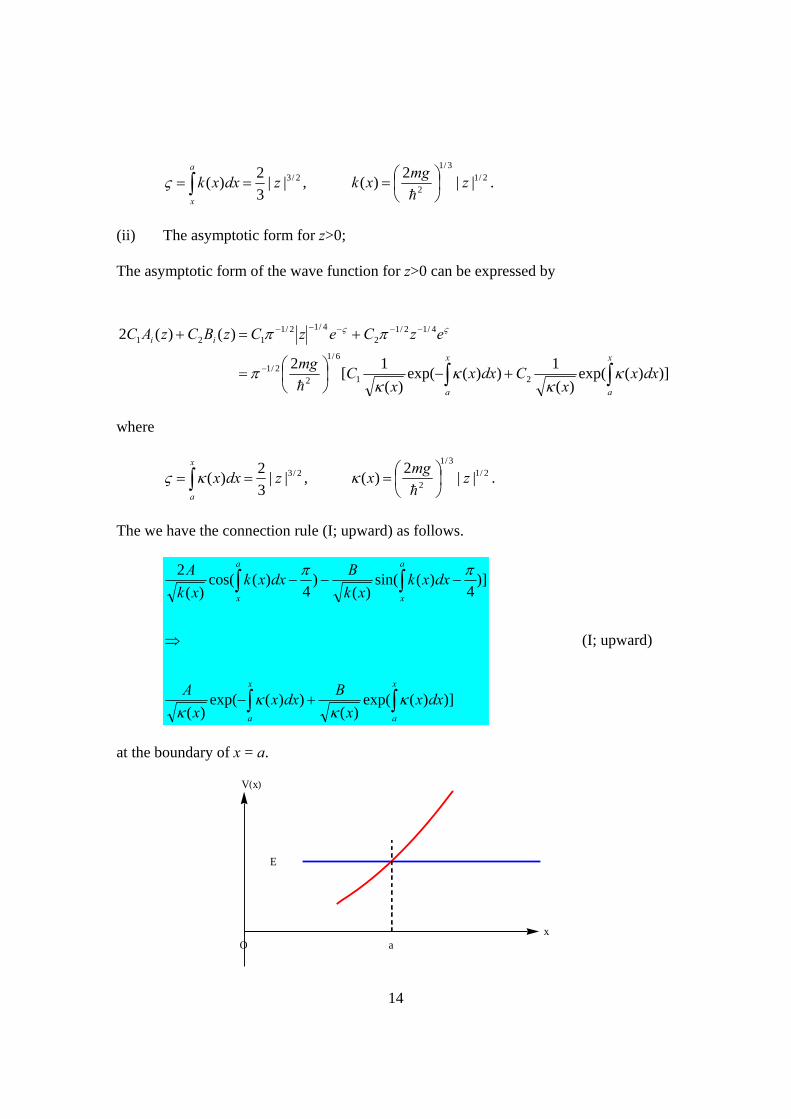
The we have the connection rule (I; upward) as follows.

)])(exp()(

))(exp()(

)]4

)(sin()(

)4

)(cos()(

2

x

a

x

a

a

x

a

x

dxxx

Bdxx

x

A

dxxkxk

Bdxxk

xk

A

(I; upward)

at the boundary of x = a.

Vx

xaO

E

15

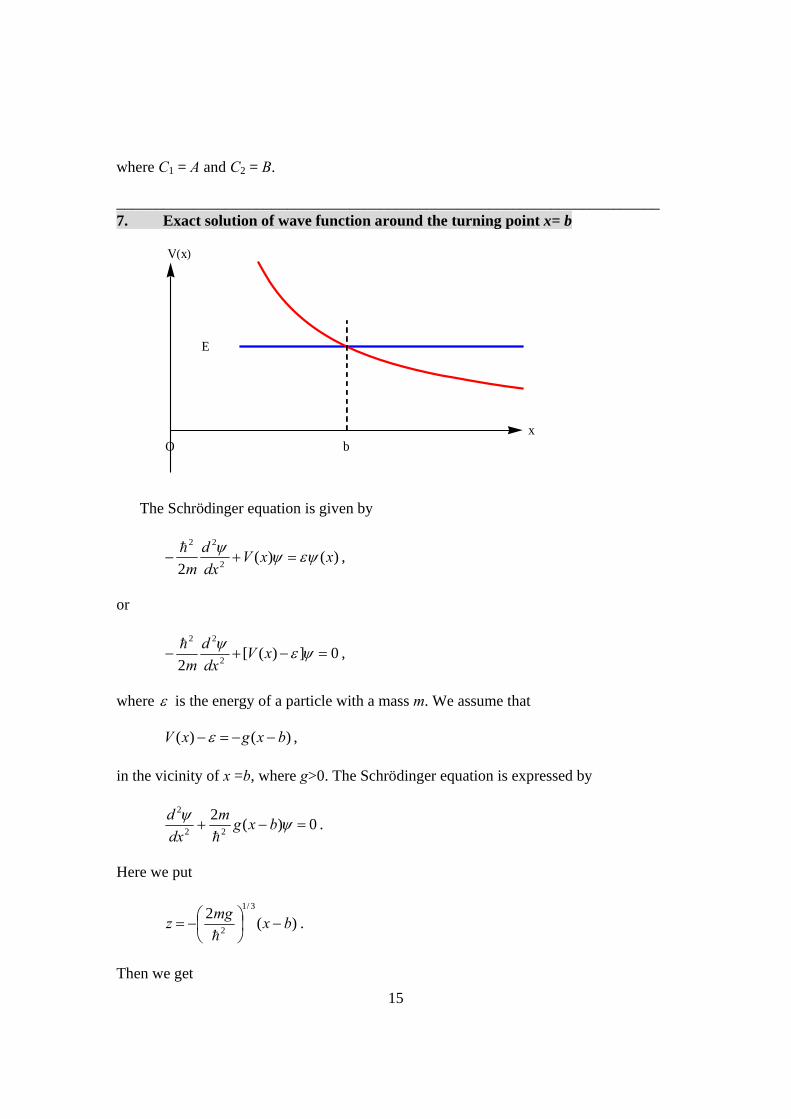
where C1 = A and C2 = B. ______________________________________________________________________ 7. Exact solution of wave function around the turning point x= b

Vx

xbO

E

The Schrödinger equation is given by

)()(2 2

22

xxVdx

d

m

,

or

0])([2 2

22

xV

dx

d

m

,

where is the energy of a particle with a mass m. We assume that

)()( bxgxV , in the vicinity of x =b, where g>0. The Schrödinger equation is expressed by

0)(2

22

2

bxg

m

dx

d

.

Here we put

)(2

3/1

2bx

mgz

.

Then we get

16

0)()(

2

2

zzdz

zd .

The solution of this equation is given by

)()(2)( 21 zBCzACz ii .

We note the following. (i) For z<0 (x>b) k(x) is expressed by

2/13/1

22||

2)(

2)( z

mgbxg

mxk

,

2/32/3

2/1

2

2/1

2||

3

2)(

2

3

22)( zbx

mgdxbx

mgdxxk

x

b

x

b .

(ii) For z>0 (x<b), where >V(x) (x) is expressed by

2/13/1

2

22

2

)(2

)]([2

)(

zmg

xbgm

xVm

x

2/32/32/1

2

2/1

2 3

2)(

2

3

22)( zxb

mgdxxb

mgdxx

b

x

b

x

__________________________________________________________________ 8. Connection formula-II (downward)

The asymptotic form for z<0;

)]4

)(sin()(

1

)4

)(cos()(

12[

2

)4

sin(||)4

cos(||2)()(2

2

1

6/1

22/1

4/12/12

4/12/1121

x

b

x

b

ii

dxxkxk

C

dxxkxk

Cmg

zCzCzBCzAC

17

The asymptotic form for z>0;

)])(exp()(

1

))(exp()(

1[

2

)()(2

2

1

6/1

22/1

4/12/12

4/12/1121

b

x

b

x

ii

dxxx

C

dxxx

Cmg

ezCezCzBCzAC

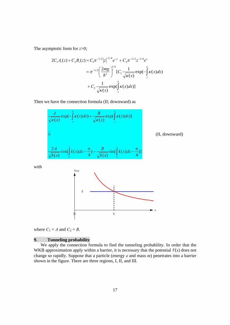
Then we have the connection formula (II; downward) as

)]4

)(sin()(

)4

)(cos()(

2

)])(exp()(

))(exp()(

x

b

x

b

b

x

b

x

dxxkxk

Bdxxk

xk

A

dxxx

Bdxx

x

A

(II, downward)

with

Vx

xbO

E

where C1 = A and C2 = B. 9. Tunneling probability

We apply the connection formula to find the tunneling probability. In order that the WKB approximation apply within a barrier, it is necessary that the potential V(x) does not change so rapidly. Suppose that a particle (energy and mass m) penetrates into a barrier shown in the figure. There are three regions, I, II, and III.

18

ba

I II III

Vx

E

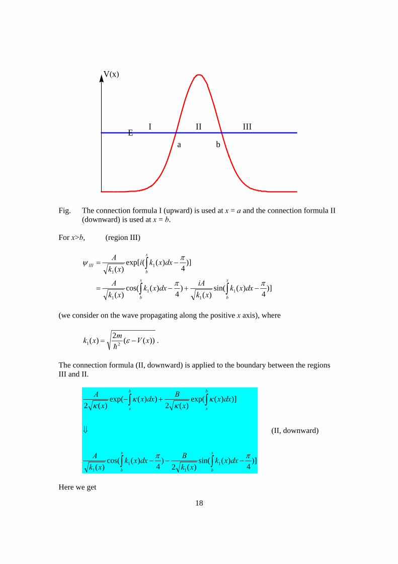
Fig. The connection formula I (upward) is used at x = a and the connection formula II

(downward) is used at x = b. For x>b, (region III)

)]4

)(sin()(

)4

)(cos()(

)]4

)((exp[)(

1

1

1

1

1

1

x

b

x

b

x

b

III

dxxkxk

iAdxxk

xk

A

dxxkixk

A

(we consider on the wave propagating along the positive x axis), where

))((2

)(21 xVm

xk

.

The connection formula (II, downward) is applied to the boundary between the regions III and II.

)]4

)(sin()(2

)4

)(cos()(

)])(exp()(2

))(exp()(2

1

1

1

1

x

b

x

b

b

x

b

x

dxxkxk

Bdxxk

xk

A

dxxx

Bdxx

x

A

(II, downward)

Here we get

19

iAB 2 .

Then we get the wave function of the region II,

)]4

)(sin()(

)4

)(cos()(

)])(exp()(

))(exp()(2

1

1

1

1

x

b

x

b

III

b

x

b

x

II

dxxkxk

iAdxxk

xk

A

dxxx

iAdxx

x

A

or

))(exp(2)(

))(exp(1

)(

)])()(exp()(

))()(exp()(2

x

a

x

a

x

a

b

a

b

a

x

a

II

dxxr

x

Adxx

rx

iA

dxxdxxx

iAdxxdxx

x

A

where

))((2

)(2

xVm

x

,

and

))(exp( b

a

dxxr ,

Next, the connection formula (I; upward) is applied to the boundary between the regions II and I.

20

)])(exp()(

))(exp()(

)]4

)(sin()(

)4

)(cos()(

22

2

2

2

x

a

x

a

a

x

a

x

dxxx

Ddxx

x

C

dxxkxk

Ddxxk

xk

C

(I; upward)

Here we get

riAC

1 ,

rA

D2

.

Then we have the wave function of the region I,

)]}4

)((exp[)]4

)(({exp[4)(

)]}4

)((exp[)]4

)(({exp[1

)(

)]4

)(sin()(2

)4

)(cos(1

)(

2

22

2

22

2

2

2

2

2

a

x

a

x

a

x

a

x

a

x

a

x

I

dxxkidxxkiir

xk

A

dxxkidxxkirxk

iA

dxxkrxk

A

dxxkrxk

iA

or

)]}4

)((exp[))4

1()]

4)((exp[)

4

1{(

)(

)]}4

)((exp[)1

4()]

4)((exp[)

1

4{(

)(

22

2

22

2

x

a

x

a

a

x

a

x

I

dxxkir

rdxxki

r

rxk

iA

dxxkir

rdxxki

r

r

xk

iA

The first term corresponds to that of the reflected wave and the second term corresponds to that of the incident wave. Then the tunneling probability is

21

))(2exp()

41

(

1 2

2

b

a

dxxrr

r

T

where

))(exp( b

a

dxxr

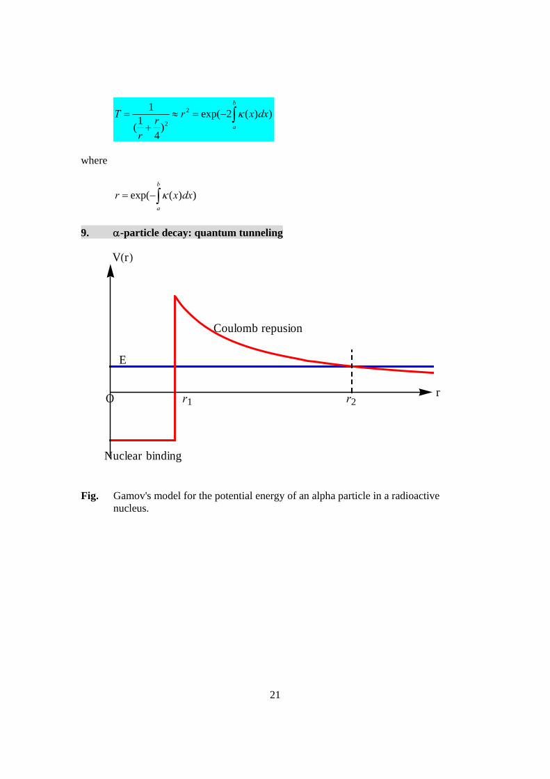
9. -particle decay: quantum tunneling

r1 r2

Coulomb repusion

Nuclear binding

Vr

rO

E

Fig. Gamov's model for the potential energy of an alpha particle in a radioactive

nucleus.

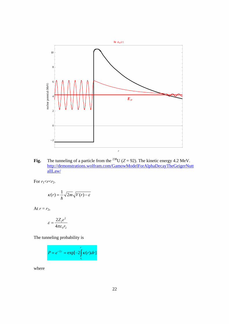
22

-2

0

2

4

6

8

10

r

nucl

ear

pote

ntia

lMeV

Re yar

Ea

Fig. The tunneling of a particle from the 238U (Z = 92). The kinetic energy 4.2 MeV.

http://demonstrations.wolfram.com/GamowModelForAlphaDecayTheGeigerNuttallLaw/

For r1<r<r2.

)(21

)( rVmr

At r = r2,

20

21

4

2

r

eZ

The tunneling probability is

])(2exp[1

2 r

r

drreP

where

23

])1([arccos2

])(arccos[2

12

)(2

)(

2

1

2

1

2

12

1212

12

22

1

2

1

2

1

r

r

r

r

r

rr

m

rrrr

rr

m

drr

rm

drrVm

drr

r

r

r

r

r

r

where m is the mass of -particle (= 4.001506179125 u). fm = 10-15 m (fermi).

The quantity P gives the probability that in one trial an particle will penetrate the barrier. The number of trials per second could estimated to be

12r

vN

if it were assumed that a particle is bouncing back and forth with velocity v inside the nucleus of diameter 2r1. Then the probability per second that nucleus will decay by emitting a particle, called the decay rate R, would be

2

12 e

r

vR

((Example))

We consider the particle emission from 238U nucleus (Z = 92), which emits a K = 4.2 MeV particle. The a particle is contained inside the nuclear radius r1 = 7.0 fm (fm = 10-15 m). (i) The distance r2: From the relation

20

2

4

2

r

ZeK

we get

r2 = 63.08 fm. (ii) The velocity of a particle inside the nucleus, v:

24

From the relation

21 2

1vmK

where m is the mass of the a particle; m = 4.001506179 u, we get

v = 1.42318 x 107 m/s (iii) The value of :

])(arccos[2

1212

12 rrr

r

rr

mK

=51.8796

(iv) The decay rate R:

2

12 e

r

vR = 8.813 x 10-25.

((Mathematica))

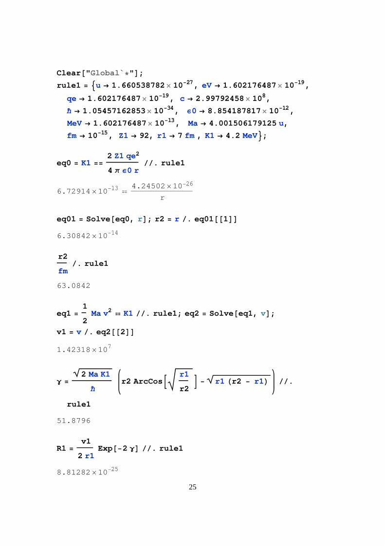
25

Clear"Global`";

rule1 u 1.660538782 1027, eV 1.602176487 1019,

qe 1.602176487 1019, c 2.99792458 108,

— 1.05457162853 1034, 0 8.854187817 1012,

MeV 1.602176487 1013, Ma 4.001506179125 u,

fm 1015, Z1 92, r1 7 fm , K1 4.2 MeV;

eq0 K1 2 Z1 qe2

4 0 r. rule1

6.729141013 4.245021026

r

eq01 Solveeq0, r; r2 r . eq0116.308421014

r2

fm. rule1

63.0842

eq1 1

2Ma v2 K1 . rule1; eq2 Solveeq1, v;

v1 v . eq221.42318107

2 Ma K1

—r2 ArcCos r1

r2 r1 r2 r1 .

rule1

51.8796

R1 v1

2 r1Exp2 . rule1

8.812821025

26

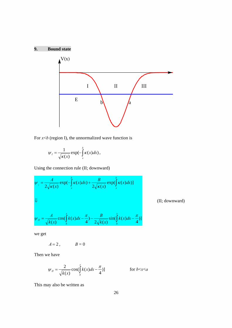
9. Bound state

ab

I II III

Vx

E

For x<b (region I), the unnormalized wave function is

))(exp()(

1b

x

I dxxx

,

Using the connection rule (II; downward)

)]4

)(sin()(2

)4

)(cos()(

)])(exp()(2

))(exp()(2

x

b

x

b

II

b

x

b

x

dxxkxk

Bdxxk

xk

A

dxxx

Bdxx

x

AI

(II; downward)

we get

2A , B = 0 Then we have

)]4

)(cos()(

2 x

b

II dxxkxk

for b<x<a

This may also be written as

27

]4

))(sin[])(cos[)(

2

]4

))(cos[])(sin[)(

2

]4

))()(sin[)(

2

]24

))()(cos[)(

2

)]4

)()(cos()(

2)]

4)(cos(

)(

2

a

x

a

b

a

x

a

b

a

x

a

b

a

x

a

b

a

x

a

b

x

b

II

dxxkdxxkxk

dxxkdxxkxk

dxxkdxxkxk

dxxkdxxkxk

dxxkdxxkxk

dxxkxk

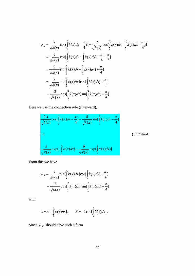
Here we use the connection rule (I, upward),

)])(exp()(

))(exp()(

)4

)(sin()(

)4

)(cos()(

2

x

a

x

a

a

x

a

x

dxxx

Bdxx

x

A

dxxkxk

Bdxxk

xk

A

(I; upward)

From this we have

]4

))(sin[])(cos[)(

2

]4

))(cos[])(sin[)(

2

a

x

a

b

a

x

a

b

II

dxxkdxxkxk

dxxkdxxkxk

with

])(sin[a

b

dxxkA , ])(cos[2 a

b

dxxkB .

Since III should have such a form

28

))(exp()(

x

a

III dxxx

A

for x>a. Then we need the condition that

0])(cos[2 a

b

dxxkB ,

or

)2

1()( ndxxk

a

b

or

)2

1()( ndxxp

a

b

,

where n = 0, 1, 2, ... 10. Simple harmonics

We consider a simple harmonics,

2200

22 2)2

1(2))((2)( xxmxmmxVmxp

where

20

0

2

mx .

Then we get

02

0

0

20

0

0

2200

2

2

1

422)(

00

0

mm

xmdxxxmdxxp

xx

x

When

)2

1()(

0

ndxxpa

x

29

we have

)2

1(

0

n ,

or

)2

1( n

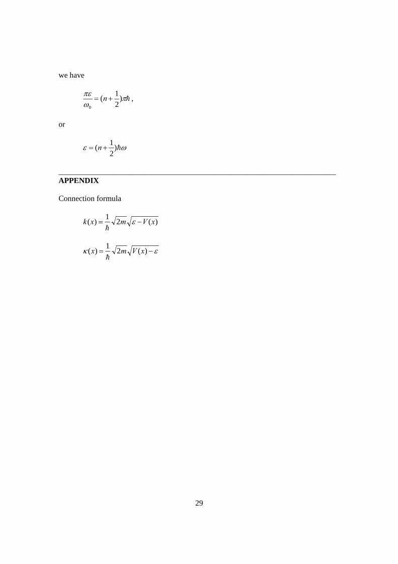
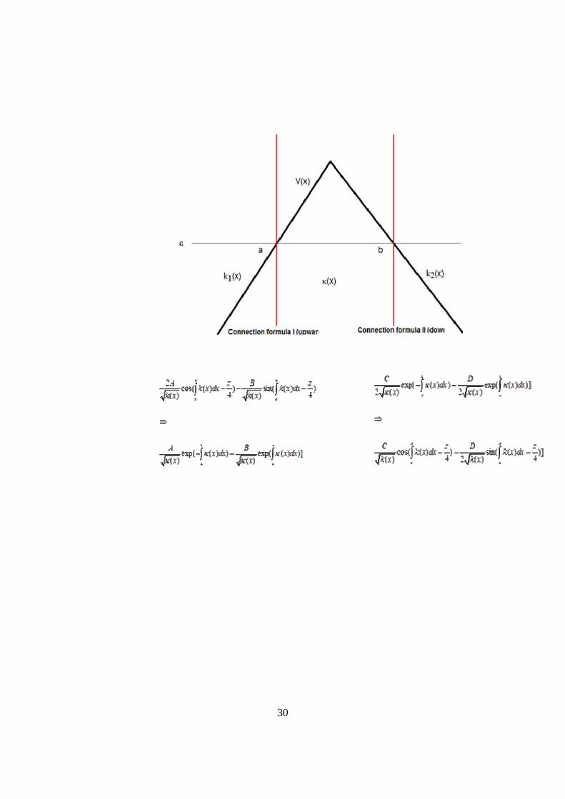
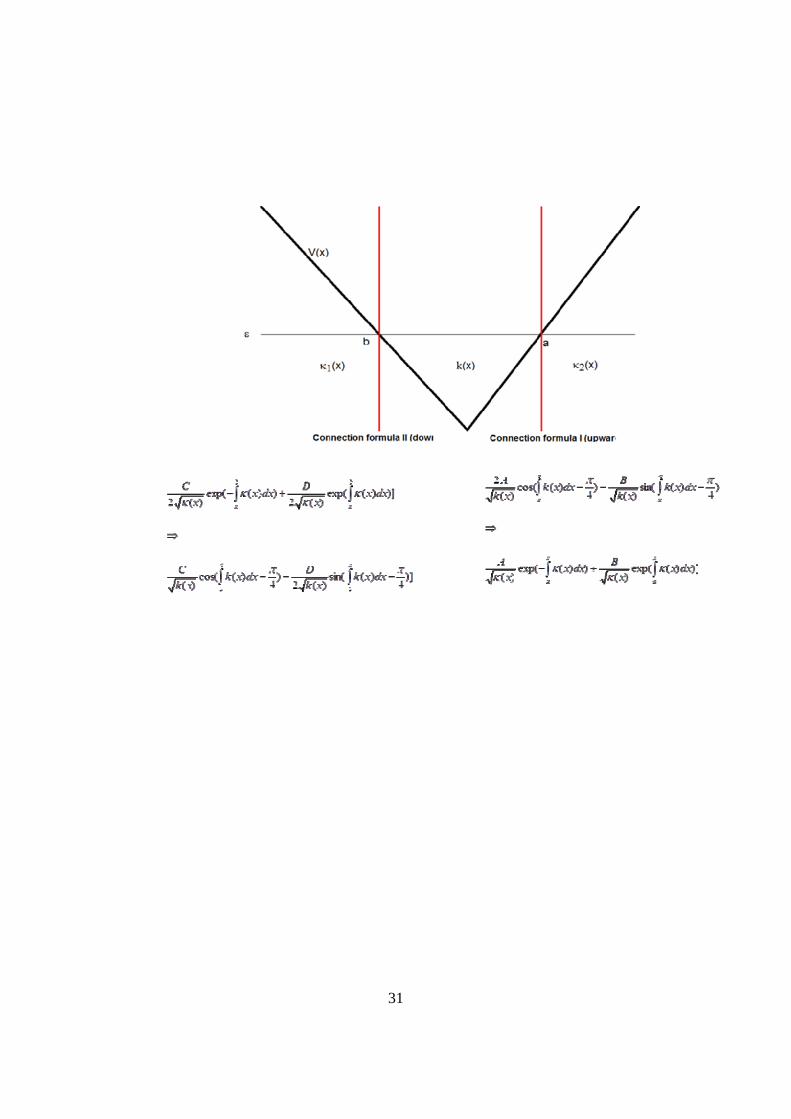
_______________________________________________________________________ APPENDIX Connection formula

)(21

)( xVmxk

)(21

)( xVmx

30

31