Within-Subject Statistical DesignCHAPTER 34- ANALYZING NEURAL TIME SERIES DATA- MIKE X. COHENDANIEL T. GRAYAPRIL 15, 2014

Why perform within-subject statistics?

Evaluate the statistical significance of single-subject results. To test the robustness of an effect in a single subject

Facilitate group-level analysis Transform data to values that are compatible with cross-subject

comparisons (Ie. Normalize the data)

Neural time series data rely heavily on non-parametric permutation testing (Chapter 33)

Basically:

And UNDERSTAND your data before comparing

Goal:

Without within-subject statistical analyses:

Example: Task related power compared to baseline

Before making comparisons between conditions or finding the relationship between neural activity and behavior it is often useful to find specific time-frequency power features which show significant differences. Helps ‘narrow the search,’ and decreases computation time.

Testing power against a null hypothesis of zero is not appropriate since power values cannot be negative (square of the amplitude).

Therefore an appropriate null hypothesis is that there is no change in power relative to a baseline. Note: baseline MUST be within subject.

Testing for changes in power within a subject.

Remember: We are interested in changes from

a baseline, but power law scaling (Chapter 18) does not allow for comparisons across frequency bands using raw values.

Baseline normalize.

Non-parametric permutation testing and pixel or cluster level correction for multiple comparisons.

Ways of permutation testing for changes in time-frequency power relative to a baseline.

Continuous variables

Examples Reaction time

Running speed (rodents)

Pupil diameter

Heart rate

Environmental events

Etc.

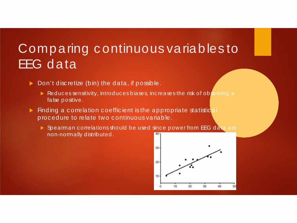
Comparing continuous variables to EEG data

Don’t discretize (bin) the data, if possible. Reduces sensitivity, introduces biases, increases the risk of observing a

false positive.

Finding a correlation coefficient is the appropriate statistical procedure to relate two continuous variable. Spearman correlations should be used since power from EEG data are

non-normally distributed.

The brain consists of many complex interactions, therefore univariatecorrelation can be limiting

In other words:

Variables Interact!

Comparing more than one variable to EEG data

Should perform a multiple regression analysis and not multiple separate correlations. Applying multiple single

correlations can inflate or misrepresent multivariate relationships which leads to a higher likelihood of detecting false alarms.

Multiple Regression

Create a design matrix with as many rows as there are trials and as many columns as there are independent variables.

Fit the matrix to the data using ordinary least squares. The goal is to obtain regression coefficients for each regressor that

express the mapping of the regressor to the data.

Multiple Regression

ß = XYT/XXT

Where ß is the vector of regression coefficients, X is the design matrix, Y is the data matrix, and T indicates the transpose.

Therefore XXT is the covariance of the regressors, and XYT is the variance between the regressorsand the data.

Significance of the ß coefficient is then obtained through non-parametric approaches (for EEG data)

Example 2: Statistical Significance of Phase-Based Data

ITPC or ISPC Several strategies

1: Test the difference in ITPC between conditions or pre and post-trial time.

2: Test ITPC significance on its own (can be approximated using Rayleigh’s Z (Chapter 19).

3: Non-parametric permutation testing

1: Test the difference in ITPC between conditions or pre and post-trial time.

The question here is not whether ITPC is significant, but rather if the ITPC differs between conditions or time segments.

Since ITPC is bound between 0 and 1, their differences will be bound between -1 and 1. Therefore under the null hypothesis the distribution of Z-transform of the ITPC difference will be normal.

Test the difference distribution against this null distribution.

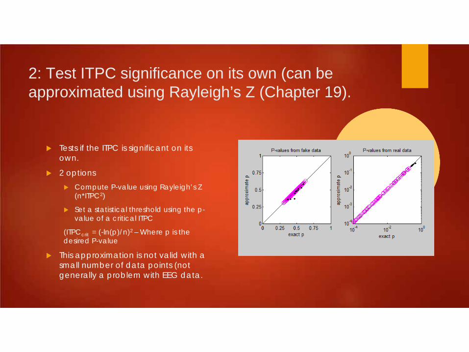
2: Test ITPC significance on its own (can be approximated using Rayleigh’s Z (Chapter 19).

Tests if the ITPC is significant on its own.

2 options Compute P-value using Rayleigh’s Z

(n*ITPC2)

Set a statistical threshold using the p-value of a critical ITPC

(ITPCcrit = (-ln(p)/n)2 – Where p is the desired P-value

This approximation is not valid with a small number of data points (not generally a problem with EEG data.

3: Non-parametric permutation testing for ITPC

Good for exploratory analyses since multiple comparisons are better controlled for than in methods 1 and 2.

ITPC is driven by consistencies in the timing of frequency-band specific activity over many trials. Thus shifting the time course of

phase angles should not effect the final ITPC strength.

NOTE:

These tests evaluate the magnitude of the length of the average ITPC vector, but not the mean phase angle (The phase angle at which maximum clustering occurs is different).

If this is the case use the gv-test (Chapter 26) or phase bifurcation which tests whether phase distributions are different between two conditions.

Assessing significance of correlation coefficients

The easiest way in matlab(according to Mike) is to find the t-statistic, and convert this to a p-value (see Below). T = r((n-2)/(1-r2))1/2

Descent amount of math involved in converting t-statistic to p-value. Luckily, the function tcdf returns a p-value associated with the t-statistic. P-value = tdcf (t,n-2)

Slight exaggeration

Problem

The tcdf function returns the probability of a value being smaller than a t-value, so large negative regression coefficients will give a number close to 0, even though the correlation is strong.

Solution: 1- tdcf(abs(t), n-2)

This ensures that the p-value will approach 0 as the regression coefficient become increasingly strong, whether it be positive or negative.

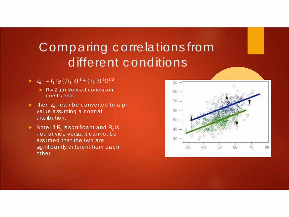
Comparing correlations from different conditions

Zdiff = r1-r2/((n1-3)-1 + (n2-3)-1))1/2

R = Z-transformed correlation coefficients.

Then Zdiff can be converted to a p-value assuming a normal distribution.

Note: if R1 is significant and R2 is not, or vice versa, it cannot be assumed that the two are significantly different from each other.

Remember

Most studies will have more than one subject, so everything presented in this chapter is used to analyze and validate results from a single subject. Some exceptions in non-human

primate studies, but they are rare.

Comparisons will have to be made across subjects.

Hence, we have another presentation today.

Thank you!