Wireless Link Scheduling undera Graded SINR Interference Model

Paolo Santi∗ Ritesh Maheshwari† Giovanni Resta∗ Samir Das† Douglas M. Blough‡

AbstractIn this paper, we revisit the wireless link scheduling prob-lem under a graded version of the SINR interferencemodel. Unlike the traditional thresholded version of theSINR model, the graded SINR model allows use of “im-perfect links”, where communication is still possible, al-though with degraded performance (in terms of data rateor PRR). Throughput benefits when graded SINR modelis used instead of thresholded SINR model to scheduletransmissions have recently been shown in an experimen-tal testbed. Here, we formally define the wireless linkscheduling problem under the graded SINR model, wherewe impose an additional constraint on the minimum qual-ity of the usable links, (expressed as an SNR thresholdβQ). Then, we present an approximation algorithm forthis problem, which is shown to be within a constant fac-tor from optimal. We also present a more practical greedyalgorithm, whose performance bounds are not known, butwhich is shown through simulation to have much betteraverage performance than the approximation algorithm.Furthermore, we investigate, through both simulation andimplementation on an experimental testbed, the tradeoffbetween the minimum link quality thresholdβQ and theresulting network throughput.

1 IntroductionEver since Gupta and Kumar’s classical result [10]

showing that the capacity of multi-hop wireless networksdoes not scale linearly with the number of nodes, re-searchers have studied a multitude of ways to increasethroughput in such networks. Many of the consideredapproaches focus on increasing the concurrency of com-munications in the wireless medium, by separating com-munications either in frequency or in space. Concurrentcommunications can be separated in frequency by usingmultiple channels, with or without multiple radios. A va-riety of techniques exist for improving spatial separation,or spatial reuse, within the wireless channel. These tech-niques apply different methods for reducing or eliminat-ing interference. For example, directional antennas fo-cus the signal in a certain direction, thereby preventing atransmission from interfering with other communicationsoutside of the focused area. Transmission power controlcan reduce the overall “inteference footprint” of a com-munication. More recently, MIMO technology has beenconsidered, both as a means to improve throughput on in-dividual links and for its ability to suppress interference,thereby permitting increased spatial reuse.

∗ Stony Brook University, NY, USA† IIT-CNR, Pisa, Italy‡ Georgia Institute of Technology, Atlanta, GA, USA

Another research focus has been TDMA approachesfor multi-hop wireless networks [14]. TDMA has beenconsidered for its ability both to improve throughputand to provide fairness to flows of differing lengths,which has been shown to be a significant problem inCSMA/CA-based wireless multi-hop networks. TDMAhas been adopted for use in the IEEE 802.16 standard forWiMax [1]. With use of TDMA, comes the opportunityto develop scheduling algorithms that can carefully sepa-rate communications in space, thereby maximizing con-currency and presumably throughput, as well.

When considering the scheduling of transmissions ina multi-hop wireless network, it is necessary to model in-terference. Over time, the research in wireless schedul-ing has considered more accurate interference models.Early work used a simplek-hop interference model, whilelater work employed more accuracte distance-based mod-els. In the last few years, several papers [3, 4, 9] haveconsidered transmission scheduling under more accuratephysical interference models, which are based on signalto interference and noise ratio (SINR) at the receiver.However, all of this recent work has considered thatpackets are successfully received only when SINR ex-ceeds a given threshold, and assumes that packet recep-tion rate (PRR) is zero below this threshold. In reality,PRR falls off gradually with decreasing SINR. This phe-nomenon has been well documented in the literature, andthe SINR region corresponding to imperfect (but consid-erably greater than 0) reception rates is known astran-sitional region, or gray region[15, 16, 23]. In this pa-per, we formulate a graded physical interference model,which accounts for this more accurate relationship be-tween PRR and SINR, and we investigate the question ofwhether scheduling algorithms can effectively use linksthat operate below the SINR threshold in order to increasespatial reuse and thereby improve throughput.

To the best of our knowledge, non-thresholded SINR-based interference models have been seldom used in thewireless scheduling literature, with a few notable excep-tions [7, 8]. However, the emphasis in [7, 8] is on jointlyoptimizing routing, scheduling, and transmit power in or-der to minimize the total average transmit power, givensome constraints on the minimum data rate achieved oneach link. Furthermore, the approach of [7] is based onconvex programming, which has exponential time com-plexity, while that of [8] is based on solving a complexfixed point equation.

In addition to developing a graded SINR model ofpacket reception, we consider the design of scheduling al-gorithms that take advantage of this more accurate model.We present a scheduling algorithm,GradedSINR, and we

prove that this algorithm is within a constant factor ofoptimal in terms of the length of the schedules it pro-duces. We then turn to evaluation of the graded SINRmodel and associated scheduling algorithms in practicalsettings. We present both simulation-based results and anexperimental evaluation carried out using a Mote-basedtestbed. Simulation results demonstrate thatthroughputincreases of up to 50%are possible relative to thresh-olded SINR models. The throughput increase achievedis dependent upon node density, with more improvementseen for sparse networks, where additional opportuni-ties for spatial reuse can have more impact. However,even in dense networks, throughput improvements of al-most 20% were achieved. Results from the Mote-basedtestbed confirm that use of lower-quality links can im-prove throughput. In fact, even greater throughput in-creases, up to 70% improvement over using only 100%quality links, were seen in the testbed. This proof-of-concept implementation also demonstrates the practical-ity of our approach. Thus, we believe that graded SINR-based scheduling algorithms hold great promise for dra-matically improving performance of TDMA-based multi-hop wireless networks.2 The graded SINR model

The graded SINR model is motivated by the observa-tion that, in a practical scenario, the packet reception rate(PRR) vs. SINR is not sharply thresholded, but ratherpresents a smooth transition between close to 0 and closeto 1 reception rate. The region in which packet receptionis not perfect is known as thetransitional region, or grayregion in the literature [15, 16, 23], and typically spans 5to 10 dBs.

In graded SINR models, originally proposed in [15,16], the PRR achievable on a certain link is a function ofthe SINR value experienced at the receiver. The PRR vs.SINR curve has the following properties in these mod-els: i) the PRR is 0 when the SINR is below a certainvalue, which we denoteβ0 in the following; ii) the PRRis 1 when the SINR is above a certain value, which wedenoteβ1 in the following; iii ) the PRR is anincreasingfunction of the SINR in the transitional region. We adoptthis model in this paper, with the further requirement(needed for technical purposes) that limx→β+

0f (x) = 0 and

limx→β−1f (x) = 1, where f () is the function represent-

ing the PRR vs. SINR curve in the[β0,β1] interval. Wealso assume in the following thatβ0 > 0, which is per-fectly reasonable in a realistic scenario (note that SNRand SINR are expressed as linear ratios, not indB). Anexample of such a function whenf is a linear functionis shown in Figure 1. For clarity of presentation, in thefollowing we extend functionf () as follows: f (x) = 0 ifx≤ β0, and f (x) = 1 if x≥ β1.

In the following, we denote a communication link asl i = (si , r i), wheresi is the sender andr i is the receivernode. According to our model, the PRR experiencedon link l i , in the absence of interference,is given byf (SNRi), whereSNRi is the signal-to-noise ratio at noder i . Formally,SNRi = Pi

N , wherePi is the received power atnoder i of the signal transmitted by nodesi , andN is the

PRR (rate)

SINRβ1β0

1

βQ

minimum linkquality requirement

Figure 1. The graded SINR model. Therate is in-tended as normalized w.r.t. maximal possible rateWmax.background noise power.

In presence of multiple concurrent transmissions onlinks l1, . . . , lk, the PRR on linkl i = (si , r i) is givenby f (SINRi), where SINRi is the signal-to-noise-and-interference ratio measured atr i when all thesjs are trans-mitting. Formally,

SINRi =Pi

N+∑ j 6=i Pj,

wherePj denotes the received power at noder i of the sig-nal transmitted by nodesj , for eachj 6= i.

It is worth observing the similarities between thegraded SINR model and the generalized physical interfer-ence model (see, e.g., [13]), according to which thedatarate Wi observed on linkl i is given by Shannon’s channelcapacity formula, i.e.,

Wi = Blog2 (1+SINRi) , (1)

whereB is the channel bandwidth1. The graded SINR in-terference model introduced above can be interpreted interms of data rate as follows. Assume the channel has amaximal nominal data rateWmax. We can interpret thePRR vs. SINR curve as a data rate vs. SINR curve.The idea is that, when the SINR value is below the min-imum thresholdβ1 required for successful transmissionof a packet at rateWmax, PHY layer parameters such ascoding (e.g., increasing bit redundancy in packet trans-mission) and/or symbol sending rate are modified, so thatpackets can be successfully received atr i . Hence, we canview the situation as if packets are always correctly re-ceived when transmitted on linkl i , but with the achieveddata rate depending on the experienced SINR value atr i .Given this interpretation, the main difference between thegraded SINR model and the generalized physical interfer-ence model is that actual data rate on linkl i is 0 under thegraded SINR model whenSINRi ≤ β0, while it is alwaysgreater than 0 with a positive received signal power underthe generalized physical interference model.

Unless otherwise stated, in the following we will usethe data rate interpretation of the graded SINR model,since it eases the derivation of clean approximationbounds for the considered scheduling problem. In orderto keep the values off () in the [0,1] interval, we will in-terpret functionf () as giving, for a certain SINR value,

1Note that the SINR in the formula forWi is expressed as alinear ratio, notdBs.

the resulting data rate normalized with respect to the max-imal nominal data rateWmax. Hence, the actual data rateon link l i with SINR valueSINRi will be f (SINRi) ·Wmax.To simplify notation and when clear from the context, inthe following we will sometimes overload thef (SINRi)notation to denote the data rate on linkl i . Since the datarate interpretation of the graded SINR model assumes ac-curate control of PHY layer parameters is possible, whichis not always the case in practical scenarios, in the experi-mental setup reported in Section 5 we have used the origi-nal, PRR-based interpretation of the graded SINR model.

3 Scheduling Algorithm3.1 Problem Formulation

The problem we consider is often referred to as thewireless link scheduling problemin the literature, al-though we are introducing here an extension to dealwith the case of imperfect link transmissions (or, equiv-alently, flexible data rates). We are given a set of linksL = {l1, . . . , ln} to schedule, withl i = (si , r i). Note thatthe sis andr is are not necessarily distinct, i.e., a singlenode can be involved in multiple communication as ei-ther transmitter, or receiver, or both.

A link l i is assigned a weightdi , which represents thecurrent traffic demand on linkl i . To simplify presentation,in the following we assume unit link demands (i.e.,di = 1for i = 1, . . . ,n). However, the presented results can easilybe extended to the case of arbitrary integer demands byreplacing each linkl i with di copies of the same link.

Links experience different SNRs at the receiver end;i.e., when only transmittersi is transmitting, noder i willexperience a certain SNR valueSNRi , which is in gen-eral different for different receivers. However, in the fol-lowing we assume theSNRi ≥ βQ for eachi, for someconstant valueβQ ≥ β0. Given our model, this is equiva-lent to assuming that data rate (or, equivalently, PRR) oneach link is at leastk, for some constantk > 0 (see Fig-ure 1). The SNR lower boundβQ on the links to sched-ule is introduced to reflect the fact that, in practical situa-tions, only relatively high quality links (i.e., with accept-able data rate, or with a PRR considerably above 0) areused to transmit packets.

The problem we consider is to schedule links in setLin such a way that:i) the demands on each link are satis-fied, andii) the length of the schedule is minimum. Notethat, with respect to classical scheduling problems withnon-graded interference models (e.g., with the physicalinterference model [3, 9]),we do not impose any feasi-bility constraint on the schedule. This is because underthe graded SINR model every transmission set is feasi-ble. What changes is the data rate (equivalently, PRR)experienced on each link, which is dictated by the gradedSINR model, and can actually be 0 on some of the links.Feasibility of the schedule is, in a sense, captured by con-dition i), which states that demands on each link must besatisfied. This implies that, if we define a unit of time asthe time needed to send a unit of demand (packet) fromtransmitter to the intended receiver at rateWmax

2, the total

2Note that this time in practice depends also on the trans-

time allocated for transmission on linkl i in the schedulemust be sufficient to send the packet to destination at theachieved data rate. To be specific, if linkl i is scheduledfor time intervalst1, . . . , th, and the experienced SINR val-ues atr i during these intervals areSINRi,1, . . . ,SINRi,h,we must have∑ j=1,h f (SINRi, j) ·Wmax· t j ≥ S, whereS isthe packet size in bits.

The computational complexity of the link schedul-ing problem has been studied under different interfer-ence models, and has been proven to be NP-hard in manycases, e.g. the physical interference model [9] and mosthop-based interference models [21]. While similaritiesof the graded SINR model with the physical interferencemodel suggest that the problem might remain NP-hardalso in the graded SINR model, a formal proof of this factis beyond the scope of this paper and, to the best of ourknowledge, the problem remains open.

In the following, we present an algorithm for this prob-lem and prove a worst-case bound on its performancewith respect to performance of an optimal scheduling al-gorithm. In order to prove the approximation bound, weadopt the classical model for radio signal propagation inwireless networks, which is referred to as thelog-distancepath loss model. In this model, the radio signal strength(power) at a distanced from the transmitter is given byP/dα, whereP is the transmission power andα > 2 is thepath loss coefficient [19] (the actual value of the constantα depends on the environment – e.g., indoor or outdoor).Our results should be easily extensible to more generalradio propagation models that account for irregular radiocoverage area, such as the cost-based model proposed in[20], which approximates log-normal shadowing propa-gation. In the following, we assume all nodes use thesame transmit power, an arbitrary constantP.3.2 Algorithm GradedSINR

Algorithm GradedSINR, which is reported in Figure2, is based on the simple idea of grouping links with sim-ilar SNR values in the same class, and scheduling themin consecutive slots. Link classes are defined as follows:link classCk, with k = 1, . . . , k, contain linksl js such that

(1+ ε)k−1βQ ≤ SNRj < (1+ ε)kβQ , (2)

where ε is an arbitrary constant≥ 1/7 and k =blog1+ε(P/βQN)c+ 1. Note that: i) all links belong toone of theCks, since the minimum SNR value of links isβQ, and the maximum SNR value isP/N;3 ii) the numberk of link classes is aconstant, i.e., it does not depend onthe numbern of links to schedule.

Note that, under our working assumption of log-distance radio propagation with path loss exponentα > 2,links in thek-th SNR class have length

Dk+1 =(

P(1+ ε)kβQN

) 1α

< Lk≤(

P(1+ ε)k−1βQN

) 1α

= Dk .

mitter/receiver separation. Hence, time unit can be interpretedas themaximumover setL of the time needed to send a packetfrom transmitter to receiver.

3By fundamental laws of physics, the received signal powercan be at most as large as the transmitted power.

Algorithm GradedSINR:

Input: A setL of n links with unit demandOutput: A scheduleS1, . . . , St under graded SINR model

1. t = 12. LetC = {C1, . . . ,Cblog1+ε(P/βN)c=k} be link classes defined as in (2)3. for eachCk 6= /0, with 1≤ k≤ k4. Partition network deployment region into squares

of width µk ·Dk+15. 4-color the squares such that no two adjacent squares

have the same color6. for j = 1, . . . ,47. Select colorj8. repeat9. For each squareA of color j, choose a linkl i ∈Ck

with receiver inA; Lkj = Lk

j ∪{l i}10. t = t +1; St = Lk

j

11. set duration of slotSt to 1/ f ((1+ ε)k−2βQ)12. until all links of Ck in selected squares are scheduled13.return S1, . . . , St

Figure 2. TheGradedSINRAlgorithm.When considering links in class 1≤ k≤ k, the deploy-

ment region is divided into square cells of sideµkDk+1,where constantµk is defined as follows:

µ= 2

(64(1+ ε)k−1βQ(α−1)

α−2

) 1α

.

Cells in the same class are then 4-colored in such away that no two adjacent cells have the same color. Then,at Steps 6–12 links are greedily scheduled in successiveslots, with the property that only links with the same colorwhose receivers are in different cells are assigned to thesame slot.

At Step 11, the duration of slots whose links are inclassk is set to 1/ f ((1+ ε)k−2βQ), which, as shown inthe following, is sufficient to send a unit of demand alongthe scheduled links. In fact, cell dimensioning is suchthat, under the hypothesis fulfilled byGradedSINRthatno two links with receivers in the same cell of colorj arescheduled concurrently, the minimum SINR value at eachscheduled receiver is at least(1+ ε)k−2βQ.

We now formally prove that the schedule computed byGradedSINRsatisfies the traffic demands of all links inL.THEOREM 1. Assume that17 ≤ ε ≤ 63 and βQ ≥ 1.Then, the schedule computed by Algorithm GradedSINRsatisfies the traffic demands of all links in L.PROOF. Let us consider a slot containing links in classCk, for some 1≤ k ≤ k. We now upper bound the in-terference experienced by a receiverr in a certain cellC in the partitioning obtained for classCk. Once wefocus on a receiverr i in specific cellC , the cells con-taining receivers of the interfering links can be arrangedin circumcentric square frames aroundC . The innerframe contains 32−12 = 8 cells, the second frame con-tains 52− 32 = 16 cells, and in general theh-th framewill contain (2h + 1)2 − (2h− 1)2 = 8 · h cells. Thegeneric receiver contained in theh-th frame will be atleast(2h− 1)µkDk+1 apart fromr i . Considering that inclassk all links have a length smaller thatDk, the mini-mum distance betweenr i and asenderrelative to framehis (2h−1)µkDk+1−Dk =(2h−1)µkDk/(1+ε)1/α−Dk =

Dk((2h−1)µk(1+ ε)−1/α−1). Hence, the total interfer-enceIr experienced byr i can be upper bounded by

Ir <∞

∑h=1

8h·PDα

k · ((2h−1)µk(1+ ε)−1/α−1)α (3)

≤ 8PDα

k

∞

∑h=1

h

(12(2h−1)µk(1+ ε)−1/α)α

(4)

=8(1+ ε)P

(1/2)αµαk Dα

k

∞

∑h=1

h(2h−1)α (5)

≤ 8(1+ ε)P(1/2)αµα

k Dαk

∞

∑h=1

h(2h−h)α (6)

=8(1+ ε)P

(1/2)αµαk Dα

k

∞

∑h=1

1hα−1 (7)

≤ 8(1+ ε)P(1/2)αµα

k Dαk· α−1

α−2(8)

where (4) follows becausex−1 > x/2 for x > 2 and in-deed(2h−1)µk(1+ε)−1/α is greater than 2 under the the-orem assumptions, and (8) follows from a known boundon Riemann’s zeta function.The SINR for the receiverr i can thus be bounded by

SINRi ≥P

Dαk

Ir +N≥

PDα

k

8(1+ε)P(1/2)αµα

k Dαk· α−1

α−2 +N=

=P

Dαk

P8(1+ε)k−2βQDα

k+N

=(1+ ε)k−1βQN(1+ε)k−1βQN8(1+ε)k−2βQ

+N=

=(1+ ε)k−1βQ

(1+ε)8 +1

=8· (1+ ε)(1+ ε)+8

· (1+ ε)k−2βQ ≥

≥ (1+ ε)k−2βQ , (9)

where (9) follows sinceε ≥ 17.

Since linkl i in classCk, for some 1≤ k≤ k, is sched-uled in a slot of duration 1/ f ((1 + ε)k−2βQ), and the(normalized w.r.t. Wmax) data rate on linkl i is at leastf ((1+ ε)k−2βQ) (recall thatf () is an increasing functionof SINR), we have that at least one unit of demand can betransmitted on linkl i in the scheduled slot, and the theo-rem follows.DEFINITION 1. Given a set L of links to schedule, theSNR densityfor link class Ck, with 1≤ k≤ k, is the max-imal number of receivers in a cell of class Ck, and is de-noted∆k.DEFINITION 2. Given a set L of links to schedule, thenormalized SNR densityfor L, denotedΨ(L), is definedas

Ψ(L) = max1≤k≤k

{∆k

f ((1+ ε)k−2βQ)

}.

We now prove an upper bound on the length of theschedule computed by AlgorithmGradedSINR.THEOREM 2. The schedule computed by AlgorithmGradedSINR has O(Ψ(L)) length.

PROOF. Links in classCk, for 1≤ k≤ k, whose receiversare in a cell of color, say,j, are scheduled in parallelif they are in different cells; hence, the number of slotsneeded to accommodate all links in classCk is the num-ber of colors (four) times the number of receivers in themaximally occupied cell, i.e.,∆k. Since slot duration forlinks in classk is 1/ f ((1+ε)k−2βQ), total schedule length

is upper bounded by∑kk=14· ∆k

f ((1+ε)k−2βQ) ≤ 4· k ·Ψ(L) ∈O(Ψ(L)) sincek is a constant.

We are now ready to prove the approximation boundfor Algorithm GradedSINR.THEOREM 3. Algorithm GradedSINR computes aschedule whose length is within a factor O(1) fromoptimal.PROOF. Let us consider a link classCk for which thenormalized SNR densityΨ(L) is achieved, and letLk =l1, . . . , l∆k

be links in classCk whose receivers are in amaximally occupied cell. Call this cell thecritical cell.We lower bound the time needed to schedule links inLkonly. Clearly, since the optimal schedule must accom-modate a possibly larger set of links, the computed lowerbound applies also to the optimal schedule for link setL.We start by proving an upper bound on the number of fea-sible transmissions with receivers belonging to the criti-cal cell, under the assumption that the feasible rate on thelinks is at leastf (β), for some 0< β0 < β < (1+ ε)kβQ.Note thatβ must be greater thanβ0 in order to have a non-zero data rate on the link, and that the maximum data rateof links in classCk is < (1+ ε)kβQ. In particular, weprove that no more than

qk,β = ((1+ ε)1/α +√

2µk)α · (1+ ε)kβQ−β

β(1+ ε)kβQ

such transmissions can occur in parallel. The value ofqk,βis obtained by solving the following inequality

P(Dk+1)α

N+x · P(√

2µkDk+1+Dk)α

=(1+ ε)kβQN

N+x · (1+ε)kβQN

(√

2µk+(1+ε)1/α)α

< β

(10)which, after straightforward algebraic manipulation,leads to

x < ((1+ ε)1/α +√

2µk)α · (1+ ε)kβQ−β

β(1+ ε)kβQ

from which the above value ofqk,β is obtained. Inequality(10) comes from assuming the largest possible receivedpower at the numerator, and the minimum possible con-tribution to interference from links whose receiver end isin the critical cell.Let us consider the schedule computed by the optimalalgorithm, and letx > 0 be the minimum data rate of alink in the optimal solution. Defineβ as the SINR valuecorresponding to data ratex according to functionf (),i.e., f (β) = x. Given the previous result, we have that atmostqk,β links, each with rate≥ x, can be scheduled inparallel. The data rate on each of these links is at most

0 time

l 1

l 2

l 3

l 4

S1 S2 S3 S4 S5 S6 S7 S8 S9

Figure 3. Example of possible link schedule under thegraded SINR model. The data rate on, e.g., linkl1is different in slot S1,S2,S3,S4,S6,S7,S8 in which it isactivated.f ((1+ ε)kβQ), since all the links in the critical cell be-longs to classCk. Since valuesqk,β are adecreasingfunc-tion of β, we have that the maximum demand that canbe satisfied in a unit of time in the optimal schedule isqk,β · f ((1+ ε)kβQ). Since the total demand of links inthe critical cell is∆k, we have that the length of the opti-mal schedule is at least

∆k

qk,β · f ((1+ ε)kβQ).

We now have that the ratio between the schedulelength of the optimal solution and that of the schedulecomputed byGradedSINRis

O

(Ψ(L) ·qk,β · f ((1+ ε)kβQ)

∆k

)=

= O

(∆k

∆k·qk,β · f ((1+ ε)kβQ)

f ((1+ ε)k−2βQ)

)= O(1)

since functionf (x) has values in the interval(0,1] whenx > β0, and(1+ ε)k−2βQ > β0. This concludes the proofof the theorem.

Note the importance of the result stated in Theorem3: under the graded SINR model, different transmissionsets can be active at different times, possibly using flex-ible slots of very different time duration (see Figure 3).Hence, finding the optimal schedule in such a large set ofpossible solutions appears to be a very difficult task (al-though not yet formally proved to be NP-hard). Theorem3 states that by imposing a strict structure on the schedule(all links of the same SNR class are scheduled in con-tiguous slots of fixed duration), we can still obtain a solu-tion which is close to optimal (in asymptotic sense). Thisis especially important since, while general schedules al-lowed under the graded SINR model as the one depictedin Figure 3 can be difficult to realize in a practical setting(due to, e.g., required PHY layer parameter tuning whilea packet is in the air), the well structured schedule com-puted byGradedSINRcan be implemented more easilyin a practical setting.

4 Simulation-based evaluationIn this section we extensively evaluate the perfor-

mance of scheduling algorithms based on the gradedSINR model through simulation. The main goals of theevaluation are: (1) to identify the throughput maximizing

configuration of the link quality thresholdβQ under dif-ferent node density and topology/radio propagation sce-narios, and (2) to quantify the potential throughput ad-vantages of using the graded SINR model compared to astrict threshold-based SINR model. In view of (1), the in-teraction between scheduling and routing has to be con-sidered: in fact, as the link quality threshold is varied,different sets of links are made available to the routingprotocol and possibly used to route messages to the des-tinations. Hence, what specific routing protocol is used isan important choice that eventually determines the trafficload experienced on the available links.

In general, maximum throughput can be obtained onlyby jointly optimizing routing and scheduling, possiblyexploiting multi-path routes (see, e.g., [2, 6]). How-ever, joint routing and scheduling optimization under thegraded SINR model is an open problem that is beyond thescope of this paper. Here, we are concerned with optimiz-ing the scheduling step after a certain routing algorithmhas been executed, and link demands generated. Hence,in our simulations, we will consider a simple (yet signif-icant) routing algorithm coupled with a traffic generationmethod tailored to a wireless mesh network scenario, anduse these two components to generate the link traffic de-mands given as input to the various scheduling algorithmsconsidered.

4.1 Simulation setupThe simulation setup is tailored to a wireless mesh net-

work scenario. A set ofn nodes is deployed in a square re-gion of sideL. Two deployment methods are considered:grid-like, and uniform random. After node deployment,then×n link matrix M is generated, where entrymi, j ofthe matrix represents the channel gain between transmit-ter nodei and receiver nodej. Channel gains are com-puted based on node positions, and on the radio propaga-tion model. Radio signal propagation obeys log-normalshadowing, with path loss exponentα, for someα > 2,and varianceσ.4 After the channel matrix is generated,a fixed fraction of the nodes (0.1) is selected as gatewaynodes, according to a uniform random distribution. Foreach non-gateway node, a traffic demand is generated byrandomly and uniformly choosing an integer in the inter-val [1,5]. The generated traffic is directed to gateways, ac-cording to the following routing scheme. First, anavail-able link matrix AMis obtained fromM by retaining en-triesmi, j such that the SNR value at the receiver nodej isat leastβQ, whereβQ is the desired link quality threshold.The other entries in matrixAM are set to 0, in order to pre-vent the routing algorithm from using the correspondinglinks. Using matrixAM, the routing algorithm then buildsshortest path trees rooted at the gateway nodes to set upthe routing paths. In case of ties, the gateway to which aspecific node sends its traffic is selected uniformly at ran-dom. The link demands, which constitute the input to thescheduling algorithms, are then computed based on thenode traffic demands and the chosen shortest path trees.

4We have repeated the simulations with log-distance pathloss propagation, obtaining similar results.

The metric used to build the shortest path trees is hop-count. Although very simple, this metric is used by mostof the current routing algorithms for wireless multi-hopnetworks (e.g., DSR [12] and AODV [18]). Furthermore,when coupled with a link quality criterion, using minimalhop routes tends to reduce the total demand on the links,while only marginally sacrificing link throughput (if thelink quality threshold is relatively high). For this reason,we believe shortest path routing based on hop-count is areasonable heuristic to achieve a relatively high networkthroughput.

When using the graded SINR model, functionf () dic-tating the SINR (indB) vs. link data rate relationship isdefined as follows:f (x) = 0 if x≤ β0 = 10dB, f (x) = 1 ifx≥ β1 = 25dB, and f () linearly varies between these twovalues forβ0 ≤ x≤ β1. This setting is coherent with theSINR vs. PRR measurements for WLAN environmentsreported in [16], as well as with Shannon’s capacity for-mula for intermediate SINR values5. We recall that thedata rates returned by functionf () are normalized withrespect to the maximum nominal bit rate of the link, setto 55Mbs in our experiments.4.2 Simulated scheduling algorithms

In addition to AlgorithmGradedSINR, we have alsoimplemented AlgorithmI-GradedSINR, which is an op-timized version ofGradedSINR, as well as a greedy al-gorithm calledGreedyGraded. We do not give details ofGradedSINRdue to length limitations.GreedyGradedisinspired by the algorithm used in [16] to evaluate through-put in the WLAN experimental testbed. More specifi-cally, GreedyGradedorders links randomly, and consid-ers them sequentially. When a specific linkl has to bescheduled, the currently formed slots are scanned, and,for each of them, the duration of the slot if linkl wereto be added is computed. Similarly toI-GradedSINR, theduration of a slot is set to the minimum value needed totransmit a packet along all active links and, hence, is de-termined by the SINR value of the weakest active link.Note then that the duration of the slot ifl were to beadded is in general longer than that of the original slot,since addingl to the slot would degrade SINR values(and, consequently, data rates) at the receiver nodes. LetS(l) be the currently formed slot such that addingl to theslot increases slot duration of the minimal amount of timeT(l). The value ofT(l) is compared with 1/ f (SNR(l)),i.e., the duration of a slot in which only linkl is active.If T(l) < 1/ f (SNR(l)), then link l is added to slotS(l),otherwise a new slot is formed at the end of the schedulewith only link l active. This process is repeated until alllinks have been scheduled.

In order to understand the relative benefits of thegraded SINR model vs. the commonly used, thresh-olded version of the model, we have also implementedthe GreedyPhysicalalgorithm of [3], which is a simplegreedy algorithm that schedules a link in the first availableslot(s), subject to the condition that the resulting transmis-

5We recall that a logarithmic SINR vs. data rate relationshipin the linear scale as in equation (1) is equivalent to a linearrelationship indBscale.

!"#$

!"%$

&$

&"&$

&"'$

&"($

&")$

&"*$

!"*$ !"**$ !"+$ !"+*$ !",$ !",*$ !"#$ !"#*$ !"%$ !"%*$ &$

!"#$%&'($)*+#',-./01$-$)+'

-,)&'(,)2'345(,+6'

7"#$%4($'8$)*+#'1!&'8,)2'345(,+6'9':/,%';<=-'9'80*>0/-'

-./010$

23-./010$

-.1104$

-.1104564$

!"

!#$"

!#%"

!#&"

!#'"

$"

$#$"

$#%"

$#&"

$#'"

("

)#*" )#**" )#&" )#&*" )#+" )#+*" )#'" )#'*" )#," )#,*" !"

!"#$%&'($)*+#',-./01$-$)+'

-,)&'(,)2'345(,+6'

7"#$%4($'8$)*+#'1!&'8,)2'345(,+6'9':/,%';<<-'9'80*=0/-5('

-./010"

23-./010"

-.1104"

-.1104564"

Figure 4. Schedule length improvement for increasing link quality threshold in the dense (left) and sparse (right)grid-like deployment scenario.

!"#$

!"%$

&$

&"&$

&"'$

&"($

&")$

&"*$

&"+$

!"*$ !"**$ !"+$ !"+*$ !",$ !",*$ !"#$ !"#*$ !"%$ !"%*$ &$

!"#$%&'($)*+#',-./01$-$)+'

-,)&'(,)2'345(,+6'

7"#$%4($'8$)*+#'1!&'8,)2'345(,+6'9':5)%';<=>-'9'80*?0/-'

-./010$

23-./010$

-.1104$

-.1104564$

!"

!#$"

!#%"

!#&"

!#'"

$"

$#$"

$#%"

$#&"

$#'"

("

)#*" )#**" )#&" )#&*" )#+" )#+*" )#'" )#'*" )#," )#,*" !"

!"#$

%&'()*+,-*&-*!./)&

$0!%&-0!1&2,3-0/4&

5()*+,-*&6*!./)&7'%&60!1&2,3-0/4&8&93!+&:;<<$&8&6".="#$3-&

-./010"

23-./010"

-.1104"

-.1104564"

Figure 5. Schedule length improvement for increasing link quality threshold in the dense (left) and sparse (right)random deployment scenario.sion set is feasible under the thresholded SINR model.We recall that relative benefits of graded vs. thresh-olded SINR model have been recently quantified in about30% throughput improvements in an experimental testbed[15], although these improvements refer to a different butrelated scheduling problem (single slot scheduling, alsoreferred to as one-shot scheduling).

4.3 Simulation resultsIn a first set of simulations, we distributedn = 100

nodes in a grid-like fashion. Two grid steps are consid-ered, to mimic relatively dense and relatively sparse net-work deployments. Considering that PHY layer parame-ters are set as follows: path loss exponentα = 3, trans-mit power 100mW(20dBm), and noise power−90dBm,we have a resulting nominal transmission range (in ab-sence of shadowing and interference) of about 680m toobtain the maximum data rate of 55Mbs (which, we re-call, requires a SINR≥ 25dB). Hence, we set the gridstep in the dense deployment to 150m, and to 500m in thesparse deployment. In both cases, internode separation israndomly perturbed by up to 10% to avoid artificial dis-cretization effects. The shadowing parameterσ is set to4dB.

In both deployments, 10 nodes are randomly chosenas gateways, and node traffic, routing, and link demandsgeneration is performed as described in the previous sec-tions. The schedule lengths computed byGradedSINR,I-GradedSINR, andGreedyGradedfor a given link qual-ity thresholdβQ are returned as the simulation result6.The simulator returns also the schedule computed byGreedyPhysical, which is based on the thresholded SINR

6Parameterε in algorithmsGradedSINRandI-GradedSINRis set to 1/2.

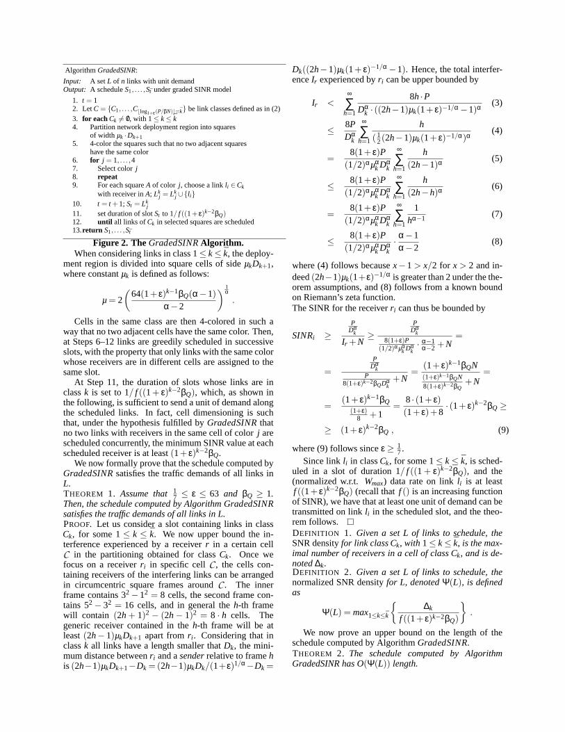
model, and hence invariant to changes in the link qualitythresholdβQ. We have generated 1000 different deploy-ments for both the dense and the sparse scenarios, andconsidered link quality thresholds corresponding to linkdata rates ranging from 50% to 100% of the maximumnominal rate. Simulation results are shown in Figure 4.

We have also considered a random node deploymentscenario, in which nodes are distributed uniformly at ran-dom in a certain square region. Similarly to the case ofgrid-like deployment, we have set the side of the deploy-ment area to relatively small (1350m) and relatively large(4500m) values, to mimic relatively dense and relativelysparse deployments. In case of sparse deployments, wecheck that each non-gateway node has a path composedof only 100% quality links to at least one gateway node,so that demands can be fully satisfied under the thresh-olded SINR model. Any deployments not meeting thiscriterion are discarded. The results of this second set ofsimulations, also averaged over 1000 experiments, are re-ported in Figure 5.

The plots reported in Figures 4 and 5 report theaverage throughput length improvement of the variousscheduling algorithms, which is normalized with respectto the schedule length of the sequential schedule whenonly 100% quality links are used. As seen from the fig-ures, the trends for the grid-like and random scenariosare similar. In all cases,GreedyGradedwas by far thebest scheduling algorithm, achieving as high as a nearthree-fold throughput improvement with respect to thesequential schedule7. The other scheduling algorithmsfor the graded model, for which, we recall, we have

7In the rest of this section, throughput improvements are al-ways considered to be with respect to the sequential scheduleusing only 100% quality links.

!"

#!"

$!!"

$#!"

%!!"

%#!"

&!!"

&#!"

'!!"

'#!"

#!!"

!(#" !(##" !()" !()#" !(*" !(*#" !(+" !(+#" !(," !(,#" $"

!"!#$%&'(#)&%

(*)+%$*),%-.#$*!/%

0"!#$%1'(#)&%23+%4*),%-.#$*!/%5%67*&%

-./0"$#!"

-./0"#!!"

!"

#!"

$!!"

$#!"

%!!"

%#!"

&!!"

&#!"

'!!"

'#!"

#!!"

!(#" !(##" !()" !()#" !(*" !(*#" !(+" !(+#" !(," !(,#" $"

!"!#$%&'(#)&%

(*)+%$*),%-.#$*!/%

0"!#$%1'(#)&%23+%4*),%-.#$*!/%5%6#)&%

-./0"$&#!"

-./0"'#!!"

Figure 6. Total link traffic demand in the grid-like (left) and random (right) deployment scenario.provable performance guarantees with respect to optimal,achieve only marginal throughput improvements (below1.4), withI-GradedSINRconsistently performing slightlybetter thanGradedSINR. Note that, due to the large sizeof the cell partitioning used inGradedSINR, the sched-ule computed by this algorithm always coincided withthe sequential schedule; i.e., due to the very conserva-tive choice of the cell size driven by worst-case consid-erations,GradedSINRwas unable to achieve any spatialreuse. This lack of spatial reuse, coupled with possibleusage of lower quality links (hence, longer slots) whenthe lower bound on link quality is below 100%, and withthe fact that the total demand does not depend on the linkquality threshold in dense deployments (see Figure 6), ex-plains the relative throughputdegradationwith respect tothe sequential schedule with 100% quality links experi-enced byGradedSINRin dense deployments when usingweak links is allowed.

When comparing the dense and sparse scenarios, weobserve higher throughput improvements in the sparsescenario: close to three-fold improvements are achievedin the sparse deployments, compared to no more than 1.5-fold improvements in the dense setting. This difference isdue to the additional opportunities for spatial reuse in alarger, i.e. sparser, network deployment.

Concerning the impact of link quality threshold onschedule length, we observe a clear effect of node den-sity for the more aggressive scheduling algorithm, namelyGreedyGraded: when the network is dense, the sched-ule length tends to increase as the lower bound on linkquality decreases, implying that allowing use of relativelyweak links is detrimental for network throughput. Tothe contrary, in sparse network deployments, using rel-atively weak links can improve throughput: about 10%(5%) further improvements are observed when the linkquality threshold is reduced from 100% to 80% (85%)in the grid-like (random) case. In both cases, further re-ducing the link quality threshold has negative effects onthroughput.

The radically different behavior in case of dense orsparse networks can be explained by the data reported inFigure 6, which shows the total traffic demand as a func-tion of the link quality threshold. In case of dense de-ployments, the total demand does not depend on the linkquality threshold, indicating that, even for the most strin-gent link quality requirement, relatively short paths to thegateways are available. The throughput degradation thatis observed in case of lower link quality thresholds is due

to the fact that the routing algorithm is oblivious to linkquality when building the shortest path tree; hence, if rel-atively weak links are included in the tree, the average slotduration is increased (lower link rates) which, coupledwith the unchanged total demand, results in an overallthroughput degradation. On the other hand, in sparse net-work deployments total traffic demand considerably in-creases as the link quality threshold increases, indicatingthe short paths to the gateways can be found only if rela-tively weak links are used. Although usage of weak linkstends to increase average slot duration, the lower total de-mand compensates this increase with a reduction in thetotal number of slots, resulting in an overall throughputincrease. However, if very weak links (≤ 75%) are used,the reduction in total traffic demand is no longer sufficientto compensate for the increased average slot duration, re-sulting in an overall throughout degradation.

Finally, we comment on the relative throughput bene-fits of using the graded vs. thresholded SINR interferencemodel: with similar greedy approaches to schedule links,we observe a throughput improvement ofGreedyGradedover GreedyPhysicalof about 18% for dense deploy-ments, and about 50% for sparse deployments. This istrue, even though we are using a routing algorithm thatis oblivious to link quality (except in a relatively crudeway, through use of the link quality threshold). Hence,we expect even larger throughput improvements can beattained when using a link-quality-aware routing algo-rithm. Study of this aspect is left for future work. Nev-ertheless, throughput improvements of up to 50%, evenwith the simple routing algorithm used herein, show thatvery substantial benefits can be achieved through use ofthe graded SINR model.

5 Experimental evaluationThe main purpose of the experimental evaluation is

to study how the choice of link quality threshold affectsthroughput in a real network. We use TelosB motes [17]that are equipped with CC2420 radio [5]. The radio iscompliant with the IEEE 802.15.4 [11] PHY layer stan-dard in the 2.4 GHz ISM band and operates at a fixednominal bit rate of 250 Kbits/s. We have implementeda simple TDMA protocol in TinyOS-2.0 [22] in whichmotes transmit at designated time instants without per-forming carrier sensing or backoff as in the default MACimplementation in TinyOS.

The data rate is fixed due to the choice of hardware.For simplicity, we also fix the transmission power to

−32.5 dBm uniformly on all nodes. Hence, in this sec-tion we use the PRR interpretation of the graded SINRinterference model. Furthermore, we focus our attentionon the simpler and more practical (as well as best per-forming on the average) greedy approach for transmissionscheduling.

The setup of the experimental testbed is similar tothe one used in simulations. More specifically, we de-ploy n = 20 nodes, placed randomly on a 10 foot by 3foot tabletop in an office environment. Through exten-sive measurements we derive the input parameters to the“routing/scheduling” module, which are the following: 1)the n×n channel gain matrixCG, reporting the channelgain between each possible node pair; 2) then×1 noisevector NV, reporting the noise level at each node; and3) the PRR vs. SINR functionf (). The measurementmethodology used to collect 1)–3) is similar to the oneused in [15]. The PRR vs SINR function we obtained issimilar to the one presented in [15]. The function has agraded region from -3 to +5 dB. Beyond a SINR of 5 dB,links always have PRR close to 100%.

The input parameters are fed to a centralized node (aPC) which runs the “routing/scheduling” module as fol-lows. Similarly to the simulation-based evaluation, twoof the nodes are randomly selected as gateways. Non-gateway nodes are assigned an integer demand chosen atrandom in the interval[1,5]. Then, given the link qualitythresholdSNRQ and matrixCG, the set of available linksis determined, and shortest path trees routed at the gate-way nodes are built. Given node demands and the set ofroutes, link demands are computed, which are fed to thescheduling algorithm.

Given the PRR interpretation of the graded SINR in-terference model, a re-design of the link scheduling al-gorithm is needed. In particular, variable slot durationis no longer needed, since link data rate is fixed andthe same for all links. However, a packet scheduled fortransmission along linkl in slot S under the PRR in-terpretation is received only with probabilitypl ,S, with0≤ pl ,S = PRRl ,S≤ 1, wherePRRl ,S is the PRR on linklin slot S. Packet transmissions in a specific slot can thenbe interpreted as Bernoulli trials with a certain, fixed suc-cess probability8. If the schedule is repeatedN times, bythe LLN we have that the expected number of successfultransmissions along linkl in slotSconverges toN · pl ,S asN grows larger. Hence, the expected long-term effectivedata rate on linkl in slot S is pl ,S. Based on this obser-vation, the greedy scheduling algorithm described belowconsiders that an amount of demand equal topl ,S is satis-fied when linkl is scheduled for transmission in slotS.

The scheduling algorithm is as follows. The approachis again greedy: links are initially ordered, and are pro-cessed sequentially. The algorithm keeps extracting ele-ments from the list of links to be scheduled, till the de-mand on all links is satisfied. The main difference withGreedyGradedis that a single link might be consideredrepeatedly when building the schedule (see below).

8This holds true only under the assumption that the radioenvironment is relatively stable.

Figure 7. Normalized aggregate throughput at thegateway nodes as a function of the link quality thresh-old.

When link l is considered, the algorithm sequentiallyscans all currently built slots. For each slotS, the algo-rithm first checks whether addingl to the slot would keepit “feasible” (this is a soft notion of feasibility, describedbelow); if the slot remain “feasible”, the algorithm com-putes a “fitness” measure, namely the difference betweenthe increase in expected throughput due to adding the newlink, and the throughput decreases on the already sched-uled links. The throughput of a slotSis the sum of allpl ,Svalues on the scheduled links. If the “fitness” of the slotis positive (i.e., we have a throughput increase by addingl to the slot), then the slot is a candidate slot for linkl .After scanning all currently available slots, the algorithmaddsl to the slotS with best positive fitnessf it (S). Iff it (S) < 0, a new slot is created at the end of the sched-ule, and linkl only is put in the new slot.

Once link l has been included in a slot, link demandsare updated as follows.Case1. Link l is added to an existing slotS: the demandof l is decreased ofpl ,S; furthermore, the demands of alllinks in S\ {L} is increasedof (pl ,S\{L}− pl ,S). This isto possibly account for PRR degradation of links inS\{L} due to addingl to the slot. Note that if the demandon some of these links were 0 (link already successfullyscheduled), a new instance of the link with the remainingdemand has to be included again in the list of links to bescheduled.Case2. Link l is added to a new slotS′: the demand ofl isdecreased ofpl ,S′ = PRR(l), since only linkl is scheduledin S′.

The soft notion of “feasibility” used in the algorithmis an optimization aimed at ensuring that the demand ona link is decreased of a significant amount when sched-uled in a slot. In particular, we define a set of trans-missionsl1, . . . , lk to befeasibleif pl i ,{l1,...,lk} ≥ PRRq foreachi, wherePRRq < PRRQ is a PRR quality threshold(e.g., 0.5). Note that this threshold is different (and lower)than the quality threshold used to define which links are“good” and usable by a routing algorithm. In fact, the lat-ter threshold refers to the link quality based on the SNR,while the formed on the link quality based on the (lower)SINR value when all scheduled links are simultaneouslytransmitting.

5.1 Experimental ResultsDifferent schedules are obtained by choosing different

link quality thresholds. Once the schedule is computed,it is fetched to the testbed nodes, which repeatedly exe-cute the schedule and transmit packets. Each schedule isrepeated 100 times. The outcome of an experiment is theaggregate throughput measured at the two gateway nodes.Note that, sometimes links can be over-scheduled. Thismeans that the sum of PRRs of a link scheduled in dif-ferent slots might exceed the weight on that link. Thus,as a result, the number of packets successfully received atthe gateways might exceed the number of packetssched-uled to be received. We do not consider these extraneouspackets in our calculation of the throughput.

We present the results of our testbed experiments inFigure 7. The X-axis enumerates the various schedulesgenerated with different link quality thresholds. The linkquality thresholds are varied from SNR values of 1 dB toupto 7 dB. On Y-axis we plot the throughput in terms ofpackets successfully received at the gateways normalizedwith the schedule length, or as packets per slot. As canbe seen, using a lower link quality threshold – even in thetransition region – results in improving the throughput.Infact, 70% better throughput is obtained by using weaklinks (a link quality threshold of 1 dB) compared to verystrong links (7 dB). We conjecture that this is because,by letting the routing protocol utilize weak links, a packetends up taking fewer number of hops to the gateways –thus making the schedule more compact. Lowering linkthreshold further does not give any performance benefitin our testbed giving same results as for the threshold of1 dB. These results show that theGreedyGradedalgo-rithm works quite well in a realmeshnetwork scenario,where packets are routed towards gateways, giving highend-to-end throughput even with relatively weak links.

6 Conclusions and future workWe believe this paper delivers several contributions,

and opens numerous avenues for further research. Fromthe methodological point of view, the paper encompassesall stages of the “from ideas to testbed implementation”process: 1) starting from the formalization of a new inter-ference model and related problem definition; 2) contin-uing with presentation of algorithms with proven approx-imation bounds for the problem considered; then 3) eval-uating performance through simulation, as well as pre-senting a more practical variation of the scheduling algo-rithm; and finally 4) implementing the practical versionof the scheduling algorithm in an experimental testbed,and evaluating its performance in a practical setting.

Several questions are left open by this paper, whichcan be considered only as a starting point towards a bet-ter understanding of the possible benefits of allowing useof “imperfect” links on the resulting network throughput.In particular, the problem of routing and scheduling forthroughput optimization under the graded SINR modelshould be considered. Furthermore, a better understand-ing of the impact of node density on routing/schedulingperformance is needed. From the experimental view-point, an assessment of whether the throughput measured

at the gateway nodes is not only increased, but also pro-portional to actual node demands is needed. Such an as-sessment would make our proposed scheduling approacha promising candidate as a building block for provid-ing strong QoS guarantees in a wireless multi-hop net-work. Finally, implementing the proposed schedulingtechniques with a high data rate technology (e.g., WiFi)is another challenge to be undertaken.

7 References[1] http://ieee802.org/16/[2] M. Alicherry, R. Bathia, L. Li, “Joint Channel Assignment and

Routing for Throughput Optimization in Multi-Radio WirelessMesh Networks”,Proc. ACM Mobicom, pp. 58–72, 2005.

[3] G. Brar, D. Blough, and P. Santi, “Computationally EfficientScheduling with the Physical Interference Model for Through-put Improvement in Wireless Mesh Networks,”Proc. ACM Mo-biCom, pp. 2–13, 2006.

[4] G. Brar, D. Blough, and P. Santi, “The SCREAM Approach forEfficient Distributed Scheduling with Physical Interference inWireless Mesh Networks”,Proc. IEEE ICDCS, 2008.

[5] CC2420 Radio Datasheet, Texas Instruments, Oct. 2005.[6] D. Chafekar, V.S. Anil Kumar, M.V. Marathe, S. Parthasarathy,

A. Srinivasan, “Approximation Algorithms for Computing Ca-pacity of Wireless Networks with SINR Constraints”,Proc. IEEEInfocom, pp. 1166–1174 , 2008.

[7] R.L. Cruz, A.V. Santhanam, “Optimal Routing, Link Schedul-ing and Power Control in Multi-Hop Wireless Networks”,Proc.IEEE Infocom, pp. 702–711, 2003.

[8] R.L. Cruz, A.V. Santhanam, “Hierarchical Link Scheduling andPower Control in Multihop Wireless Networks”,Proc. AllertonConference on Communications, Control and Computing, 2002.

[9] O. Goussevskaia, Y.V. Oswald, R. Wattenhofer, “Complexity inGeometric SINR”,Proc. ACM MobiHoc, pp. 100–109, 2007.

[10] P. Gupta and P.R. Kumar, “The Capacity of Wireless Networks,”IEEE Trans. on Info. Theory,Vol. 46, No. 2, pp. 388–404, 2000.

[11] IEEE Computer Society LAN/MAN Standards Committee,“802.15.4: Wireless medium access control (MAC) and physi-cal layer (PHY) specifications for low-rate wireless personal areanetworks (LR-WPANS),” 2003.

[12] D.B. Johnson, D.A. Maltz, “Dynamic Source Routing in Ad HodWireless Networks”,Mobile Computing, n. 353, pp. 153–181,1996.

[13] A. Keshavarz-Haddad, R. Riedi, “On the Broadcast Capacity ofMultihop Wireless Networks: Interplay of Power, Density andInterference,Proc. IEEE Secon, pp. 314-323, 2007.

[14] R. Nelson and L. Kleinrock, “Spatial-TDMA: A Collison-freeMultihop Channel Access Protocol,”IEEE Transactions on Com-munication,Vol. 33, pp. 934–944, Sept. 1985.

[15] R. Maheshwari, S. Jain, S.R. Das, “A Measurement Study ofInterference Modeling and Scheduling in Low-Power WirelessNetworks”,Proc. 6th ACM Conference on Embedded NetworkedSensor Systems (ACM SenSys 2008), Raleigh, NC, Nov 2008.

[16] R. Maheshwari, J. Cao, S.R. Das, “Physical Interfer-ence Modeling for Transmission Scheduling on Commod-ity WiFi Hardware”, submitted for publication. (available athttp://www.wings.cs.sunysb.edu/pubs/wifi-modeling.pdf)

[17] Moteiv Corporation,tmote sky: Ultra low power IEEE 802.15.4compliant wireless sensor module, November 2006.

[18] C. Perkins, E. Belding-Royer, S. Das, “Ad Hoc On-Demand Distance Vector (AODV) Routing”,IETF draft,http://www.ietf.org/rfc/rfc3561.txt, 2003.

[19] T.S. Rappaport,Wireless Communications, Prentice Hall, UpperSaddle River, NJ, 2002.

[20] C. Scheideler, A. Richa, P. Santi, “An O(log n) Dominating SetProtocol for Wireless Ad Hoc Networks under the Physical Inter-ference Model”,Proc. ACM MobiHoc, pp. 91–100, 2008.

[21] G. Sharma, R. Mazumdar, N. Shroff, “On the Complexity ofScheduling in Wireless Networks”,Proc. ACM Mobicom, pp.227–238, 2006.

[22] “TinyOS community forum,” http://www.tinyos.net.[23] M. Zuniga, B. Krishnamachari, “Analyzing the Transitional Re-

gion in Low Power Wireless Links”,Proc. IEEE Secon, pp. 517–526, 2004.