Wireless Communications - Lecture slides · Rice distribution Rayleigh distribution Nakagami...
191
RUHR-UNIVERSITY BOCHUM Wireless Communications Lecture slides Karlheinz Ochs Chair of Digital Communication Systems Communications Systems Chair of Digital www.dks.rub.de
Transcript of Wireless Communications - Lecture slides · Rice distribution Rayleigh distribution Nakagami...

RUHR-UNIVERSITY BOCHUM
Wireless CommunicationsLecture slides
Karlheinz Ochs
Chair of Digital Communication Systems
Communications Systems
Chair ofDigital
Faculty of
Electrical Engineering and
Information Technology
www.dks.rub.de WS 2019/20

Wireless Communications
Contents
1 Motivation
2 Wireless Communication Channel
3 Single Input Single Output Systems
4 Multiple Input Multiple Output Systems
5 Optimal Transmission Strategies
6 Multiple Access Channel
7 X Channel
Lehrstuhl fürDigitale Kommunikationssysteme
K. Ochs Wireless Communications WS 2019/20

Wireless Communications Motivation
Wireless CommunicationsMotivation
Karlheinz Ochs
Chair of Digital Communication Systems
Lehrstuhl fürDigitale Kommunikationssysteme
K. Ochs Wireless Communications WS 2019/20

Motivation
Contents
1 Preliminaries
2 Transmission Scenario
3 Challenges
Lehrstuhl fürDigitale Kommunikationssysteme
K. Ochs Wireless Communications WS 2019/20
Motivation Preliminaries
Contents
1 Preliminaries
2 Transmission Scenario
3 Challenges
Lehrstuhl fürDigitale Kommunikationssysteme
K. Ochs Wireless Communications WS 2019/20

Preliminaries 1 / 126
Preliminaries
Trends in communication systems
mobile communication
high data rates
low latency
Constraints on mobile communication systems
expensive and limited bandwidth
limited transmitter signal power
time-variant transfer behavior
Problem-solving approaches
orthogonal frequency-division multiplexing (OFDM)
multiple input multiple output systems
multiple antenna systems
cooperative communication
Lehrstuhl fürDigitale Kommunikationssysteme
K. Ochs Wireless Communications WS 2019/20

Motivation Transmission Scenario
Contents
1 Preliminaries
2 Transmission Scenario
3 Challenges
Lehrstuhl fürDigitale Kommunikationssysteme
K. Ochs Wireless Communications WS 2019/20

Transmission Scenario 2 / 126
Transmission scenario
Multipath Propagation Channel
cellular phone
echos
noise
base station
Time-variancemultipath propagation due to mobile objectssample and hold devices, modulators, HF amplifiers, . . .
Transmission conditions are changing with time!Lehrstuhl fürDigitale Kommunikationssysteme
K. Ochs Wireless Communications WS 2019/20
Motivation Challenges
Contents
1 Preliminaries
2 Transmission Scenario
3 Challenges
Lehrstuhl fürDigitale Kommunikationssysteme
K. Ochs Wireless Communications WS 2019/20

Challenges 3 / 126
Challenges
Communication theorie
How to design and synthesize digital communication systems?
Information theorie
What is the maximum data rate of a reliable transmission?
Digital signal processing
What is the optimal processing strategy?
Programable hardware
How can a digital communication system be verified?
Determine and reach the limits of communications!
Lehrstuhl fürDigitale Kommunikationssysteme
K. Ochs Wireless Communications WS 2019/20

Wireless Communications Wireless Communication Channel
Wireless CommunicationsWireless Communication Channel
Karlheinz Ochs
Chair of Digital Communication Systems
Lehrstuhl fürDigitale Kommunikationssysteme
K. Ochs Wireless Communications WS 2019/20

Wireless Communication Channel
Contents
1 Transmission Scenario
2 Passband Transmission
3 Baseband Transmission
4 Time-Discrete Transmission
Lehrstuhl fürDigitale Kommunikationssysteme
K. Ochs Wireless Communications WS 2019/20
Wireless Communication Channel Transmission Scenario
Contents
1 Transmission Scenario
2 Passband Transmission
3 Baseband Transmission
4 Time-Discrete Transmission
Lehrstuhl fürDigitale Kommunikationssysteme
K. Ochs Wireless Communications WS 2019/20

Transmission Scenario 4 / 126
Wireless Communications
Transmission Scenario
cellular phone
echos
noise
base station
Time-variancemultipath propagation due to mobile objectssample and hold devices, modulators, HF amplifiers, . . .
Transmission conditions are changing with time!Lehrstuhl fürDigitale Kommunikationssysteme
K. Ochs Wireless Communications WS 2019/20

Transmission Scenario 5 / 126
Time-Invariant Multipath Propagation
Input-Output Relation
y(t) =n∑ν=0
cνxν(t)
transmitted signal arrives at the receiver on different paths
xν(t) = x(t − Tν)
different durationsTν = T0 + νT
attenuation and change of phase
cν = |cν | e j arccν
x(t) T0 T T
c0 c1 cn−1 cn
y(t)
Lehrstuhl fürDigitale Kommunikationssysteme
K. Ochs Wireless Communications WS 2019/20

Transmission Scenario 6 / 126
Time-Invariant Multipath Propagation
Impulse Response
definitionx(t) = δ(t − Tx) → y(t) = h(t − Tx)
impulse response of the multipath channel
h(t) =n∑ν=0
cνδ(t − Tν)
input-output relation
y(t) =∫ ∞−∞
h(t − t′)x(t′)dt′
x(t) T0 T T
c0 c1 cn−1 cn
y(t)
Lehrstuhl fürDigitale Kommunikationssysteme
K. Ochs Wireless Communications WS 2019/20

Transmission Scenario 7 / 126
Time-Invariant Multipath Propagation
Transfer function
definition
x(t) = e jΩx t → y(t) = H(jΩx)e jΩx t
transfer function of the multipath channel
H(jω) =n∑ν=0
cν e−jωTν
input-output relation
Y(jω) = H(jω)X(jω)
x(t) T0 T T
c0 c1 cn−1 cn
y(t)
Lehrstuhl fürDigitale Kommunikationssysteme
K. Ochs Wireless Communications WS 2019/20

Transmission Scenario 8 / 126
Time-Variant Multipath Propagation
Input-output Relation
y(t) =n∑ν=0
cν(t)x(t − Tν) , with cν(t) ∈ C
Transfer behavior
x(t) = e jΩx t → y(t) = H(t, jΩx) e jΩx t , with H(t, jω′) =n∑ν=0
cν(t)e−jω′Tν
x(t) T0 T T
c0(t) c1(t) cn−1(t) cn(t)
y(t)
Time-variant transfer behavior!Lehrstuhl fürDigitale Kommunikationssysteme
K. Ochs Wireless Communications WS 2019/20
Transmission Scenario 9 / 126
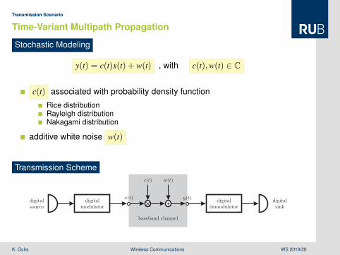
Time-Variant Multipath Propagation
Stochastic Modeling
y(t) = c(t)x(t) + w(t) , with c(t),w(t) ∈ C
c(t) associated with probability density function
Rice distributionRayleigh distributionNakagami distribution
additive white noise w(t)
Transmission Scheme
x(t)
c(t) w(t)
y(t)digitalsource
digitalmodulator
digitaldemodulator
digitalsink
baseband channel
Lehrstuhl fürDigitale Kommunikationssysteme
K. Ochs Wireless Communications WS 2019/20
Wireless Communication Channel Passband Transmission
Contents
1 Transmission Scenario
2 Passband Transmission
3 Baseband Transmission
4 Time-Discrete Transmission
Lehrstuhl fürDigitale Kommunikationssysteme
K. Ochs Wireless Communications WS 2019/20

Passband Transmission 10 / 126
Passband Transmission
Channel
real
center radian frequency ωc
bandwidth Bc
Bc
−ωc ωc ω
availablefrequency range
availablefrequency range
x0(t) y0(t)source transmitter
transmissionchannel
receiver sink
Lehrstuhl fürDigitale Kommunikationssysteme
K. Ochs Wireless Communications WS 2019/20

Passband Transmission 11 / 126
Passband Transmission
Transmission Signal
real
center radian frequency ω0
bandwidth Bx
X0(jω)
Bx
−ω0 ω0 ω
x0(t) y0(t)source transmitter
transmissionchannel
receiver sink
Lehrstuhl fürDigitale Kommunikationssysteme
K. Ochs Wireless Communications WS 2019/20
Passband Transmission 12 / 126
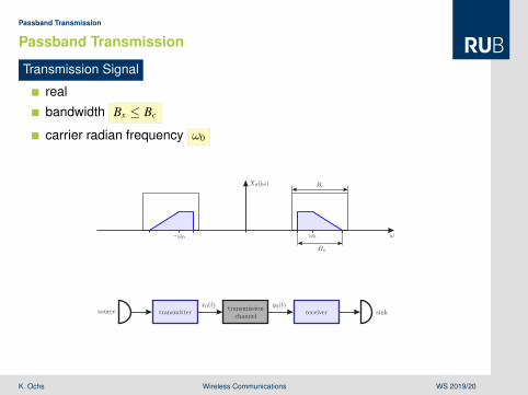
Passband Transmission
Transmission Signal
real
bandwidth Bx ≤ Bc
carrier radian frequency ω0
X0(jω) Bc
Bx
−ω0 ω0 ω
x0(t) y0(t)source transmitter
transmissionchannel
receiver sink
Lehrstuhl fürDigitale Kommunikationssysteme
K. Ochs Wireless Communications WS 2019/20

Passband Transmission 13 / 126
Passband Transmission
Equivalent Baseband
channel is complex-valued
transmitter signal x(t) is complex-valued
receiver signal y(t) is complex-valued
X(jω)
Bc
Bxω
x0(t) y0(t)x(t) y(t)digitalsource
digitalmodulator
analogmodulator
transmissionchannel
analogdemodulator
digitaldemodulator
digitalesink
baseband channel
Lehrstuhl fürDigitale Kommunikationssysteme
K. Ochs Wireless Communications WS 2019/20

Wireless Communication Channel Baseband Transmission
Contents
1 Transmission Scenario
2 Passband Transmission
3 Baseband Transmission
4 Time-Discrete Transmission
Lehrstuhl fürDigitale Kommunikationssysteme
K. Ochs Wireless Communications WS 2019/20

Baseband Transmission 14 / 126
Baseband Transmission
Channel Resources
bandwidth Bc
dynamic Dc
duration Tc
x(t) y(t)
dynamic duration
bandwidth
Dc Tc
Bc
digitalsource
digitalmodulator
basebandchannel
digitaldemodulator
digitalsink
Lehrstuhl fürDigitale Kommunikationssysteme
K. Ochs Wireless Communications WS 2019/20

Baseband Transmission 15 / 126
Baseband Transmission
Transmitter Signal
bandwidth Bx
dynamic Dx
duration Tx
x(t) y(t)
dynamic dynamicduration
duration
bandwidth bandwidth
Dx DxDcTx Tx Tc
Bx Bx
Bc
digitalsource
digitalmodulator
basebandchannel
digitaldemodulator
digitalsink
Lehrstuhl fürDigitale Kommunikationssysteme
K. Ochs Wireless Communications WS 2019/20
Baseband Transmission 16 / 126
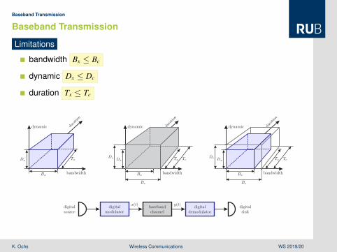
Baseband Transmission
Limitations
bandwidth Bx ≤ Bc
dynamic Dx ≤ Dc
duration Tx ≤ Tc
x(t) y(t)
dynamic dynamic dynamicduration
duration
duration
bandwidth bandwidth bandwidth
Dx Dx DxDc DcTx Tx TxTc Tc
Bx Bx Bx
Bc Bc
digitalsource
digitalmodulator
basebandchannel
digitaldemodulator
digitalsink
Lehrstuhl fürDigitale Kommunikationssysteme
K. Ochs Wireless Communications WS 2019/20

Baseband Transmission 17 / 126
Baseband Transmission
Symbol Mapping
matching of the signal dynamic Dx ≤ Dc
finite alphabet A
information in symbols u(tk) ∈ A
u(t) x(t) y(t) v(t)
dynamic dynamic dynamicduration
duration
duration
bandwidth bandwidth bandwidth
Dx Dx DxDc DcTx Tx TxTc Tc
Bx Bx Bx
Bc Bc
digitalsource
impulseshaping
basebandchannel
symbolrecovery
digitalsink
symbolmapping
inversesymbolmapping
Lehrstuhl fürDigitale Kommunikationssysteme
K. Ochs Wireless Communications WS 2019/20

Baseband Transmission 18 / 126
Baseband Transmission
Impulse Shaping
matching of the signal bandwidth Bx ≤ Bc
real pulse with finite energy q(t) ∈ R , Eq <∞crucial for symbol recovery
u(t) x(t) y(t) v(t)
dynamic dynamic dynamicduration
duration
duration
bandwidth bandwidth bandwidth
Dx Dx DxDc DcTx Tx TxTc Tc
Bx Bx Bx
Bc Bc
digitalsource
impulseshaping
basebandchannel
symbolrecovery
digitalsink
symbolmapping
inversesymbolmapping
Lehrstuhl fürDigitale Kommunikationssysteme
K. Ochs Wireless Communications WS 2019/20

Baseband Transmission 19 / 126
Transmission Scheme
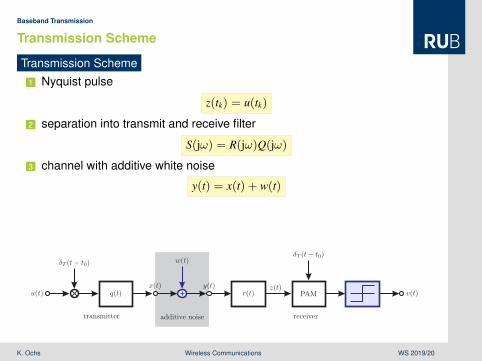
Transmission Scheme1 Nyquist pulse
z(tk) = u(tk)
2 separation into transmit and receive filter
S(jω) = R(jω)Q(jω)
3 channel with additive white noise
y(t) = x(t) + w(t)
4 optimal signal to noise ratio at decider
r(t) = q(−t)/Eq
u(t)
δT (t− t0)
s(t)z(t)
δT (t− t0)
PAM v(t)
transmitter receiver
Lehrstuhl fürDigitale Kommunikationssysteme
K. Ochs Wireless Communications WS 2019/20

Baseband Transmission 19 / 126
Transmission Scheme
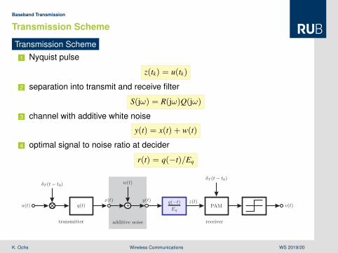
Transmission Scheme1 Nyquist pulse
z(tk) = u(tk)
2 separation into transmit and receive filter
S(jω) = R(jω)Q(jω)
3 channel with additive white noise
y(t) = x(t) + w(t)
4 optimal signal to noise ratio at decider
r(t) = q(−t)/Eq
u(t)
δT (t− t0)
q(t)x(t)
r(t)z(t)
δT (t− t0)
PAM v(t)
transmitter receiver
Lehrstuhl fürDigitale Kommunikationssysteme
K. Ochs Wireless Communications WS 2019/20
Baseband Transmission 19 / 126
Transmission Scheme
Transmission Scheme1 Nyquist pulse
z(tk) = u(tk)
2 separation into transmit and receive filter
S(jω) = R(jω)Q(jω)
3 channel with additive white noise
y(t) = x(t) + w(t)
4 optimal signal to noise ratio at decider
r(t) = q(−t)/Eq
u(t)
δT (t− t0)
q(t)x(t)
w(t)
y(t)r(t)
z(t)
δT (t− t0)
PAM v(t)
transmitter additive noise receiver
Lehrstuhl fürDigitale Kommunikationssysteme
K. Ochs Wireless Communications WS 2019/20
Baseband Transmission 19 / 126
Transmission Scheme
Transmission Scheme1 Nyquist pulse
z(tk) = u(tk)
2 separation into transmit and receive filter
S(jω) = R(jω)Q(jω)
3 channel with additive white noise
y(t) = x(t) + w(t)
4 optimal signal to noise ratio at decider
r(t) = q(−t)/Eq
u(t)
δT (t− t0)
q(t)x(t)
w(t)
y(t) q(−t)
Eq
z(t)
δT (t− t0)
PAM v(t)
transmitter additive noise receiver
Lehrstuhl fürDigitale Kommunikationssysteme
K. Ochs Wireless Communications WS 2019/20

Baseband Transmission 20 / 126
Transmission Scheme
Transmission Scheme
5 low-pass band-limited pulse
Bx ≤ Bc
6 moderate timing jitter
|τ | T
u(t)
δT (t− t0)
q(t)x(t)
w(t)
y(t) q(−t)
Eq
z(t)
δT (t− t0 − τ)
PAM v(t)
transmitter additive noise receiver
Lehrstuhl fürDigitale Kommunikationssysteme
K. Ochs Wireless Communications WS 2019/20

Baseband Transmission 21 / 126
Transmission Scheme
Transmission Scheme
7 stochastic model for flat fading and noise
8 minimizing decision error probability
transmitted u(tk) ∈ A
received z(tk − τ) ∈ C
decided v(tk) = Qz(tk − τ) ∈ A
u(t)
δT (t− t0)
q(t)x(t)
c(t) w(t)
y(t) q(−t)
Eq
z(t)
δT (t− t0 − τ)
PAM v(t)
transmitter basebandchannel
receiver
Lehrstuhl fürDigitale Kommunikationssysteme
K. Ochs Wireless Communications WS 2019/20

Baseband Transmission 21 / 126
Transmission Scheme
Transmission Scheme
7 stochastic model for flat fading and noise8 minimizing decision error probability
transmitted u(tk) ∈ A
received z(tk − τ) ∈ C
decided v(tk) = Qz(tk − τ) ∈ A
u(t)
δT (t− t0)
q(t)x(t)
c(t) w(t)
y(t) q(−t)
Eq
z(t)
δT (t− t0 − τ)
PAM v(t)
transmitter basebandchannel
receiver
Lehrstuhl fürDigitale Kommunikationssysteme
K. Ochs Wireless Communications WS 2019/20

Wireless Communication Channel Time-Discrete Transmission
Contents
1 Transmission Scenario
2 Passband Transmission
3 Baseband Transmission
4 Time-Discrete Transmission
Lehrstuhl fürDigitale Kommunikationssysteme
K. Ochs Wireless Communications WS 2019/20

Time-Discrete Transmission 22 / 126
Time-Discrete Channel
Preliminary Considerations
1 perfect timing synchronization
τ = 0
2 no receiver filter, transmitter filter is Nyquist filter
x(tk) = u(tk)
3 time-discrete channel
y(tk) = c(tk)x(tk) + w(tk)
4 decision
v(tk) = Qy(tk)
u(t)
δT (t− t0)
q(t)x(t)
c(t) w(t)
y(t) q(−t)
Eq
z(t)
δT (t− t0)
PAM v(t)
transmitter basebandchannel
receiver
Lehrstuhl fürDigitale Kommunikationssysteme
K. Ochs Wireless Communications WS 2019/20

Time-Discrete Transmission 22 / 126
Time-Discrete Channel
Preliminary Considerations
1 perfect timing synchronization
τ = 0
2 no receiver filter, transmitter filter is Nyquist filter
x(tk) = u(tk)
3 time-discrete channel
y(tk) = c(tk)x(tk) + w(tk)
4 decision
v(tk) = Qy(tk)
u(t)
δT (t− t0)
s(t)x(t)
c(t) w(t)
y(t)
δT (t− t0)
PAM v(t)
transmitter basebandchannel
receiver
Lehrstuhl fürDigitale Kommunikationssysteme
K. Ochs Wireless Communications WS 2019/20

Time-Discrete Transmission 22 / 126
Time-Discrete Channel
Preliminary Considerations
1 perfect timing synchronization
τ = 0
2 no receiver filter, transmitter filter is Nyquist filter
x(tk) = u(tk)
3 time-discrete channel
y(tk) = c(tk)x(tk) + w(tk)
4 decision
v(tk) = Qy(tk)
replacements
u(t)
δT (t− t0)
s(t)x(t)
c(t) w(t)
y(t)
δT (t− t0)
PAM v(t)
time-discrete channel
Lehrstuhl fürDigitale Kommunikationssysteme
K. Ochs Wireless Communications WS 2019/20

Time-Discrete Transmission 22 / 126
Time-Discrete Channel
Preliminary Considerations
1 perfect timing synchronization
τ = 0
2 no receiver filter, transmitter filter is Nyquist filter
x(tk) = u(tk)
3 time-discrete channel
y(tk) = c(tk)x(tk) + w(tk)
4 decision
v(tk) = Qy(tk)
u(tk) = x(tk)
c(tk) w(tk)
y(tk)v(tk)
time-discrete channel
Lehrstuhl fürDigitale Kommunikationssysteme
K. Ochs Wireless Communications WS 2019/20
Time-Discrete Transmission 23 / 126
Time-Discrete Channel
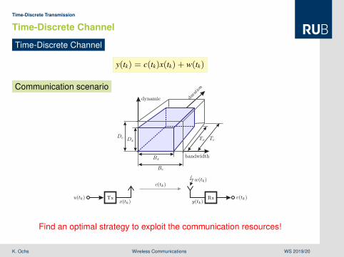
Time-Discrete Channel
y(tk) = c(tk)x(tk) + w(tk)
Communication scenariodynamic du
ration
bandwidth
DxDc Tx Tc
Bx
Bc
u(tk)x(tk)
c(tk)w(tk)
y(tk)v(tk)Tx Rx
Find an optimal strategy to exploit the communication resources!Lehrstuhl fürDigitale Kommunikationssysteme
K. Ochs Wireless Communications WS 2019/20

Time-Discrete Transmission 24 / 126
Time-Discrete Channel
Time-Discrete Channel
y(tk) = c(tk)x(tk) + w(tk)
Communication limits
U
equivo
cation
mutual information
irrelev
ance
V
u(tk)x(tk)
c(tk)w(tk)
y(tk)v(tk)Tx Rx
Use information theory to determine the communication limits!Lehrstuhl fürDigitale Kommunikationssysteme
K. Ochs Wireless Communications WS 2019/20

Wireless Communications Single Input Single Output Systems
Wireless CommunicationsSingle Input Single Output Systems
Karlheinz Ochs
Chair of Digital Communication Systems
Lehrstuhl fürDigitale Kommunikationssysteme
K. Ochs Wireless Communications WS 2019/20

Single Input Single Output Systems
Contents
1 Signal Space
2 AWGN Channel
3 Flat Fading Channel
Lehrstuhl fürDigitale Kommunikationssysteme
K. Ochs Wireless Communications WS 2019/20
Single Input Single Output Systems Signal Space
Contents
1 Signal Space
2 AWGN Channel
3 Flat Fading Channel
Lehrstuhl fürDigitale Kommunikationssysteme
K. Ochs Wireless Communications WS 2019/20
Signal Space 25 / 126
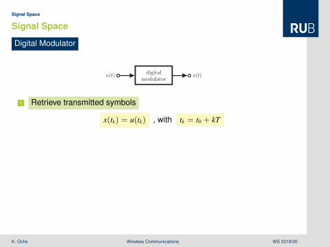
Signal Space
Digital Modulator
u(t)digital
modulatorx(t)
1 Retrieve transmitted symbols
x(tk) = u(tk) , with tk = t0 + kT
2 Nyquist criterion
s(kT) =
1 for k = 00 for k ∈ Z \ 0
3 Minimal bandwidth
s(t) = si (Ωt/2) , with ΩT = 2π
Lehrstuhl fürDigitale Kommunikationssysteme
K. Ochs Wireless Communications WS 2019/20
Signal Space 25 / 126
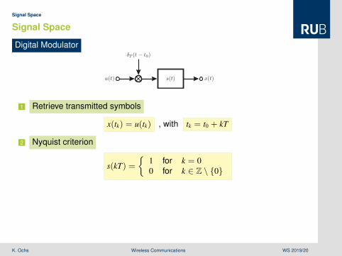
Signal Space
Digital Modulator
u(t)
δT (t− t0)
s(t) x(t)
1 Retrieve transmitted symbols
x(tk) = u(tk) , with tk = t0 + kT
2 Nyquist criterion
s(kT) =
1 for k = 00 for k ∈ Z \ 0
3 Minimal bandwidth
s(t) = si (Ωt/2) , with ΩT = 2π
Lehrstuhl fürDigitale Kommunikationssysteme
K. Ochs Wireless Communications WS 2019/20
Signal Space 25 / 126
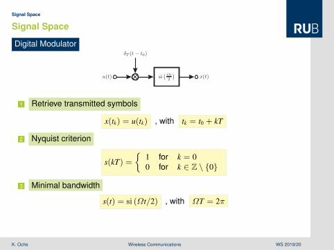
Signal Space
Digital Modulator
u(t)
δT (t− t0)
si(Ωt2
)x(t)
1 Retrieve transmitted symbols
x(tk) = u(tk) , with tk = t0 + kT
2 Nyquist criterion
s(kT) =
1 for k = 00 for k ∈ Z \ 0
3 Minimal bandwidth
s(t) = si (Ωt/2) , with ΩT = 2π
Lehrstuhl fürDigitale Kommunikationssysteme
K. Ochs Wireless Communications WS 2019/20

Signal Space 25 / 126
Signal Space
Digital Modulator
u(t)
δT (t− t0)
si(Ωt2
)x(t)
1 Retrieve transmitted symbols
x(tk) = u(tk) , with tk = t0 + kT
2 Nyquist criterion
s(kT) =
1 for k = 00 for k ∈ Z \ 0
3 Minimal bandwidth
s(t) = si (Ωt/2) , with ΩT = 2π
Signaling with Nyquist rate!Lehrstuhl fürDigitale Kommunikationssysteme
K. Ochs Wireless Communications WS 2019/20

Signal Space 26 / 126
Signal Space
Digital modulator
u(t)
δT (t− t0)
si(Ωt2
)x(t)
Digitally modulated signal
x(t) =∞∑
k=−∞
u(tk) si
(Ω
2[t − tk]
)
Lehrstuhl fürDigitale Kommunikationssysteme
K. Ochs Wireless Communications WS 2019/20

Signal Space 26 / 126
Signal Space
Digital modulator
u(t)
δT (t− t0)
si(Ωt2
)x(t)
Digitally modulated signal
x(t) =∞∑
k=−∞
xkϕk(t)
Definitions
1 samples
xk = u(tk)
2 base functions
ϕk(t) = si
(Ω
2[t − tk]
)−−• Φk(jω) = T rect
(2ωΩ
)e−jωtk
Lehrstuhl fürDigitale Kommunikationssysteme
K. Ochs Wireless Communications WS 2019/20

Signal Space 27 / 126
Signal Space
Scalar Product
〈ϕk(t), ϕ`(t)〉 =∫ ∞
−∞ϕk(t)ϕ∗` (t)dt
Orthogonal base functions
〈ϕk(t), ϕ`(t)〉 = T
1 for k = `0 for k 6= `
Proof
1 〈ϕk(t), ϕ`(t)〉 =∫ ∞−∞ ϕk(t)ϕ∗` (t)dt
2 〈ϕk(t), ϕ`(t)〉 = 12π
∫ ∞−∞ Φk(jω)Φ∗` (jω)dω
3 〈ϕk(t), ϕ`(t)〉 = 12π
∫ ∞−∞ T2 rect
( 2ωΩ
)e−jω[tk−t`]dω
4 〈ϕk(t), ϕ`(t)〉 = T 1Ω
∫ Ω/2−Ω/2 e−jω[k−`]T dω
Lehrstuhl fürDigitale Kommunikationssysteme
K. Ochs Wireless Communications WS 2019/20

Signal Space 28 / 126
Signal Space
Energy
Ex =
∫ ∞
−∞|x(t)|2dt = T
∞∑k=−∞
|xk|2
Proof
1 Ex = 〈x(t), x(t)〉 = ‖x(t)‖2
2 Ex = 〈∞∑
k=−∞xkϕk(t),
∞∑`=−∞
x`ϕ`(t)〉
3 Ex =∞∑
k=−∞
∞∑`=−∞
xkx∗` 〈ϕk(t), ϕ`(t)〉
4 Ex = T∞∑
k=−∞|xk|2
Lehrstuhl fürDigitale Kommunikationssysteme
K. Ochs Wireless Communications WS 2019/20

Signal Space 29 / 126
Signal Space
Signal Vector (finite number of symbols)
x =[
x1, x2, . . . , xK]T
power
Px =Ex
T= ‖x‖2 , with ‖x‖2 = xHx =
K∑k=1
|xk|2
law of large numbers
1K
K∑k=1
|xk|2 ≈ E|X |2
relation to stochastic power
Px ≈ KPx , with Px = E|X |2Lehrstuhl fürDigitale Kommunikationssysteme
K. Ochs Wireless Communications WS 2019/20

Single Input Single Output Systems AWGN Channel
Contents
1 Signal Space
2 AWGN Channel
3 Flat Fading Channel
Lehrstuhl fürDigitale Kommunikationssysteme
K. Ochs Wireless Communications WS 2019/20

AWGN Channel 30 / 126
Channel with Additive White Gaussian Noise
AWGN Channel
U
equivo
cation
mutual information
irrelev
ance
V
u(k)x(k)
1z(k)
y(k)v(k)Tx Rx
Remarkstransmitter sends message U to the receiver
K channel uses: Tx = KT ≤ Tc , k ∈ 1, . . . ,K
transmitter signal x(k) ∈ C with limited power Px ≤ P
additive noise z(k) ∈ C
independent and identically distributed
normal distribution, with zero mean and variance σ2z = Pz
receiver signal y(k) ∈ C
Lehrstuhl fürDigitale Kommunikationssysteme
K. Ochs Wireless Communications WS 2019/20

AWGN Channel 30 / 126
Channel with Additive White Gaussian Noise
AWGN Channel
u(k)x(k)
1z(k)
y(k)v(k)Tx Rx
Remarks
transmitter sends message U to the receiver
K channel uses: Tx = KT ≤ Tc , k ∈ 1, . . . ,K
transmitter signal x(k) ∈ C with limited power Px ≤ P
additive noise z(k) ∈ Cindependent and identically distributed
normal distribution, with zero mean and variance σ2z = Pz
receiver signal y(k) ∈ C
Lehrstuhl fürDigitale Kommunikationssysteme
K. Ochs Wireless Communications WS 2019/20

AWGN Channel 31 / 126
Channel with Additive White Gaussian Noise
AWGN Channel
Signal flow diagram
x(k)
z(k)
y(k)
Mathematical model
y(k) = x(k) + z(k) , 1 ≤ k ≤ K
Px =1K
K∑k=1
|x(k)|2 ≤ P
z(k) ∼ N (0,Pz)
Communication
encoding of message U
x(k) ∈ C is a symbol of a finite alphabet A
y(k) ∼ N (x(k),Pz)
Highest data rate for a reliable transmission?Lehrstuhl fürDigitale Kommunikationssysteme
K. Ochs Wireless Communications WS 2019/20
AWGN Channel 32 / 126
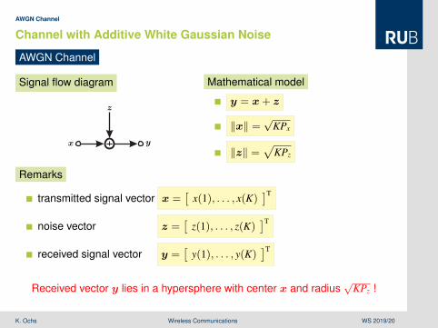
Channel with Additive White Gaussian Noise
AWGN Channel
Signal flow diagram
x
z
y
Mathematical model
y = x+ z
‖x‖ =√
KPx
‖z‖ =√
KPz
Remarks
transmitted signal vector x =[
x(1), . . . , x(K)]T
noise vector z =[
z(1), . . . , z(K)]T
received signal vector y =[
y(1), . . . , y(K)]T
Received vector y lies in a hypersphere with center x and radius√
KPz !Lehrstuhl fürDigitale Kommunikationssysteme
K. Ochs Wireless Communications WS 2019/20

AWGN Channel 33 / 126
Channel with Additive White Gaussian Noise
AWGN Channel
Illustration
xz
y0
noise hypersphere
Mathematical model
y = x+ z
E‖y‖2 = E‖x‖2+ E‖z‖2x and z are independent
Remarks
E‖y‖ ≤√E‖y‖2 , Jensen’s inequality
E‖y‖2 = E‖x‖2+ E‖z‖2 , independence
E‖x‖2 ≈ KPx , E‖z‖2 ≈ KPz , law of large numbers
Lehrstuhl fürDigitale Kommunikationssysteme
K. Ochs Wireless Communications WS 2019/20

AWGN Channel 33 / 126
Channel with Additive White Gaussian Noise
AWGN Channel
Illustration
√ KPx
√KPz
E‖y‖≤√
K[Px +Pz]
noise hypersphere
Mathematical model
y = x+ z
E‖y‖2 = E‖x‖2+ E‖z‖2x and z are independent
Upper bound
E‖y‖ ≤√
K[Px + Pz]
All received signal vectors lie in a hypersphere of radius√
K[Px + Pz]!
Lehrstuhl fürDigitale Kommunikationssysteme
K. Ochs Wireless Communications WS 2019/20

AWGN Channel 34 / 126
Channel with Additive White Gaussian Noise
AWGN Channel
Illustration
1
2
3
M
√KPz
√KPz
√KPz
√KPz
√K[Px + Pz ]
Decoding
transmitted vector x is center of thehypersphere
M nonoverlapping hypersheres
received vector y within hypershperebelongs to the center x
How many noise hyperspheres fit into the received vector hypersphere?
Lehrstuhl fürDigitale Kommunikationssysteme
K. Ochs Wireless Communications WS 2019/20

AWGN Channel 35 / 126
Channel with Additive White Gaussian Noise
AWGN Channel
Hypersphere
K (real) dimensions
radius r
volume VK(r) ∼ rK
Nonoverlapping hyperspheres
K complex dimensions
2K real dimensions
Upper bound for nonoverlapping hyperspheres
M ≤ [1 + ΓSNR]K , with ΓSNR =
Px
Pz=E|x(k)|2E|z(k)|2
Proof
M ≤ V2K(√
2K[Px + Pz])
V2K(√
2KPz)=
VK(2K[Px + Pz])
VK(2KPz)= [1 + Px/Pz]
K
Lehrstuhl fürDigitale Kommunikationssysteme
K. Ochs Wireless Communications WS 2019/20

AWGN Channel 36 / 126
Channel with Additive White Gaussian Noise
AWGN Channel
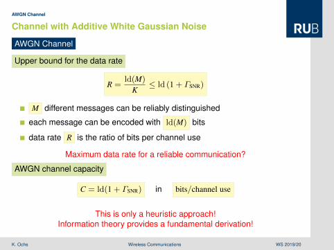
Upper bound for the data rate
R =ld(M)
K≤ ld (1 + ΓSNR)
M different messages can be reliably distinguished
each message can be encoded with ld(M) bits
data rate R is the ratio of bits per channel use
Maximum data rate for a reliable communication?
Lehrstuhl fürDigitale Kommunikationssysteme
K. Ochs Wireless Communications WS 2019/20

AWGN Channel 36 / 126
Channel with Additive White Gaussian Noise
AWGN Channel
Upper bound for the data rate
R =ld(M)
K≤ ld (1 + ΓSNR)
M different messages can be reliably distinguished
each message can be encoded with ld(M) bits
data rate R is the ratio of bits per channel use
Maximum data rate for a reliable communication?
AWGN channel capacity
C = ld(1 + ΓSNR) in bits/channel use
Lehrstuhl fürDigitale Kommunikationssysteme
K. Ochs Wireless Communications WS 2019/20
AWGN Channel 36 / 126
Channel with Additive White Gaussian Noise
AWGN Channel
Upper bound for the data rate
R =ld(M)
K≤ ld (1 + ΓSNR)
M different messages can be reliably distinguished
each message can be encoded with ld(M) bits
data rate R is the ratio of bits per channel use
Maximum data rate for a reliable communication?
AWGN channel capacity
C = ld(1 + ΓSNR) in bits/channel use
This is only a heuristic approach!Information theory provides a fundamental derivation!
Lehrstuhl fürDigitale Kommunikationssysteme
K. Ochs Wireless Communications WS 2019/20

Single Input Single Output Systems Flat Fading Channel
Contents
1 Signal Space
2 AWGN Channel
3 Flat Fading Channel
Lehrstuhl fürDigitale Kommunikationssysteme
K. Ochs Wireless Communications WS 2019/20

Flat Fading Channel 37 / 126
Flat Fading Channel
Flat Fading Channel
u(k)x(k)
h(k)z(k)
y(k)v(k)Tx Rx
Remarks
transmitter signal x(k) ∈ C with limited power Px ≤ P
channel gain h(k) ∈ Csmall-scale fading caused by echoes of the transmitted signaltransmitted signal period is larger than multi-path delay spread
additive noise z(k) ∈ Cindependent and identically distributed (i.i.d.)
normal distribution, with zero mean and variance σ2z = Pz
receiver signal y(k) ∈ C
Channel capacity?Lehrstuhl fürDigitale Kommunikationssysteme
K. Ochs Wireless Communications WS 2019/20

Flat Fading Channel 38 / 126
Flat Fading Channel
Flat Fading Channel
x(k)
h(k) z(k)z(k)
y(k)y(k) h(k)x(k)
Idea
equivalent to AWGN channel
surrogate input signal is product of input signal times channel gain
time-variant signal to noise ratio
γSNR(k) =E|h(k)x(k)|2E|z(k)|2 = ΓSNR|h(k)|2
Channel capacity
C(k) = ld(1 + ΓSNR|h(k)|2) , with ΓSNR =E|x(k)|2E|z(k)|2 =
Px
Pz
Lehrstuhl fürDigitale Kommunikationssysteme
K. Ochs Wireless Communications WS 2019/20
Flat Fading Channel 39 / 126
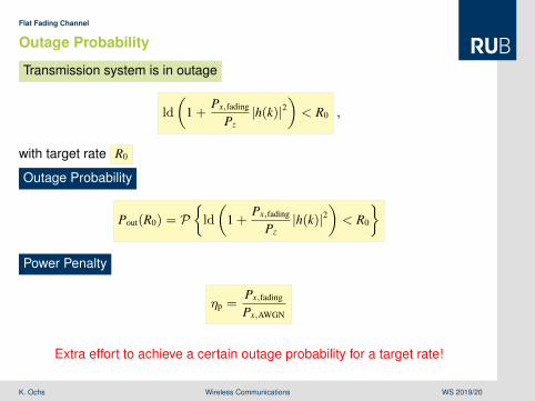
Outage Probability
Transmission system is in outage
ld
(1 +
Px,fading
Pz|h(k)|2
)< R0 ,
with target rate R0
Outage Probability
Pout(R0) = Pld
(1 +
Px,fading
Pz|h(k)|2
)< R0
Power Penalty
ηp =Px,fading
Px,AWGN
Extra effort to achieve a certain outage probability for a target rate!Lehrstuhl fürDigitale Kommunikationssysteme
K. Ochs Wireless Communications WS 2019/20

Flat Fading Channel 40 / 126
Flat Fading Channel
Rayleigh Fading
Channel gain
distribution of real and imaginary part
Reh, Imh ∼ N (0, σ2)
transformation to polar coordinates h = re jϕ
magnitude r > 0 has Rayleigh distribution
fr(r) = u(r)rσ2 e−
r2
2σ2
phase ϕ ∈ (−π, π] has uniform distribution
fϕ(ϕ) =1
2πrect
(ϕπ
)Real- and imaginary part have zero-mean, which indicates no line of sight!
Lehrstuhl fürDigitale Kommunikationssysteme
K. Ochs Wireless Communications WS 2019/20

Flat Fading Channel 41 / 126
Flat fading Channel
Rayleigh Distribution (σ = 1)
0 0.5 1 1.5 2 2.5 3 3.5 4 4.5 50
0.1
0.2
0.3
0.4
0.5
0.6
0.7
r
f r(r)
Lehrstuhl fürDigitale Kommunikationssysteme
K. Ochs Wireless Communications WS 2019/20

Flat Fading Channel 42 / 126
Flat Fading Channel
Rician Fading
Channel gain
distribution of real and imaginary part
Reh ∼ N (µRe, σ2) , Imh ∼ N (µIm, σ
2)
transformation to polar coordinates h = re jϕ
magnitude r > 0 has Rice distribution
fr(r) = u(r)rσ2 I0
( rµσ2
)e−
r2+µ2
2σ2 , with µ =√µ2
Re + µ2Im
and modified Bessel function of the first kind with order zero I0
Rician factor K =µ
2σ2
K = 0 yields Rayleigh fading
Line of sight if Rician factor is greater than zero!Lehrstuhl fürDigitale Kommunikationssysteme
K. Ochs Wireless Communications WS 2019/20

Flat Fading Channel 43 / 126
Flat Fading Channel
Rician Distribution (σ = 1)
0 1 2 3 4 5 6 7 80
0.1
0.2
0.3
0.4
0.5
0.6
0.7
r
f r(r)
µ = 0µ = 0.5µ = 1µ = 2µ = 4
Lehrstuhl fürDigitale Kommunikationssysteme
K. Ochs Wireless Communications WS 2019/20

Flat Fading Channel 44 / 126
Flat Fading Channel
Nakagami Fading
Channel gainsum of multiple i.i.d. Rayleigh fading signals has Nakagami distributedmagnitudemagnitude r > 0 has Nakagami distribution
fr(r) = u(r)2
Γ (m)
[mΩ
]mr2m−1 e−
mr2Ω ,
with
gamma function Γ (m) =
∫ ∞0
e−rrm−1dr
received signal average power Ω = Er2
shape factor m =Ω2
E[r −Ω]2≥
12
m = 1 yields Rayleigh fading
Useful to model urban radio multipath channels!Lehrstuhl fürDigitale Kommunikationssysteme
K. Ochs Wireless Communications WS 2019/20

Flat Fading Channel 45 / 126
Flat Fading Channel
Nakagami Distribution
0 0.2 0.4 0.6 0.8 1 1.2 1.4 1.6 1.8 2 2.2 2.4 2.6 2.8 30
0.2
0.4
0.6
0.8
1
1.2
1.4
r
f r(r
)
Ω = 1,m = 0.5Ω = 1,m = 1Ω = 2,m = 1Ω = 3,m = 1Ω = 1,m = 2Ω = 2,m = 2Ω = 1,m = 3
Lehrstuhl fürDigitale Kommunikationssysteme
K. Ochs Wireless Communications WS 2019/20

Wireless Communications Multiple Input Multiple Output Systems
Wireless CommunicationsMultiple Input Multiple Output Systems
Karlheinz Ochs
Chair of Digital Communication Systems
Lehrstuhl fürDigitale Kommunikationssysteme
K. Ochs Wireless Communications WS 2019/20

Multiple Input Multiple Output Systems
Contents
1 Transmission Scenario
2 MIMO Detectors
3 Random Channels
4 Eigenmode Decomposition
5 Capacity and Degrees of Freedom
Lehrstuhl fürDigitale Kommunikationssysteme
K. Ochs Wireless Communications WS 2019/20
Multiple Input Multiple Output Systems Transmission Scenario
Contents
1 Transmission Scenario
2 MIMO Detectors
3 Random Channels
4 Eigenmode Decomposition
5 Capacity and Degrees of Freedom
Lehrstuhl fürDigitale Kommunikationssysteme
K. Ochs Wireless Communications WS 2019/20

Transmission Scenario 46 / 126
MIMO Passband Transmitter
MIMO Passband Transmitter
u(t)
S
P
symbolmapping
symbolmapping
δT (t− t0)
δT (t− t0)
q(t)
q(t)
ejω0t
ejω0t
Re
Re
u1(t)
um(t)
x1(t)
xm(t)
x10(t)
xm0(t)
Lehrstuhl fürDigitale Kommunikationssysteme
K. Ochs Wireless Communications WS 2019/20

Transmission Scenario 47 / 126
MIMO Passband Receiver
MIMO Passband Receiver
PAM
PAM
e−jω0t
e−jω0t
LP
LP
r(t)
r(t)
δT (t− t0)
δT (t− t0)
detection
v(t)
w10(t)
wn0(t)
y10(t)
yn0(t)
y1(t)
yn(t)
v1(t)
vn(t)
Instead of single decisions a combined detection of transmitted symbols!Lehrstuhl fürDigitale Kommunikationssysteme
K. Ochs Wireless Communications WS 2019/20

Transmission Scenario 48 / 126
MIMO passband transmission
MIMO Passband Transmitterm transmit antennas
symbol vector u(tk) ∈ Am , with u(t) =[
u1(t), . . . , um(t)]T
equivalent low-pass signal vector x(t) =∞∑
k=−∞
u(tk)q(t − tk)
baseband signal vector x0(t) = Rex(t)e jω0t
,
with x0(t) =[
x10(t), . . . , xm0(t)]T
MIMO Passband Receivern receive antennas
additive noise w0(t) =[
w10(t), . . . ,wn0(t)]T
baseband signal y0(t) =[
y10(t), . . . , yn0(t)]T
Lehrstuhl fürDigitale Kommunikationssysteme
K. Ochs Wireless Communications WS 2019/20

Transmission Scenario 49 / 126
MIMO Baseband Transmission
MIMO Baseband Transmission
AM
AM
u(t)
S
P
P
P
symbolmapping
symbolmapping
δT (t− t0)
δT (t− t0)
δT (t− t0)
δT (t− t0)
q(t)
q(t)
u1(t)
um(t)
x1(t)
xm(t)
c11(t)
cn1(t)
c1m(t)
cnm(t)
r(t)
r(t)
detection
v(t)
w1(t)
wn(t)
y1(t)
yn(t)
v1(t)
vn(t)
Lehrstuhl fürDigitale Kommunikationssysteme
K. Ochs Wireless Communications WS 2019/20

Transmission Scenario 50 / 126
MIMO Baseband Transmission (simplified)
MIMO Baseband Transmission (simplified)
AM
AM
u(t)
S
P
P
P
symbolmapping
symbolmapping
δT (t− t0)
δT (t− t0)
δT (t− t0)
δT (t− t0)
s(t)
s(t)
u1(t)
um(t)
x1(t)
xm(t)
h11(t)
hn1(t)
h1m(t)
hnm(t)
detection
v(t)
z1(t)
zn(t)
y1(t)
yn(t)
v1(t)
vn(t)
Lehrstuhl fürDigitale Kommunikationssysteme
K. Ochs Wireless Communications WS 2019/20

Transmission Scenario 51 / 126
MIMO Digital Baseband Transmission
MIMO Digital Baseband Transmission
u(k)
x1(k)
xm(k)
h11(k)
hn1(k)
h1m(k)
hnm(k)
z1(k)
zn(k)
y1(k)
yn(k)
v(k)Tx Rx
Flat fading channel
y1(k)...
yn(k)
=
h11(k) · · · h1m(k)...
. . ....
hn1(k) · · · hnm(k)
x1(k)
...xm(k)
+
z1(k)...
zn(k)
Lehrstuhl fürDigitale Kommunikationssysteme
K. Ochs Wireless Communications WS 2019/20

Transmission Scenario 52 / 126
MIMO Digital Baseband Transmission
MIMO Digital Baseband Transmission
u(k) Txx(k)
H(k)z(k)
y(k)Rx v(k)
Transmitter
maps message U to signal x(k)
transmitter signal has limited power
Flat fading channel
y(k) =H(k)x(k) + z(k)
channel matrix has almost sure full rankReceiver
knows the channel state from estimationretrieves message V from signal y(k)
Channel capacity?Lehrstuhl fürDigitale Kommunikationssysteme
K. Ochs Wireless Communications WS 2019/20

Multiple Input Multiple Output Systems MIMO Detectors
Contents
1 Transmission Scenario
2 MIMO DetectorsZero-Forcing DetectorMinimum Mean-Squared Error DetectorMaximum Likelihood Detector
3 Random Channels
4 Eigenmode Decomposition
5 Capacity and Degrees of Freedom
Lehrstuhl fürDigitale Kommunikationssysteme
K. Ochs Wireless Communications WS 2019/20

MIMO Detectors 53 / 126
MIMO Detectors
MIMO Detector
x(k)
H(k) z(k)
y(k) MIMO-detector
x(k)
Remarks
m transmit and n receive antennas
flat fading channel
y(k) =H(k)x(k) + z(k)
channel matrix has (almost sure) full rank
H(k) ∈ Cn×m , with rankH(k) = minm, n
MIMO detector estimates transmitted signalLehrstuhl fürDigitale Kommunikationssysteme
K. Ochs Wireless Communications WS 2019/20

MIMO Detectors Zero-Forcing Detector 54 / 126
Zero-Forcing Detector
Scenario 1same number of antennas at transmitter and receiverrank(H(k)) = m = n
equation system
x(k)H(k) z(k)y(k) +=
Zero-Forcing Detection
x =H−1y ⇒ x = x+H−1z
Remarkssimple case
multiplication with H−1 can significantly amplify the noiseLehrstuhl fürDigitale Kommunikationssysteme
K. Ochs Wireless Communications WS 2019/20
MIMO Detectors Zero-Forcing Detector 55 / 126
Zero-Forcing Detector
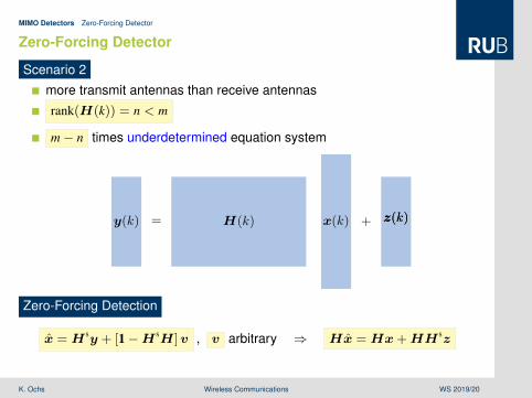
Scenario 2
more transmit antennas than receive antennas
rank(H(k)) = n < m
m− n times underdetermined equation system
x(k)H(k) z(k)z(k)y(k) +=
Zero-Forcing Detection
x =H sy + [1−H sH]v , v arbitrary ⇒ Hx =Hx+HH sz
Lehrstuhl fürDigitale Kommunikationssysteme
K. Ochs Wireless Communications WS 2019/20

MIMO Detectors Zero-Forcing Detector 56 / 126
Zero-Forcing Detector
Remarks
semi-inverse H s , with HH sH =H and H sHH s =H s
Moore-Penrose right pseudoinverse can be used
H s =H+ =HH[HHH]−1
1−H sH is projection matrix to null space of H
Hx =HH sy
multiplication with HH s can significantly amplify the noise
Improper approach because of infinite many solutions!
Remedy
time variance of the channel is helpful
sent x again to increase number of linearly independent equationsLehrstuhl fürDigitale Kommunikationssysteme
K. Ochs Wireless Communications WS 2019/20

MIMO Detectors Zero-Forcing Detector 57 / 126
Zero-Forcing Detector
Scenario 3
more receive antennas than transmit antennas
rank(H(k)) = m < n
n− m times overdetermined equation system
x(k)H(k) z(k)z(k)y(k) +=
Zero-Forcing Detection
x =H+y ⇒ x = x+H+z
Lehrstuhl fürDigitale Kommunikationssysteme
K. Ochs Wireless Communications WS 2019/20

MIMO Detectors Zero-Forcing Detector 58 / 126
Zero-Forcing Detector
Remarks
Moore-Penrose left pseudoinverse H+ = [HHH]−1HH
multiplication with H+ can significantly amplify the noise
Solution is an optimal approximation!
Optimization problem
x = argminxJ
, with J = ‖y −Hx‖2
Lehrstuhl fürDigitale Kommunikationssysteme
K. Ochs Wireless Communications WS 2019/20

MIMO Detectors Zero-Forcing Detector 59 / 126
Zero-Forcing Detector
Solution
necessary and sufficient conditions
∂J∂x
= 0T and∂J∂xH = 0
Wirtinger derivatives, x and xH independent
J = J∗ ⇒ ∂J∂x
=
[∂J∂xH
]H
,∂J∂x
= 0T ⇔ ∂J∂xH = 0
J = [yH − xHHH][y −Hx]
∂J∂xH = −HH[y −Hx]
HHy =HHHx
x =[HHH
]−1HHy
Lehrstuhl fürDigitale Kommunikationssysteme
K. Ochs Wireless Communications WS 2019/20

MIMO Detectors Minimum Mean-Squared Error Detector 60 / 126
Minimum Mean-Squared Error Detector
Detection
x =Dy , with y =Hx+ z
A minimum mean-squared error detector considers noise!
Optimization problem
D = argminDJ
, with J = E‖x− x‖2
Approach
J = J∗
necessary and sufficient conditions
∂J∂D
= 0T and∂J∂DH = 0
Wirtinger derivatives, D and DH independentLehrstuhl fürDigitale Kommunikationssysteme
K. Ochs Wireless Communications WS 2019/20

MIMO Detectors Minimum Mean-Squared Error Detector 61 / 126
Minimum Mean-Squared Error Detector
Realness
J = J∗
necessary and sufficient condition
∂J∂DH = 0
Some basics
‖x‖2 = xHx = tr(xxH)
Kxy = ExyH
E‖x‖2
= tr (Kxx)
∂
∂Mtr (AMB) = ATBT
Lehrstuhl fürDigitale Kommunikationssysteme
K. Ochs Wireless Communications WS 2019/20
MIMO Detectors Minimum Mean-Squared Error Detector 62 / 126
Minimum Mean-Squared Error Detector
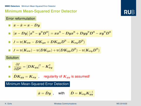
Error reformulation
x− x = x−Dy
[x−Dy][xH − yHDH] = xxH −DyxH +DyyHDH − xyHDH
J = tr(Kxx −DKyx +DKyyDH −KxyD
H)
J = tr(Kxx)− tr(DKyx) + tr(DKyyDH)− tr(KxyD
H)
Solution
∂J∂DH = [DKyy]
T −KTxy
DKyy =Kxy , regularity of Kyy is assumed!
Minimum Mean-Squared Error Detection
x = Dy , with D =KxyK−1yy
Lehrstuhl fürDigitale Kommunikationssysteme
K. Ochs Wireless Communications WS 2019/20
MIMO Detectors Minimum Mean-Squared Error Detector 63 / 126
Minimum Mean-Squared Error Detector
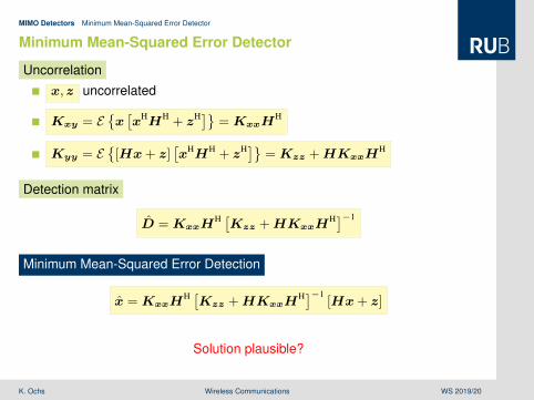
Uncorrelation
x,z uncorrelated
Kxy = Ex[xHHH + zH] =KxxH
H
Kyy = E[Hx+ z]
[xHHH + zH] =Kzz +HKxxH
H
Detection matrix
D =KxxHH [Kzz +HKxxH
H]−1
Minimum Mean-Squared Error Detection
x =KxxHH [Kzz +HKxxH
H]−1[Hx+ z]
Solution plausible?
Lehrstuhl fürDigitale Kommunikationssysteme
K. Ochs Wireless Communications WS 2019/20
MIMO Detectors Minimum Mean-Squared Error Detector 64 / 126
Minimum Mean-Squared Error Detector
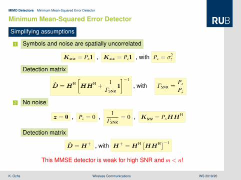
Simplifying assumptions
1 Symbols and noise are spatially uncorrelated
Kxx = Px1 , Kzz = Pz1 , with Pz = σ2z
Detection matrix
D =HH[HHH +
1ΓSNR
1]−1
, with ΓSNR =Px
Pz
2 No noise
z = 0 , Pz = 0 ,1
ΓSNR= 0 , Kyy = PxHH
H
Detection matrix
D =H+ , with H+ =HH [HHH]−1
This MMSE detector is weak for high SNR and m < n!Lehrstuhl fürDigitale Kommunikationssysteme
K. Ochs Wireless Communications WS 2019/20

MIMO Detectors Maximum Likelihood Detector 65 / 126
Maximum Likelihood Detector
Stochastic Channel Model
y =Hx+ z , with known fy|x(y|x)
Detection
x = argmaxx∈Am fy|x(y|x)
Interpretation
fy|x(y|x) ≥ fy|x(y|x) for all x ∈ Am
A maximum likelihood detector chooses the most likely sent x!
Lehrstuhl fürDigitale Kommunikationssysteme
K. Ochs Wireless Communications WS 2019/20

MIMO Detectors Maximum Likelihood Detector 66 / 126
Maximum Likelihood Detector
Reformulation
z = y −Hx
fy|x(y|x) = fz(y −Hx)
Maximum Likelihood Detection
x = argmaxx∈Am fz(y −Hx)
Simplifying assumptions
1 circularly symmetric complex Gaussian random variables
fz =1
det(πKzz)exp
(−zHK−1
zzz)
2 spatially uncorrelated noise
Kzz = Pz1 , with Pz = σ2z
Lehrstuhl fürDigitale Kommunikationssysteme
K. Ochs Wireless Communications WS 2019/20

MIMO Detectors Maximum Likelihood Detector 67 / 126
Maximum Likelihood Detector
Intermediate results
fz =1
[πσ2z ]n
exp
(− 1σ2
z‖z‖2
)
x = argmaxx∈Am
1
[πσ2z ]n
exp
(− 1σ2
z‖y −Hx‖2
)Exponential function is strictly monotonically increasing!
Maximum Likelihood Detection
x = argminx∈Am
‖y −Hx‖
Remarksgeometrical task to find x ∈ Am, such that Hx has minimal distance to ythere are |A|m possible vectors x ∈ Am
Effort increases exponentially with the number of transmit antennas!Lehrstuhl fürDigitale Kommunikationssysteme
K. Ochs Wireless Communications WS 2019/20

Multiple Input Multiple Output Systems Random Channels
Contents
1 Transmission Scenario
2 MIMO Detectors
3 Random ChannelsSpatially Uncorrelated ChannelSpatially Correlated Channel
4 Eigenmode Decomposition
5 Capacity and Degrees of Freedom
Lehrstuhl fürDigitale Kommunikationssysteme
K. Ochs Wireless Communications WS 2019/20

Random Channels 68 / 126
Random MIMO Channel
Random MIMO Channel
x(k)
H(k) z(k)
y(k)
flat fading (frequency-non-selective)
channel matrix H(k) has (almost sure) full rank
elements hµν(k) of H(k) are random variables
Random channel matrix!
Example
no line of sight between transmit antenna µ and receive antenna ν
modeled e. g. with Rayleigh-distributed |hνµ(k)|Lehrstuhl fürDigitale Kommunikationssysteme
K. Ochs Wireless Communications WS 2019/20
Random Channels Spatially Uncorrelated Channel 69 / 126
Spatially Uncorrelated Channel
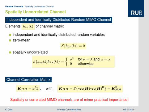
Independent and Identically Distributed Random MIMO Channel
Elements hµν(k) of channel matrix
independent and identically distributed random variableszero-mean
Ehµν(k) = 0
spatially uncorrelated
Ehνµ(k)hλκ(k) =σ2 for ν = λ and µ = κ0 otherwise
Channel Correlation Matrix
KHH = σ21 , with KHH = E
vec(H)vec(H)H =KHHH
Spatially uncorrelated MIMO channels are of minor practical importance!Lehrstuhl fürDigitale Kommunikationssysteme
K. Ochs Wireless Communications WS 2019/20

Random Channels Spatially Correlated Channel 70 / 126
Spatially Correlated Channel
Dense antenna array
improved directional characteristiccorrelation between antenna signals
Spatially Correlated Channel
x(k)
√Kx(k) HIID(k)
√Ky(k)
Hz(k)
y(k)
at transmitter Kx =KHx ≥ 0 , with Kx =
√Kx
H√Kx
at receiver Ky =KHy ≥ 0 , with Ky =
√Ky
H√Ky
Random channel matrix
H =√Ky
HHIID√Kx
Lehrstuhl fürDigitale Kommunikationssysteme
K. Ochs Wireless Communications WS 2019/20
Random Channels Spatially Correlated Channel 71 / 126
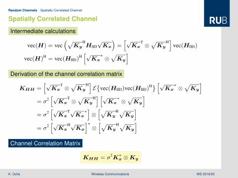
Spatially Correlated Channel
Intermediate calculations
vec(H) = vec(√
KyHHIID√Kx
)=[√Kx
T ⊗√Ky
H]
vec(HIID)
vec(H)H = vec(HIID)H[√Kx∗ ⊗
√Ky
]Derivation of the channel correlation matrix
KHH =[√Kx
T ⊗√Ky
H]E
vec(HIID)vec(HIID)H [√Kx
∗ ⊗√Ky
]= σ2
[√Kx
T ⊗√Ky
H] [√
Kx∗ ⊗
√Ky
]= σ2
[√Kx
T√Kx∗]⊗[√Ky
H√Ky
]= σ2
[√Kx
H√Kx
]∗⊗[√Ky
H√Ky
]Channel Correlation Matrix
KHH = σ2K∗x ⊗Ky
Lehrstuhl fürDigitale Kommunikationssysteme
K. Ochs Wireless Communications WS 2019/20

Multiple Input Multiple Output Systems Eigenmode Decomposition
Contents
1 Transmission Scenario
2 MIMO Detectors
3 Random Channels
4 Eigenmode DecompositionSingular Value DecompositionEigenmodes of a MIMO Channel
5 Capacity and Degrees of Freedom
Lehrstuhl fürDigitale Kommunikationssysteme
K. Ochs Wireless Communications WS 2019/20

Eigenmode Decomposition Singular Value Decomposition 72 / 126
Singular Value Decomposition
Singular Value Decomposition
H = UΣV H =[U1 U2
] [ Σr 00 0
] [V H
1
V H2
],
with
H ∈ Cn×m , r = rank(H) ≤ minm, n
U ∈ Cn×n , UHU = UUH = 1n , U1 ∈ Cn×r , U2 ∈ Cn×n−r
V ∈ Cm×m , V HV = V V H = 1m , V1 ∈ Cm×r , V2 ∈ Cm×m−r
Σ ∈ Cn×m , Σr = diag(σ1, . . . , σr) > 0
For every matrix H ∈ Cn×m with rank r there exists asingular value decomposition with positive singular values σ1, . . . , σr!
Lehrstuhl fürDigitale Kommunikationssysteme
K. Ochs Wireless Communications WS 2019/20

Eigenmode Decomposition Eigenmodes of a MIMO Channel 73 / 126
Eigenmodes of a MIMO Channel
Scenario
PSfrag
x(k)Pre-
Encoder
x′(k)
H(k) z′(k)
y′(k)Post-
Encodery(k)
Transmitter has channel state information (CSIT)!
Channel
y′ =Hx′ + z′
Encoders
use encoders to decouple transmission paths
exploit singular value decomposition
H = UΣV H ⇔ UHHV = Σ
Lehrstuhl fürDigitale Kommunikationssysteme
K. Ochs Wireless Communications WS 2019/20
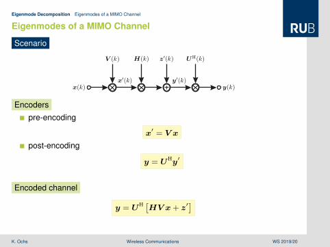
Eigenmode Decomposition Eigenmodes of a MIMO Channel 74 / 126
Eigenmodes of a MIMO Channel
Scenario
PSfrag
x(k)
V (k)
x′(k)
H(k) z′(k)
y′(k)
UH(k)
y(k)
Encoders
pre-encoding
x′ = V x
post-encoding
y = UHy′
Encoded channel
y = UH [HV x+ z′]
Lehrstuhl fürDigitale Kommunikationssysteme
K. Ochs Wireless Communications WS 2019/20

Eigenmode Decomposition Eigenmodes of a MIMO Channel 75 / 126
Eigenmodes of a MIMO Channel
Scenario
x(k)
V (k)
x′(k)
H(k) UH(k) UH(k)z′(k)
y(k)
Equivalent channel
y = UHHV x+UHz′
Lehrstuhl fürDigitale Kommunikationssysteme
K. Ochs Wireless Communications WS 2019/20

Eigenmode Decomposition Eigenmodes of a MIMO Channel 75 / 126
Eigenmodes of a MIMO Channel
Scenario
x(k)
Σ(k) z(k)
y(k)
Equivalent channel
y = Σx+ z ,
with
encoded channel
Σ = UHHV
encoded noise
z = UHz′ , with ‖z‖2 =∥∥z′∥∥2
Noise power conserved after unitary transformation!Lehrstuhl fürDigitale Kommunikationssysteme
K. Ochs Wireless Communications WS 2019/20

Eigenmode Decomposition Eigenmodes of a MIMO Channel 75 / 126
Eigenmodes of a MIMO Channel
Scenario
x(k)
Σ(k) z(k)
y(k)
Equivalent channel
y = Σx+ z
[yr
yn−r
]=
[Σr 00 0
] [xr
xm−r
]+
[zr
zn−r
]
yν = σνxν + zν for ν = 1, . . . , ryν = zν for ν = r + 1, . . . , n
Encoding yields r (relevant) parallel SISO channels!
Lehrstuhl fürDigitale Kommunikationssysteme
K. Ochs Wireless Communications WS 2019/20

Eigenmode Decomposition Eigenmodes of a MIMO Channel 76 / 126
Eigenmodes of a MIMO Channel
Unitary transformation
Noise with circularly-symmetric and zero mean complex normal distribution
z = UHz′
z′ ∼ N (0,Kz′z′) i. e. f ′z(z) =exp
(−zHK−1
z′z′z)
|πKz′z′ |
z ∼ N (0,Kzz) , Kzz = UHKz′z′U
In addition, spatially uncorrelated with identical power
Kz′z′ = σ2z 1
z ∼ N(
0, σ2z 1)
, Kzz =Kz′z′
Stochastic properties conserved after unitary transformation!Lehrstuhl fürDigitale Kommunikationssysteme
K. Ochs Wireless Communications WS 2019/20

Multiple Input Multiple Output Systems Capacity and Degrees of Freedom
Contents
1 Transmission Scenario
2 MIMO Detectors
3 Random Channels
4 Eigenmode Decomposition
5 Capacity and Degrees of FreedomCapacityDegrees of Freedom
Lehrstuhl fürDigitale Kommunikationssysteme
K. Ochs Wireless Communications WS 2019/20

Capacity and Degrees of Freedom Capacity 77 / 126
Capacity of SISO Channels
Capacity of SISO Channels
AWGN channel
x(k)
z(k)
y(k)
C = ld(1 + ΓSNR) , with ΓSNR =Px
Pz=E|x(k)|2E|z(k)|2
Flat fading channel
x(k)
h(k) z(k)
y(k)
C(k) = ld(1 + ΓSNR|h(k)|2)
Capacity of a MIMO channel?Lehrstuhl fürDigitale Kommunikationssysteme
K. Ochs Wireless Communications WS 2019/20

Capacity and Degrees of Freedom Capacity 78 / 126
Capacity of MIMO Channels
Capacity of a Decomposed MIMO Channel
Parallel SISO channels
x (k)
σ (k) z(k)
y(k)
y%(k) = σ%(k) x%(k) + z%(k) for % = 1, . . . , r
Simplifying assumption
ΓSNR =E|x%(k)|2E|z%(k)|2
Capacity
C(k) =r∑
%=1
C%(k) , with C%(k) = ld(
1 + ΓSNRσ2% (k)
)Reformulation independent from singular value decomposition?
Lehrstuhl fürDigitale Kommunikationssysteme
K. Ochs Wireless Communications WS 2019/20

Capacity and Degrees of Freedom Capacity 79 / 126
Capacity of MIMO Channels
Capacity of a Decomposed MIMO Channel
C(k) =r∑
%=1
ld(
1 + ΓSNRσ2% (k)
)
Refomulation
1r∑
%=1ld(ξ%) = ld
(r∏
%=1ξ%
)
C(k) = ld
(r∏
%=1
[1 + ΓSNRσ
2% (k)
])
2r∏
%=1ξ% = |diag(ξ%)|
C(k) = ld(∣∣∣diag
(1 + ΓSNRσ
2% (k)
)∣∣∣)Lehrstuhl fürDigitale Kommunikationssysteme
K. Ochs Wireless Communications WS 2019/20

Capacity and Degrees of Freedom Capacity 80 / 126
Capacity of MIMO Channels
Refomulation
3 diag(1 + ξ%) = 1 + diag(ξ%) , diag(αξ%) = α diag(ξ%) ,
C(k) = ld(∣∣∣1 + ΓSNR diag
(σ2% (k)
)∣∣∣)4 diag(ξ2
%) = diag(ξ%)2
C(k) = ld(∣∣∣1 + ΓSNRΣ
2r (k)
∣∣∣)
5
∣∣∣∣[ A 00 1
]∣∣∣∣ = |A|C(k) = ld
(∣∣1m + ΓSNRΣH(k)Σ(k)
∣∣)6 HHH = V ΣHΣV H i. e. ΣHΣ = V HHHHV
C(k) = ld(∣∣V H(k)
[1m + ΓSNRH
H(k)H(k)]V (k)
∣∣)Lehrstuhl fürDigitale Kommunikationssysteme
K. Ochs Wireless Communications WS 2019/20

Capacity and Degrees of Freedom Capacity 81 / 126
Capacity of MIMO Channels
Refomulation
7 |AB| = |A| |B| ,∣∣A−1
∣∣ = |A|−1
C(k) = ld(∣∣1m + ΓSNRH
H(k)H(k)∣∣)
8 |1n +AB| = |1m +BA| for A ∈ Cn×m , B ∈ Cm×n
C(k) = ld(∣∣1n + ΓSNRH(k)HH(k)
∣∣)Hint
m ≤ n
C(k) = ld(∣∣1m + ΓSNRH
H(k)H(k)∣∣)
n ≤ m
C(k) = ld(∣∣1n + ΓSNRH(k)HH(k)
∣∣)No need for singular value decomposition!
Lehrstuhl fürDigitale Kommunikationssysteme
K. Ochs Wireless Communications WS 2019/20

Capacity and Degrees of Freedom Capacity 82 / 126
Capacity of MIMO Channels
Capacity of a MIMO Channel
C(k) = maxKxx
ld(∣∣Kzz +HKxxH
H∣∣)− ld (|Kzz|)
s. t. trace(Kxx) ≤ P
This is a (convex) optimization problem!
Special case
Kxx = Px1 , Kzz = σ2z 1 , ΓSNR =
Px
σ2z
C(k) = ld(∣∣1n + ΓSNRH(k)HH(k)
∣∣)Capacity of r parallel SISO channels with constant signal to noise ratio!
Lehrstuhl fürDigitale Kommunikationssysteme
K. Ochs Wireless Communications WS 2019/20

Capacity and Degrees of Freedom Degrees of Freedom 83 / 126
Degrees of Freedom
Degrees of Freedom
η = limΓSNR→∞
Cld(ΓSNR)
average of symbols per channel use
synonymous DoF
closely related to multiplexing gain
SISO channel
η = 1
MIMO channel
η = r
The degrees of freedoms are equal to the rank of the channel matrix!Lehrstuhl fürDigitale Kommunikationssysteme
K. Ochs Wireless Communications WS 2019/20
Capacity and Degrees of Freedom Degrees of Freedom 84 / 126
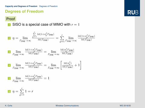
Degrees of Freedom
Proof
1 SISO is a special case of MIMO with r = 1
2 η = limΓSNR→∞
r∑%=1
ld(1+σ2%ΓSNR)
ld(ΓSNR)=
r∑%=1
limΓSNR→∞
ld(1+σ2%ΓSNR)
ld(ΓSNR)
3 limΓSNR→∞
ld(1+σ2%ΓSNR)
ld(ΓSNR)= limΓSNR→∞
ld(σ2%ΓSNR)
ld(ΓSNR)
4 limΓSNR→∞
ld(1+σ2%ΓSNR)
ld(ΓSNR)= limΓSNR→∞
[ld(σ2
%)
ld(ΓSNR)+ 1]
5 limΓSNR→∞
ld(1+σ2%ΓSNR)
ld(ΓSNR)= 1
6 η =r∑
%=11 = r
Lehrstuhl fürDigitale Kommunikationssysteme
K. Ochs Wireless Communications WS 2019/20

Capacity and Degrees of Freedom Degrees of Freedom 85 / 126
Degrees of Freedom
Degrees of Freedom
η = limΓSNR→∞
Cld(ΓSNR)
Interpretation
η = limΓSNR→∞
CCSISO
, with CSISO = ld(1 + |σ|2ΓSNR)
Multiplexing Gain
C ≈ ηCSISO for ΓSNR →∞
Asymptotic measurement for the high signal to noise ratio regime!
Lehrstuhl fürDigitale Kommunikationssysteme
K. Ochs Wireless Communications WS 2019/20

Wireless Communications Optimal Transmission Strategies
Wireless CommunicationsOptimal Transmission Strategies
Karlheinz Ochs
Chair of Digital Communication Systems
Lehrstuhl fürDigitale Kommunikationssysteme
K. Ochs Wireless Communications WS 2019/20

Optimal Transmission Strategies
Contents
1 Maximum Ratio Combining
2 Maximum Ratio Transmission
3 Water-Filling
Lehrstuhl fürDigitale Kommunikationssysteme
K. Ochs Wireless Communications WS 2019/20
Optimal Transmission Strategies Maximum Ratio Combining
Contents
1 Maximum Ratio Combining
2 Maximum Ratio Transmission
3 Water-Filling
Lehrstuhl fürDigitale Kommunikationssysteme
K. Ochs Wireless Communications WS 2019/20
Maximum Ratio Combining 86 / 126
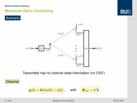
Maximum Ratio Combining
Scenario
w(k) Txx(k)
h1(k)
hn(k)
z1(k)
zn(k)
y1(k)
yn(k)
Rx w(k)
Transmitter has no channel state information (no CSIT)
Channel
y(k) = h(k)x(k) + z(k) , with Kzz = σ2z 1
Lehrstuhl fürDigitale Kommunikationssysteme
K. Ochs Wireless Communications WS 2019/20

Maximum Ratio Combining 87 / 126
Maximum Ratio Combining
Strategy
x(k) = hH(k)y(k)
Channel with strategy
x(k)
‖h(k)‖2 hH(k)z(k)
x(k)
x(k) = ‖h(k)‖2x(k) + hH(k)z(k)
Maximum achievable data rate?
Lehrstuhl fürDigitale Kommunikationssysteme
K. Ochs Wireless Communications WS 2019/20

Maximum Ratio Combining 88 / 126
Maximum Ratio Combining
Signal to noise ratio
γSNR = E|‖h‖2x|2E|hHz|2 = ‖h‖4E|x|2
EhHzzHh = ‖h‖4PxhHKzzh
= ‖h‖4Pxσ2
zhHh
= ‖h‖2ΓSNR
Achievable data rate
R(k) ≤ Rmax(k) = ld(
1 + ‖h(k)‖2ΓSNR
)Capacity of the (MIMO) channel
C(k) = ld(1 + hH(k)h(k)ΓSNR
)Performance of strategy
Rmax(k) = C(k)
Maximum ratio combining is optimal!Lehrstuhl fürDigitale Kommunikationssysteme
K. Ochs Wireless Communications WS 2019/20
Optimal Transmission Strategies Maximum Ratio Transmission
Contents
1 Maximum Ratio Combining
2 Maximum Ratio Transmission
3 Water-Filling
Lehrstuhl fürDigitale Kommunikationssysteme
K. Ochs Wireless Communications WS 2019/20

Maximum Ratio Transmission 89 / 126
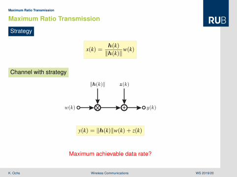
Maximum Ratio Transmission
Scenario
w(k) Tx
x1(k)
xm(k)
h1(k)
hm(k)
z(k)
y(k)Rx w(k)
feed-back channel
Transmitter has perfect channel state information (CSIT)
Channel
y(k) = hH(k)x(k) + z(k) , with Pz = σ2z
Lehrstuhl fürDigitale Kommunikationssysteme
K. Ochs Wireless Communications WS 2019/20
Maximum Ratio Transmission 90 / 126
Maximum Ratio Transmission
Strategy
x(k) =h(k)‖h(k)‖w(k)
Channel with strategy
w(k)
‖h(k)‖ z(k)
y(k)
y(k) = ‖h(k)‖w(k) + z(k)
Maximum achievable data rate?
Lehrstuhl fürDigitale Kommunikationssysteme
K. Ochs Wireless Communications WS 2019/20

Maximum Ratio Transmission 91 / 126
Maximum Ratio Transmission
Signal to noise ratio
γSNR = E|‖h‖w|2E|z|2 = ‖h‖2E|w|2
σ2z
=‖h‖2E
∥∥∥ h‖h‖ w
∥∥∥2
σ2z
=‖h‖2E‖x‖2
σ2z
= ‖h‖2ΓSNR
Achievable data rate
R(k) ≤ Rmax(k) = ld(
1 + ‖h(k)‖2ΓSNR
)Capacity of the (MIMO) channel
C(k) = ld(1 + hH(k)h(k)ΓSNR
)Performance of strategy
Rmax(k) = C(k)
Maximum ratio transmission is optimal!Lehrstuhl fürDigitale Kommunikationssysteme
K. Ochs Wireless Communications WS 2019/20

Optimal Transmission Strategies Water-Filling
Contents
1 Maximum Ratio Combining
2 Maximum Ratio Transmission
3 Water-Filling
Lehrstuhl fürDigitale Kommunikationssysteme
K. Ochs Wireless Communications WS 2019/20
Water-Filling 92 / 126
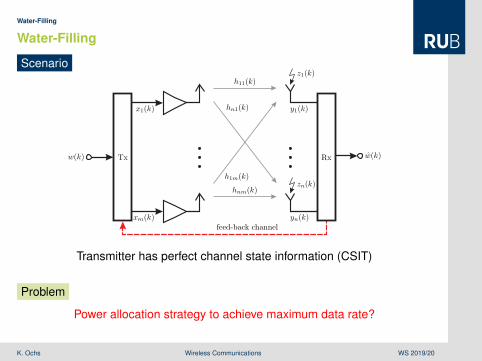
Water-Filling
Scenario
w(k)
x1(k)
xm(k)
h11(k)
hn1(k)
h1m(k)
hnm(k)
z1(k)
zn(k)
y1(k)
yn(k)
w(k)Tx Rx
feed-back channel
Transmitter has perfect channel state information (CSIT)
Problem
Power allocation strategy to achieve maximum data rate?
Lehrstuhl fürDigitale Kommunikationssysteme
K. Ochs Wireless Communications WS 2019/20

Water-Filling 93 / 126
Water-Filling
Prerequisite
CSIT allows for singular value decomposition
exploit SVD to reduce problem to parallel SISO channels
r = rank(H) , with H = UΣV H ,
noise power at each receiver antenna
Pz% = σ2z% for % = 1, . . . , r = rank(H)
variable transmit signal power
Px% = α%Px , with α% ≥ 0
limited total transmit power
E‖x(k)‖2 ≤ mPx , respectivelyr∑
%=1
Px% ≤ mPx
Lehrstuhl fürDigitale Kommunikationssysteme
K. Ochs Wireless Communications WS 2019/20
Water-Filling 94 / 126
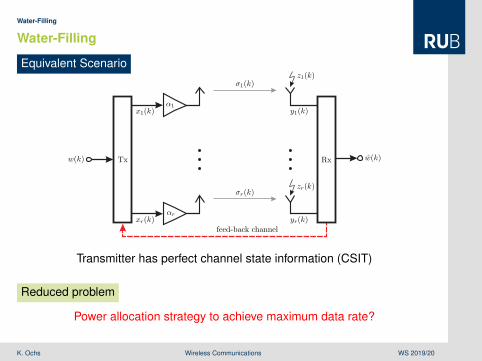
Water-Filling
Equivalent Scenario
w(k)
α1
αr
x1(k)
xr(k)
σ1(k)
σr(k)
z1(k)
zr(k)
y1(k)
yr(k)
w(k)Tx Rx
feed-back channel
Transmitter has perfect channel state information (CSIT)
Reduced problem
Power allocation strategy to achieve maximum data rate?Lehrstuhl fürDigitale Kommunikationssysteme
K. Ochs Wireless Communications WS 2019/20
Water-Filling 95 / 126
Water-Filling
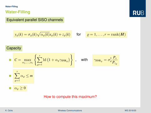
Equivalent parallel SISO channels
y%(k) = σ%(k)√α%(k)x%(k) + z%(k) for % = 1, . . . , r = rank(H)
Capacity
C = maxα1,...,αr
r∑
%=1
ld(1 + α%γSNR%
), with γSNR% = σ2
%Px
Pz%
r∑%=1
α% ≤ m
α% ≥ 0
How to compute this maximum?
Lehrstuhl fürDigitale Kommunikationssysteme
K. Ochs Wireless Communications WS 2019/20

Water-Filling 96 / 126
Water-Filling
Optimization problem formulation
minα f (α) s. t. g(α) ≤ 0 , α 0
Objective function
f (α) = −r∑
%=1
ld(1 + α%γSNR%
)differentiable, convex
Inequality constraint function
g(α) =r∑
%=1
α% − m
differentiable, convex
Convex optimization problem!Lehrstuhl fürDigitale Kommunikationssysteme
K. Ochs Wireless Communications WS 2019/20

Water-Filling 97 / 126
Water-Filling
Karush-Kuhn-Tucker conditions In particular , with % = 1, . . . , r
1 µ ≥ 0 1 µ = 0 or µ > 0
2 f ′(α) + µg′(α) = 0T 2 − γSNR%
ln(2)[1 + α%γSNR%
] + µ = 0
3 µg(α) = 0 3 µ
[r∑
%=1
α% − m
]= 0
4 g(α) ≤ 0 4
r∑%=1
α% − m ≤ 0
5 α ≥ 0 5 α% ≥ 0
For this convex optimization problem theKarush-Kuhn-Tucker conditions are necessary and sufficient!
Lehrstuhl fürDigitale Kommunikationssysteme
K. Ochs Wireless Communications WS 2019/20

Water-Filling 98 / 126
Water-Filling
Consequences
2 ⇒ µ =γSNR%
ln(2)[1 + α%γSNR%
] > 0
1 is feasible
3 ⇒r∑
%=1
α% = m
4 is feasible
2 ⇒ α% =1
µ ln(2)− 1γSNR%
Solution
5 ⇒ α% =
(1
µ ln(2)− 1γSNR%
)+
for % = 1, . . . , r
Lehrstuhl fürDigitale Kommunikationssysteme
K. Ochs Wireless Communications WS 2019/20

Water-Filling 99 / 126
Water-Filling
Water-Filling Algorithm γSNR1 ≥ γSNR2 ≥ · · · ≥ γSNRr > 0
1 2 3 4 • • • r − 1 r
1γSNR1
1γSNR2
1γSNR3
1µ ln(2)
1γSNR4
1γSNRr−1
1γSNRr
α1 α
2
α3
α4=0
αr−1=0
αr=0
•••
Who has will be given more!Lehrstuhl fürDigitale Kommunikationssysteme
K. Ochs Wireless Communications WS 2019/20

Wireless Communications Multiple Access Channel
Wireless CommunicationsMultiple Access Channel
Karlheinz Ochs
Chair of Digital Communication Systems
Lehrstuhl fürDigitale Kommunikationssysteme
K. Ochs Wireless Communications WS 2019/20
Multiple Access Channel
Contents
1 Scenario
2 Time Division Multiple Access
3 Time Sharing
4 Successive Interference Cancelation
Lehrstuhl fürDigitale Kommunikationssysteme
K. Ochs Wireless Communications WS 2019/20

Multiple Access Channel Scenario
Contents
1 Scenario
2 Time Division Multiple Access
3 Time Sharing
4 Successive Interference Cancelation
Lehrstuhl fürDigitale Kommunikationssysteme
K. Ochs Wireless Communications WS 2019/20

Scenario 100 / 126
Scenario
Scenario
w1(k)
w2(k)
Tx1
Tx2
x1(k)
x2(k)
h∗1
h∗2
z(k)
y(k)Rx w1(k), w2(k)
Transmitters have no channel state information (no CSIT)
Channel
y(k) = hHx(k) + z(k) , with Kxx = diag(Px1 ,Px2) , Pz = σ2z
Lehrstuhl fürDigitale Kommunikationssysteme
K. Ochs Wireless Communications WS 2019/20

Scenario 101 / 126
Scenario
Signal flow diagram
x1(k)
x2(k)
h∗1
h∗2
z(k)
y(k)
Channel
y(k) = h∗1 x1(k) + h∗2 x2(k) + z(k)
Objective
R1 + R2 → max
Optimal transmission strategy?
Lehrstuhl fürDigitale Kommunikationssysteme
K. Ochs Wireless Communications WS 2019/20
Multiple Access Channel Time Division Multiple Access
Contents
1 Scenario
2 Time Division Multiple Access
3 Time Sharing
4 Successive Interference Cancelation
Lehrstuhl fürDigitale Kommunikationssysteme
K. Ochs Wireless Communications WS 2019/20

Time Division Multiple Access 102 / 126
Time Division Multiple Access
Time Division Multiple Access Strategy
x1(k)
x2(k)
k ∈ K1
k ∈ K2
h∗1
h∗2
z(k)
y(k)
Transmitter Tx1
k ∈ K1 = 1, . . . ,κ
1K
κ∑k=1
P1 ≤ Px1
worst case κ = K, (K2 = ∅)P1 ≤ Px1
Transmitter Tx2
k ∈ K2 = κ + 1, . . . ,K
1K
K∑k=κ+1
P2 ≤ Px2
worst case κ = 0, (K1 = ∅)P2 ≤ Px2
Lehrstuhl fürDigitale Kommunikationssysteme
K. Ochs Wireless Communications WS 2019/20

Time Division Multiple Access 103 / 126
Time Division Multiple Access
Channel usage proportions
Tx1: α =κK Tx2: 1− α
Maximum achievable data rates
Tx1: R1 ≤ αC1 ,
with C1 = ld
(1 + |h1|2 Px1
σ2z
) Tx2: R2 ≤ [1− α]C2 ,
with C2 = ld
(1 + |h2|2 Px2
σ2z
)
Rate region
R2 ≤ C2 − C2
C1R1
Lehrstuhl fürDigitale Kommunikationssysteme
K. Ochs Wireless Communications WS 2019/20

Time Division Multiple Access 104 / 126
Time Division Multiple Access
TDMA Rate Region
0 C10
C2
TDMA
α = 0
α = 1
R1
R2
Optimal strategy?Lehrstuhl fürDigitale Kommunikationssysteme
K. Ochs Wireless Communications WS 2019/20

Multiple Access Channel Time Sharing
Contents
1 Scenario
2 Time Division Multiple Access
3 Time Sharing
4 Successive Interference Cancelation
Lehrstuhl fürDigitale Kommunikationssysteme
K. Ochs Wireless Communications WS 2019/20

Time Sharing 105 / 126
Time Sharing
Time Sharing Strategy
x1(k)
x2(k)
k ∈ K1
k ∈ K2
1√α
1√1−α
h∗1
h∗2
z(k)
y(k)
Transmitter Tx1
k ∈ K1 = 1, . . . ,κ
1K
κ∑k=1
P1 ≤ Px1
average power constraintαP1 ≤ Px1 , α 6= 0
Transmitter Tx2
k ∈ K2 = κ + 1, . . . ,K
1K
K∑k=κ+1
P2 ≤ Px2
average power constraint[1− α]P2 ≤ Px2 , α 6= 1
Lehrstuhl fürDigitale Kommunikationssysteme
K. Ochs Wireless Communications WS 2019/20
Time Sharing 106 / 126
Time Sharing
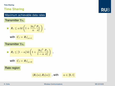
Maximum achievable data rates
Transmitter Tx1
R1 ≤ α ld
(1 +|h1|2α
Px1
σ2z
),
with C1 = R1|α=1
Transmitter Tx2
R2 ≤ [1− α] ld(
1 +|h2|2
1− αPx2
σ2z
),
with C2 = R2|α=0
Rate region
(R1(α),R2(α)) , with α ∈ [0, 1]
Lehrstuhl fürDigitale Kommunikationssysteme
K. Ochs Wireless Communications WS 2019/20

Time Sharing 107 / 126
Time Sharing
Time Sharing Rate Region
0 C10
C2
TDMA
Time-Sharing
α = 0
α = 1
R1
R2
Optimal strategy?Lehrstuhl fürDigitale Kommunikationssysteme
K. Ochs Wireless Communications WS 2019/20
Multiple Access Channel Successive Interference Cancelation
Contents
1 Scenario
2 Time Division Multiple Access
3 Time Sharing
4 Successive Interference Cancelation
Lehrstuhl fürDigitale Kommunikationssysteme
K. Ochs Wireless Communications WS 2019/20

Successive Interference Cancelation 108 / 126
Successive Interference Cancelation
Upper Bounds
1 Tx1 transmits only
R1 ≤ C1 , with C1 = ld
(1 + |h1|2 Px1
σ2z
)
2 Tx2 transmits only
R2 ≤ C2 , with C2 = ld
(1 + |h2|2 Px2
σ2z
)
3 Tx1, Tx2 are cooperating (MISO)
R2 ≤ −R1 + C , with C = ld
(1 + |h1|2 Px1
σ2z+ |h2|2 Px2
σ2z
)
Are the upper bounds achievable?
Lehrstuhl fürDigitale Kommunikationssysteme
K. Ochs Wireless Communications WS 2019/20

Successive Interference Cancelation 109 / 126
Successive Interference Cancelation
Successive Interference Cancelation Rate Region
0 R12 C10
R21
C2Tx2 transmits only
Tx1 , Tx
2 are cooperating
Tx1
transmits
only
R1
R2
Upper bounds achievable?
Lehrstuhl fürDigitale Kommunikationssysteme
K. Ochs Wireless Communications WS 2019/20

Successive Interference Cancelation 109 / 126
Successive Interference Cancelation
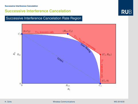
Successive Interference Cancelation Rate Region
0 R12 C10
R21
C2Tx2 transmits only
Tx1 , Tx
2 are cooperating
Tx1
transmits
only
TDMA
Time-Sharing
(0, C2)
(C1, 0)
(R12, C2)
(C1, R21)
R1
R2
Upper bounds achievable?Lehrstuhl fürDigitale Kommunikationssysteme
K. Ochs Wireless Communications WS 2019/20

Successive Interference Cancelation 110 / 126
Successive Interference Cancelation
Known upper bound
3 R1 ≤ ld
(1 + |h1|2 Px1
σ2z+ |h2|2 Px2
σ2z
)− R2
Achievability
(R1,R2) = (R12,C2)
Lehrstuhl fürDigitale Kommunikationssysteme
K. Ochs Wireless Communications WS 2019/20

Successive Interference Cancelation 110 / 126
Successive Interference Cancelation
Known upper bound
3 R1 ≤ ld
(1 + |h1|2 Px1
σ2z+ |h2|2 Px2
σ2z
)− R2
Achievability
(R1,R2) = (R12,C2)
R12 ≤ ld
(1 + |h2|2 Px2
σ2z+ |h1|2 Px1
σ2z
)− ld
(1 + |h2|2 Px2
σ2z
)
Lehrstuhl fürDigitale Kommunikationssysteme
K. Ochs Wireless Communications WS 2019/20

Successive Interference Cancelation 110 / 126
Successive Interference Cancelation
Known upper bound
3 R1 ≤ ld
(1 + |h1|2 Px1
σ2z+ |h2|2 Px2
σ2z
)− R2
Achievability
(R1,R2) = (R12,C2)
R12 ≤ ld
(1 +
|h1|2Px1
σ2z + |h2|2Px2
)
Successive interference cancelation strategy
1 receiver decodes x1 treating x2 as noise : R1 = R12
2 receiver cancels x1 by decoding x2 from y− h∗1 x1 : R2 = C2
Point (R12,C2) is achievable!Lehrstuhl fürDigitale Kommunikationssysteme
K. Ochs Wireless Communications WS 2019/20
Successive Interference Cancelation 111 / 126
Successive Interference Cancelation
Successive Interference Cancelation Rate Region
0 R12 C10
R21
C2Tx2 transmits only
Tx1 , Tx
2 are cooperating
Tx1
transmits
only
TDMA
Time-Sharing
(0, C2)
(C1, 0)
(R12, C2)
(C1, R21)
R1
R2
Lehrstuhl fürDigitale Kommunikationssysteme
K. Ochs Wireless Communications WS 2019/20

Successive Interference Cancelation 112 / 126
Successive Interference Cancelation
Known upper bound
3 R2 ≤ ld
(1 + |h1|2 Px1
σ2z+ |h2|2 Px2
σ2z
)− R1
Achievability
(R1,R2) = (C1,R21)
R21 ≤ ld
(1 +
|h2|2Px2
σ2z + |h1|2Px1
)
Successive interference cancelation strategy
1 receiver decodes x2 treating x1 as noise : R2 = R21
2 receiver cancels x2 by decoding x1 from y− h∗2 x2 : R1 = C1
Point (C1,R21) is achievable!Lehrstuhl fürDigitale Kommunikationssysteme
K. Ochs Wireless Communications WS 2019/20

Successive Interference Cancelation 113 / 126
Successive Interference Cancelation
Successive Interference Cancelation Rate Region
0 R12 C10
R21
C2Tx2 transmits only
Tx1 , Tx
2 are cooperating
Tx1
transmits
only
TDMA
Time-Sharing
(0, C2)
(C1, 0)
(R12, C2)
(C1, R21)
R1
R2
Lehrstuhl fürDigitale Kommunikationssysteme
K. Ochs Wireless Communications WS 2019/20

Successive Interference Cancelation 114 / 126
Successive Interference Cancelation
Achievable Points
1 Tx1 transmits only
(R1,R2) = (C1, 0)
2 Tx2 transmits only
(R1,R2) = (0,C2)
3 receiver successively cancels interference
(R1,R2) = (R12,C2)
4 receiver successively cancels interference
(R1,R2) = (C1,R21)
Use TDMA of the particular strategiesto achieve points on the connecting line!
Lehrstuhl fürDigitale Kommunikationssysteme
K. Ochs Wireless Communications WS 2019/20

Successive Interference Cancelation 115 / 126
Successive Interference Cancelation
Successive Interference Cancelation Rate Region
0 R12 C10
R21
C2
TDMA
Time-Sharing
(0, C2)
(C1, 0)
(R12, C2)
(C1, R21)
R1
R2
Successive interference cancelation is an optimal strategy!Lehrstuhl fürDigitale Kommunikationssysteme
K. Ochs Wireless Communications WS 2019/20

Wireless Communications X Channel
Wireless CommunicationsX Channel
Karlheinz Ochs
Chair of Digital Communication Systems
Lehrstuhl fürDigitale Kommunikationssysteme
K. Ochs Wireless Communications WS 2019/20

X Channel
Contents
1 Transmission Scenario
2 Interference Alignment
3 Interference Cancelation
Lehrstuhl fürDigitale Kommunikationssysteme
K. Ochs Wireless Communications WS 2019/20

X Channel Transmission Scenario
Contents
1 Transmission Scenario
2 Interference Alignment
3 Interference Cancelation
Lehrstuhl fürDigitale Kommunikationssysteme
K. Ochs Wireless Communications WS 2019/20

Transmission Scenario 116 / 126
X Channel
Transmission Scenario
u(t) h(t, t′) v(t)
Requirement specifications
k even [v1(kT)v2(kT)
]=
[u1(kT)u2(kT)
]
k odd [v1(kT)v2(kT)
]=
[u2(kT)u1(kT)
]
Lehrstuhl fürDigitale Kommunikationssysteme
K. Ochs Wireless Communications WS 2019/20

Transmission Scenario 116 / 126
X Channel
Transmission Scenario
u(t) h(t, t′) v(t)
Requirement specifications
k even [v1(kT)v2(kT)
]=
[u1(kT)u2(kT)
]or H(kT, jω′) =
[1 00 1
]
k odd [v1(kT)v2(kT)
]=
[u2(kT)u1(kT)
]or H(kT, jω′) =
[0 11 0
]
Lehrstuhl fürDigitale Kommunikationssysteme
K. Ochs Wireless Communications WS 2019/20

Transmission Scenario 116 / 126
X Channel
Transmission Scenario
u(t) h(t, t′) v(t) u(t) Encoderx(t)
Channely(t)
Decoder v(t)
Requirement specifications
k even [v1(kT)v2(kT)
]=
[u1(kT)u2(kT)
]or H(kT, jω′) =
[1 00 1
]
k odd [v1(kT)v2(kT)
]=
[u2(kT)u1(kT)
]or H(kT, jω′) =
[0 11 0
]
Optimal usage of channel resources?
Lehrstuhl fürDigitale Kommunikationssysteme
K. Ochs Wireless Communications WS 2019/20
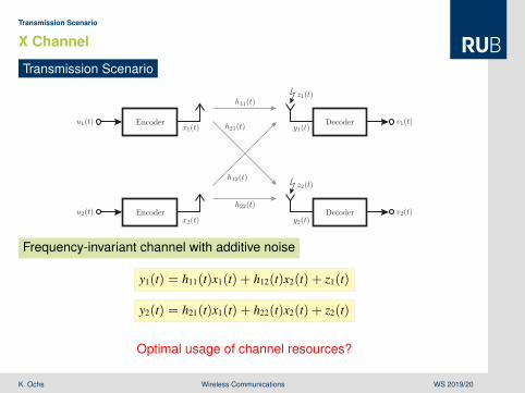
Transmission Scenario 117 / 126
X Channel
Transmission Scenario
u1(t)
u2(t)
x1(t)
x2(t)
h11(t)
h21(t)
h12(t)
h22(t)
z1(t)
z2(t)
y1(t)
y2(t)
v1(t)
v2(t)Encoder
Encoder
Decoder
Decoder
Frequency-invariant channel with additive noise
y1(t) = h11(t)x1(t) + h12(t)x2(t) + z1(t)
y2(t) = h21(t)x1(t) + h22(t)x2(t) + z2(t)
Optimal usage of channel resources?Lehrstuhl fürDigitale Kommunikationssysteme
K. Ochs Wireless Communications WS 2019/20

Transmission Scenario 118 / 126
X Channel
Simplified Transmission Scenario
u11, u21
u22, u12
x1(k)
x2(k)
h11(k)
h21(k)
h12(k)
h22(k)
y1(k)
y2(k)
u11, u12
u22, u21Encoder
Encoder
Decoder
Decoder
Frequency-invariant channel
y1(k) = h11(k)x1(k) + h12(k)x2(k)
y2(k) = h21(k)x1(k) + h22(k)x2(k)
Transmission of 4 symbols with 3 channel usages?Lehrstuhl fürDigitale Kommunikationssysteme
K. Ochs Wireless Communications WS 2019/20
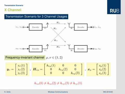
Transmission Scenario 119 / 126
X Channel
Transmission Scenario for 3 Channel Usages
u11, u21
u22, u12
x1
x2
H11
H21
H12
H22
y1
y2
u11, u12
u22, u21Encoder
Encoder
Decoder
Decoder
Frequency-invariant channel µ, ν ∈ 1, 2
yν =
yν(1)yν(2)yν(3)
, Hνµ =
hνµ(1) 0 00 hνµ(2) 00 0 hνµ(3)
, xµ =
xµ(1)xµ(2)xµ(3)
hνµ(1) 6= hνµ(2) 6= hνµ(3) 6= hνµ(1)Lehrstuhl fürDigitale Kommunikationssysteme
K. Ochs Wireless Communications WS 2019/20

X Channel Interference Alignment
Contents
1 Transmission Scenario
2 Interference Alignment
3 Interference Cancelation
Lehrstuhl fürDigitale Kommunikationssysteme
K. Ochs Wireless Communications WS 2019/20

Interference Alignment 120 / 126
X Channel
Transmission Scenario for 3 Channel Usages
u11, u21
u22, u12
x1
x2
H11
H21
H12
H22
y1
y2
u11, u12
u22, u21Encoder
Encoder
Decoder
Decoder
Transmitted signals
x1 = q11u11 + q21u21
x2 = q12u12 + q22u22
Vectors qνµ are design parameters!Lehrstuhl fürDigitale Kommunikationssysteme
K. Ochs Wireless Communications WS 2019/20
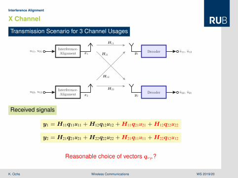
Interference Alignment 121 / 126
X Channel
Transmission Scenario for 3 Channel Usages
u11, u21
u22, u12
x1
x2
H11
H21
H12
H22
y1
y2
u11, u12
u22, u21Interference-Alignment
Interference-Alignment
Decoder
Decoder
Received signals
y1 =H11q11u11 +H12q12u12 +H11q21u21 +H12q22u22
y2 =H21q21u21 +H22q22u22 +H21q11u11 +H22q12u12
Reasonable choice of vectors qνµ?Lehrstuhl fürDigitale Kommunikationssysteme
K. Ochs Wireless Communications WS 2019/20
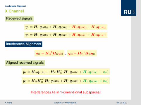
Interference Alignment 122 / 126
X Channel
Received signals
y1 =H11q11u11 +H12q12u12 +H11q21u21 +H12q22u22
y2 =H21q21u21 +H22q22u22 +H21q11u11 +H22q12u12
Interference Alignment
q21 =H−111 H12q22 , q12 =H−1
22 H21q11
Aligned received signals
y1 =H11q11u11 +H12H−122 H21q11u12 +H12q22[u21 + u22]
y2 =H21H−111 H12q22u21 +H22q22u22 +H21q11[u11 + u12]
Interferences lie in 1-dimensional subspaces!Lehrstuhl fürDigitale Kommunikationssysteme
K. Ochs Wireless Communications WS 2019/20

X Channel Interference Cancelation
Contents
1 Transmission Scenario
2 Interference Alignment
3 Interference Cancelation
Lehrstuhl fürDigitale Kommunikationssysteme
K. Ochs Wireless Communications WS 2019/20

Interference Cancelation 123 / 126
X Channel
Transmission Scenario for 3 Channel Usages
u11, u21
u22, u12
x1
x2
H11
H21
H12
H22
y1
y2
u11, u12
u22, u21Interference-Alignment
Interference-Alignment
Decoder
Decoder
Aligned received signals
y1 =H11q11u11 +H12H−122 H21q11u12 +H12q22[u21 + u22]
y2 =H21H−111 H12q22u21 +H22q22u22 +H21q11[u11 + u12]
Choice of q11 and q22, such that decoding is possible?Lehrstuhl fürDigitale Kommunikationssysteme
K. Ochs Wireless Communications WS 2019/20

Interference Cancelation 124 / 126
X Channel
Aligned received signals
y1 = R1
u11
u12
u21 + u22
and y2 = R2
u21
u22
u11 + u12
with matrices depending on vectors q11 and q22
R1 =[H11q11 H12H
−122 H21q11 H12q22
]R2 =
[H21H
−111 H12q22 H22q22 H21q11
]Decoding of transmitted symbols
Choice of q11 and q22, such that R1 and R2 are regular?
Lehrstuhl fürDigitale Kommunikationssysteme
K. Ochs Wireless Communications WS 2019/20

Interference Cancelation 125 / 126
X Channel
Transmission Scenario for 3 Channel Usages
u11, u21
u22, u12
x1
x2
H11
H21
H12
H22
y1
y2
u11, u12
u22, u21Interference-Alignment
Interference-Alignment
Decoder
Decoder
Interference Cancelation u11
u12
u21 + u22
= R−11 y1 and
u22
u21
u11 + u12
= R−12 y2
Lehrstuhl fürDigitale Kommunikationssysteme
K. Ochs Wireless Communications WS 2019/20

Interference Cancelation 126 / 126
X Channel
Transmission Scenario for 3 Channel Usages
u(t) Encoderx(t)
Channely(t)
Decoder v(t)
Remarks
encoder and decoder are time-variant transmission systems
channel state information at transmitter required
transmission of 4 symbols with 3 channel uses
strategy achieves DoF
DoF is a first order approximation of channel capacity
Information theory
Interference alignment and cancelation is a DoF-optimal strategy!
Lehrstuhl fürDigitale Kommunikationssysteme
K. Ochs Wireless Communications WS 2019/20