Session2 Antennas and Propagation

Wireless Communication

Presented by

Dr. Mahmoud Daneshvar

1

1. Introduction• Types of Anttenas• Free space Propagation

2. Propagation modes3. Transmission Problems4. Fading

1. Introduction

An antenna is an electrical conductor or system of conductors Transmission - radiates electromagnetic

energy into space

Reception - collects electromagnetic energy from space

In two-way communication, the same antenna can be used for transmission and reception

2

Radiation Patterns

Radiation pattern

Graphical representation of radiation properties of an antenna

Depicted as two-dimensional cross section

Beam width (or half-power beam width)

Measure of directivity of antenna

Reception pattern

Receiving antenna’s equivalent to radiation pattern

3

Types of Antennas

Isotropic antenna (idealized) Radiates power equally in all directions

Dipole antennas Half-wave dipole antenna (or Hertz

antenna)

Quarter-wave vertical antenna (or Marconi antenna)

Parabolic Reflective Antenna

4

5

6

7

8

Antenna Gain Antenna gain

Measure of the directionality of an antenna

Power output, in a particular direction, compared to that produced in any direction by a perfect omnidirectional antenna (isotropic antenna)

Effective area

Related to physical size and shape of antenna

9

Free-space propagation

10

)d

Omni-directional transmitting antenna Receiving antenna, area AR

where is an efficiency parameter

Transmitted power PT

Received power PR

Focusing capability: determined by the antenna size in wavelenths (the wavelength is λ):

where is the transmitting antenna efficiency factor

Directional antenna

11

)d

Transmitting antenna, area AT Receiving antenna, area AR

Transmitted power PT Received power PR

Directional antenna gain GT > 1

(

Similarly to what done on previous slide:

Hence: free-space received power:

2. Propagation Modes

Ground-wave propagation

Sky-wave propagation

Line-of-sight propagation

12

13

Ground Wave Propagation

14

Ground Wave Propagation

Follows contour of the earth

The electromagnetic wave induces a current in hte earth’s surface the waveform tilts downwards

Diffraction

Can Propagate considerable distances

Frequencies up to 2 MHz

Example

AM radio15

Sky Wave Propagation

16

Sky Wave Propagation

Signal reflected from ionized layer of atmosphere back down to earth

Signal can travel a number of hops, back and forth between ionosphere and earth’s surface

Reflection effect caused by refraction

Examples

Amateur radio

CB radio

17

Line-of-Sight Propagation

18

Line-of-Sight Propagation Required above 30 MHz

Transmitting and receiving antennas must be within line of sight Satellite communication – signal above 30 MHz

not reflected by ionosphere

Ground communication – antennas within effectiveline of site due to refraction

Refraction – bending of microwaves by the atmosphere Velocity of electromagnetic wave is a function of

the density of the medium

When wave changes medium, speed changes

Wave bends at the boundary between mediums

19

20

Line-of-Sight Equations

Optical line of sight

Effective, or radio, line of sight

d = distance between antenna and horizon (km)

h = antenna height (m)

K = adjustment factor to account for refraction, rule of thumb K = 4/3

hd 57.3

hd 57.3

21

Line-of-Sight Equations

Maximum distance between two antennas for LOS propagation:

h1 = height of antenna one

h2 = height of antenna two

2157.3 hh

22

3. Transmission problems

Attenuation

Free space loss

attenuation distortion

Noise

Atmospheric absorption

Multipath

Refraction

23

Attenuation

Strength of signal falls off with distance over transmission medium

Attenuation factors for unguided media: Received signal must have sufficient strength so

that circuitry in the receiver can interpret the signal

Signal must maintain a level sufficiently higher than noise to be received without error

Attenuation is greater at higher frequencies, causing distortion

24

Free Space Loss

Free space loss, ideal isotropic antenna

Pt = signal power at transmitting antenna

Pr = signal power at receiving antenna

l = carrier wavelength

d = propagation distance between antennas

c = speed of light 3 10 8 m/s)

where d and l are in the same units (e.g., meters)

2

2

2

244

c

fdd

P

P

r

t

l

25

Free Space Loss

Free space loss equation can be recast:

l

d

P

PL

r

tdB

4log20log10

dB 98.21log20log20 dl

dB 56.147log20log204

log20

df

c

fd

26

27

Free Space Loss

Free space loss accounting for gain of other kinds of antennas

Gt = gain of transmitting antenna

Gr = gain of receiving antenna

At = effective area of transmitting antenna

Ar = effective area of receiving antenna

trtrtrr

t

AAf

cd

AA

d

GG

d

P

P2

22

2

224

l

l

28

Free Space Loss

Free space loss accounting for gain of other kinds of antennas can be recast as

rtdB AAdL log10log20log20 l

dB54.169log10log20log20 rt AAdf

29

Categories of Noise

Thermal Noise

Intermodulation noise

Crosstalk

Impulse Noise

30

Thermal Noise

Also called white noise

Due to agitation of electrons

Present in all electronic devices and transmission media

Cannot be eliminated

Function of temperature

Particularly significant for satellite communication

31

Thermal Noise

Amount of thermal noise to be found in a bandwidth of 1Hz in any device or conductor is:

N0 = noise power density in watts per 1 Hz of bandwidth

k = Boltzmann's constant = 1.3803 10-23 J/K

T = temperature, in kelvins (absolute temperature)

W/Hz k0 TN

32

Thermal Noise

Noise is assumed to be independent of frequency

Thermal noise present in a bandwidth of BHertz (in watts):

or, in decibel-watts

TBN k

BTN log10 log 10k log10

BT log10 log 10dBW 6.228 33

Noise Terminology

Intermodulation noise – occurs if signals with different frequencies share the same medium Interference caused by a signal produced at a

frequency that is the sum or difference of original frequencies

Crosstalk – unwanted coupling between signal paths

Impulse noise – irregular pulses or noise spikes Short duration and of relatively high amplitude

Caused by external electromagnetic disturbances, or faults and flaws in the communications system

34

Expression Eb/N0

Ratio of signal energy per bit to noise power density per Hertz

where S is the signal power, R the bitrate, kBoltzmann’s constant and T the temperature

The bit error rate for digital data is a function of Eb/N0

Given a value for Eb/N0 to achieve a desired error rate, parameters of this formula can be selected

As bit rate R increases, transmitted signal power must increase to maintain required Eb/N0

TR

S

N

RS

N

Ebk

/

00

35

36

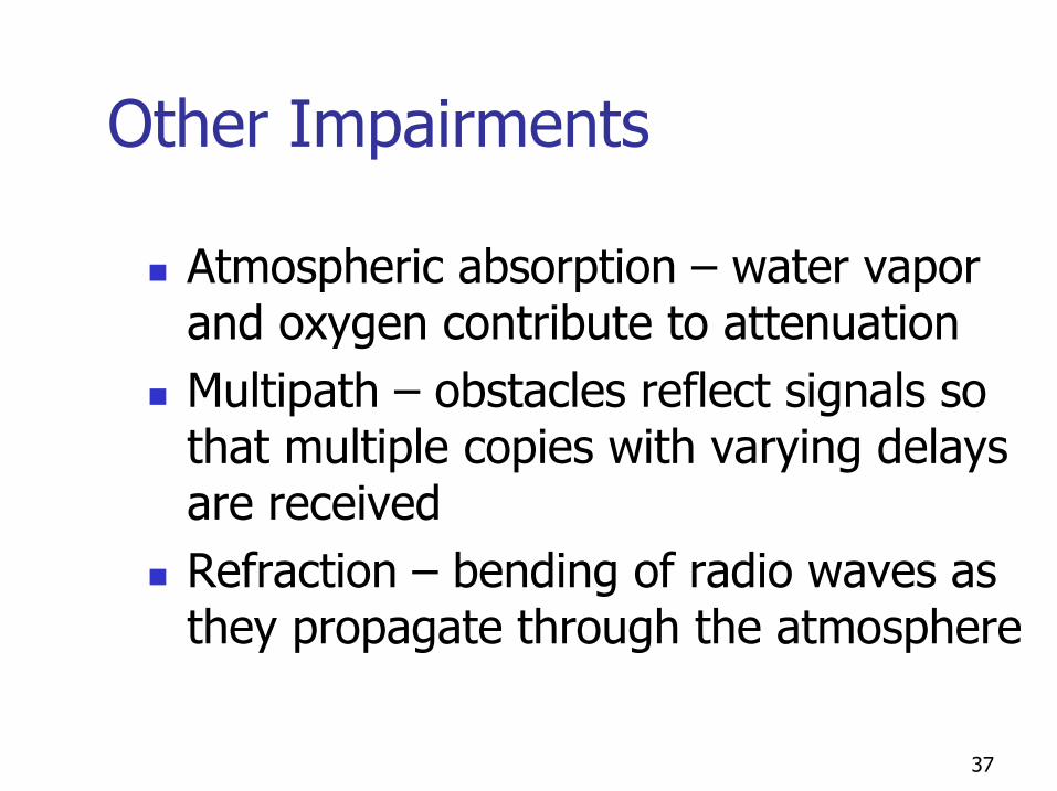
Other Impairments

Atmospheric absorption – water vapor and oxygen contribute to attenuation

Multipath – obstacles reflect signals so that multiple copies with varying delays are received

Refraction – bending of radio waves as they propagate through the atmosphere

37

4. FadingFading: time variation of received signal power due to

changes in the transmission medium or path(s)

Kinds of fading:

Fast fading

Slow fading

Flat fading independent from frequency

Selective fading frequency-dependent

Rayleigh fading no dominant path

Rician fading Line Of Sight (LOS) is dominating + presence of indirect multipath signals

38

39

Multipath Propagation

Reflection - occurs when signal encounters a surface that is large relative to the wavelength of the signal

Diffraction - occurs at the edge of an impenetrable body that is large compared to wavelength of radio wave

Scattering – occurs when incoming signal hits an object whose size in the order of the wavelength of the signal or less

40

Multipath Propagation

41

The Effects of Multipath Propagation

Multiple copies of a signal may arrive at different phases If phases add destructively, the signal level

relative to noise declines, making detection more difficult

Intersymbol interference (ISI) One or more delayed copies of a pulse may

arrive at the same time as the primary pulse for a subsequent bit

42

Propagation Characteristics

Path Loss (includes average shadowing)

Shadowing (due to obstructions)

Multipath Fading

Pr/Pt

d=vt

PrPt

d=vt

v Very slow

SlowFast

Path Loss Modeling

Maxwell’s equations Complex and impractical

Free space path loss model Too simple

Ray tracing models Requires site-specific information

Empirical Models Don’t always generalize to other environments

Simplified power falloff models Main characteristics: good for high-level analysis

Free Space (LOS) Model

Path loss for unobstructed LOS path

Power falls off :

Proportional to d2

Proportional to l2 (inversely proportional to f2)

d=vt

Ray Tracing Approximation

Represent wavefronts as simple particles

Geometry determines received signal from each signal component

Typically includes reflected rays, can also include scattered and defracted rays.

Requires site parameters

Geometry

Dielectric properties

Two Path Model

Path loss for one LOS path and 1 ground (or reflected) bounce

Ground bounce approximately cancels LOS path above critical distance

Power falls off

Proportional to d2 (small d)

Proportional to d4 (d>dc)

Independent of l (f)

General Ray Tracing

Models all signal components

Reflections

Scattering

Diffraction

Requires detailed geometry and dielectric properties of site Similar to Maxwell, but easier math.

Computer packages often used

Simplified Path Loss Model

82,0

g

g

d

dKPP tr

Used when path loss dominated by reflections.

Most important parameter is the path loss exponent g, determined empirically.

Empirical Models Okumura model

Empirically based (site/freq specific)

Awkward (uses graphs)

Hata model Analytical approximation to Okumura model

Cost 136 Model: Extends Hata model to higher frequency (2 GHz)

Walfish/Bertoni:

Cost 136 extension to include diffraction from rooftops

Commonly used in cellular system simulations

Main Points

Path loss models simplify Maxwell’s equations

Models vary in complexity and accuracy

Power falloff with distance is proportional to d2 in free space, d4 in two path model

General ray tracing computationally complex

Empirical models used in 2G simulations

Main characteristics of path loss captured in

simple model Pr=PtK[d0/d]g

52

53

54

Power in the dominant path

Power in the scattered pathsK

K=0 : RayleighK=∞: Additive White

Gaussian Noise

Solution

Error Compensation Mechanisms

Adaptive Equalization

Diversity Techniques

55

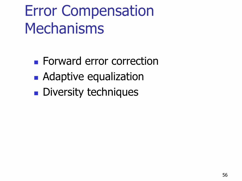
Error Compensation Mechanisms

Forward error correction

Adaptive equalization

Diversity techniques

56

Forward Error Correction

Transmitter adds error-correcting code to data block

Code is a function of the data bits

Receiver calculates error-correcting code from incoming data bits

If calculated code matches incoming code, no error occurred

If error-correcting codes don’t match, receiver attempts to determine bits in error and correct

57

Adaptive Equalization

Can be applied to transmissions that carry analog or digital information Analog voice or video

Digital data, digitized voice or video

Used to combat intersymbol interference

Involves gathering dispersed symbol energy back into its original time interval

Techniques Lumped analog circuits

Sophisticated digital signal processing algorithms

58

59

A known training sequence is sent periodically. The receiverfine tunes the coefficients accordingly.

Diversity Techniques

Diversity is based on the fact that individual channels experience independent fading events

Space diversity – techniques involving physical transmission path (e.g., multiple antennas)

Frequency diversity – techniques where the signal is spread out over a larger frequency bandwidth or carried on multiple frequency carriers

Time diversity – techniques aimed at spreading the data out over time

60

61