Winning by Losing: Evidence on the Long-Run E …moretti/mergers.pdfWinning by Losing: Evidence on...

Winning by Losing:

Evidence on the Long-Run Effects of Mergers∗

Ulrike Malmendier

UC Berkeley

NBER

Enrico Moretti

UC Berkeley

NBER

Florian Peters

University of

Amsterdam

Abstract

We propose a novel approach to measuring returns to mergers. In a new data set of closebidding contests we use losers’ post-merger performance to construct the counterfactualperformance of winners had they not won the contest. Stock returns of winners andlosers closely track each other over the 36 months before the merger, corroboratingour approach to identification. Bidders are also very similar in terms of Tobins Q,profitability and other accounting measures. Over the three years after the merger,however, losers outperform winners by 24 percent. Commonly used methodologiessuch as announcement returns fail to identify acquirors’ underperformance. (JEL G34,G14, D03)

∗ Ulrike Malmendier: UC Berkeley and NBER. Enrico Moretti: UC Berkeley and NBER. Florian Peters:University of Amsterdam. We thank Jeff Zeidel and seminar participants at Amsterdam, Chicago Booth,DePaul, LSE, Luxembourg School of Finance, MIT, NYU, Ohio State University, Princeton, TinbergenInstitute, Yale, and at the AFA, EFA, FIRS, and the NBER Summer Institute for valuable comments.We thank Zach Liscow and Jonas Sobott for excellent research assistance. Send correspondence to UlrikeMalmendier, UC Berkeley and NBER, 530 Evans Hall #3880, Berkeley, CA 94720-3880, USA; telephone:(510) 642-5038; email: [email protected].

Do acquiring companies profit from acquisitions, or do acquirors overbid and destroy share-

holder value? The negative stock-market reactions to a large number of merger announce-

ments (see, e.g., Moeller, Schlingemann, and Stulz (2005)) have attracted considerable at-

tention to this question. Researchers have interpreted such negative stock-price responses as

evidence of incentive misalignment (e.g., empire building) or behavioral biases (e.g., CEO

overconfidence).1

A major obstacle in the evaluation of mergers is that it is difficult to obtain unbiased

estimates of the value they create or destroy. The most common approach, announcement

returns, may be biased due to price pressure around mergers, information revealed in the

merger bid, or market inefficiencies.2 Another approach, the computation of long-run ab-

normal returns, may be biased due to unobserved differences between the firms that merge

and the firms that do not.3 For example, a decline in the acquiror’s market valuation after

a merger might not be caused by the merger, but could reflect, instead, that highly valued

firms choose to acquire less highly valued targets. In this case, the subsequent decline would

have occurred even in the absence of the takeover.4 It is difficult to find a valid control group

to whom we can compare acquiring firms, as the latter are a selected group and engage in

mergers at selected points in time.

In this paper, we propose a novel way to address these selection issues. We exploit merger

contests to evaluate the long-run effects of mergers on acquiror returns. The basic idea is to

use the returns to losing bidders to calculate the counterfactual performance of the matched

winners had they not won the contest. Participation in a bidding contest provides a novel

matching criterion, over and above the usual market-, industry-, and firm-level observables.

1 Jensen (1986), (Morck, Shleifer, and Vishny (1990)), (Roll (1986); Malmendier and Tate (2008)).2 See, for example, Mitchell, Pulvino, and Stafford (2004) and Asquith, Bruner, and Mullins Jr (1987).3 Loughran and Vijh (1997) and Rau and Vermaelen (1998).4 See the argument in Shleifer and Vishny (2003) and Rhodes-Kropf and Viswanathan (2004), as well as

the empirical tests in Dong, Hirshleifer, Richardson, and Teoh (2006), Savor and Lu (2009), and Rhodes-Kropf, Robinson, and Viswanathan (2005).

1

This approach offers an improvement over existing analyses to the extent that winners are

more similar to losers than to the average firm in the market or other previously used control

groups. It can account for strategic considerations that lead firms to attempt a specific

takeover at a specific point in time but that are hard to control for with the standard set of

financial variables. For example, the contest setting alleviates the concern about acquirors’

prior overvaluation since highly-valued winners are benchmarked against similarly-valued

losers.

An attractive feature of our approach is that we can probe the validity of our identifying

assumption by comparing the valuation paths of winners and losers in the months and years

prior to the merger contest. Any differences in expected performance between matched

winners and losers should materialize in diverging price paths before the merger. Stock prices

are particularly suitable for probing the validity of our identifying assumption because stock

valuations are forward looking and capture pre-merger market expectations about future

profitability. Another advantage of our approach is that it allows for all parties to re-

optimize after the merger, e.g., for the loser to acquire another target. In contrast to some of

the previous studies, our approach does not condition on endogeneous post-merger choices.

A disadvantage of our approach is that it is restricted to merger contests. We cannot

speak to the value generated in a broader set of mergers. In fact, the more we restrict the

sample for the sake of identification (e.g., not only to contested mergers, but to “close” cases

of contested mergers, as we will discuss below), the more we reduce generalizability. At the

same time, the methodological implications of our findings go beyond the sample of contests.

By comparing our estimates to estimates based on existing methodologies, both calculated

in our sample, we provide evidence on the biases embedded in other approaches and their

potential magnitude.

We collect data on all U.S. mergers with concurrent bids of at least two potential acquirors

2

since 1985. We validate the accuracy of the Thomson data regarding the contested nature

of the mergers using press reports.5 We also collect a similar international data set.

To maximize the similarity between winning and losing bidders, we exclude contests where

the initial bidder withdraws shortly after the competing bid arrives. Such short contests tend

to feature one bidder who is ex ante particularly likely to win, invalidating the identifying

assumption. Instead, we focus on protracted contests where bidders actively compete, for

example by making multiple offers and counter-offers. In such cases, all bidders tend to have

a significant ex-ante chance of winning the contest, ameliorating concerns about endogeneity

in the ultimate outcome.

We find that winners’ and losers’ have generally similar observable characteristics before

the merger, and are more similar than winners are to the average U.S. firm. In particular,

winners and losers are comparable in terms of pre-merger Tobin’s Q, PP&E, profitability,

book leverage, and market leverage. Most importantly, winners and losers display very

similar stock-market performance in the months leading up to the announcement, in par-

ticular in closely contested cases: Their buy-and-hold abnormal returns closely track each

other during the 36 months before the merger announcement, in particular in the sample

of protracted merger contests. In addition, analyst forecasts of winners’ and losers’ future

earnings-to-price ratios are similar. Thus, consistent with our identifying assumption, both

the market overall and experts evaluating the companies have similar expectations about

the future profitability of winners and losers before the merger.

After the merger, however, losers significantly outperform winners. The estimated effect

for U.S. mergers is economically large, a 23.3 to 33.2 percent difference in buy-and-hold

abnormal returns over the next three years relative to winners, depending on the sample and

type of abnormal return calculation. These differences in post-merger performance cannot

5 We search for press mentions in the Financial Times, Wall Street Journal, and Washington Post andin some models we require that at least one article mentions the competing bids identified by Thomson.

3

be attributed to changes in the risk profile of winners relative to losers since the results are

unaffected when we adjust for changes in risk exposure. We also show that they are not

explained by pre-merger run-ups in stock price or valuation differences in terms of market-

to-book ratio.

Outside the U.S. contested mergers generate less underperformance. We estimate a

statistically significant effect of 13.6 percent in the international sample.

While our main goal is to estimate the average effect of mergers, in the second part of

the paper we explore potential channels that may explain a negative effect. We focus on

three potential mechanisms that are commonly discussed in the literature: merger-induced

reductions in strategic flexibility, the post-merger cost of integration, and pre-existing target

inefficiencies. These mechanisms are of course not necessarily mutually exclusive.

We find that the loss of strategic and financial flexibility may help to explain the under-

performance of acquirors. The negative merger effect is estimated to be particularly large

in acquirors who spend their cash or bump up their leverage to finance the merger. We also

find that proxies for high costs of post-merger integration, based on industry differences or

relative acquiror/target size, predict larger than average effects. Finally, stock-based, cash-

flow based, and Q-based proxies point to the possibility that pre-existing target inefficiencies

may also play a role.

Thus, all three channels may help to explain the underperformance of acquirors. We

stress, however, that the estimation of these models is significantly more demanding than

the estimation of our baseline models as it requires us to subsample along the dimension of

the respective characteristic. As such these analyses yield estimates that are necessarily less

precise and should be considered suggestive, rather than definitive.

In the last part of the paper, we use our empirical approach to evaluate the main exist-

ing methods that have been employed to measure returns to mergers. When we calculate

announcement effects, alphas based on four-factor calendar-time regressions of winner-only

4

portfolios, and winners’ long-run buy-and-hold abnormal returns in our sample, we find

that none of these approaches capture the negative long-run return implications of contested

mergers. Winners’ announcement returns are insignificantly negative, both at the initial bid

and at the losing bidder’s withdrawal, and winners’ four-factor alphas as well as winners’

long-run buy-and-hold abnormal returns are insignificantly positive. Moreover, winners’ an-

nouncement returns display an insignificantly negative correlation with our estimates, i.e.,

fail to predict the causal effect of contested mergers even directionally.

This paper relates to a large literature estimating the value created in corporate takeovers,

which goes back at least to the 1970s (e.g., Mandelker (1974) and Dodd and Ruback (1977)).

Early reviews of the empirical evidence include Jensen and Ruback (1983) and Roll (1986);

more reviews are from Andrade, Mitchell, and Stafford (2001) and Betton, Eckbo, and Thor-

burn (2008). The assessment of the value effects of mergers has changed over the decades,

not only due to time variation in the data but also due to new methodology and economet-

ric techniques, as emphasized, for example, by Bhagat, Dong, Hirshleifer, and Noah (2005).

Recent studies of acquiror percentage announcement returns find relatively small but statisti-

cally significant effects of 0.5-1% (Moeller, Schlingemann, and Stulz (2004); Betton, Eckbo,

and Thorburn (2008)). The analysis of dollar announcement returns (Moeller, Schlinge-

mann, and Stulz (2005)) reveals that a small number of large losses swamp the majority of

profitable, but smaller, acquisitions. Studies of long-run post-merger performance suggest

that stock mergers and mergers by highly valued acquirors are followed by poor performance

(Loughran and Vijh (1997); Rau and Vermaelen (1998)). Industry-specific studies of the

long-term consequences of mergers, such as recently Allen, Clark, and Houde (2014) for the

mortgage industry and Gowrisankaran, Nevo, and Town (2015) for the hospital industry,

tend to focus on the welfare implications for consumers rather than abnormal returns.

Few papers analyze bidder returns in bidding contests. Instead, most of the prior litera-

5

ture exploits failed merger bids and bidding contests to draw implications for the target, in-

cluding for example Davidson, Dutia, and Cheng (1989), Fabozzi, Ferri, Fabozzi, and Tucker

(1988), Officer (2003), and Dodd (1980). One notable exception is Boone and Mulherin

(2008), who identify competing bidders in the private negotiation stage and test whether

more bidding competition induces lower bidder returns. They find that this is not the case,

consistent with our results for later-stage bidding. Differently from our paper, their analysis

does not use a winner-loser comparison. Two other exceptions are the theoretical framework

presented in Hietala, Kaplan, and Robinson (2003) who focus on short-term price movements

around merger contests to draw inferences about synergies, information effects and overpay-

ment, and the methodology developed in Barraclough, Robinson, Smith, and Whaley (2012)

which uses option prices to disentangle synergies and information effects for the bidder and

the target.

The winner-loser research design is, instead, motivated by Greenstone and Moretti (2004)

and Greenstone, Hornbeck, and Moretti (2010), who analyze bids by local governments to

attract “million-dollar plants” to their jurisdiction by comparing winners and losers. Rela-

tive to their county-level analysis, mergers allow for considerably more convincing controls

of bidder heterogeneity. In contrast to measures such as firm productivity or labor earn-

ings, stock prices incorporate not just current conditions but also expectations about future

performance. Our identification strategy also relates to Savor and Lu (2009), who use a

small sample of failed acquisitions to construct a counterfactual. On the theoretical side, Di-

mopoulos and Sacchetto (2014) features an auction model and structural estimation relating

bidder behavior to subsequent abnormal returns.

6

1. Data

1.1. Sample Construction

Our data combine information on merger contests from the Thomson One Mergers and

Acquisitions database with financial and accounting information from CRSP, Compustat,

Compustat Global, Datastream as well as analyst forecast data from I/B/E/S.

Thomson One records public and binding acquisition bids.6 We collect all contested

bids made by public U.S.-listed firms between January 1, 1985 and December 31, 2012. We

exclude privately held and government-owned firms, mutually owned companies, subsidiaries,

and firms whose status Thomson cannot reliably identify. We also exclude white knights since

they likely lack ex-ante similarity with other bidders in their success chances and hence do

not provide a plausible hypothetical counterfactual. To identify contested mergers, we use

Thomson One’s competing bid flag. We verify that all bids for a given target that are flagged

as contested in the Thomson One database were indeed valid in overlapping time periods.

In other words, we require that the period between announcement of the winning bid and

completion of the merger overlaps with the period between announcement and withdrawal

of the losing bids. We classify the company that succeeds in completing the merger as the

winner, and all other bidders as losers. In three cases, we find that Thomson erroneously

assigns two winners, and we identify the unique winner using a news wire search. A detailed

description of the sample construction and of all variables is contained in the Appendix.

For each contest and bidder, we merge the Thomson data with financial and accounting

information from the CRSP Monthly Stock and the CRSP/Compustat Merged databases,

using monthly data for stock returns, and both quarterly and yearly data for accounting

6 We do not consider non-binding bids, which are often made during the initial, private stage of thetakeover bidding process (see Boone and Mulherin (2007)), since bidders with a serious interest in theacquisition are more likely to be similar ex ante, consistent with our identification strategy. We note thatthe focus on the ‘surviving’ group of bidders with serious interest is also likely to help with identificationand convergences in terms of the characteristics of the winner and loser.

7

items from three years before to three years after the contest. We eliminate observations

that can or should not be matched, such as repeated bids of the same bidder for the same

target, contests that are not completed, or firms without CRSP permno. At the same time,

we take caution to reduce survivorship bias. When bidders disappear from CRSP in the

three-year period after a merger due to delisting, we calculate the return implications of the

delisting events for shareholders using all delisting information available in CRSP. (Details

are in the Appendix). The final sample, which we denote as the Full Sample, contains 16, 632

event-time observations from 231 bidders, 111 winners and 120 losers. Table A-1 summarizes

the construction of our data set. Appendix-Figure A-1 shows the frequency distribution of

contests over the sample period, and illustrates the spikes in merger activity during the

mid-1980s and mid-1990s.

In addition, we construct a “refined” version of the Full Sample. We manually search

for press mention of each bid reported in the Thomson data in the Financial Times, Wall

Street Journal, and Washington Post. We are able to find press mentions for 194 out of the

231 bids in the Full Sample. For 180 bids (87 contests, with 87 winnings bids and 93 losing

bids), at least one article mentions the competing bids identified by Thomson. We refer to

this latter sample as the Contest Coverage Sample. We estimate our empirical model both

on the Full Sample and on this smaller Contest Coverage Sample.

We supplement the merger and stock data with analyst forecasts from I/B/E/S. We

extract two-years-ahead consensus (mean) earnings forecasts for the 36 months before (and,

for completeness, the 36 months after) the merger from the I/B/E/S summary history file

using the 8-digit CUSIP as identifier.7 We construct the forecasted earnings-to-price ratios

as the consensus forecast divided by the stock price at the end of the month. Our sample

includes forecasts for 180 firms, 82.2% of our total sample.8

7 In addition to the mean (MEANEST), we also extract the median forecast of all analysts covering thefirm (MEDEST) as well as forecasts of various other horizons, all of which yield very similar results.

8 Consensus forecasts are not necessarily available for every month within the +/- three years around

8

We also test whether the estimated merger effects are present in a broader international

sample. We include bids from companies that are headquartered outside North America. The

vast majority of contested mergers and acquisitions outside North America that are recorded

in Thomson One come from ten additional countries: Australia, France, Germany, Italy,

Japan, the Netherlands, Spain, Switzerland, Sweden, and the United Kingdom. Including

the U.S. and Canada, these countries cover more than 90% of all contested bids recorded in

Thomson One. For these international cases, we turn to Compustat Global and Datastream

for the corresponding stock data, as described in more detail in the Appendix. Our final

International Sample contains an additional 72 contests and 152 bids (see Appendix-Table

A-2).

We acknowledge that the data for international bidders is significantly less reliable and

coverage is much less comprehensive than that of North American firms, as already discussed

in prior research on similar data (e.g., Ince and Porter (2006)), in particular for data prior

to the year 2000. We attempt to address these concerns and minimize the effect of noise by

winsorizing BHARs at the 1%-level when we use the International Sample. Moreover, we

will generally focus our analysis on the two North American samples.

The contest focus of our analysis requires a specific data architecture. For all three data

sets, we construct an event time variable t that counts the months relative to a contest. As

illustrated in Figure 1(a), we set t = 0 at the end of the month preceding the start of the

contest, i.e., preceding the earliest bid. The end of the month prior to that is t = −1; the

end of the month before that is t = −2, etc. Going forward, we set t = +1 at the end of

the month in which the contest ends, that is, in which the merger is completed. The end

of the following month is +2, the end of the month after that is +3, etc. Hence, event-time

periods before and after the merger contest are exactly one month long, but the period

a merger. On average, 171 firms are covered in each event-time period. As in previous literature, we dropobservations with negative forecasted earnings (see, e.g., Richardson, Sloan, and You (2011)).

9

from t = 0 to t = 1 is of variable length, depending on the duration of the merger contest.

Figure 1(b) provides a concrete example from our data, the merger contest between Westcott

Communications and Automatic Data Processing for Sandy Corporation.

[Figure 1 approximately here]

1.2. Summary Statistics

Table 1 provides the summary statistics of our main data, the Full Sample. The bidder

statistics (Panel A) are based on balance sheet and income data from the end of the fiscal

year preceding the contest. The first three rows indicate that both winners and losers are

large compared to the average Compustat firm.9 This reflects the fact that acquiring (and

public) firms tend to be larger than non-acquiring (and private) firms. The table also shows

that winners tend to be larger than losers, though the size difference is only marginally

significant, and small compared to the difference between the average acquiring and non-

acquiring firm in Compustat. The differences between winners and losers in terms of firm

characteristics such as Tobin’s Q, PP&E, profitability, book leverage, and market leverage are

very small and statistically insignificant. The similarity of winners and losers in observable

characteristics is a first indication that losers may be a valid counterfactual for winners.

The last two rows of Panel A report the three-day announcement CARs, in percentage

and in dollar terms. Percentage announcement returns are negative for winners and zero for

losers, but the winner-loser differences are not significant at conventional levels. In contrast,

the winner-loser difference in dollar announcement returns is weakly significant.

[Table 1 approximately here]

Panel B reports deal characteristics of the completed transactions. The first three rows

show that the transaction values of contested mergers are large compared to the size of the

9 Average total assets of Compustat firms during our sample period are $5.3bn; the median is $170.7m.

10

bidding firms involved, on average 39 percent of the losers’ book assets and 24 percent of

the winners’ book assets. None of the completed deals in our sample results from a tender

offer. This is more common in non-contested mergers. Deal attitude (hostile or friendly),

and means of payment (stock, cash, or other means) do not differ markedly from those found

in uncontested mergers (see, e.g. Betton, Eckbo, and Thorburn (2008)). 79 out of 111 cases

involve two competing bidders, 25 cases involve three bidders, and seven contests involve

more than three bidders.10

The average offer premium in our sample is 63 percent if expressed as a percentage of the

target’s market capitalization, and 10 percent if expressed as a percentage of the acquiror’s

market capitalization. We compute the takeover premium as a percentage of the acquiror’s

market capitalization to assess whether overpayment could potentially have a substantial

effect on the acquiring shareholders’ equity value. In our sample, takeover premia are larger

than in a typical sample of non-contested bids (for example, 48 percent relative to target

value in a sample of 4,889 bids for US targets during 1980-2002, analyzed by Betton, Eckbo,

and Thorburn (2008)) and may indicate overbidding, or winner’s curse, brought about by

the competing offers. Below we explore this possibility in more detail.

1.3. Identifying Close Contests

In order to identify the causal effect of mergers, comparing the performance of companies

who bid and won to companies who bid for the same target and lost is likely to be a better

comparison than comparing winners to other companies in the market. Yet, not all takeover

contests necessarily provide a good source of identification. After all, there is a reason why

one of the competing companies eventually prevails.

10 Note that our analysis employs a lower number of bidders than those that actually participate in thecontest because not all bidders are public firms and, hence, no stock data is available. If we exclude allbidders with missing stock data, we have 104 contests with two bidders, seven contests with three bidders,and one contest with four bidders.

11

Within the group of contested mergers, we seek to identify those contests that most

credibly allow for a causal interpretation. In an ideal empirical scenario, a “coin toss” would

determine the winning bidder. In order to approximate this scenario, we distinguish between

close takeover contests, where winning and losing bidders have a similar ex-ante chance

of winning, and contests where the chances of different bidders differ substantially. By

maximizing the similarity between bidders, including their likelihood of acquiring a specific

target at a specific point in time, we aim to identify the most credible setting for a causal

interpretation.

Our main approach to identifying “close contests” relies on contest duration. In our data,

some contests are resolved swiftly, with the first bidder withdrawing the initial offer shortly

after the competing bidder enters the picture. Other contests involve a longer back-and-forth

of bids and counter-bids. As shown in Panel B of Table 1, the average contest duration in

our sample, defined as the time between announcement of the first bid and deal completion,

is 8.65 months. Merger contests with above-median duration last six months to over two

years, with a mean of 12.79 months. Merger contests with below-median duration, instead,

last on average 4.39 months, which is similar to the duration of non-contested mergers. We

will identify close contests as those with above-median duration.11 That is, we make the

identifying assumption that, in protracted contests of above-median duration, the ex-ante

chances of winning faced by winners and losers are more similar to each other than in shorter

contests.

We provide both a theoretical underpinning and several pieces of empirical evidence for

our approach. We first sketch the theoretical argument for why protracted contests tend to

feature bidders that are more similar in terms of their ex-ante chances to win the contest.

We use a simple model of costly sequential bidding with independent private values.12 For

11 We also run all of our empirical models using alternative sample splits, i.e., terciles and quartiles ofcontest duration. We find similar results on these subsamples (available upon request).

12 More generally, takeovers naturally have both a common-value element, namely, the stand-alone value

12

simplicity, we consider the (typical) case of two bidders competing for a given target. Assume

that both bidders know their own valuation but not the valuation their competitor assigns

to the target. Instead, they only know an interval of possible valuations that contains the

true valuation of their competitor. Intuitively, the interval represents a “realistic guess”

about the range of values that might capture their competitor’s willingness to pay. We will

consider the case of fixed-width intervals.13

This setting allows us to consider two bidding scenarios. First, consider the case that

valuations are dissimilar enough so that the competitor’s range of plausible valuations does

not contain the initial bidder’s own valuation. Whenever this is the case, the initial bidder

will drop out as soon as the second, higher-interval bidder enters, since the second bidder

would ultimately outbid the initial bidder and in order to save on bidding costs.14 For

example, depending on further assumptions on target shareholders’ outside option, the first

bidder may have submitted a bid equal to the stand-alone value of the target. For the second

bidder it suffices to enter the auction and increase the outstanding bid by some minimum

increment to stop the initial bidder from continuing to bid. Hence, we predict bidding

contests to end swiftly after the competitor submitted a bid when winner and loser differ in

their valuation and thus their likelihood to win the contest.

Second, consider the case that valuations are similar enough for the valuation intervals

to be overlapping. After the initial bid of the first bidder, the second bidder enters only if

his true valuation lies above the lower bound of the first bidder’s possible valuations. And

the first bidder continues the contest only if his true valuation lies above the lower bound

of the second bidder’s possible valuations.15 In this case, the contest lasts longer. Hence,

of the target, and a private-value element, mostly the synergies arising from the potential takeover. Here wefocus on the latter element.

13 An alternative route would be to allow for varying interval widths, where the width reflects uncertaintyabout the other bidder’s valuation and will affect the length of the bidding contest.

14 The first bidder is endogenously the lower-value bidder since a competing bidder would not enter thecontest after a bid of a high-interval bidder whose lower bound lies above the own true valuation.

15 The exact size of the bidding costs determines whether we will observe jump bidding and the length of

13

similarity in bidders’ private values of the takeover target (overlapping value intervals) and

thus similarity in target valuation leads to protracted bidding.

Of course, there are plausible alternative models in which longer contest duration is not

correlated with bidder similarity and the ex-ante likelihood of winning the contest. For

example, contest duration might reflect uncertainty about bidders’ own target valuations.

Yet other models generate a similar correlation between close bids and contest duration with

a similar underlying intuition, but a different set of theoretical assumptions, such as models

of preemptive high bids that deter competitors (see Fishman (1988)). Whether protracted

contests feature more similar bidders or not is thus an empirical question. We provide

preliminary evidence below, and show formal tests in Section 3.1.

To provide empirical underpinning for our approach, we start from an inspection of press

accounts about long and short merger contests confirms our intuition. Using the Financial

Times, Wall Street Journal, and Washington Post articles described above, we find that, in

short-duration contests, one bidder typically withdraws the bid quickly after the competing

bid comes in, suggesting that the withdrawing company does not see much of a chance to

win. By contrast, long-duration contests often involve multiple bidding rounds in which both

bidders raise their initial bid in response to the competitor’s most recent offer, sometimes

several times. In the long-duration half of our sample, 43% of the bids are withdrawn only

after a higher bid by at least one of the potential acquirors. In the short-duration sample,

this is the case in just 24% of the contests. Instead, in the short-duration sample, 62% of

losers withdraw shortly after placement of the competing bid, but only 24% do so in the long-

duration contests.16 Thus, the longer duration appears to indicate that neither offer clearly

dominates, and that target management or target shareholders take both bids seriously. It

the contest.16 We also check whether the contest duration is driven by the time between withdrawal of the last compet-

ing bid and the completion. Though the time from withdrawal of the last competing bid to the completionof the merger is longer for long-duration contests, long- and short-duration contests differ significantly in thetime during which at least two bids are active (108 vs 45 days).

14

is precisely in these contests that we expect the maximum similarity between winners and

losers, and hence the loser’s performance to provide a valid counterfactual for the winner’s

performance.

In Section 3.1, we will provide more formal tests. We will show that, before the merger

contest begins, winner and loser are more similar in terms of market returns and analyst

expectations in long contests than in short contests. We will also report the estimation

results of an alternative approach based on a different identification assumption. Here, we

define a contest as “close” if at least one bidder has sweetened their offer in response to a

competing bid. As we will show, these estimates of the merger effect are similar to those

reported for our main measure.

2. Econometric Model

2.1. The Effect of Mergers on Acquiror Returns

We evaluate winner-loser differences in abnormal performance over the three years prior to

and the three years after the merger contest using a controlled regression framework. We

compute buy-and-hold abnormal returns (BHARs) for each month in the +/- three-year

event window separately for each bidder. The BHAR is calculated as the difference between

the cumulated bidder stock return and a cumulated benchmark return, starting from 0 at

t = 0. Cumulating forward, this amounts to:

BHARijt =t∏

s=1

(1 + rijs) −t∏

s=1

(1 + rbmijs), (1)

where i denotes the bidder, j the bidding contest, t and s index event time, rijs is the bidder’s

stock return earned in event period s, i.e., over the time interval from s− 1 to s (including

all distributions), and rbmijs is the benchmark return in event period s.17 Recall that event

17 Cumulating backward, this corresponds to BHARijt =∏t+1

s=0(1 + rijs)−1 −

∏t+1s=0(1 + rbmijs)−1 for t < 0.

15

time is defined such that t = 0 indicates the end of the month preceding the start of the

merger contest, and t = 1 the end of the month of merger completion. Hence, the return

at t = 1 captures the performance over the whole (variable-length) contest, collapsed into

one event period. It includes the stock price reactions at bid announcements as well as at

contest resolution. After t = 1 and before t = 0, event time proceeds in steps of calendar

months and, hence, rijt corresponds to the respective calendar-month return.

We use three standard benchmarks for normal returns: (1) the value-weighted market

return, rmt (as our baseline benchmark); (2) the value-weighted industry return, rikt, where

k is the industry of bidder i based on the Fama-French 12-industry classification; and (3)

the CAPM expected return, rft + βij(rmt − rft), where rft is the risk free rate and βij is

bidder i’s beta in the event window around contest j.18 We call the adjusted performance

measures market-adjusted, industry-adjusted, and risk-adjusted BHARs, respectively. Note

that the BHARs account for calendar time-specific shocks since they net out the cumulated

benchmark return realized over the same calendar period.

When calculating risk-adjusted returns we estimate each bidder’s beta separately for the

pre- and the post-merger periods based on monthly returns. By doing so, we adjust for the

mechanical change of the winner’s beta brought about by the merger – from that of the

pre-merger, stand-alone company to the weighted average of the acquiror’s and the target’s

beta after the merger.

We evaluate the winner-loser differences in abnormal performance using the following

18 We have also used value-weighted, characteristics-matched portfolio returns as a benchmark (Daniel,Grinblatt, Titman, and Wermers (1997); Wermers (2004)), which generates even stronger results. We do notreport them in the paper since Wermers’ data on the size, book-to-market, and twelve-month momentumtriple sort, ends in 2012, which further reduces the sample size. However, using characteristics-based returnsof portfolios matched only on size and book-to-market (available from Ken French’s webpage for the entiresample period), we also replicate the estimation and generate even stronger results, available upon request.

16

regression equation, akin to the approach in Greenstone, Hornbeck, and Moretti (2010):

BHARijt =T∑

t′=T

πWt′ Wt′

ijt +T∑

t′=T

πLt′Lt′

ijt + ηj + εijt. (2)

The key independent variables are the two sets of indicators W t′ijt and Lt

′ijt. W

t′ijt equals 1 if

event time t equals t′ and bidder i is a winner in contest j, i.e., W t′ijt = 1{t=t′ and i wins contest j}.

Lt′ijt is an equivalent set of loser-event time dummies, i.e., Lt

′ijt = 1{t=t′ and i loses contest j}. Thus,

our specification allows the effects of the winner and of the loser status to vary with event

time, and the coefficients πWt′ (πLt′ ) measure the average winner (loser) return at event time

t′. For example, πW3 is the conditional mean of the winners’ BHARs three months after the

end of the bidding contest, and πL3 is the conditional mean of the loser BHARs three months

after the merger.19

The vector ηj is a full set of contest fixed effects, i.e., of indicator variables for each

merger contest, and hence absorbs heterogeneity in the level of the outcome variable across

contests, and εijt is a stochastic error term. The inclusion of contest fixed effects guarantees

that the π-series is identified from comparisons within a winner-loser pair. Thus, we retain

the intuitive appeal of pairwise differencing in a regression framework. We also note that the

inclusion of calendar year-month fixed effects to account for time varying shocks is redundant

when using abnormal returns because abnormal returns already account for period-specific

shocks.20

Equation (2) yields 72 coefficients for winners and 72 for losers – one for each month in the

19 Note that some firms are winners and/or losers more than once, and observations from these firmssimultaneously identify multiple π’s.

20 Abnormal returns adjust in fact more finely than time fixed effects since they account for the firm’svarying exposure, e.g., the firm’s risk exposure in the case of risk-adjusted abnormal returns. For complete-ness, we have tested and confirmed that the inclusion of year-month dummies does not alter the economicor statistical significance of the coefficient estimates. The abnormal return calculations and normalizationof the BHAR relative to t = 0 also limit the variation in the level of the outcome variable across con-tests. Any remaining variation is absorbed by the contest fixed effects; but the difference in results betweenspecifications using and omitting contest fixed effects is negligible.

17

three years prior to and after the merger. This detailed information is useful for graphically

assessing the evolution of winners’ and losers’ performance over time. However, in order to

perform statistical tests of the merger effects, we need a more parsimonious version with few

interpretable coefficients. We estimate the following piecewise-linear approximation:

BHARijt = α1Wijt + α2 tijt + α3 tijtWijt + α4 Postijt + α5 PostijtWijt

+ α6 tijt Postijt + α7 tijt PostijtWijt + ηj + εijt. (3)

The independent variables in Equation 3 are a winner dummy Wijt = 1{i wins contest j},

a dummy indicating the post-merger period, Postijt = 1{t lies in post-merger period}, the trend

variable t, all interactions between these variables as well as contest fixed effects, ηj. The

contest fixed effects estimate the performance of the losing firm at t = −36, and all other

coefficients measure differences against that number. The specification allows for different

levels of loser performance before and after the merger (α4Post) as well as for winner-

loser differences in performance levels pre- and post-merger (α1W and α5PostW ). It also

accounts for two separate linear time trends in the pre-merger and post-merger periods

(α2t and α6t Post), and for winners deviating from these trends, separately in the pre-

merger and in the post-merger periods (α3tW and α7t PostW ). We estimate the value

effect of mergers as the long-run performance difference between winners and losers at t = 36,

α1+α5+35·(α3+α7). We account for possible serial correlation and correlation within winner-

loser pairs by clustering standard errors by contest. Clustering by contest also accounts for

heteroscedasticity in the error terms across contests. Such heteroscedasticity can arise in

our setting because, being a cumulated return, the dependent variable tends to be larger in

magnitude and variance for longer contests, and hence the variance of the error term also

increases in contest duration.21

21 Another type of heterscedasticity concerns the distance to the contest. Since our return variable is abuy-and-hold return, cumulated forward and backward starting at t = 0, its magnitude and variance increase

18

A major advantage of the regression approach above is that it fully leverages the underly-

ing contest-specific matching of firms and, at the same time, flexibly allows for any remaining

differences between matched firms to vary over time. The more standard approach in the

literature, running calendar time portfolio regressions, cannot be implemented in our setting.

The matching requirements leave us with too few firms to form calendar-month portfolios

that are long in the winning bidders’ stocks and short in the losing bidders’ stocks. The long

or short portfolios would often contain just one or otherwise very few stocks. As a result,

the estimates would become unreliable and depend on minimum-portfolio requirements.

2.2. Is There an Effect of Mergers on Losers?

An important consideration in assessing our identification strategy is whether the merger

affects the loser’s profitability directly. For example, a positive winner-loser differential might

(also) reflect that the merger has weakened the loser’s market power. Or, if we estimate a

negative winner-loser differential it might reflect that the merger transaction triggers changes

inside the loser firm that improve the loser’s profitability.22 Any such “direct loser effects”

are not of concern if losing the merger contest affects the loser in a similar manner to how

it would have affected the winner had the winner (counterfactually) lost the contest. To the

contrary, our empirical approach aims to capture all performance implications of the merger,

in the distance to t = 0, and hence the variance of the error term increases in the same manner. This typeof heteroscedasticity can be addressed by weighted least squares, where the weights are the inverse of thedistance to contest. We have implemented this approach, retaining the clustering by contest. The resultsusing weighted least squares show only negligible differences in magnitude and significance of the mergereffect compared to the unweighted regressions of Table 3.

22 As an example of positive loser effects consider the Continental-United and Delta-Northwest airlinemergers which are both expected to benefit the non-merging airlines. Theoretically, in both a Cournotoligopoly model and a differentiated-products Bertrand model, the non-merging firm could benefit if thesynergy or efficiency effects of the merger are not very large. Salant, Switzer, and Reynolds (1983) concludethat in general, a merger is not profitable in a Cournot oligopoly, with the exception of two duopolists thatbecome a monopoly. Subsequent literature has identified some limits of this result. Deneckere and Davidson(1984) argue that the existence of product differentiation can result in the merged firm producing all theoutput of its pre-merger parts. Perry and Porter (1985) identify many circumstances in which an incentiveto merge exists, even though the product is homogeneous.

19

including those that reflect the rest of the industry re-optimizing in response to the merger.

Hypothetical direct loser effects are a concern only if they were to differ for winners

had they counterfactually lost the contest. (This concern mirrors our discussion of the

identification of abnormal returns and winner-loser comparability, here with an emphasis on

the loser post-merger.) First, consider the possibility of a loser-specific disadvantage. There

are two versions, (i) the scenario that a merger hurts the performance of the loser, and that

it hurts it more than it would have hurt the performance of the winner had the winner

lost the contest; and (ii) that losing improves returns, but the (actual) loser’s performance

improves less than the winner’s performance would have improved had he lost the contest.

If either version were true, it would strengthen our main finding, namely the estimation of a

negative merger effect. The measured merger effect would have been even more negative in

the absence of the loser effect and, hence, our estimates would provide a conservative lower

bound.

Second, consider the opposite concern, a loser-specific advantage. There are again two

versions, (i) the possibility that mergers hamper the performance of the loser but less than

it would hamper the winner, and (ii) the possibility that losing improves the loser’s perfor-

mance more than it would have affected the winner’s performance had the winner lost the

contest. Case (ii) is the empirically relevant one as we will estimate positive abnormal loser

performance. However, while there are models predicting positive returns to not participat-

ing in a merger of competing companies (cf. Stigler (1950)), it is hard to see how this class

of models could apply in our case. The bidders in our sample engage in deliberate and pro-

tracted battles to prevail in the merger, which is inconsistent with systematic loser-specific

advantages to losing.23 We conclude that in our context, asymmetric loser effects in either

23 Consider for example the scenario discussed by Stigler (1950), in which the acquiror reduces post-mergeroutput to a level below the combined output of its pre-merger parts and industry prices increase. Firmsthat did not merge may then expand output and profit from the higher prices. As Stigler argues “the majordifficulty in forming [such] a merger is that it is more profitable to be outside ... than to be a participant.”Hence, he argues the firm pursuing the merger will need to get “much encouragement from each firm—almost

20

direction are unlikely to be a concern.

3. Empirical Results

3.1. Are Winners and Losers Comparable Ex-Ante?

Table 1 indicated that winners and losers have similar observable characteristics, with the

exception of a marginal difference in size. In this subsection, we go further in testing whether

losers are a valid counterfactual for winners, and test for pre-merger similarities in their stock-

market performance, in analyst forecasts of their future performance, and in their operating

performance.

Stock prices are particularly suitable for probing the validity of our identification assump-

tion because they capture pre-merger market expectations about future profitability. Unlike

the variables in Table 1, which are only about current characteristics, stock valuations are

forward looking. Thus, they can help us determine whether winner and loser profitability

are comparable not just at the time of the announcement, but also in the foreseeable future.

Any difference between winners and losers would indicate that the market expects future

profitability to be different even without the merger contest.

Figure 2 plots the series of winner and loser π-coefficients from regression equation (2),

estimated on the sample of close (long-duration) contests for the three measures of abnormal

stock returns in Panels (a) to (c) and, for completeness, using raw returns in Panel (d).


The graphs indicate that winning and losing firms display very similar performance paths

in the three years before the contest, irrespective of the measure of performance. It is only

after ther merger that winning and losing firms diverge. Statistical tests fail to reject the

every encouragement, in fact, except participation.”

21

hypothesis that the pre-merger trends for winners and losers are equal. (The t-statistics are

−0.19, −0.08, 0.37, and −0.42, respectively.)

Next we test for pre-merger differences using analyst forecasts. Analyst forecasts capture

expectations about future profitability by well informed professional experts. While highly

correlated with stock performance, they are not identical.

Figure 3 shows analyst earnings forecasts separately for winners and losers around the

contest. We use the two-year consensus forecast scaled by the stock price at the end of

the forecast month, computed using quarterly data from I/B/E/S. Just as the BHARs in

Figure 2 above, the forecasted earnings-to-price ratios are normalized to zero in t = 0. The

figure shows, very similarly to the evidence on stock-market performance, that the paths of

forecasted earnings of winners and losers are closely aligned in the three years before the

contest.


Finally, we turn to direct accounting measures of operating performance. We compute

operating cash flows following Moeller, Schlingemann, and Stulz (2004) from quarterly Com-

pustat data as the ratio of net sales minus cost of goods sold and selling, general and ad-

ministrative expenses over lagged total assets. We substitute lagged total assets (in the

denominator) with current total assets to avoid inflating the ratio in the quarter just before

the merger,24 though we remark that the results are virtually identical under either measure.

Figure 4 shows the evolution of operating cash-flows for winners and losers in long-

duration contests over the three years around the merger. Winners and losers are fairly

aligned and show no significant differences in operating performance before the merger. We

24 The cash-flow (CF) ratio changes from CF(Acquiror)/Assets(Acquiror) before the merger to(CF(Acquiror)+CF(Target)) / (Assets(Acquiror)+Assets(Target)) after the merger. The one-quarter lagin the denominator could potentially bias this ratio for up to three months after the merger. In these cases,the denominator would be too small as it uses the aquirors assets before the merger, and hence does notinclude the targets assets.

22

observe a bit of run-up in the winner’s cash flows prior to the merger, and will return to

this pattern when investigating the channel for our main results in Section 4. For now, we

re-iterate that our alternate definition of cash flows, using current assets in the denominator,

rules out a merely mechanical reason for the run-up. Moreover, we observe the same pattern

for a range of alternative measures of operating performance around mergers, following Healy,

Palepu, and Ruback (1992). We also note that, after the merger, both the winners’ and the

losers’ operating performance drop sharply, and their subsequent performance is even more

closely aligned. We will return to the pattern around and after the merger in Section 4.


The close alignment in the paths of these variables for winners and losers, and in particular

in the forward-looking variables, lends further support to the identifying assumption. We

can go one step further and conduct an even sharper test by analyzing the pair-specific

alignment in paths. In Table 2 we correlate winners’ abnormal performance trends prior

to the merger (their pre-merger alphas) with their matched losers’ abnormal performance

trends over the same period. We estimate bidder-specific pre-merger alphas by regressing

the pre-merger abnormal returns of each bidder on a constant, and then regress the winner

alphas on matched-loser alphas.

Panel A shows the results for long-duration contests (column 1) and, for comparison,

for the short-duration contests (column 2) in the Full Sample. We find that the correlation

between pre-merger alphas of winners and losers is high and statistically significant. It is

more than twice as large in long-duration contests as in the short-duration contests. A similar

pattern can be observed for R-squared. In Panel B, we report the analogous results estimated

on the Contest Coverage Sample, for which press reports confirm the contested nature of

each deal. The results are even stronger. Going from long to short contests, the correlation

in alphas and R-squared drops by even more than in the full sample. Thus, the results

23

indicate that winning bidders who experience abnormal run-ups (declines) during the three

years preceding the merger are typically challenged by rival bidders who have experienced

a similar run-up (decline), and that this similarity is most pronounced in contests of long

duration.

These findings speak to the concern that contestants differ in their acquisition motives or

prospects. Specifically, one may worry that bidders who are motivated by overvaluation of

their own stock, possibly following a pre-merger run-up, systematically differ in their post-

merger performance from bidders who did not experience a recent run-up. We find that

pre-merger trends of both sets of bidders are closely aligned in the sample of long-duration

contests.


The results for the International Sample in Panel C are less strong. Winners’ performance

is significantly correlated with the performance of their matched loser, though somewhat less

strongly than in the two U.S. samples. This is perhaps not surprising since the International

Sample contains bidder pairs with companies from different countries. We therefore consider

our estimates of the effect of mergers to be most accurate on the two U.S. samples.

Overall, the evidence presented in this subsection indicates that losers represent a plau-

sible counterfactual for winners in long-duration contests. Before the contest, the market

expects them to perform similarly in the future. In addition, winners and losers are similar

in terms of accounting measures of profitability and other firm characteristics.

3.2. Estimates of the Effect of Mergers

Figure 2 provides a visual description of our main finding. In the months leading up to the

contest, winner and loser performance is quite similar. After the contest, however, winner

and loser returns begin to diverge. Losers of a close bidding contest display positive abnormal

24

performance, with an initial jump between the beginning and the end of the contest, and a

continued upward trend in the three years after the merger. In contrast, winners display no

or negative abnormal performance after the merger.25 In other words, the shareholders of

the acquiring company would have been better off under the hypothetical counterfactual in

which their company lost the merger contest.

Table 3 quantifies the magnitude of the effect, separately for close contests in the Full

Sample, the Contest Coverage Sample, and the International Sample. The table reports the

coefficient estimates of equation (3) as well as the estimated cumulative merger effect at

t = 36, or three years after the contest, at the bottom of the table.


Table 3 reports that the coefficient estimate α3, which measures the pre-merger trend

difference in winner and loser performance, is insignificant in all three samples. Consis-

tent with the evidence in Figure 2 and Table 2, winner and loser returns are statistically

indistinguishable at conventional levels during the 36 months leading up to the merger.

The estimated merger effect, instead, is significantly negative. In the Full Sample, re-

ported in column (1), the cumulative underperformance of winners from the beginning of

the contest to the end of three years after merger completion is 23.7% percent. That is,

consistent with the visual evidence, the estimates in the table suggest that winners fare sig-

nificantly worse than losers and that the difference is statistically significant. In the Contest

Coverage Sample, which includes only contests validated by the newspapers articles, the

effect is even larger, −32.1%. Despite the reduction in sample size, the effect is statistically

highly significant. We also note that, in both samples the coefficient α7 is insignificantly neg-

ative, indicating that the underperformance of winners relative to losers does not decrease

25 We note that the positive performance of both winners and losers shown in Panel (d) for period 1reflects that Panel (d) shows unadjusted returns over several months, from the beginning to the end of thecontest.

25

over time. Finally, in the International Sample, analyzed in column (3), the estimate of the

merger effect is smaller, −13.6%, but still statistically significant (p-value = 0.05).

The results are economically large also when expressed in dollar terms. The average dollar

decline in market capitalization of winners relative to losers is $2,034m for the Full Sample,

$2,711m for the Contest Coverage Sample, and $1,127m for the International Sample.

Our results are robust to employing alternative return adjustments. In Table 4, we use

the definitions of stock performance and abnormal returns from the variations in Panels (b),

(c), and (d) of Figure 2, both for the Full Sample and for the Contest Coverage Sample. As

the table reveals, our results are insensitive to employing alternative return adjustments. In

the remainder of the paper, we focus on market-adjusted returns.


As another robustness check, we have also estimated models that use an alternative

definition of contested mergers: We include contests of any duration and define a fight as

“close” if at least one bidder has sweetened their offer in response to a competing bid.

Our estimates are consistent with those reported in Table 3. In particular, the cumulative

underperformance of winners from the beginning of the contest to the end of three years after

merger completion is −30.13 (14.87), −29.38 (16.41), −36.72 (18.42), and −23.75 (16.89)

for market-adjusted, industry-adjusted, risk-adjusted, and raw returns (and their standard

errors), respectively.26

We conclude that, on average, acquirors significantly and robustly underperform relative

to similar companies who attempted but failed to acquire the same target.

26 For completeness, we report the estimates for the short-duration subsample in Appendix Table A-3. Wefind no significant differences in post-merger performance between winners and losers. As discussed above,it is unclear how to draw inferences about the causal effect of mergers from this sample of contests. Wehave also estimated the incremental effect of increasing contest duration by one year. In pooled regressions,we interact all variables with contest duration. We find that an increase in contest duration by one yearis associated with additional value destruction of 46.20 percent. While these estimates are consistent withour estimates in the long-duration subsample, they lack a causal interpretation due to differential sorting ofwinning and losing bidders in the short-duration subsample, and are reported only for completeness.

26

3.3. Additional Estimates

Our approach to estimating long-run abnormal returns to mergers as winner-loser differences

allows us to address concerns about unobserved determinants that affect estimates in the

prior literature, where the comparison firms are not pursuing similar mergers. This improve-

ment comes at the cost of sample specificity—our results apply to contested mergers, and

we cannot easily generalize to a broader sample of acquisitions.

In this section, we first focus on two questions that are commonly explored in existing

merger studies: Are the return estimates affected by prior over- or undervaluation of the

acquiror? And, are the return estimates different for private versus public targets? We

then explore the role of sample specificity, i.e., of the more competitive setting of contested

mergers, and analyze how the estimated merger effect varies with the degree of competitive-

ness: How do the return estimates vary as the number of bidders increases and when the

acquisition premium is particularly high?

Acquiror Q. Our approach to estimating long-run abnormal returns to mergers allows

us to address concerns about the prior finding that highly-valued acquirors tend to under-

perform in the long run, relative to a characteristics-matched firm portfolio (see., e.g., Rau

and Vermaelen (1998)). The concern is that the subsequent reversal in acquirors’ market

valuation might not be not caused by the merger, but would have occurred even in the

absence of the takeover. For example, temporarily overvalued firms might choose to ac-

quire less highly valued targets, possibly to attenuate the reversal in their (over-)valuation

(Shleifer and Vishny (2003), Rhodes-Kropf and Viswanathan (2004)). Our setting alleviates

such selection concerns since we benchmark winners against losing bidders who show close

similarity in Tobin’s Q before the merger (see Table 1), in abnormal pre-merger run-ups or

declines in stock price (see Table 2), in pre-merger analyst forecasts (see Figure 3), and in

pre-merger operating performance (see Figure 4).

27

We now test whether, in such a controlled setting, the acquiror’s Q still predicts the

returns to mergers. We extend our baseline regression model from equation (3) to include

a full set of interaction terms with a dummy variable indicating the subsample of acquirors

with above-median market-to-book ratio.27 The estimation results are shown in column

(1) of Table 5. At the bottom of the table, we report the merger effect for acquirors with

below-median Q, above-median Q, as well as the difference.

We find no difference in the merger effects estimated for highly and less-highly valued

acquirors, compared to the post-merger performance of similarly valued competing bidders.

The difference in performance between high-Q and low-Q acquirors is small and insignificant

(6.25%, p-value: 0.77). We also fail to reject the null hypothesis of no significant merger

effects within the high-Q subsample. That is, mergers of high-Q acquirors in our sample do

not appear to be value-destroying when benchmarked against the close-bidder counterfactual.

We note that, if we employ instead a more standard estimation approach, we do replicate

the underperformance of high-Q acquirors. We implement the double-sort methodology of

the original Rau and Vermaelen (1998) study by dynamically matching each acquiring firm-

month to a Fama-French portfolio formed on size and book-to-market (5×5 portfolios).

Relative to these benchmark returns, the long-run BHARs of high-Q acquirors in our sample

are more negative than those of low-Q acquirors. The difference is 38.30 percent over the

three years after the merger, which is broadly in line with Rau and Vermaelen (1998).

This methodological comparison indicates that prior estimation results might be affected

by the lack of a proper counterfactual and may have to be interpreted with caution. That is,

in prior estimations, acquisitions of high-Q firms might appear to be value-destroying since

they are not benchmarked against the right counterfactual. We caution that our sample

does not allow to speak directly to the merger effects estimated in prior studies as the data

27 Note that the direct effect of the above-median subsample dummy (α8) is subsumed in the contest fixedeffect. Hence the variable is not included in the regression.

28

employed is different.

Public versus private acquisitions. In the same spirit, our estimation approach

allows us to distinguish the return implications of public and private acquisitions, which

is a common robustness check in prior studies estimating the returns to mergers. Existing

large-sample studies show that announcement returns are significantly lower in acquisitions

of public targets (Fuller, Netter, and Stegemoller, 2002; Betton, Eckbo, and Thorburn,

2008; Spalt and Schneider, 2016), and attribute this finding to private information about

private targets (Makadok and Barney (2001)) or liquidity discounts for private targets (Fuller,

Netter, and Stegemoller (2002)).

In column (2) of Table 5, we re-estimate merger effects separately for public and private

companies using the same winner-loser methodology with interactions. The estimation re-

sults indicates that acquisitions of public firms appear to destroy value. The merger effect

is statistically insignificant and positive (15.39%, p-value: 0.59) for acquisitions of private

firms, but significantly negative (−34.03%, p-value: 0.00) for acquisitions of public firms.

The estimated difference of −49.41 is economically large but has a p-value of 0.11.

These results are consistent with the prior literature but avoid its selection confounds,

namely, that acquirors taking over public firms may differ in various aspects from firms that

acquire private firms. In our setting, this selection problem is not present since winner and

loser attempt to acquire the same firm—either both attempt to acquire a public firm or both

attempt to acquire a private firm.

We now turn to analyzing the role of our specific, more competitive setting of contested

mergers, and analyze how the estimated merger effect varies with the degree of competitive-

ness. We consider two measures of competitiveness, the number of bidders and the ultimate

acquisition premium.

Number of Bidders. First, we re-estimate our model allowing for a differential effect

29

of merger completion in contests with a high number of bidders. We distinguish between

contests with exactly two bidders and those with more bidders, and include the usual in-

teraction effects with an indicator variable for “more than two bidders” into our estimating

equation. The results are shown in column (3) of Table 5. We estimate a merger effect

of −25.20% (p-value: 0.06) for contests with exactly two bidders, and −18.76% (p-value:

0.29) for contests with more than two bidders. The difference is insignificant. Hence, the

estimated negative average merger effect in close contests does not appear to increase as bid-

ding competition becomes more intense, alleviating somewhat the concern that our results

might be exclusively driven by bidding competition in our specific sample. We also note that

this result is consistent with prior large-sample studies that find no evidence that bidding

competition decreases bidder returns (Moeller, Schlingemann, and Stulz, 2004; Spalt and

Schneider, 2016).28

Acquisition premium. Another possible correlate of intense bidding competition is

a high acquisition premium. High premia should mechanically induce underperformance of

the acquiror to the extent that the premium exceeds the target’s stand-alone value plus

the expected synergies from the merger. Empirically, though, it is difficult to measure

the expected-synergies component and thus true overpayment. Our empirical analysis is

therefore limited to the role of the acquisition premium, defined as the difference between

offer price and stand-alone value of the target, without consideration of synergies.

We calculate the offer premium as the run-up in the target’s stock price from 40 trading

days prior to the beginning of the contest until one day after completion. In column (4)

of Table 5 we include a dummy variable indicating above-medium premia in the interaction

terms. We estimate a large but insignificant merger effect of −24.86% for low-premium con-

tests and an even larger and significant merger effect of −41.46% for high-premium contests.

28 There is even evidence to the contrary for earlier-stage bidding in private negotiations (Boone andMulherin, 2008).

30

The difference fails to be significant.

Overall, we fail to find significantly stronger underperformance in more competitive bid-

ding contests. However, these results do not rule out that systematic differences between

contested and uncontested mergers are significant in generating the abnormal negative effect.

4. Possible Mechanisms

In the previous section, we have found that the post-merger returns of winners and

losers differ substantially. On average, losing appears to be better than winning from the

perspective of acquiring-company shareholders. We now ask which mergers are particularly

likely to generate negative abnormal returns. That is, can we identify the channels, features,

or mechanisms determining the returns to mergers?

We will proceed in two steps. First, we demonstrate that the estimated negative average

effect masks significant heterogeneity in the magnitude of the losses. Second, we develop and

test hypotheses that might explain the estimated return implications. We also discuss to

what extent the potential explanations might imply positive abnormal returns to the loser,

rather than negative abnormal returns to the winner, as Figure 2 seems to indicate.

Heterogeneity. Figure 5 shows the dispersion of the estimated merger effects in our

sample. In this figure, each contest is an observation, and the histogram shows the distribu-

tion of the estimated long-run winner-loser differences in BHARs across contests.


The mass of the distribution is visibly shifted to the left of zero. This is not surprising,

since we have shown that the effect for the mean contest is negative. But it is also clear

that not all mergers result in an equal destruction of value. In our sample, 66% of mergers

have a negative effect, and 34% have a positive effect. The 25%, 50% (median), and 75%

percentiles are -68%, -19%, and 13%, respectively. Of course part of this dispersion likely

31

reflects small-sample noise in our estimates. Intuitively, this noise comes from the fact that

we do not know the “true” merger effects, but instead can only estimate them. A weighted

version of this distribution—with weights equal to the combined firm value of acquiror and

target—is similar, though, indicating that not all the dispersion is noise.

What explains this heterogeneity then? To shed light on the economic channels that

drive the negative merger-effect estimates, we consider three commonly raised hypotheses

for the post-merger underperformance of acquirors. First, we consider the role of strategic

flexibility. Strategic flexibility describes a firm’s ability to commit the resources necessary to

pursue competitive strategies. We test whether acquirors who have exhausted their access to

liquidity because they cash-financed the merger or emerged with a high leverage ratio appear

to be particularly hampered by the negative return implications of mergers, or appear to

generate positive profit opportunities to their competitors.

A second common explanation for merger underperformance is that management (or the

stock market) initially underestimates the integration costs entailed by the merger. The

cost of integration likely depends on factors such as how distant the acquiror and the target

are in terms of products, technologies, and corporate culture. While we do not have direct

measures of integrations costs, we consider several factors that may be correlated with these

costs, such as whether the target and the acquiror belong to the same industry; the size of

the target relative to the the aquiror; and whether the bid is hostile or friendly.

A third hypothesis is that the underperformance of the merger reflects some pre-existing

inefficiency in the target firm, which continues to be a drag on the merged firm’s performance

going forward, and which might have been underestimated by the acquiror ex ante. While we

do not have direct measures of pre-existing target inefficiencies, we will utilize information on

targets’ operating and stock price performance and its pre-merger Q to test this hypothesis.

We stress that the analysis in this section should be interpreted as suggestive, rather

32

than definitive. For once, the empirical estimations are significantly more demanding than

our baseline models as they require estimating a merger effect for specific sub-samples. Due

to sample size, the estimates will necessarily be less precise than our baseline estimates.

Moreover, we do not directly observe strategic flexibility, integration costs or inefficiencies.

Given the available data, we necessarily have to rely on indirect tests. At the same time, our

tests are effective in that they also capture almost all of the characteristics associated with

long-term post-merger performance in prior literature. As such, our analysis also serves to

test whether any of these commonly-analyzed characteristics are systematically correlated

with the size of the estimated winner-loser difference and thus help explain our findings,

regardless of the interpretation attached to them.

We note that this part of the analysis implicit depends on some measure of market

inefficiency. Indeed, any estimation of long-run abnormal returns caused by a one-time event

implicitly assumes a certain degree of market inefficiency. This reliance on market inefficiency

was present already in our baseline estimation: At the announcement, the market appears to

systematically overestimate the returns to mergers; otherwise the winner price would fully

adjust at announcement, on average, and we would not have estimated significant abnormal

performance over the following three years. The analysis further assumes that any channel

or mechanism we might detect was not anticipated by the market at the announcement.

A. Strategic Flexibility

Strategic flexibility includes both the ability to pursue proactive strategic choices, such as

aggressive pricing, targeted advertising against rivals, or poaching of productive workers,

and the ability to be reactive and respond to external competitive threats (Sushil (2015)).

If acquirors lose flexibility relative to losers, this may help explain why losers in our sample

tend to outperform the market, while winners lag behind. Winners may be sacrificing future

financial flexibility when they complete the merger, in particular if they pay in cash and

33

lever up their company. As a result, they may then have to miss out on future investment

opportunities, while the losing bidders are able to take advantage of them.

If loss of flexibility explains the underperformance of winners relative to losers, we predict

that the estimated negative average merger effect is most pronounced in those cases were

the loss in flexibility is particularly steep. To test this hypothesis, we examine acquirors’

form of payment and post-merger leverage.

Form of Payment. First, we look at the form of payment—cash, stock, or other.

Cash holdings offer more flexibility than any other less liquid asset, and may influence the

product-market choices of a firm and its competitors for several reasons. A cash-rich firm

can use its resources to finance competitive strategies. For instance, it can challenge rivals

through aggressive pricing (Bolton and Scharfstein (1990)) and fund competitive choices such

as the location of stores or plants, the construction of efficient distribution networks, targeted

advertising against rivals, or the employment of more productive workers (Campello (2006)).

A firm’s stock of cash can also signal the possibility of aggressive behavior, thereby distorting

competitors’ actions in the product market. Accordingly, it functions as a preemptive device

that affects rivals’ entry or capacity expansion decisions (cf. Benoıt (1984)).

We hypothesize, then, that if loss of flexibility plays a role in explaining our findings,

winners that acquire a target through all-cash offers lose more flexibility than stock acquirors

as they end up with lower cash reserves and therefore more binding credit constraints. We

test whether cash acquirors therefore tend to under-perform more than otherwise identical

winners that acquire a target through an all-stock offer.

Column (1) of Table 6 shows the estimated merger effect for all-cash offers versus those

that use at least some stock. It is helpful for our analysis that the form of payment is very

similar across winners and losers in our sample. The mean difference between winners and

losers in the percentage of the transaction value offered in cash is only 0.49% in long-duration

(close) contests. (For comparison, it is 14.40% in short contests.)

34

Consistent with our hypothesis, we find that, in the subset of deals that are at least

partially financed with stock, the merger effect is small and marginally significant (−20.45%,

p-value: 0.08), while it is almost three times as large and statistically more significant for

all-cash deals (−56.46%, p-value: 0.01). The difference, however, fails to be significant at

conventional levels (p-value: 0.15).

This result is noteworthy since much of the previous literature focuses on the (seeming)

under-performance of stock mergers.29 Our approach to identifying the merger effect reveals

that, at least for the specific sample of contested mergers, this is not the case when acquirors

are benchmarked against more comparable firms.

The large negative merger effect estimated for cash deals is also consistent with two

alternative interpretations. One is the more negative view of cash deals that is commonly

voiced among practitioners. Practitioners are often wary that, in deals settled in cash, the

target simply seeks to cash out at the highest possible price, without long-term involvement

and irrespective of the strategic fit of the merged entity. Under that scenario, many of these

deals will result in poor long-run performance. By contrast, in deals settled in stock, the

target has an economic interest in the subsequent performance of the merged company.

Another, complementary interpretation is proposed in the behavioral literature on merg-

ers and acquisitions. As shown by Malmendier and Tate (2008), managers with overopti-

mistic expectations appear to engage in more merger transactions than their peers. Crucially,

overconfidence is particularly likely to induce more and lower-performing mergers when the

acquiror is cash-rich and can cash-finance the merger. As formalized and tested in Mal-

29 Loughran and Vijh (1997) find that stock acquirors exhibit poor long-run abnormal returns relative tosize and market-to-book matched firms, while cash acquirors outperform the matched firms. For short-runannouncement returns, the evidence is less clear. Betton, Eckbo, and Thorburn (2008) find only slightlyhigher announcement returns for cash bids than for stock bids, and Spalt and Schneider (2016) find morenegative announcement returns for stock bids than cash bids only in the subsample of public targets. Wealso caution that the Loughran and Vijh (1997) findings do not replicate in our data. We replicate theirmethodology by dynamically matching each acquiring firm-month to a Fama-French portfolio formed on sizeand book-to-market (5×5 portfolios). We find that the long-run BHARs of stock and of cash acquirors,relative to these benchmark returns, are not significantly different.

35

mendier and Tate (2005) and Malmendier, Tate, and Yan (2011), overconfidence implies a

difference in opinion about the value of the firm between the overconfident managers and out-

side capital-providers, inducing a reluctance to raise stock financing. Both the practitioner

view and the behavioral view are consistent with our finding that transactions performed at

high cash prices appear to be drivers of the post-merger underperformance, as well as with

the leverage results presented below.

Leverage. Another proxy for low strategic and financial flexibility is high leverage. Fi-

nancial flexibility has been identified as a key driver of firms’ capital structure decisions both

theoretically (DeAngelo, DeAngelo, and Whited (2011)) and empirically (Lang, Ofek, and

Stulz (1996), Marchica and Mura (2010)), including in surveys of CFOs (Bancel and Mittoo

(2004), Brounen, De Jong, and Koedijk (2006), Graham and Harvey (2001)). Acquisitions

that imply a sharp increase in acquiring firm’s leverage may thus reduce the winner’s future

growth. Indeed, Penman, Richardson, and Tuna (2007), for example, find that leverage is

negatively associated with future stock returns. We note that an increase in leverage may

be connected to the method of payment, i.e., a heavier burden in cash-financed deals that

rely on increasing debt obligations, but may also be driven by the leverage of the target. In

the case of cash deals, acquirors may have to draw down their cash holdings and take on

additional debt in order to finance the deal. We also note that increased net leverage may

be viewed as potentially harmful by the market for other reasons. For example, a disregard

of high leverage would also be consistent with both the practitioner view and the behavioral

view on cash mergers outlined above.

We first compare winners’ and losers’ net leverage ratios both before and after the merger.

Using quarterly data, we compute net market leverage as the ratio of net debt (short-term

plus long-term debt minus cash and short-term investments) to market value (total assets

minus book equity plus market equity) of the firm. Alternatively, we use net book leverage

and industry-adjusted net book or market leverage; all measures yield very similar results.

36

Figure 6 shows the evolution of net market leverage for winners and losers. The graph

indicates that winners’ net leverage ratios sharply increase from pre- to post-merger. In the

pre-merger period, the winners’ leverage ratio is declining, and winners have a somewhat

lower leverage ratio than losers just before the merger. The merger brings about a sharp

increase (from 12 to 20 percent) in the winners’ leverage ratio while losers’ leverage remains

stable. This difference persists until three years after the merger.


However, when estimating regressions analogous to those of Table 6 – using a dummy

interaction variable that equals one if the increase in the winner’s leverage ratio from the

pre-merger quarter to the post-merger quarter is above median – the difference of the effect

is not significant at conventional levels. The merger effect is −29.95% (p-value: 0.08) for

below-median leverage increase, −17.86% (p-value: 0.19) for above-median leverage increase,

and the difference has a p-value of 0.58. Thus, we do not have definitive evidence on the

effect of capital structure changes. The correlational evidence points to the possibility that

high leverage ratios necessary to finance and implement the merger might be constraining the

acquiror post-merger.30 Alternatively, since the spike in leverage at the time of the merger

is similar in all-cash and all-stock mergers, it might reflect leverage of the target which is

assumed once the merger is completed.

We stress that neither form of payment, nor leverage are perfect predictors of flexibility.

But taken together, the results are consistent with the hypothesis that strategic flexibility

may play a role in explaining our findings.

B. Integration Costs

30 Similar to the idea that the increased leverage allows bidders to win the bidding contest, Safieddine andTitman (1999) argue that, increased leverage allows targets of failed merger attempts to remain independent,though in this case possibly resulting from operational improvements.

37

The cost of post-merger integration is often cited as a key reason for poor post-merger

performance, and the underestimation of these costs as one of the top mistakes companies

make in acquisitions (Dean (2014), Finkelstein (2016)). The most commonly-mentioned

underlying factor is “cultural differences,” and Weber and Camerer (2003) have illustrated

experimentally how different organizational cultures introduce merger costs. If integration

costs and their underestimation are an important explanation for the merger effect, mergers

where post-merger integration issues are more likely to arise should experience stronger

underperformance.

We consider several possible factors contributing to the cost of integration: relatedness

(in terms of industry), relative sizes, and hostility of the takeover. We emphasize again that

these proxies are only indirect measures of integration costs. (At the same time, all of these

proxies are commonly studied determinants of merger outcomes, and provide robustness

checks of independent interest.)

Relatedness. A large strand of management and corporate-finance literature has shown

that mergers between related firms tend to generate higher value than diversifying mergers

(Chatterjee (1986), Singh and Montgomery (1987), Morck, Shleifer, and Vishny (1990),

Cartwright and Cooper (1993)). Their definitions of relatedness are mainly concerned with

similarities in production technology, scientific research, products and industries. More re-

cent studies, however, find different results (Spalt and Schneider (2016), Akbulut and Mat-

susaka (2010)), which point to identification as an important issue: Firms that participate

in diversifying mergers are different from firms engaging in concentrating acquisitions.

Our approach provides a novel opportunity to address this issue as winners and losers

in our sample are very similar in their tendency to diversify or concentrate. We use the

Fama-French 12-industry classification to distinguish related versus diversifying mergers.

An acquisition bid is related if the bidder is in the same industry as the target, and it is

diversifying otherwise. In the full sample, the winner and loser in a contest have different

38

diversification status (winner is diversifying, loser is concentrating or vice versa) in only

24 out of 112 contest. Moreover, in the subsample of close contests, diversification status

between winners and losers differs in only eight out of 56 cases.

Column (2) of Table 6 shows the estimated merger effect for related offers versus di-

versifying offers. Consistent with most of the prior literature, our estimates indicate that,

on average, diversifying mergers appear to destroy value. The merger effect is −69.79%

(p-value: 0.06), while it is only −18.10% (p-value: 0.11) in mergers with related targets.

However, the difference in the effect is not precisely estimated, making the evidence for a

role of acquiror-target similarities and (possibly) their correlation with integration costs only

suggestive.

Size. As a second correlate of the cost of integration, we look at size. Integration costs

tend to be more severe the larger the target is relative to the acquiror, and the harder it is

to transform the target’s corporate culture. At the extreme end of the spectrum, a small

firm acquiring a large target will incur significant costs training the target firm’s employees

to adhere to the acquiror’s business practices. Indeed, large relative target size has been

associated with significantly lower returns to mergers, at least in the short-run.31 Here too,

causal interpretation is complicated by the fact that acquirors of large target firms may be

different from acquirors of small firms. For instance, mature firms with declining profits may

choose to acquire large firms while young growth firms may tend to acquire small firms. In

our setting, both the winning and the losing bidders try to acquire the same firm. Hence,

there is no difference in absolute target size and there are only small differences in relative

target size.

We hypothesize that, if integration costs play a role in explaining our findings, winners

31Alexandridis, Fuller, Terhaar, and Travlos (2013) find that the three-day bidder returns are 2.4% worsefor large deals than for small deals. Spalt and Schneider (2016) find that target size is negatively related tothree-day acquiror announcement returns if the target is public, but positively related to three-day bidderannouncement returns if the target is private.

39

underperform more when they are relatively small compared to the target. We start from

absolute size of the bidder. In column (3) of Table 6, we estimate the merger separately for

acquirors with above-and below-median market capitalization. As shown at the bottom of

the table, we find that the long-run merger performance of small acquirors is −26.59% and

marginally significant (p-value = 0.09), while it is −20.87% and statistically insignificant

(p-value = 0.18) for large acquirors. Hence, while small acquirors tend to perform worse,

directionally, absolute acquiror size fails to predict abnormal post-merger performance.

A more direct test is based not on absolute acquiror size, but on the relative sizes of

target and acquiror. We calculate relative target size as the ratio of the transaction value

(or the offered purchase price in the case of the losing bidder) and the bidder’s market

capitalization. Column (4) of Table 6 shows the results of the corresponding estimation,

where we split the sample in above-median and below-median relative target sizes. Consistent

with the integration-cost hypothesis, we find that deals involving relatively large targets

induce larger negative merger effects, though the difference is not significant: When acquirors

are benchmarked against firms that bid for the same target, the merger effect amounts to

−35.63% and is marginally significant (p-value: 0.07) for large targets, while it is only

−17.23% (p-value: 0.08) for small targets. The role of relative target size is even more

striking when we define target size as “large” relative to the acquiror if the transaction price

paid is at least 50% of the acquirors firm value. Under this classification scheme, the merger

effect for small targets is -17.53% (p-value: 0.13) and the effect for large targets is -61.24%

(p-value: 0.02).

In summary, whether we consider relative target size as a proxy for the costs of integration

or have alternative interpretations in mind, our empirical approach reveals that relatively

large targets tend to predict large negative abnormal performance in the long run.

Hostile vs. Friendly. Another predictor of higher costs of integration is the hostility

of a takeover bid. The corporate cultures of the target and acquiror and the respective groups

40

of employees will likely converge more slowly in cases where the takeover process was met

with resistance on the side of the target company. Greenwood, Hinings, and Brown (1994)

and Larsson and Finkelstein (1999), for example, argue that employee antipathy or hostility

can negatively affect the post-merger outcomes. Hostile bids may also induce lower returns

for other reasons, for example, because less information was ex-ante shared by the target

with the acquiror, or because hostile bidders might have to bid higher than they would in

a friendly takeover. We note, though, that there is no clear evidence of hostility-induced

overbidding in existing large-sample studies (Betton, Eckbo, and Thorburn, 2008; Spalt and

Schneider, 2016).

The results of the estimation are reported in column (5). We find that the merger effect for

hostile bids is large (−100.70 with a p-value of 0.13) while friendly bids underperform much

less (−19.45 with a p-value of 0.07). Despite the large difference in economic magnitude, the

difference remains insignificant. One caveat here is that the number of hostile bids in our

sample is low. As the summary statistics in Table 1.B reveal, hostile bids amount to less

than one tenth of our Full Sample (ten out of 119 bids), and they are even less common in

the subsample of close contests. One reason for this may be that hostile bids often induce

targets to produce a white knight, and we exclude white knights from our sample due to

their lack of comparability to other bidders.

C. Target Inefficiencies

Finally, we turn to preexisting underlying inefficencies within the target firm as a poten-

tial explanation for the estimated negative effect of mergers. We consider several proxies,

including the target’s operating performance, stock performance, and market-to-book ratio

(see, e.g., Jensen and Ruback (1983) for a discussion of these proxies). We test for lingering

effects of such inefficiencies, i.e., whether mergers involving more inefficient targets result

in stronger underperformance than otherwise identical mergers that involve less inefficient

41

targets. We compare takeovers of targets that have been struggling for the previous three

years with takovers of targets that have been doing well.

Stock performance. First, we classify pre-merger inefficiencies based on targets’ ab-

normal stock price performance in the three years leading up to the merger. We distinguish

between targets with below-median and above-median market-adjusted abnormal perfor-

mance. The results are shown in column (6) of Table 6. We find that bidders acquiring

underperforming targets do worse than bidders that acquire outperforming targets. The

merger effect is large and highly significant for acquirors of low-performing targets, −53.36%

(p-value: 0.01), but smaller and insignificant (−13.38%, p-value: 0.35) for targets with

above-median stock performance of the three-year pre-merger window. The difference of

39.98% is marginally significant, with a p-value of 0.09.

Operating Performance. When we use measures of operating performance we do

not find similar evidence. Here, we calculate pre-merger operating cash flow of the target

similarly to Moeller, Schlingemann, and Stulz (2004) as net sales minus cost of goods sold

and selling, general and administrative expenses, and express it as a percentage of total

assets.32 As shown in column (7), the estimated merger effect is −29.74% (p-value: 0.09)

for targets of below-median profitability, and −31.06% (p-value: 0.12) for targets of above-

median profitability.

We also refer back to Figure 4 on the acquiror’s operating performance around the merger.

We observed a sharp drop around the merger, which was however mirrored by the perfor-

mance of the loser. Also over the 36 months after the merger, the winner’s and the loser’s

operating performance appears to be closely aligned. One piece of suggestive evidence, how-

ever, is favor of pre-existing target inefficiencies might be the somewhat more pronounced

run-up in cash flows in winner firms than in loser firms before the merger, combined with

32 Moeller, Schlingemann, and Stulz (2004) further subtract the change in working capital to computeoperating cash flow. We do not subtract this item as it is not available on a quarterly frequency, but wenote that it represents only a small fraction of cash flows.

42

the somewhat more pronounced drop in cash flows after the merger. This could suggest that

winners tend to acquire targets with relatively weak cash flow, and that these lower target

cash flows drag down the profitability of the combined entity.

Target Q. Finally, in column (8), we estimate the merger effects for above and below-

median target Q. Here, the merger effect is -50.14% (p-value: 0.02) for low-Q targets, and

-11.89% (p-value: 0.33) for high-Q targets. The difference fails to be significant. Still, both

directionally and in terms of economic magnitude, the results suggest that highly valued

targets generate less negative post-merger performance.

We conclude that all channels, and in particular strategic flexibility and prior target

inefficiencies, remain plausible candidate explanations for our estimation results. A larger

sample would be required and exogenous sources of variation would be required to estimate

their role more precisely.

We can also relate these channels to our empirical observation that, losers appear to earn

positive abnormal returns, rather than winners earning negative abnormal returns, at least

if we consider standard measures of abnormal returns to be valid benchmarks around times

of mergers. This might be surprising since the direct implication of most channels seems

to be winner underperformance. That is, whether we consider strategic flexibility, cost of

integration, or pre-existing target inefficiencies, a likely immediate implication would be

that the winner displays negative abnormal returns while the loser does not earn abnormal

returns relative to standard benchmarks. However, it is also possible that, indirectly, there

are positive long-term return implications for the loser. Consider for example the loss of

strategic and financial flexibility. The merger and the ensuing loss in flexibility might be not

have an immediate impact on the winner’s and loser’s operations. But, as new opportunities

and competitive challenges arise, the loser will be able to take advantage of them, while the

winner will not be able to do so. As a result, the loser’s strategic opportunities as well as

43

their return implications might be better than they would have been without the merger.


5. Comparison with Existing Methodologies

As a last step in our analysis, we use our findings to evaluate existing empirical approaches to

estimating the returns to mergers. While our empirical approach to identification is limited

to contested mergers and cannot easily be generalized, we can still apply existing approaches

to our sample and compare the resulting estimates to our winner-loser estimates. Such an

analysis allows us to assess possible biases in the existing approaches, at least to the extent

that they materialize in our sample. We consider announcement returns, alpha estimates

based on calendar-time portfolio regressions of winner-only portfolios, and winners’ buy-

and-hold abnormal returns relative to the market portfolio. We present the corresponding

estimates in Panel A of Table 7.

The first row of Panel A reports winners’ three-day announcement returns. Announce-

ment effects are commonly viewed as the most credible measure of the causal effect of mergers

on acquiring-company stock returns, given the difficulty of identifying a valid benchmark for

long-run performance. We find that the three-day announcement returns are negative but

not statistically significant in closely contested mergers. Thus, compared to our winner-loser

estimates, announcement effects underestimate the loss of value generated by mergers and

the market is, on average, incorrect in its initial assessment of the causal effect of contested

mergers.


44

The second row of Panel A shows the winners’ announcement returns around the date of

the losers’ withdrawal. We add these statistics since, compared to single-bidder acquisitions,

the market may perceive the probability of deal success as lower at the announcement of the

ultimate winner’s initial bid, and therefore not react strongly at that point in time. When

the losing bidder drops out of the contest, the takeover probability for the winner increases

and the market may react more strongly. In our sample, we do not find statistically or

economically significant market reactions at the time of the losers’ withdrawal.

In the third row, we report the losers’ announcement returns around the date of their

bid withdrawal. If the market views the acquisition as value-destroying, we expect a positive

market reaction around the withdrawal date. We indeed find a strong, positive market

reaction of +1.8% in losers at the withdrawal of their bid. These results are consistent with

the findings based on our winner-loser methodology, and they support the notion that losing

bidders’ performance is informative about the value created in mergers.

The fourth row shows four-factor abnormal returns of winners, using an equally-weighted

calendar-time portfolio methodology for the contest period and post-acquisition returns of

the winner. (The monthly alpha is scaled by the duration of the contest period and the

three-year post-merger period so that the magnitude of the estimate is comparable to our

long-run winner-loser estimates.) We estimate a positive and insignificant alpha of 10.3%,

instead of a negative and significant effect as in the winner-loser method.

Finally, in row five, we calculate the long-run abnormal buy-and-hold returns of winners

relative to the market portfolio. This is similar to our main estimates, which also use long-

run BHARs, except that here the market return is used as a benchmark instead of the loser’s

performance. We find results that are quite different from the winner-loser approach. The

winner-only effect is close to zero (+0.1% on the Full Sample, and +1.1% on the Contest

Coverage Sample). To check the robustness of these winner-only estimates, we also compute

long-run winner BHARs using alternative risk adjustments. We obtain −13.5 percent and

45

−3.2 percent for industry-adjusted and risk-adjusted BHARs, respectively. Although they

are also negative, these estimates are much smaller in magnitude than the corresponding

winner-loser estimates, and none of them are statistically significant.

In summary, none of the traditional methods appear to capture the negative causal effect

of mergers in our sample on average.

In Table 7, Panel B, we go one step further. Instead of simply comparing the respective

overall estimates of the merger effect, we correlate the estimates case by case. Specifically, we

regress the long-run winner-loser difference in BHARs on the three announcement returns

calculated above and on the winner’s long-run market-adjusted BHAR.33 This additional

analysis tests which of the traditional methods generates the same relative assessment of

mergers, i.e., the same ordering of mergers with respect to the returns they produce, as our

winner-loser methodology, even if the methodologies disagree on the absolute level of returns

and possibly even on the sign of merger-induced abnormal returns.

For the winner’s announcement return, we find an insignificantly negative correlation. In

other words, in deals for which our estimates point to a more negative effect of mergers, the

announcement effect tends to be more positive (less negative), while in deals for which our

estimates point to a more positive (less negative) effect of mergers, the announcement effect

tends to be more negative. Hence, the announcement effect fails to predict the causal effect

of mergers even directionally.

The winner’s three-day CAR at the loser’s withdrawal, reported in the second row of

Panel B, shows a positive correlation with our long-run winner-loser estimates, but it is not

statistically significant. The loser’s CAR around the withdrawal date, shown in the third

row, has an even weaker correlation with our estimates.

Turning to the correlation with the winners’ long-run BHARs, the picture is more en-

33 We cannot regress our case-by-case winner-loser estimates on the winner’s alpha, since alpha is a singlenumber. It is not estimated case by case.

46

couraging. The correlation is positive and significant. Partly, this result may reflect the

fact that the winners’ long-run BHARs are part of the winner-loser difference in long-run

BHARs. However, it is not entirely mechanical as the benchmarking against the loser can

(and does) turn negative returns positive and vice versa. Quantitatively, the correlation

amounts to about 65 percent, and the R-squared is about 40 percent.

Overall, these estimation results indicate that researchers should be cautious when using

announcement returns to measure the expected returns to mergers. At least in the subsample

of merger contests, the winner’s announcement effect appears to be generally uninformative

about the returns generated by the merger in the long-run. Existing methodologies focusing

on long-run abnormal returns are better in terms of their relative assessment, but fail to

capture the extent of value destruction (or creation) in our sample of mergers.

6. Conclusion

This paper makes two contributions. Methodologically, we exploit bidding contests to ad-

dress the identification issue in estimating the returns to mergers. We argue that, in contests

where at least two bidders have a significant ex-ante chance of winning, the post-merger per-

formance of the losing bidder permits the calculation of the counterfactual performance of

the winner without the merger. This logic applies to protracted merger fights, in which all

participating bidders have, ex ante, a similar chance to win.

Substantively, this paper provides credible estimates of the effect of contested mergers on

stock prices. We find that the stock returns of bidders in close contests are not significantly

different before the merger contest, corroborating the validity of our methodology. Post-

merger, however, bidder returns diverge significantly, providing us with the measure of a

causal effect of mergers on acquiring-company stock. In the case of close contests, losers

outperform winners by 24 to 37 percent over the three years following the merger.

47

In interpreting our results, it is important to keep two points in mind. First, while

we argue that losers provide a good counterfactual for winners in long contests, we cannot

rule out the presence of additional unobserved factors correlated with merger activity that

affect abnormal returns. In the paper, we discuss possible omitted variables and show that

the empirical evidence is generally inconsistent with the alternative explanations of our

main result. Ultimately, though, the credibility of our estimates rests on the identification

assumption, which of course cannot be tested directly.

Second, the external validity of our findings is unclear. Our estimates are based on

contested mergers, which are not representative of the entire population of mergers. While a

non-trivial fraction of mergers are contested (and the empirical assessment of merger contests

is interesting in and of itself), the size and even the direction of the effect may not generalize

to mergers more broadly. Indeed, our additional results linking acquiror underperformance

to large cash transactions suggest that closely contested mergers maybe particularly likely

to exhibiting long-term negative effects in the acquiring firm.

At the same time, the empirical estimates do allow us to evaluate existing methodologies

at least in this specific context, which suggests caution in interpreting announcement effects

as measures of the returns to mergers. Thus, despite the inherent difficulties in assessing

long run abnormal returns, our results imply a renewed emphasis on developing long-term

approaches along the lines of Lyon, Barber, and Tsai (1999), possibly coupled with matching

on pre-merger stock returns.

48

ReferencesAkbulut, Mehmet E., and John G. Matsusaka, 2010, 50+ years of diversification announcements,

The Financial Review 45, 231–262.

Alexandridis, George, Kathleen P. Fuller, Lars Terhaar, and Nickolaos G. Travlos, 2013, Deal size,acquisition premia and shareholder gains, Journal of Corporate Finance 20, 1–13.

Allen, Jason, Robert Clark, and Jean-Francois Houde, 2014, The effect of mergers in search markets:Evidence from the canadian mortgage industry, American Economic Review 104, 3365–3396.

Andrade, Gregor, Mark Mitchell, and Erik Stafford, 2001, New evidence and perspectives on merg-ers, Journal of Economic Perspectives 15, 103–120.

Asquith, Paul, Robert F. Bruner, and David W. Mullins Jr, 1987, Merger returns and the form offinancing, Journal of Financial Economics 11, 121–139.

Bancel, Franck, and Usha R. Mittoo, 2004, Cross-country determinants of capital structure: asurvey of european firms, Financial Management 33, 103–132.

Barraclough, Kathryn, David T. Robinson, Tom Smith, and Robert E. Whaley, 2012, Using optionprices to infer overpayments and synergies in m&a transactions, The Review of Financial Studies26, 695–722.

Benoıt, Jean-Pierre, 1984, Financially constrained entry in a game with incomplete information,Rand Journal of Economics 15, 490–499.

Betton, Sandra, B. Espen Eckbo, and Karin Thorburn, 2008, Corporate takeovers, in Hand-book of Corporate Finance: Empirical Corporate Finance, volume 2, chapter 15 (North Hol-land/Elsevier).

Bhagat, S., M. Dong, D. Hirshleifer, and R. Noah, 2005, Do tender offers create value? new methodsand evidence, Journal of Financial Economics 76, 3–60.

Bolton, Patrick, and David S. Scharfstein, 1990, A theory of predation based on agency problemsin financial contracting, American Economic Review 80, 93–106.

Boone, Audra L., and J. Harold Mulherin, 2007, How are firms sold?, The Journal of Finance 62,847–875.

, 2008, Do auctions induce a winner’s curse? New evidence from the corporate takeovermarket, Journal of Financial Economics 89, 1–19.

Brounen, Dirk, Abe De Jong, and Kees Koedijk, 2006, Capital structure policies in europe: Surveyevidence, Journal of Banking and Finance 30, 1409–1442.

Campello, Murillo, 2006, Debt financing: Does it boost or hurt firm performance in product mar-kets?, Journal of Financial Economics 82, 135–172.

49

Cartwright, Susan, and Cary L. Cooper, 1993, The role of culture compatibility in successfulorganizational marriage, The Academy of Management Executive 7, 57–70.

Chatterjee, Sayan, 1986, Types of synergy and economic value: The impact of acquisitions onmerging and rival firms, Strategic Management Journal 7, 119–139.

Daniel, Kent, Mark Grinblatt, Sheridan Titman, and Russ Wermers, 1997, Measuring mutual fundperformance with characteristic-based benchmarks, The Journal of Finance 52, 1035–1058.

Davidson, Wallace N., Dipa Dutia, and Louis Cheng, 1989, A re-examination of the market reactionto failed mergers, The Journal of Finance 44, 1077–1083.

Dean, Carol, 2014, Companies shouldn’t scrimp on M&A integration budgets, Euromoney.

DeAngelo, Harry, Linda DeAngelo, and Toni M. Whited, 2011, Capital structure dynamics andtransitory debt, Journal of Financial Economics 99, 235–261.

Deneckere, Raymond, and Carl Davidson, 1984, Horizontal mergers and collusive behavior, TheInternational Journal of Industrial Organization 2, 117–132.

Dimopoulos, Theodosios, and Stefano Sacchetto, 2014, Preemptive bidding, target resistance, andtakeover premiums, Journal of Financial Economics 114, 444–470.

Dodd, Peter, 1980, Merger proposals, managerial discretion and stockholder wealth, Journal ofFinancial Economics 5, 351–373.

, and Richard Ruback, 1977, Tender offers and stockholder returns: an empirical analysis,Journal of Financial Economics 8, 105–138.

Dong, M., D. Hirshleifer, S. Richardson, and S.H. Teoh, 2006, Does investor misevaluation drivethe takeover market?, The Journal of Finance 61, 725–762.

Fabozzi, F.J., M.G. Ferri, T.D. Fabozzi, and J. Tucker, 1988, A note on unsuccessful tender offersand stockholder returns, The Journal of Finance 43, 1275–1283.

Finkelstein, Sydney, 2016, How to avoid four common problems companies make with mergers andacquisitions – and how to get it right., Wall Street Journal.

Fishman, Michael J., 1988, A theory of preemptive takeover bidding, The RAND Journal of Eco-nomics 19, 88–101.

Fuller, Kathleen, Jeffry Netter, and Mike Stegemoller, 2002, What do returns to acquiring firms tellus? Evidence from firms that make many acquisitions, The Journal of Finance 57, 1763–1793.

Gowrisankaran, Gautam, Aviv Nevo, and Robert Town, 2015, Mergers when prices are negotiated:Evidence from the hospital industry, American Economic Review 105, 172–203.

Graham, John R., and Campbell R. Harvey, 2001, The theory and practice of corporate finance:Evidence from the field, Journal of Financial Economics 60, 187–243.

50

Greenstone, Michael, Richard Hornbeck, and Enrico Moretti, 2010, Identifying agglomerationspillovers: Evidence from winners and losers of large plant openings, Journal of Political Economy118, 536–598.

Greenstone, Michael, and Enrico Moretti, 2004, Bidding for industrial plants: Does winning a‘million dollar plant’ increase welfare?, Working Paper.

Greenwood, Royston, CR Hinings, and John Brown, 1994, Merging professional service firms,Organization Science 5, 239–257.

Healy, Paul M., Krishna G. Palepu, and Richard S. Ruback, 1992, Does corporate performanceimprove after mergers?, Journal of Financial Economics 31, 135–175.

Hietala, Pekka, Steven N. Kaplan, and David T. Robinson, 2003, What is the price of hubris?Using takeover battles to infer overpayments and synergies, Financial Management pp. 5–31.

Ince, Ozgur S., and R. Burt Porter, 2006, Individual equity return data from Thomson Datastream:Handle with care!, Journal of Financial Research 29, 463–479.

Jensen, Michael C., 1986, Agency cost of free cash flow, corporate finance, and takeovers, AmericanEconomic Review Papers & Proceedings 76, 323–329.

, and Richard S. Ruback, 1983, The market for corporate control, Journal of FinancialEconomics 11, 5–50.

Lang, Larry, Eli Ofek, and Rene M. Stulz, 1996, Leverage, investment, and firm growth, Journalof Financial Economics 40, 3–29.

Larsson, Rikard, and Sydney Finkelstein, 1999, Integrating strategic, organizational, and humanresource perspectives on mergers and acquisitions: A case survey of synergy realization, Organi-zation Science 10, 1–26.

Loughran, Tim, and Anand M. Vijh, 1997, Do long-term shareholders benefit from corporateacquisitions?, Journal of Finance 52, 1765–1790.

Lyon, John D., Brad M. Barber, and Chih-Ling Tsai, 1999, Improved methods for tests of long-runabnormal stock returns, The Journal of Finance 54, 165–201.

Makadok, Richard, and Jay B Barney, 2001, Strategic factor market intelligence: An application ofinformation economics to strategy formulation and competitor intelligence, Management Science47, 1621–1638.

Malmendier, Ulrike, and Geoffrey Tate, 2005, CEO overconfidence and corporate investment, TheJournal of Finance 60, 2661–2700.

, 2008, Who makes acquisitions? CEO overconfidence and the market’s reaction, Journalof Financial Economics 89, 20–43.

, and Jun Yan, 2011, Overconfidence and early-life experiences: The effect of managerialtraits on corporate financial policies, Journal of Finance 66, 1687–1733.

51

Mandelker, Gershon, 1974, Risk and return: the case of merging frms, Journal of Financial Eco-nomics 1, 303–335.

Marchica, Maria-Teresa, and Roberto Mura, 2010, Financial flexibility, investment ability, and firmvalue: evidence from firms with spare debt capacity, Financial Management 39, 1339–1365.

Mitchell, Mark, Todd Pulvino, and Erik Stafford, 2004, Price pressure around mergers, Journal ofFinance 59, 31–63.

Moeller, Sara B., Frederik P. Schlingemann, and Rene M. Stulz, 2004, Firm size and the gains fromacquisitions, Journal of Financial Economics 73, 201–228.

, 2005, Wealth destruction on a massive scale? A study of acquiring-firm returns in therecent merger wave, Journal of Finance 60, 757–782.

Morck, Randall, Andrei Shleifer, and Robert Vishny, 1990, Do managerial objectives drive badacquisitions?, The Journal of Finance 45, 31–48.

Officer, Micah S., 2003, Termination fees in mergers and acquisitions, Journal of Financial Eco-nomics 69, 431–467.

Penman, Stephen H., Scott Richardson, and Irem Tuna, 2007, The book-to-price effect in stockreturns: Accounting for leverage, Journal of Accounting Research 45, 427–467.

Perry, Martin K., and Robert H. Porter, 1985, Oligopoly and the incentive for horizontal merger,The American Economic Review 75, 219–227.

Rau, Raghavendra, and Theo Vermaelen, 1998, Glamour, value, and the post-acquisition perfor-mance of acquiring firms, Journal of Financial Economics 49, 223–253.

Rhodes-Kropf, Matthew, David Robinson, and S. Viswanathan, 2005, Valuation waves and mergeractivity: the empirical evidence, Journal of Financial Economics 77, 561–603.

Rhodes-Kropf, Matthew, and S. Viswanathan, 2004, Market valuation and merger waves, TheJournal of Finance 59, 2685–2718.

Richardson, Scott, Richard Sloan, and Haifeng You, 2011, What makes stock prices move? Funda-mentals vs. investor recognition, Working Paper.

Roll, Richard, 1986, The hubris hypothesis of corporate takeovers, Journal of Business 59, 197–216.

Safieddine, A., and S. Titman, 1999, Leverage and corporate performance: evidence from unsuc-cessful takeovers, The Journal of Finance 54, 547–580.

Salant, Stephen W., Sheldon Switzer, and Robert J. Reynolds, 1983, Losses from horizontal merger:The effects of an exogenous change in industry structure on cournot-nash equilibrium, QuarterlyJournal of Economics 98, 185–99.

Savor, Pavel G., and Qi Lu, 2009, Do stock mergers create value for aquirers?, The Journal ofFinance 64, 1061–1097.

52

Shleifer, Andrei, and Robert W. Vishny, 2003, Stock market driven acquisitions, Journal of Finan-cial Economics 70, 295–311.

Singh, Harbir, and Cynthia A Montgomery, 1987, Corporate acquisition strategies and economicperformance, Strategic Management Journal 8, 377–386.

Spalt, Oliver, and Christoph Schneider, 2016, Why does size matter so much for bidder announce-ment returns?, Working Paper.

Stigler, George J., 1950, Monopoly and oligopoly by merger, American Economic Review Papers& Proceedings 40, 23–34.

Sushil, 2015, Strategic flexibility: The evolving paradigm of strategic management, Global Journalof Flexible Systems Management 16, 113–114.

Weber, Roberto A., and Colin F. Camerer, 2003, Cultural conflict and merger failure: An experi-mental approach, Management Science 49, 400–415.

Wermers, Russ, 2004, Is money really ‘smart’? New evidence on the relation between mutual fundflows, manager behavior, and performance persistence, Working Paper, University of Maryland.

53

Figures and Tables

t= 3 t= 2 t= 1 t=0 t=1 t=2 t=3Event time

First bid of company A

First bid of company B Completion of bid by company B

Withdrawal of bid by company A

First bid of company B Completion of merger by company B

(a) Stylized Example

01/95 02/95 03/95 04/95 05/95 06/95 07/95 08/95 09/95 10/95 11/95 12/95 01/96 02/96 03/96 04/96t=1 t=2 t=3t=-2 t=-1 t=0

Winner: Automatic Data Processing

Announced: 5 June, 1995. Completed: 4 Jan 1996.

Loser: Westcott Communications

Announced: 7 April 1995. Withdrawn: 4 Jan 1996.

(b) Data Example

Figure 1Construction of Event Time

54

-50

-25

025

50

-40 -20 0 20 40Period

Winners

Losers

(a) Market-adjusted BHARs

-50

-25

025

50

-40 -20 0 20 40Period

Winners

Losers

(b) Industry-adjusted BHARs

-50

-25

025

50

-40 -20 0 20 40Period

Winners

Losers

(c) Risk-adjusted BHARs

-50

-25

025

50

-40 -20 0 20 40Period

Winners

Losers

(d) Unadjusted buy-and-hold returns

Figure 2Winner and Loser Performance

The graphs show the average stock price performance of winners and losers in close con-tests, i.e., in the long-duration subsample. The top graphs show market-adjusted and industry-adjusted buy-and-hold abnormal returns (BHARs). The bottom graphs show risk-adjusted BHARsand buy-and-hold raw returns. BHARs are calculated as described in Table 3. Cumulativeraw returns are calculated using the same formula, but setting the benchmark return to zero.The circles correspond to the average winner returns, the crosses to the average loser returns.

55

-.01

0.0

1.0

2.0

3Fo

reca

sted

Ear

ning

s-to

-Pric

e R

atio

-40 -20 0 20 40Period

WinnersLosers

Figure 3Forecasted Earnings-to-Price Ratio

The figure shows the forecasted earnings-to-price ratio (FE/P ratio) of winners and losers around mergercontests in the long-duration sample. The FE/P ratio is computed as analysts’ two-year consensus(mean) forecast divided by the stock price at the end of the forecast month. It is computed using quar-terly data from I/B/E/S. The FE/P ratio is normalized to zero in t = 0 and expressed as a decimal. Thecircles correspond to the event-time specific mean FE/P ratios of winners, the crosses to those of losers.

56

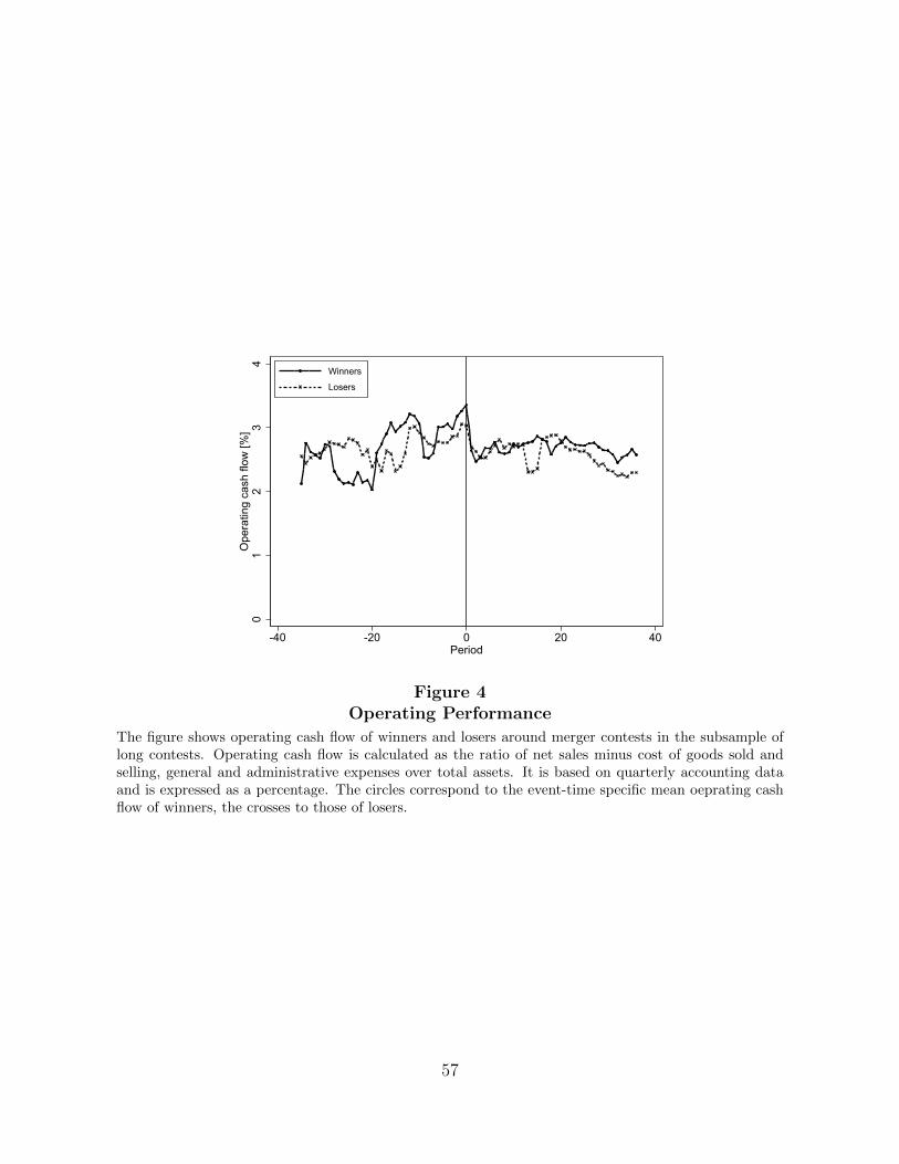
01

23

4O

pera

ting

cash

flow

[%]

-40 -20 0 20 40Period

Winners

Losers

Figure 4Operating Performance

The figure shows operating cash flow of winners and losers around merger contests in the subsample oflong contests. Operating cash flow is calculated as the ratio of net sales minus cost of goods sold andselling, general and administrative expenses over total assets. It is based on quarterly accounting dataand is expressed as a percentage. The circles correspond to the event-time specific mean oeprating cashflow of winners, the crosses to those of losers.

57

0.1

.2.3

.4Fr

actio

n of

con

test

s

-400 -300 -200 -100 0 100 200 300 400Winner-loser difference in long-run BHAR

Figure 5Distribution of Merger Effect Estimates

The histogram shows the distribution of the estimated merger effect for all 56 contests of above-medianduration in our Full Sample. The merger effect is the winner-loser difference in the market-adjustedBHAR three years after the merger.

58

.12

.14

.16

.18

.2N

et m

arke

t lev

erag

e

-40 -20 0 20 40Period

WinnersLosers

Figure 6Net Market Leverage

The figure shows net market leverage of winners and losers around merger contests in long contests. Netmarket leverage is defined as debt in current liabilities plus long term debt minus cash and short-terminvestments, divided by total assets minus book equity plus market equity. The variable is computedusing quarterly data. The circles correspond to the event-time specific mean leverage of winners, thecrosses to those of losers.

59

Table 1Descriptive Statistics

Panel A: Bidder Characteristics

Winners Losers p-value of

Mean Median Std N Mean Median Std N mean diff.

Total assets [$m] 12649.91 3107.34 26912.24 111 7202.58 2495.59 10750.64 120 0.04Market value [$m] 19320.16 5351.05 39464.55 111 11628.67 3258.72 21887.65 120 0.07Sales [$m] 6936.18 1709.6 16697.29 111 4063.24 1112.70 8460.92 119 0.10Tobin’s Q 1.88 1.41 1.37 111 1.82 1.36 1.29 120 0.74PP&E 0.29 0.22 0.25 108 0.30 0.22 0.26 116 0.86Profitability 0.12 0.11 0.08 108 0.12 0.12 0.08 116 0.63Book leverage 0.26 0.19 0.21 111 0.23 0.19 0.17 116 0.20Market leverage 0.18 0.15 0.16 111 0.17 0.14 0.14 116 0.52Ann. CAR [%] -1.51 -0.61 7.41 111 -0.44 -0.93 6.66 119 0.25Ann. CAR [$m] -336.28 -6.76 1967.72 111 12.48 -4.97 881.73 118 0.08

Panel B: Deal Characteristics

P25 Median P75 Mean Std N

Deal value [$m] 90.41 501.95 1,186 3016.52 10805.97 109Tender offer 0.00 0.00 1.00 0.37 0.48 111Hostile 0.00 0.00 0.00 0.09 0.29 111Percentage paid in stock 0.00 0.00 68.74 31.19 40.74 111Percentage paid in cash 0.00 35.00 100.00 46.71 44.96 111Number of bidders 2.00 2.00 3.00 2.41 0.91 111Offer premium [% of target] 30.71 51.56 79.28 63.24 63.24 79Offer premium [% of acquiror] 1.59 6.43 18.66 10.08 20.55 79Contest duration [months] 4.00 7.00 10.00 8.65 6.66 111

In Panel A, Total assets are the book value of total assets. Market value is Total assets plus market value ofequity (common shares outstanding times fiscal-year closing price) minus book value of equity (book value ofshareholders’ equity, plus balance sheet deferred taxes and investment tax credit [if available], minus book valueof preferred stock, where, depending on availability, we use redemption, liquidation, or par value (in that order)to estimate the book value of preferred stock). Tobin’s Q is the ratio of Market value to book value of assets.PP&E is book value of property, plant and equipment divided by total assets. Profitability is operating incomebefore depreciation divided by total assets. Leverage is debt in current liabilities plus long term debt, either dividedby Total assets (Book leverage) or by Market value (Market leverage). All of the above variables are based onbalance sheet and income data from the end of the fiscal year preceding the contest. Announcement CAR [%] isthe three-day cumulative market-adjusted return around the announcement date of the winner’s or loser’s first bidin a given contest. Announcement CARs [$m] are three-day cumulative dollar abnormal returns of the first bid,i.e., percentage announcement CARs multiplied by the bidder’s pre-merger market value of equity. p-value of meandifference refers to the difference in means between winners and losers. In Panel B, Deal value is the dollar valueof the winning bid. Tender offer is a dummy indicating a tender offer. Hostile is a dummy indicating whether thedeal attitude of the winning bid was hostile. Percentage paid in stock is the percentage of the winning bid thatis paid in stock. Percentage paid in cash is the percentage paid in cash. Number of bidders is the total numberof bidders involved in the merger contest. Offer premium [% of target] is the run-up in the target’s stock pricefrom 40 days prior to the announcement of the initial bid until completion of the merger contest. Offer premium[% of acquiror] is Offer premium [% of target] times target equity value divided by acquiror equity value. Contestduration is the number of months from the month-end preceding the first bid until the end of the month of thecompletion of the merger.

60

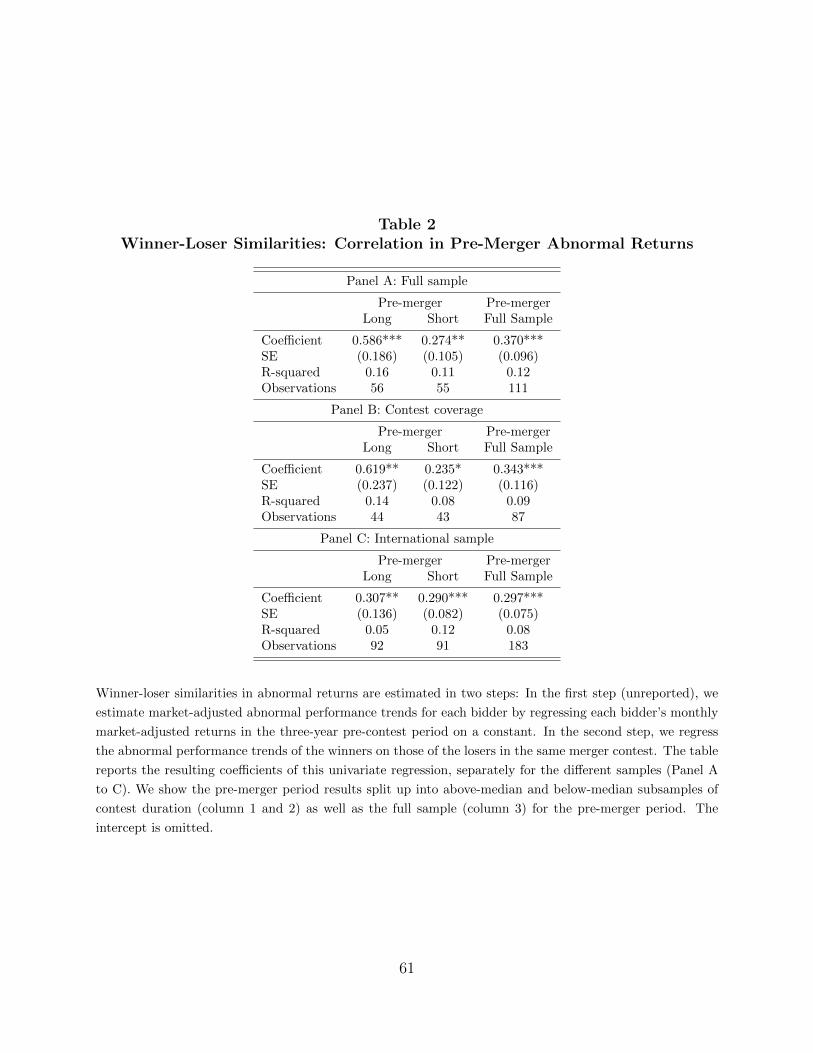
Table 2Winner-Loser Similarities: Correlation in Pre-Merger Abnormal Returns

Panel A: Full sample

Pre-merger Pre-mergerLong Short Full Sample

Coefficient 0.586*** 0.274** 0.370***SE (0.186) (0.105) (0.096)R-squared 0.16 0.11 0.12Observations 56 55 111

Panel B: Contest coverage


Coefficient 0.619** 0.235* 0.343***SE (0.237) (0.122) (0.116)R-squared 0.14 0.08 0.09Observations 44 43 87

Panel C: International sample


Coefficient 0.307** 0.290*** 0.297***SE (0.136) (0.082) (0.075)R-squared 0.05 0.12 0.08Observations 92 91 183

Winner-loser similarities in abnormal returns are estimated in two steps: In the first step (unreported), we

estimate market-adjusted abnormal performance trends for each bidder by regressing each bidder’s monthly

market-adjusted returns in the three-year pre-contest period on a constant. In the second step, we regress

the abnormal performance trends of the winners on those of the losers in the same merger contest. The table

reports the resulting coefficients of this univariate regression, separately for the different samples (Panel A

to C). We show the pre-merger period results split up into above-median and below-median subsamples of

contest duration (column 1 and 2) as well as the full sample (column 3) for the pre-merger period. The

intercept is omitted.

61

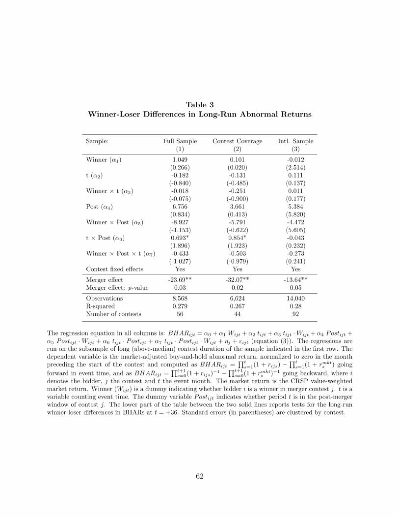
Table 3Winner-Loser Differences in Long-Run Abnormal Returns

Sample: Full Sample Contest Coverage Intl. Sample(1) (2) (3)

Winner (α1) 1.049 0.101 -0.012(0.266) (0.020) (2.514)

t (α2) -0.182 -0.131 0.111(-0.840) (-0.485) (0.137)

Winner × t (α3) -0.018 -0.251 0.011(-0.075) (-0.900) (0.177)

Post (α4) 6.756 3.661 5.384(0.834) (0.413) (5.820)

Winner × Post (α5) -8.927 -5.791 -4.472(-1.153) (-0.622) (5.605)

t × Post (α6) 0.693* 0.854* -0.043(1.896) (1.923) (0.232)

Winner × Post × t (α7) -0.433 -0.503 -0.273(-1.027) (-0.979) (0.241)

Contest fixed effects Yes Yes Yes

Merger effect -23.69** -32.07** -13.64**Merger effect: p-value 0.03 0.02 0.05

Observations 8,568 6,624 14,040R-squared 0.279 0.267 0.28Number of contests 56 44 92

The regression equation in all columns is: BHARijt = α0 + α1 Wijt + α2 tijt + α3 tijt ·Wijt + α4 Postijt +α5 Postijt ·Wijt + α6 tijt · Postijt + α7 tijt · Postijt ·Wijt + ηj + εijt (equation (3)). The regressions arerun on the subsample of long (above-median) contest duration of the sample indicated in the first row. Thedependent variable is the market-adjusted buy-and-hold abnormal return, normalized to zero in the monthpreceding the start of the contest and computed as BHARijt =

∏ts=1(1 + rijs) −

∏ts=1(1 + rmkt

s ) going

forward in event time, and as BHARijt =∏t+1

s=0(1 + rijs)−1 −

∏t+1s=0(1 + rmkt

s )−1 going backward, where idenotes the bidder, j the contest and t the event month. The market return is the CRSP value-weightedmarket return. Winner (Wijt) is a dummy indicating whether bidder i is a winner in merger contest j. t is avariable counting event time. The dummy variable Postijt indicates whether period t is in the post-mergerwindow of contest j. The lower part of the table between the two solid lines reports tests for the long-runwinner-loser differences in BHARs at t = +36. Standard errors (in parentheses) are clustered by contest.

62

Table

4W

inner-

Lose

rD

iffere

nce

sin

Long-R

un

Abnorm

al

Retu

rns

-A

ltern

ati

ve

Retu

rnA

dju

stm

ents

Dep

t.va

riab

le:

BH

AR

(in

d.-

ad

just

ed)

BH

AR

(ris

k-a

dju

sted

)B

HR

(un

ad

just

ed)

Sam

ple

:F

ull

Sam

ple

Conte

stC

over

age

Fu

llS

am

ple

Conte

stC

over

age

Fu

llS

am

ple

Conte

stC

over

age

(1)

(2)

(3)

(4)

(5)

(6)

Win

ner

(α1)

1.48

00.5

52

1.3

51

0.7

75

0.8

11

-0.2

67

(4.1

99)

(5.2

39)

(4.0

08)

(4.9

57)

(3.8

45)

(4.7

72)

t(α

2)

-0.0

59-0

.099

-0.0

20

-0.0

02

0.5

17**

0.5

56*

(0.2

51)

(0.3

03)

(0.1

90)

(0.2

15)

(0.2

47)

(0.3

13)

Win

ner

×t

(α3)

0.12

5-0

.072

-0.1

01

-0.3

04

-0.0

45

-0.2

70

(0.3

35)

(0.4

11)

(0.2

41)

(0.2

72)

(0.2

41)

(0.2

77)

Pos

t(α

4)

6.69

62.8

60

3.3

02

-0.8

53

22.6

12***

21.4

92**

(7.6

12)

(8.1

10)

(8.7

55)

(9.0

07)

(8.1

53)

(8.8

29)

Win

ner

×P

ost

(α5)

-9.5

35-6

.060

-9.6

25

-7.0

03

-7.9

57

-5.5

02

(7.6

30)

(9.1

54)

(7.8

96)

(9.4

32)

(7.5

95)

(9.2

36)

t×

Pos

t(α

6)

0.64

1*0.9

05**

0.5

24

0.7

44*

0.8

44*

0.9

87*

(0.3

67)

(0.4

47)

(0.3

40)

(0.3

82)

(0.4

66)

(0.5

78)

Win

ner

×P

ost×

t(α

7)

-0.8

64*

-1.0

90*

-0.4

08

-0.5

25

-0.4

21

-0.4

52

(0.4

81)

(0.5

89)

(0.4

40)

(0.5

28)

(0.4

27)

(0.5

17)

Con

test

fixed

effec

tsY

esY

esY

esY

esY

esY

es

Mer

ger

effec

tatt

=36

-33.

90**

*-4

6.1

8***

-26.1

0**

-35.2

3**

-23.4

5**

-31.0

3**

Mer

ger

effec

t:p

-val

ue

0.00

0.0

00.0

50.0

30.0

40.0

2

Ob

serv

atio

ns

8,41

96,5

09

8,5

68

6,6

24

8,5

68

6,6

24

R-s

qu

ared

0.27

0.2

30.2

60.2

60.3

60.3

6N

um

ber

ofco

nte

sts

5644

56

44

56

44

Th

ere

gres

sion

equat

ion

inal

lco

lum

ns

is:BHAR

ijt

=α0

+α1W

ijt

+α2t ijt

+α3t ijt·W

ijt

+α4Post ijt

+α5Post ijt·W

ijt

+α6t ijt·

Post ijt

+α7t ijt·Post ijt·W

ijt

+η j

+ε i

jt

(equ

ati

on

(3))

.T

he

regre

ssio

ns

are

run

on

the

sub

sam

ple

of

lon

g(a

bov

e-m

edia

n)

conte

std

ura

tion

ofth

esa

mp

lein

dic

ated

inth

efi

rst

row

.T

he

dep

end

ent

vari

ab

leis

the

bu

y-a

nd

-hold

cum

ula

tive

ab

norm

al

retu

rn,

norm

alize

dto

zero

inth

em

onth

pre

ced

ing

the

star

tof

the

conte

stan

dco

mp

ute

dasBHAR

ijt

=∏ t s

=1(1

+r i

js)−

∏ t s=1(1

+rb

mijs)

goin

gfo

rward

inev

ent

tim

e,an

d

asBHAR

ijt

=∏ t+1 s

=0(1

+r i

js)−

1−

∏ t+1 s=0(1

+rb

mijs)−

1goin

gb

ack

ward

,w

her

ei

den

ote

sth

eb

idd

er,j

the

conte

st,t

the

even

tm

onth

,an

dbm

refe

ren

ces

ab

ench

mar

kp

ortf

olio

.In

colu

mn

1an

d2,

the

ben

chm

ark

retu

rnis

the

valu

e-w

eighte

din

du

stry

retu

rnu

sin

gth

eF

am

a-F

ren

ch12

-in

du

stry

clas

sifi

cati

on.

Th

eb

ench

mar

kre

turn

inco

lum

ns

3an

d4

isth

eC

AP

Mre

qu

ired

retu

rn,r f

t+βi(r m

t−r f

t).

Colu

mn

s5

an

d6

use

the

raw

,un

adju

sted

bu

y-a

nd

-hol

dre

turn

,i.

e.th

eb

ench

mark

retu

rnis

set

toze

ro.

Win

ner

(Wijt)

isa

du

mm

yin

dic

ati

ng

wh

eth

erb

idd

eri

isa

win

ner

inm

erge

rco

nte

stj.t

isa

vari

able

cou

nti

ng

even

tti

me.

Th

ed

um

my

vari

ab

lePost ijt

ind

icate

sw

het

her

per

iodt

isin

the

post

-mer

ger

win

dow

ofco

nte

stj.

Th

elo

wer

par

tof

ofth

eta

ble

bet

wee

nth

etw

oso

lid

lin

esre

port

ste

sts

for

the

lon

g-r

un

win

ner

-lose

rd

iffer

ence

sin

BH

AR

satt

=+

36.

Sta

nd

ard

erro

rs(i

np

aren

thes

es)

are

clu

ster

edby

conte

st.

63

Table 5Winner-Loser Differences in Long-Run Abnormal Returns - Robustness

Interaction variable: Acq. Q Publ./priv. No. bidders Acq. premium(1) (2) (3) (4)

Winner (α1) -3.591 5.622 -0.440 -0.644(6.811) (4.733) (5.687) (9.380)

t (α2) -0.224 0.252 -0.374 -0.247(0.258) (0.231) (0.335) (0.381)

Winner × t (α3) -0.472 0.087 0.207 -0.472(0.365) (0.309) (0.333) (0.492)

Post merger (α4) 11.366 2.624 3.155 -3.295(9.935) (12.746) (10.992) (15.230)

Winner × Post (α5) -9.173 -17.261* -12.433 1.077(8.351) (9.675) (10.605) (16.292)

t × Post (α6) 0.956** 0.613 0.842 0.115(0.382) (0.682) (0.535) (0.580)

Winner × Post × t (α7) 0.089 0.685 -0.559 -0.251(0.464) (0.794) (0.557) (0.734)

Interaction × Winner (α9) 8.476 -5.829 3.351 0.204(7.670) (6.822) (6.792) (9.821)

Interaction × t (α10) 0.091 -0.569 0.483 -0.136(0.446) (0.360) (0.387) (0.552)

Interaction × Winner × t (α11) 0.900* -0.117 -0.588 0.877(0.497) (0.432) (0.424) (0.575)

Interaction × Post (α12) -10.015 5.423 9.075 21.776(16.401) (16.150) (15.986) (19.570)

Interaction × Post × Winner (α13) 1.287 10.443 13.036 -14.883(15.736) (13.657) (14.987) (19.395)

Interaction × Post × t (α14) -0.572 0.105 -0.375 1.158(0.764) (0.807) (0.682) (0.849)

Interaction × Post × t × Winner (α15) -1.000 -1.426 0.304 -0.932(0.864) (0.933) (0.814) (0.969)

Merger effect for interaction=0 (p-value) -26.15** (0.01) 15.39 (0.59) -25.20* (0.06) -24.86 (0.12)Merger effect for interaction=1 (p-value) -19.90 (0.31) -34.02*** (0.01) -18.76 (0.29) -41.46*** (0.01)Difference in merger effect (p-value) 6.25 (0.77) -49.41 (0.11) 6.43 (0.77) -16.60 (0.46)

Observations 8,568 8,568 8,568 6,624R-squared 0.28 0.29 0.29 0.29Number of contests 56 56 0.56 44

The regression equation is BHARijt = α0 + α1Wijt + α2 tijt + α3 tijtWijt + α4 Postijt + α5 PostijtWijt +α6 tijt Postijt+α7 tijt PostijtWijt+Interactionsijt+ηj+εijt, where i denotes the bidder, j the contest and tthe event month. The dependent variable is the market-adjusted buy-and-hold abnormal return, normalizedto zero in the month preceding the start of the contest. The market return is the CRSP value-weightedmarket return. Wijt indicates whether bidder i is a winner in merger contest j; t counts event time; andPostijt indicates whether period t is in the post-merger window of contest j. For columns (1) and (4),Interaction indicates the above-median subsample in terms of acquiror Q and acquisition premium, forcolumn (2), it indicates a public target, and for (3) contests with more than two bidders. Acquiror Q isthe ratio of the acquiror’s market value to book value of assets. The takeover premium is computed asthe runup in the target’s stock price from 40 trading days prior to the beginning of the contest until oneday after completion. The lower part of the table between the two solid lines reports tests for the long-runwinner-loser differences in BHARs at t = +36. Standard errors (in parentheses) are clustered by contest.

64

Table

6W

inner-

Lose

rD

iffere

nce

sin

Long-R

un

Abnorm

al

Retu

rns

-In

tera

ctio

nE

ffect

s

Dep

end

ent

vari

able

:B

HA

R(m

ark

et-a

dju

sted

)In

tera

ctio

nva

riab

le:

All

-cash

Div

ersi

f.A

cqsi

zeT

gt

size

Host

ile

Tgtα

Tgt

pro

fit

Tgt

Q(1

)(2

)(3

)(4

)(5

)(6

)(7

)(8

)

Win

ner

(α1)

0.2

86

1.4

99

-2.6

89

0.3

18

1.2

10

-7.7

19

4.8

31

5.0

52

(4.2

86)

(4.2

96)

(7.2

78)

(7.1

76)

(4.1

35)

(9.7

80)

(3.4

02)

(3.1

44)

t(α

2)

-0.0

54

-0.2

46

-0.4

43

-0.3

29

-0.1

86

-0.5

06

-0.2

95

-0.6

75

(0.1

82)

(0.2

41)

(0.4

08)

(0.4

00)

(0.2

28)

(0.3

94)

(0.4

36)

(0.4

37)

Win

ner

×t

(α3)

-0.0

60

0.0

15

-0.1

09

0.0

34

-0.0

10

-0.6

67

0.1

14

0.2

00

(0.2

40)

(0.2

72)

(0.4

53)

(0.4

18)

(0.2

58)

(0.4

90)

(0.3

83)

(0.3

53)

Pos

tm

erge

r(α

4)

6.7

20

10.7

72

-8.4

60

6.2

69

7.5

15

-5.2

82

-2.8

25

14.9

95

(8.7

88)

(8.6

31)

(11.7

84)

(13.0

66)

(8.2

88)

(15.1

28)

(11.5

47)

(12.1

28)

Win

ner

×P

ost

(α5)

-9.7

63

-10.8

54

1.9

28

-7.8

71

-10.1

17

7.5

01

3.1

86

-21.0

86**

(8.2

77)

(8.6

41)

(11.3

07)

(10.9

69)

(8.1

25)

(14.0

03)

(9.8

52)

(9.7

67)

t×

Pos

t(α

6)

0.5

34

0.6

70*

1.2

37*

0.6

83

0.6

59*

1.5

81***

1.4

39**

1.6

50**

(0.3

45)

(0.3

80)

(0.6

29)

(0.5

59)

(0.3

79)

(0.5

25)

(0.5

64)

(0.6

77)

Win

ner

×P

ost×

t(α

7)

-0.2

54

-0.2

65

-0.6

28

-0.3

11

-0.2

91

-0.8

51

-1.1

93

-1.1

74

(0.4

29)

(0.4

48)

(0.7

01)

(0.5

79)

(0.4

24)

(0.8

22)

(0.7

23)

(0.7

49)

Inte

ract

ion×

Win

ner

(α9)

10.3

50

-3.4

52

7.5

64

0.7

02

-3.7

78

12.4

16

-10.1

02

-11.2

52

(8.7

72)

(9.5

83)

(7.8

44)

(7.9

73)

(10.4

32)

(10.5

64)

(11.2

88)

(10.6

98)

Inte

ract

ion×

t(α

10)

-1.6

13

0.5

75*

0.5

30

0.2

89

0.0

81

0.7

64*

-0.2

35

0.6

64

(1.6

19)

(0.3

18)

(0.4

23)

(0.4

42)

(0.3

06)

(0.4

39)

(0.6

01)

(0.5

96)

Inte

ract

ion×

Win

ner

×t

(α11)

0.6

41

-0.2

92

0.1

74

-0.1

00

-0.1

66

1.0

32*

-0.3

06

-0.5

32

(1.3

97)

(0.3

62)

(0.4

87)

(0.4

96)

(0.4

24)

(0.5

81)

(0.6

36)

(0.6

37)

Inte

ract

ion×

Pos

t(α

12)

0.4

56

-36.1

44*

30.9

23*

1.2

38

-15.9

41

19.7

17

3.6

31

-26.7

07

(13.7

20)

(20.8

83)

(15.7

33)

(16.5

32)

(40.4

54)

(21.5

87)

(19.2

66)

(18.8

56)

Inte

ract

ion×

Pos

t×

Win

ner

(α13)

9.3

16

16.6

47

-22.2

01

-2.1

85

23.9

93*

-21.6

59

-10.9

90

33.4

75

(20.3

22)

(12.4

07)

(15.4

34)

(15.8

54)

(12.2

56)

(20.2

10)

(21.0

04)

(20.0

58)

Inte

ract

ion×

Pos

t×

t(α

14)

2.0

05

0.2

12

-1.1

06

0.0

24

0.7

13

-1.8

97**

-0.9

22

-1.6

45*

(2.1

25)

(1.3

39)

(0.7

26)

(0.7

46)

(1.2

84)

(0.7

15)

(0.8

76)

(0.8

72)

Inte

ract

ion×

Pos

t×

t×

Win

ner

(α15)

-2.2

31

-1.5

62

0.4

08

-0.3

84

-2.7

32

0.3

74

0.8

71

0.9

90

(1.8

43)

(1.2

24)

(0.8

46)

(0.8

51)

(2.1

54)

(0.9

93)

(1.0

65)

(1.0

61)

(Tab

leco

nti

nu

edon

nex

tp

age)

65

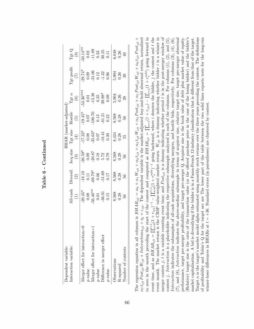
Table

6-

Conti

nued

Dep

end

ent

vari

able

:B

HA

R(m

ark

et-a

dju

sted

)In

tera

ctio

nva

riab

le:

All

-cash

Div

ersi

f.A

cqsi

zeT

gt

size

Host

ile

Tgtα

Tgt

pro

fit

Tgt

Q(1

)(2

)(3

)(4

)(5

)(6

)(7

)(8

)

Mer

ger

effec

tfo

rin

tera

ctio

n=

0-2

0.4

5*

-18.1

0-2

6.5

9*

-17.2

3*

-19.4

5*

-53.3

6***

-29.7

4*

-50.1

4**

p-v

alu

e0.0

80.1

10.0

90.0

80.0

70.0

10.0

90.0

2M

erge

reff

ect

for

inte

ract

ion

=1

-56.4

6**

-69.7

9*

-20.8

7-3

5.6

3*

-100.7

0-1

3.3

8-3

1.0

6-1

1.8

9p

-val

ue

0.0

10.0

60.1

80.0

70.1

30.3

50.1

20.3

3D

iffer

ence

inm

erge

reff

ect

-36.0

1-5

1.6

95.7

2-1

8.4

1-8

1.2

139.9

8*

-1.3

238.2

5p

-val

ue

0.1

50.1

70.7

90.3

90.2

20.0

90.9

60.1

1

Ob

serv

atio

ns

8,5

68

8,5

68

8,5

68

8,4

24

8,5

68

5,9

04

5,9

04

6,0

48

R-s

qu

ared

0.2

80.2

80.2

90.2

80.2

80.2

60.2

60.2

6N

um

ber

ofco

nte

sts

56

56

56

55

56

39

39

40

Th

ere

gres

sion

equ

atio

nin

all

colu

mn

sisBHAR

ijt

=α0

+α1W

ijt

+α2t ijt

+α3t ijtW

ijt

+α4Post ijt

+α5Post ijtW

ijt

+α6t ijtPost ijt

+α7t ijtPost ijtW

ijt

+Interactions i

jt

+η j

+ε i

jt.

Th

edep

end

ent

vari

ab

leis

the

mark

et-a

dju

sted

bu

y-a

nd-h

old

ab

norm

al

retu

rn,

norm

ali

zed

toze

roin

the

mon

thp

rece

din

gth

est

art

ofth

eco

nte

stan

dco

mp

ute

dasBHAR

ijt

=∏ t s

=1(1

+r i

js)−

∏ t s=1(1

+rm

kt

s)

goin

gfo

rward

in

even

tti

me,

and

asBHAR

ijt

=∏ t+1 s

=0(1

+r i

js)−

1−

∏ t+1 s=0(1

+rm

kt

s)−

1goin

gb

ack

ward

,w

her

ei

den

ote

sth

eb

idd

er,j

the

conte

stan

dt

the

even

tm

onth

.T

he

mar

ket

retu

rnis

the

CR

SP

valu

e-w

eighte

dm

ark

etre

turn

.W

ijt

isa

du

mm

yin

dic

ati

ng

wh

eth

erb

idd

eri

isa

win

ner

inm

erge

rco

nte

stj;t

isa

vari

able

cou

nti

ng

even

tti

me;

an

dPost ijt

isa

du

mm

yin

dic

ati

ng

wh

eth

erp

erio

dt

isin

the

post

-mer

ger

win

dow

of

conte

stj.Interaction

isa

pla

ceh

old

erin

dic

atin

gth

ere

spec

tive

sub

sam

ple

an

aly

zed

inea

chof

the

colu

mn

s.F

or

colu

mn

s(1

),(2

),an

d(5

),Interaction

ind

icat

esth

esu

bsa

mp

les

ofal

l-ca

shacq

uis

itio

ns,

div

ersi

fyin

gm

erger

s,an

dh

ost

ile

bid

s,re

spec

tive

ly.

For

colu

mn

s(3

),(4

),(6

),(7

),an

d(8

),Interaction

ind

icat

esth

eab

ove-

med

ian

sub

sam

ple

inte

rms

of

acq

uir

or

size

,re

lati

veta

rget

size

,ta

rget

pre

-mer

ger

ab

norm

al

per

form

ance

,ta

rget

pre

-mer

ger

pro

fita

bil

ity,

and

targ

etp

re-m

erger

Q.

Acq

uir

or

size

isth

eb

ook

valu

eof

deb

tp

lus

mark

etva

lue

of

equit

y.(R

elat

ive)

targ

etsi

zeis

the

rati

oof

the

tran

sact

ion

valu

e(o

rth

eoff

ered

purc

hase

pri

cein

the

case

of

the

losi

ng

bid

der

)an

dth

eb

idd

er’s

mar

ket

cap

ital

izat

ion

.A

bid

isd

iver

sify

ing

ifth

eb

idd

eris

ina

Fam

a-F

ren

ch12-i

nd

ust

rycl

ass

ifica

tion

that

isd

iffer

ent

from

that

of

the

targ

et.

Tar

getα

isth

eta

rget

’sm

arke

tm

od

elal

ph

aes

tim

ate

du

sin

gm

onth

lyst

ock

retu

rns

over

the

thre

eyea

rsp

rece

din

gth

eco

nte

st.

Th

ed

efin

itio

ns

ofp

rofi

tab

ilit

yan

dT

obin

’sQ

for

the

targ

etar

eare

Th

elo

wer

part

of

the

tab

leb

etw

een

the

two

soli

dli

nes

rep

ort

ste

sts

for

the

lon

g-r

un

win

ner

-los

erd

iffer

ence

sin

BH

AR

satt

=+

36.

Sta

nd

ard

erro

rs(i

np

are

nth

eses

)are

clu

ster

edby

conte

st.

66

Table 7Alternative Methods to Assess the Returns to Mergers – Comparison

Panel A: Estimates from traditional methods

Mean SE N

Winners’ announcement CAR [%] -1.097 (0.799) 56

Winners’ CAR at loser’s withdrawal [%] -0.095 (0.824) 55

Losers’ CAR at loser’s withdrawal [%] 1.798** (0.715) 62

Winners’ 4-factor alpha × (36+avg contest duration) 10.335 (10.467) 56

Winners’ market-adjusted BHAR [%] 0.097 (13.315) 56

Panel B: Correlation with estimates from traditional methods

Coefficient SE N

Winners’ announcement CAR [%] -3.496 (2.288) 56

Winners’ CAR at loser’s withdrawal [%] 3.821 (2.262) 56

Losers’ CAR at loser’s withdrawal [%] 0.504 (2.243) 62

Winners’ market-adjusted BHAR [%] 0.649*** (0.108) 56

Panel A reports the three-day market-adjusted return to the aquiror at announcement of the acquiror’sinitial bid (first row) and at the announcement of the loser’s withdrawal (second row), the return to theloser at withdrawal (third row), the four-factor alpha of equally-weighted calendar-month portfolios of post-acquisition acquiror returns (fourth row), and the long-run buy-and-hold market-adjusted return of acquirors(fifth row). The four-factor alpha is the intercept of a time-series regression of the equally weighted excessreturn of an acquiror portfolio on the excess market return, the Fama-French factors, and the momentumfactor. We use all acquiror stock returns that occur during the contest period or the following 36 months.The four-factor alpha from the monthly return regression is multiplied by 36 plus the average contest dura-tion to make it comparable to the performance measurement period used for the estimates in Table 3. PanelB reports univariate regressions of the long-run winner-loser difference in BHARs on the return at announce-ment of the acquiror’s initial bid (first row) and at the announcement of the loser’s withdrawal (second row),the return to the loser at withdrawal (third row), and the long-run buy-and-hold market-adjusted return ofacquirors (last row). Standard errors are in parentheses.

67

Appendix: Sample Construction

In this Appendix, we provide more details on the construction of our data set from Thomson

One Mergers and Acquisitions, CRSP, Compustat, Compustat Global, Datastream, and

I/B/E/S.

The initial data collection from Thomson One for the two North American samples

described in the main paper includes the following variables: deal number of each bid,

acquiror’s and target’s company identifiers (CIDGEN), six-digit CUSIP, nation, SIC code,

announcement date of the bid, its effective or withdrawal date, dollar value of the offer,

percentage of the transaction value offered in cash, in stock, or in other means of payment,

deal attitude (friendly or hostile), number of bidders involved in the bidding process, and

competing bid flag. We collect those data items for the period from 1/1/1985 to 12/31/2012.

We collect the following data for the longer period (including +/- three years) of 1/1/1982

to 12/31/2015: From the CRSP Monthly Stock Database, we obtain holding period stock

return (RET), distribution event code (DISTCD), delisting code (DLSTCD), date of delisting

payment (DLPDT), amount after delisting (DLAMT), delisting return (DLRET), and CRSP

value-weighted index returns (VWRETD). From the Fama-French data library, we obtain

the monthly Fama-French factor returns (MKTRF, SMB, HML), the risk-free rate, and

value-weighted industry returns (12-industry classification). From the CRSP-COMPUSTAT

Fundamentals Annual Database we obtain yearly accounting data, including total assets

(AT), net sales (SALE), total debt (LT), shareholders’ equity (SEQ), deferred taxes and

investment tax credit (TXDITC), preferres stock liquidating, redemption and carrying value

(PSTKL, PSTKRV, UPSTK, respectively), common shares outstanding (CSHO), fiscal year

closing price (PRCC F), and operating income (OIBDP). From the CRSP-COMPUSTAT

Fundamentals Quarterly Database, we obtain quarterly data on total assets (ATQ), debt

in current liabilities (DLCQ), long-term debt (DLTTQ), cash and short-term investments

68

(CHEQ), common shares outstanding (CSHOQ), fiscal quarter closing price (PRCCQ), book

value of shareholders’ equity (SEQQ), balance sheet deferred taxes and investment tax credit

(TXDITCQ), book value of preferred stock (PSTKQ), net sales (SALEQ), cost of goods sold

(COGSQ), and selling, general and administrative expenses (XSGAQ). We use the CRSP-

COMPUSTAT quarterly data to construct the time series of operating cash flow and various

measures of leverage (book and market leverage, as well as net book and net market leverage)

for each bidder.

We merge the Thomson One and CRSP data using the 6-digit CUSIPs. Specifically,

we match the 6-digit CUSIP provided by Thomson One with the first six digits of CRSP’s

historical CUSIP (NCUSIP). Since the CUSIP of a firm can change over time, and reassign-

ment of CUSIPs is particularly common following a merger, we match Thomson One’s bidder

CUSIP with CRSP’s NCUSIP for the month preceding the announcement of the bid. We

manually check that the company names recorded by Thomson correspond to the matched

CRSP company names. If a firm has multiple equity securities outstanding, we use (1) the

common stock if common and other types of stock are traded; (2) Class A shares if the

company has Class A and Class B outstanding; and (3) the stock with the longest available

time series of data if there are multiple types of common stock traded.

We use the stock return data to construct the monthly time series of bidder returns for

a window of +/− three years around the merger contest (from event time t = −35 to event

time t = +36). Depending on the duration of the bidding contest, the length of the return

time series vary. The CRSP holding period return is adjusted for stock splits, exchanges,

and cash distributions. (This adjustment is important since these events are particularly

common around mergers.) We then construct the corresponding time series of CRSP value-

weighted market returns and of value-weighted industry returns. From these return series

we construct buy-and-hold abnormal returns as described in Section 2.

For publicly listed target firms, we also construct time series of daily returns to calculate

69

the offer premium, computed as the percentage run-up in stock price from 40 trading days

prior to the beginning of the contest until the day of delisting. Alternatively, we express

the offer premium as a percentage of the acquirors’ equity value (percentage run-up in the

target stock price × target market capitalization / acquiror market capitalization).

In the three-year period after a merger, many bidders disappear from CRSP due to delist-

ing. To reduce survivorship bias, we calculate the return implications of the delisting events

for shareholders using all delisting information available in CRSP. The delisting code (DL-

STCD) classifies delistings into mergers, exchanges for other stock, liquidations, and several

other categories of dropped firms; the distribution information (DIVAMT) reports to what

extent shareholders were paid in cash or stock; and the delisting return (DLRET) provides

the shareholder returns from the last day the stock was traded to the earliest post-delisting

date for which CRSP could ascertain the stock’s value. We round the delisting return period

to full months and track the performance of a delisted firm from the perspective of a buy-

and-hold investor, mirroring our approach when tracking the performance of bidders who are

listed. Specifically, we assume that stock payments in takeovers are held in the stock of the

acquiring firm and exchanges for other stock are held in the new stock. When shareholders

receive cash payments (in mergers, liquidations, and bankruptcies) or CRSP cannot identify

or does not cover the security in which payments are made, we track performance as if all

proceeds were invested in the market portfolio, using the value-weighted CRSP index.

We merge the resulting monthly panel with the annual and the quarterly accounting data

from CRSP-COMPUSTAT by assigning, to each monthly observation, the data pertaining

to the most recent preceding fiscal-year (fiscal-quarter) end.

Our initial sample contains 623 bids and 293 takeover contests. We drop repeated bids

by the same bidder, and keep the date of the first bid as the announcement date. This

eliminates 20 bids. Next, we drop 57 contests that had not been completed by March 31,

2012. We further drop 99 bidders that could not be matched to a CRSP PERMNO. We then

70

delete 14 contests in which the winner is the ultimate parent company of the target. Next,

we balance the sample by requiring non-missing stock return data from t = −35 to t = +36

(i.e., from three years before to three years after the contest), which reduces the number

of contests to 178. We also eliminate one bidder which exhibits extreme stock returns and

return volatility in the pre-merger period due to idiosyncratic factors.34 Finally, we keep only

those contests for which we have stock price data for both the winner and the loser(s) in a

given contest. This reduces the sample by another 66 contests, resulting in a final sample of

112 contests with bids placed by 233 bidders, 112 winners and 121 losers (Full Sample).

[Figure A-1 approximately here]

[Table A-1 approximately here]

We add analyst forecast data from I/B/E/S. Specifically, we download the 2-year-ahead

consensus forecast (i.e. the median (MEDEST) and mean (MEANEST) forecast of all an-

alysts covering the firm) of earnings per share for the entire -3/+3-year window around

the merger from the I/B/E/S summary history file using the 8-digit CUSIP as identifier.

As in previous literature, we drop observations with negative forecasted earnings (see, e.g.,

Richardson, Sloan, and You (2011)). We also download forecasts of various other horizons

which yield very similar results.

We extract two-years-ahead earnings forecasts for the 36 months before (and, for com-

pleteness, for the 36 months after) the merger from the I/B/E/S summary history file. We

construct the forecasted-earnings-to-price ratios (FE/P ratios) as the two-year consensus

34 This is the contest between Yahoo! Inc and TMP Worldwide Inc for HotJobs.com Ltd initiated byTMP Worldwide Inc on 29 June 2001 and won by Yahoo! Inc on February 13, 2002. Yahoo! Inc showsa 1000% stock price runup and reversal in the 36 months leading up to the merger, TMP Worldwide Incshows a 100% runup and reversal in the same period. Idiosyncratic factors determining the run-ups makethese bidders a poor benchmark for each other. Keeping the observation in the sample does not affect themagnitude of our findings; it only increases the standard errors.

71

(mean) forecast divided by the stock price at the end of the month.35 Our sample includes

forecasts for 180 firms, 77.2% of our total sample.36

For the International Sample, we obtain the stock returns of non-North American firms in

a three-step procedure. In the first step, we are able to match 59 non-North American firms

with Compustat Global via the SEDOL identifier provided by Thomson One. The firms that

cannot be matched with Compustat Global are then merged with Datastream, also using

the SEDOL. We are able to match 13 firms in this second step. For the remaining firms,

we search annual reports and company profiles for their company identifiers. If no SEDOL

but the International Securities Identification Number (ISIN) can be found, the ISIN is used

as identifier. Finally, we merge these firms with Datastream again, successfully matching

another 18 firms. Daily Compustat Global and Datastream stock prices are compounded to

monthly returns and adjusted for stock splits and dividends. Eventually, we are able to add

152 bids and 72 contests to our North American sample.37

[Table A-2 approximately here]

35 As in previous literature, we drop observations with negative forecasted earnings (see, e.g., Richardson,Sloan, and You (2011)). Alternatively, we use the median forecast and different forecast horizons with verysimilar results.

36 Since firms are covered by analysts at different points in time and for different periods of time, thenumber of available consensus forecasts varies across periods. The average number of available consensusforecasts is 171, which constitutes 73.4% of our total sample.

37 We drop the contest between Volkswagen and General Motors for Skoda. According to Thomson One,the contest starts on 12th September 1990 and ended on the 12th December 1995. However, the corporatehistory states that a decision for Volkswagen was been made as early as December 1990. The discrepancybetween Thomson One and the corporate history is possibly due to the structure of the merger. Skodaremained a joint venture between Volkswagen and the Czech Republic, and Volkswagen only increased itsownership share of the joint venture (above 50%) on Dec 11, 1995. Hence, uncertainty about the outcomeof the contest was resolved significantly before the official completion date.

72

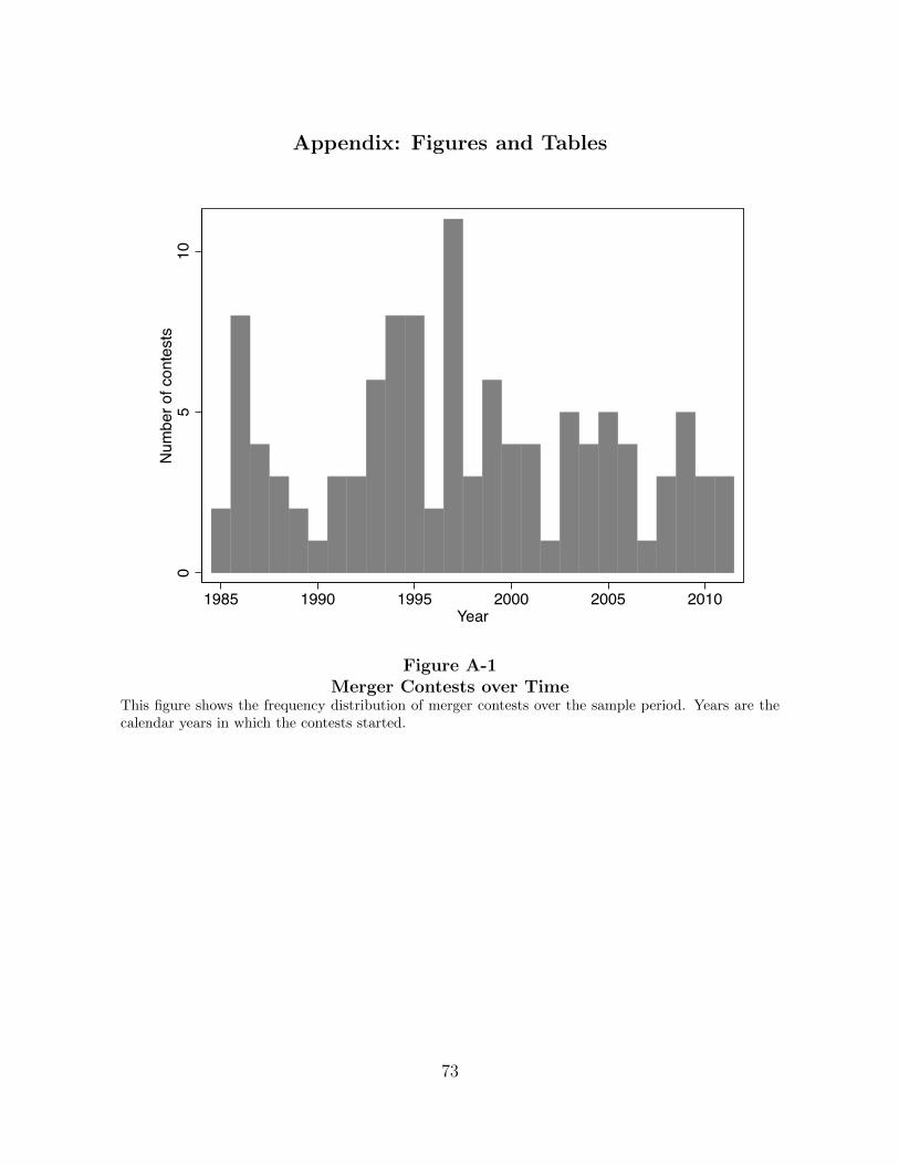
Appendix: Figures and Tables

05

10N

umbe

r of c

onte

sts

1985 1990 1995 2000 2005 2010Year

Figure A-1Merger Contests over Time

This figure shows the frequency distribution of merger contests over the sample period. Years are thecalendar years in which the contests started.

73

-50

-25

025

50

-40 -20 0 20 40Period

Winners

Losers

(a) Contest duration: Upper half

-50

-25

025

50

-40 -20 0 20 40Period

WinnersLosers

(b) Contest duration: Lower half

Figure A-2Winner and Loser Abnormal Performance - Long and Short Contests

The two graphs show the stock price performance of winners and losers around merger contests of long(left panel) and short (right panel) duration. The performance measure is the market-adjusted buy-and-hold return (BHAR), calculated as described in Table 3. The circles correspond to the average winnerBHARs, the crosses to the average loser BHARs.

74

Table

A-1

Sam

ple

Const

ruct

ion

Sam

ple

sele

ctio

ncr

iter

ion

Bid

sB

idd

ers

Win

ner

sL

ose

rsC

onte

sts

Init

ial

sam

ple

623

604

239

365

293

less

rep

eate

db

ids

ofsa

me

bid

der

for

sam

eta

rget

603

603

238

365

292

less

conte

sts

that

wer

en

otco

mp

lete

d488

488

238

250

235

less

bid

der

sw

ith

out

CR

SP

PE

RM

NO

389

389

191

198

208

less

conte

sts

wh

ere

win

ner

was

par

ent

com

pany

362

362

176

186

194

less

bid

der

sw

ith

mis

sin

gre

turn

dat

ain

the

+/-

thre

e-ye

ar

even

tw

ind

ow304

304

154

150

178

less

bid

der

sw

ith

extr

eme

retu

rnvo

lati

lity

303

303

153

150

178

less

bid

der

sin

conte

sts

wit

hm

issi

ng

win

ner

or

lose

r233

233

112

121

112

less

conte

sts

wit

hfi

nan

cial

bid

der

231

231

111

120

111

Th

ein

itia

lsa

mp

leco

nsi

sts

ofal

lb

ids

inco

nte

sted

mer

ger

ssu

bm

itte

dby

pu

bli

cU

.S-l

iste

dco

mp

an

ies

bet

wee

nJanu

ary

1,

1985

an

dM

arc

h31,

2012

and

reco

rded

inth

eT

hom

son

On

eM

erge

rsan

dA

cqu

isit

ion

sd

ata

base

,ex

clu

din

gb

ids

by

Wh

ite

Kn

ights

.W

eap

ply

the

crit

eria

bel

owto

obta

ina

bal

ance

dan

dm

atch

edsa

mp

le,

that

is,

asa

mp

lew

ith

com

ple

ted

ata

on

stock

retu

rns

for

both

the

win

ner

an

dth

elo

ser(

s)in

the

thre

e-ye

arp

erio

ds

bef

ore

and

afte

rth

em

erge

rco

nte

st.

75

Table

A-2

Sam

ple

Const

ruct

ion

-In

tern

ati

onal

Sam

ple

Sam

ple

sele

ctio

ncr

iter

ion

Bid

sB

idd

ers

Win

ner

sL

ose

rsC

onte

sts

Init

ial

sam

ple

1154

997

421

689

539

less

rep

eate

db

ids

ofsa

me

bid

der

for

sam

eta

rget

1129

994

418

689

536

less

conte

sts

that

wer

en

otco

mp

lete

d898

815

418

459

427

less

bid

der

sfo

rw

hic

hn

ost

ock

dat

aco

uld

be

fou

nd

847

772

392

435

404

less

conte

sts

wh

ere

win

ner

was

par

ent

com

pany

615

551

283

316

343

less

bid

der

sw

ith

mis

sin

gre

turn

dat

ain

the

+/-

thre

e-ye

ar

even

tw

ind

ow526

470

244

269

318

less

bid

der

sw

ith

extr

eme

retu

rnvo

lati

lity

523

468

243

268

317

less

bid

der

sin

conte

sts

wit

hm

issi

ng

win

ner

or

lose

r385

357

180

201

184

Nat

ion

ofbid

der

,fi

nal

sam

ple

Un

ited

Sta

tes

247

225

112

113

Can

ada

40

39

15

24

Un

ited

Kin

gdom

37

34

17

17

Au

stra

lia

23

19

811

Fra

nce

10

10

37

Ger

man

y9

94

5Jap

an5

53

2It

aly

54

31

Sp

ain

33

12

Net

her

lan

ds

11

10

Sw

eden

11

10

Sw

itze

rlan

d1

10

1

Th

ein

itia

lsa

mp

leco

nsi

sts

ofal

lb

ids

inco

nte

sted

mer

ger

ssu

bm

itte

dby

pu

bli

cly

list

edco

mp

an

ies

inth

eU

nit

edS

tate

s,C

an

ad

a,

the

Un

ited

Kin

gdom

,A

ust

rali

a,F

ran

ce,

Ger

man

y,Jap

an

,It

aly

,S

pain

,N

eth

erla

nd

s,S

wed

en,

an

dS

wit

zerl

an

db

etw

een

Janu

ary

1,

1985

an

dM

arc

h31,

2012

and

reco

rded

inth

eT

hom

son

On

eM

erge

rsan

dA

cqu

isit

ion

sd

ata

base

,ex

clu

din

gb

ids

by

Wh

ite

Kn

ights

.W

eap

ply

the

crit

eria

bel

owto

obta

ina

bal

ance

dan

dm

atch

edsa

mp

le,

that

is,

asa

mp

lew

ith

com

ple

ted

ata

on

stock

retu

rns

for

both

the

win

ner

an

dth

elo

ser(

s)in

the

thre

e-ye

arp

erio

ds

bef

ore

and

afte

rth

em

erge

rco

nte

st.

76

Table A-3Winner-Loser Differences in Long-Run Abnormal Returns, Short Contests

Sample: Full Sample Contest Coverage Intl. Sample(1) (2) (3)

Winner (α1) 1.110 2.767 2.549(2.423) (2.753) (1.990)

t (α2) -0.117 -0.151 -0.177(0.177) (0.211) (0.155)

Winner × t (α3) 0.137 0.155 0.363**(0.216) (0.265) (0.164)

Post (α4) -0.513 1.262 2.750(4.798) (5.922) (3.950)

Winner × Post (α5) -3.095 -7.319 -1.180(5.842) (7.016) (3.889)

t × Post (α6) -0.457 -0.491 0.292(0.377) (0.428) (0.270)

Winner × Post × t (α7) 0.415 0.577 -0.571*(0.501) (0.618) (0.293)

Contest fixed effects Yes Yes Yes

Merger effect at t = 36 17.32 21.07 -5.89Merger effect: p-value 0.27 0.28 0.49

Observations 8,208 6,480 13,680R-squared 0.28 0.27 0.25Number of contests 56 44 92

The regression equation in all columns is: BHARijt = α0 + α1 Wijt + α2 tijt + α3 tijt ·Wijt + α4 Postijt +α5 Postijt ·Wijt +α6 tijt ·Postijt +α7 tijt ·Postijt ·Wijt + ηj + εijt (equation (3)). The regressions are runon the subsample of short (below-median) contest duration of the sample indicated in the first row. Thedependent variable is the market-adjusted buy-and-hold abnormal return, normalized to zero in the monthpreceding the start of the contest and computed as BHARijt =

∏ts=1(1 + rijs) −

∏ts=1(1 + rmkt

s ) going

forward in event time, and as BHARijt =∏t+1

s=0(1 + rijs)−1 −

∏t+1s=0(1 + rmkt

s )−1 going backward, where idenotes the bidder, j the contest and t the event month. The market return is the CRSP value-weightedmarket return. Winner (Wijt) is a dummy indicating whether bidder i is a winner in merger contest j. t is avariable counting event time. The dummy variable Postijt indicates whether period t is in the post-mergerwindow of contest j. The lower part of the table between the two solid lines reports tests for the long-runwinner-loser differences in BHARs at t = +36. Standard errors (in parentheses) are clustered by contest.

77

Winning by Losing: Evidence on the Long-Run E …moretti/mergers.pdfWinning by Losing: Evidence on...

Documents

Transcript of Winning by Losing: Evidence on the Long-Run E …moretti/mergers.pdfWinning by Losing: Evidence on...