DI

SC

US

SI

ON

P

AP

ER

S

ER

IE

S

Forschungsinstitut zur Zukunft der ArbeitInstitute for the Study of Labor

Winning Big but Feeling No Better? The Effect of Lottery Prizes on Physical and Mental Health

IZA DP No. 4730

January 2010

Bénédicte ApoueyAndrew E. Clark

Winning Big but Feeling No Better?

The Effect of Lottery Prizes on Physical and Mental Health

Bénédicte Apouey University of South Florida

Andrew E. Clark

Paris School of Economics and IZA

Discussion Paper No. 4730 January 2010

IZA

P.O. Box 7240 53072 Bonn

Germany

Phone: +49-228-3894-0 Fax: +49-228-3894-180

E-mail: iza@iza.org

Any opinions expressed here are those of the author(s) and not those of IZA. Research published in this series may include views on policy, but the institute itself takes no institutional policy positions. The Institute for the Study of Labor (IZA) in Bonn is a local and virtual international research center and a place of communication between science, politics and business. IZA is an independent nonprofit organization supported by Deutsche Post Foundation. The center is associated with the University of Bonn and offers a stimulating research environment through its international network, workshops and conferences, data service, project support, research visits and doctoral program. IZA engages in (i) original and internationally competitive research in all fields of labor economics, (ii) development of policy concepts, and (iii) dissemination of research results and concepts to the interested public. IZA Discussion Papers often represent preliminary work and are circulated to encourage discussion. Citation of such a paper should account for its provisional character. A revised version may be available directly from the author.

IZA Discussion Paper No. 4730 January 2010

ABSTRACT

Winning Big but Feeling No Better? The Effect of Lottery Prizes on Physical and Mental Health* We use British panel data to determine the exogenous impact of income on a number of individual health outcomes: general health status, mental health, physical health problems, and health behaviors (drinking and smoking). Lottery winnings allow us to make causal statements regarding the effect of income on health, as the amount won by winners is largely exogenous. Positive income shocks have no significant effect on general health, but a large positive effect on mental health. This result seems paradoxical on two levels. First, there is a well-known status gradient in health in cross-section data, and, second, general health should partly reflect mental health, so that we may expect both variables to move in the same direction. We propose a solution to the first apparent paradox by underlining the endogeneity of income. For the second, we show that lottery winnings are also associated with more smoking and social drinking. General health will reflect both mental health and the effect of these behaviors, and so may not improve following a positive income shock. This paper thus presents the first microeconomic analogue of previous work which has highlighted the negative health consequences of good macroeconomic conditions. JEL Classification: D1, I1, I3 Keywords: income, self-assessed health, mental health, smoking, drinking Corresponding author: Bénédicte Apouey Department of Economics University of South Florida 4202 East Fowler Avenue BSN 3403 Tampa, FL 33620-5500 USA E-mail: benedicte@usf.edu

* Data from the British Household Panel Survey (BHPS) were supplied by the ESRC Data Archive. Neither the original collectors of the data nor the Archive bear any responsibility for the analysis or interpretations presented here. We thank Christophe Chamley, Thierry Debrand, Brigitte Dormont, Fabrice Etilé, Pierre-Yves Geoffard, Florence Jusot, Nicolai Kristensen, Zeynep Or, Andrew Oswald, Lionel Page, Ronnie Schoeb, Jim Taylor and seminar participants at AKF Copenhagen, Alicante, the 2009 BHPS Users’ Conference, Brunel, Cattolica, City University, CREM (Rennes 1), the European Conference on Health Economics (Rome), the 2009 joint congress of the EEA-ESEM (Barcelona), Free University of Berlin, GAINS (Le Mans), the 2008 Journées Louis-André Gérard-Varet (Marseille), ISQOLS 9 (Florence), Lancaster, Maastricht, PSE, Queen Mary and Westfield and the University of South Florida for useful comments.

1. Introduction

The relationship between individual income and health is the subject of what

is by now a very substantial literature, with the broad finding that higher socio-

economic status is associated with better health. This kind of relationship has

now been identified in a large number of countries and for a wide variety of health

variables (see Deaton and Paxson (1999), Marmot and Bobak (2000), Van Doorslaer

et al. (1997), and Winkleby et al. (1992)).

While this association does indeed appear to be widespread, there is less common

ground regarding its causal interpretation. That income, or socio-economic status

more broadly, be correlated with health may indeed reflect a causal effect of the

former on the latter. However, it is entirely possible that poor health also influences

income, by reducing the ability to work for example. In addition, there are likely

hidden common factors that affect both variables, such as the individual’s genetic

endowment, birth weight, or the quality of the school that she attended. In this

case, income and health will be correlated, but not in any causal way.

The vast majority of the existing literature is not able to distinguish between

these three alternative readings of the income-health correlation. Testing the causal

impact of income on health requires exogenous movements in income, which can be

identified in an instrumental or experimental setting. This is the approach to which

we appeal here, using lottery winnings as an exogenous source of income variation

in a large-scale panel dataset.

Most existing work on this question has used a general health status variable as

the dependent variable. We are here able to provide much more detail by assessing

the impact of exogenous changes in income on a number of different health measures:

self-assessed overall health, a psychological measure of mental stress (the 12-item

General Health Questionnaire, or GHQ-12), physical health problems, and health-

related behaviors (smoking and drinking).

The effect of income on these different health variables is far from uniform. There

is first no correlation between lottery winnings and general health. However, this

lack of a relationship actually masks statistically significant correlations in different

health domains. Winning big does indeed improve mental health; however we un-

2

cover counteracting health effects with respect to risky behaviors. Those who win

more on the lottery smoke more and engage in more social drinking, both of which

are likely detrimental to general health. The positive effect on mental health and the

negative effect from risky behaviors may well sum to a negligible overall relationship

between income and general health.

The paper is organized as follows. The following section briefly summarizes the

related literature and discusses our approach. Section 3 presents the data from the

British Household Panel Survey, and Section 4 discusses identification of the effect

of income on health. Section 5 contains the main results, and Section 6 presents

robustness checks and some additional findings. Last Section 7 concludes.

2. Empirical findings on the income-health relationship and our approach

2.1. The causal effect of income on health

Some intuition

It is commonplace to hypothesize that higher income causes better health. If

we assume that individuals maximize a utility function defined over health and

other goods subject to budget and time constraints, a positive shock to income

will loosen the budget constraint and will thus yield better health, if health is a

normal good. However, it seems unlikely that health will be independent of the

other elements of the utility function. We can in particular imagine certain “risky

behaviors” or lifestyle choices which are positively correlated with utility (and which

are themselves also normal goods), but which are negatively correlated with health.

In this case, higher income will have an ambiguous effect on health, by increasing

smoking, drinking or other risky activities which are detrimental to general health.

Findings in the previous literature

The positive relationship between income and health for adults is open to a num-

ber of interpretations, as underlined by Smith (1999): the causality may run from

income to health, from health to income, or both may be determined by hidden com-

mon factors. Below, we discuss the small number of papers that have investigated

this relationship by appealing to exogenous changes in income.

Ettner (1996) estimates the effect of income on health using American data. The

3

health variables she uses are self-assessed health (SAH), a scale of depressive symp-

toms, and daily limitations due to both physical and mental difficulties. The effect

of income on physical and mental health is therefore not systematically separately

evaluated. She addresses the problem of reverse causality via instrumentation, us-

ing the state unemployment rate, work experience, parental education, and spousal

characteristics as instruments. A substantial impact of income on all of the health

variables is found. It can however be countered that the instruments used here are

not exogenous. As noted by Meer et al. (2003), the unemployment rate will only be

a valid instrument if regional variations in health only reflect variations in income,

which may well not be the case.

Lindahl (2002) appeals to Swedish longitudinal data, and constructs an overall

health measure comprised of both the physical and mental aspects of health. Lottery

prizes are used to provide exogenous variations in income.1 A positive causal rela-

tionship between income and this general health measure is found. Exceptionally,

this paper does consider some of the different aspects of health separately. Lottery

winnings are associated with better mental health, lower Body Mass Index, and

have no effect on some physical health problems. However, Lindahl is not able to

evaluate the relationship between lottery wins and smoking drinking, which is at

the heart of our paper.

Meer et al. (2003) use self-assessed health as their main dependent variable,

but also carry out robustness checks using a binary variable indicating physical or

nervous disabilities which limit the individual’s ability to work. In instrumental

variable estimation (using data on inheritances), wealth is not found to have a

1Lottery winnings are an arguably under-exploited source of exogenous variation in income.One of the first systematic uses of which we are aware is Brickman et al. (1978), although in asmall-sample, and cross-sectional, context. Their more recent appearance in panel datasets has ledto their use in what still remains a relatively small number of papers. Apart from work on healthand well-being, described in this Section, they have also appeared in empirical Labor Economics.Henley (2004) considers the determinants of labor supply, and Lindh and Ohlsson (1996) andTaylor (2001) the decision to become self-employed, where lottery gains are supposed to relaxliquidity constraints. Both Henley (2004) and Taylor (2001) use the same database as we do, theBritish Household Panel Survey. A separate literature has traced out the reaction of consumptionand savings to exogenous movements in income. An early example is Bodkin (1959), using anunexpected National Service Life Insurance dividend paid out to World War II veterans in 1950;more recent examples include Imbens et al. (2001), who appeal to differences in winnings amongstmajor-prize winners of the Megabucks Lottery in Massachusetts between 1984 and 1988, and Kuhnet al. (2008), who appeal to differences in winnings in the Dutch postcode lottery.

4

significant effect on health.

Frijters et al. (2005) analyze the relationship between self-assessed health and

income. They try to correct for both reverse causality and hidden common factors,

using an exogenous change in income (due to the fall of the Berlin wall) in a fixed-

effects framework. They find that income has a positive, but only very small, effect

on health.

Last, recent work by Gardner and Oswald (2007) has explored the causality

running from exogenous variations in income (from medium-sized lottery wins) to

changes in mental health, as measured by the GHQ. They find that money has a

significant and positive effect on mental health.

Table 1 summarizes the findings presented above.

2.2. Our approach

We appeal to monetary lottery wins to try to establish a causal link between

exogenous movements in income and changes in a number of different health out-

comes.

We do not construct a score summarizing the different aspects of health, as we

wish to see whether these latter react differently to income shocks, and we clearly

distinguish mental from physical health. Our reason for doing so, unlike most of

the existing literature, comes from the results in Ruhm (2000), which called into

question the notion of one holistic concept of health, in particular in relation to the

economic cycle.

Ruhm (2000) considered various measures of both individual-level and aggregate-

level health, and tracked their movements over periods of boom and bust. His

key finding is that different aspects of health move in different directions during

recessions:

. First, short-run recessions seem to be associated with better physical health. The

common belief that physical health declines during temporary economic con-

tractions is wrong, and mortality is largely procyclical in US data. Regressions

at the US-state level highlight that poor economic conditions are associated

with lower death rates in general, and with reduced prevalence of a number

5

of specific causes of death in particular (cardiovascular diseases, pneumonia,

and motor vehicle accidents). This aggregate relationship is supported by ev-

idence relating individual health outcomes to aggregate economic conditions.

Using individual data from the Behavioral Risk Factor Surveillance system,

Ruhm (2000, 2005) relates individual behaviors to the local unemployment

rate (but not to the individual’s labor-market status). He uncovers significant

behavioral effects, in that individuals modify their lifestyles during short-term

recessions: both tobacco consumption and BMI fall (so that individuals are

more likely to have a healthier body weight), while regular physical activity

increases. Physical health is therefore counter-cyclical, and this specifically

seems to apply to the behavioral correlates of health.

. However, this negative relationship is not found for all of the health measures.

There is one cause of death that is higher during recessions: suicide. As Ruhm

(2001) notes, there is “some evidence that mental health is pro-cyclical”.

Some of these results have been confirmed in recent work by Adda et al. (2009),

who use a structural framework to model the dynamics of income and health, which

latter are considered as stochastic processes. They decompose income into transitory

and permanent components. Adda et al. construct aggregate synthetic cohort

data, and look at the effect of fluctuations in aggregate income (over the 1980s

and 1990s), reflecting macro-economic factors, on health. They find that higher

permanent income has no significant effect on self-reported health, blood pressure,

cardiovascular diseases. The effect of permanent income on mental health is either

negative or insignificant. However, permanent income is positively correlated with

the number of cigarettes smoked per day.

The existing macroeconomic evidence therefore suggests an that physical health

(particularly its behavioral elements) and mental health may not be associated with

exogenous income movements in the same way. However, it has not yet been es-

tablished whether the same results hold at the entirely microeconomic level, when

we correlate different individual health measures with movements in exogenous in-

dividual income. This is what we do below, using data on lottery winnings from

6

nine waves of large-scale panel data.

3. Data

Our data come from the British Household Panel Survey (BHPS), the first wave

of which appeared in 1991. This general survey initially covered a random sample

of around 10,000 individuals in around 5,000 different households in Great Britain;

increased geographical coverage has pushed these figures to around 16,000 and 9,000

respectively in more recent waves. We here make use of lottery data from waves 7 to

15 (1997-2005), as harmonized lottery information is not available in earlier waves.2

The BHPS includes a wide range of information about individual and household

demographics, mental and physical health, labor-force status, employment and val-

ues. There is both entry into and exit from the panel, leading to unbalanced data.

The BHPS is a household panel: all adults in the same household are interviewed

separately. Further details of this survey are available at the following address:

http://www.iser.essex.ac.uk/ulsc/bhps/.

The list of the variables used in our analysis of the income-health relationship

appears in Table 2; we describe below in a little more detail the key ones.

Health

The BHPS contains a large number of health variables; these allow us to inves-

tigate separately the relationships of income to general, mental and physical health.

We consider four main measures of individual health.

General health status

Our first health variable is the widely-used measure of self-assessed health (SAH).

This comes from the question:

“Please think back over the last 12 months about how your health has

been. Compared to people of your own age, would you say that your

health has on the whole been...?”, with the possible responses “Excellent,

Good, Fair, Poor, and Very Poor”.

2The National Lottery was inaugurated in the UK in November 1994.

7

These are coded in the data using the values 1 to 5. In our analysis, we reverse-

code this variable so that higher values refer to better health outcomes. This ques-

tion appears in all waves of the BHPS, except for wave 9, when a special module

was introduced to calculate the SF-36 health index. This does include a general

self-reported health question (actually the first question in the module), which is

however both differently worded (“In general would you say your health is...”), and

uses different response categories (“Excellent, Very Good, Good, Fair, and Poor”).

As such, we drop wave 9 of the BHPS from our empirical analysis.

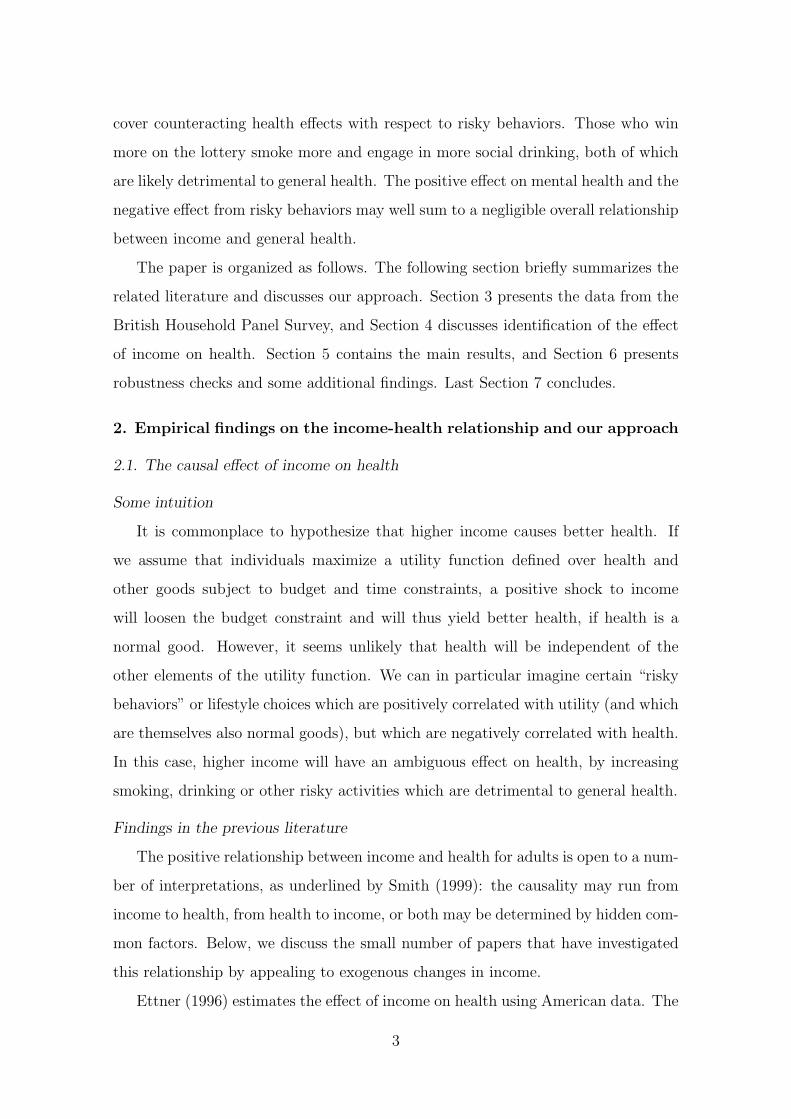
Mental health

To measure mental health, we use a score calculated from the General Health

Questionnaire (GHQ). This latter is widely-used by psychologists, epidemiologists

and medical researchers as an indicator of mental functioning. The BHPS contains

the 12-item version of the GHQ, based on the following questions. BHPS respon-

dents are asked:

“Here are some questions regarding the way you have been feeling over

the last few weeks. For each question please ring the number next to the

answer that best suits the way you have felt. Have you recently....

a) been able to concentrate on whatever you’re doing?b) lost much sleep over worry?c) felt that you were playing a useful part in things?d) felt capable of making decisions about things?e) felt constantly under strain?f) felt you couldn’t overcome your difficulties?g) been able to enjoy your normal day-to-day activities?h) been able to face up to problems?i) been feeling unhappy or depressed?j) been losing confidence in yourself?k) been thinking of yourself as a worthless person?l) been feeling reasonably happy, all things considered?”

Question a) is answered on the following four-point scale:

1: Better than usual2: Same as usual3: Less than usual4: Much less than usual

8

Questions b), e), f), i), j) and k) are answered as follows:

1: Not at all2: No more than usual3: Rather more than usual4: Much more than usual

And the replies to questions c), d), g), h) and l) are on the following scale:

1: More so than usual2: About same as usual3: Less so than usual4: Much less than usual

The main mental health variable used in this paper is the Caseness GHQ score,

which counts the number of questions for which the response is in one of the two “low

well-being” categories. This count is then reversed so that higher scores indicate

higher levels of well-being, running from 0 (all twelve responses indicating poor

psychological health) to 12 (no responses indicating poor psychological health).3

Physical health - Health problems

The data also contain a number of variables indicating the presence of specific

health problems. Amongst these, we retain only those which describe specific phys-

ical problems. These refer to:4

1) Arms, legs, hands, etc2) Sight3) Hearing4) Skin conditions/allergy5) Chest/breathing6) Heart/blood pressure7) Stomach or digestion8) Diabetes.

Physical health - Behaviors

We consider two separate risky behaviors: smoking and drinking. We have

two distinct smoking variables. The first is a binary variable showing whether the

3GHQ information from the BHPS has been used by Economists in a number of differentcontexts: see Clark and Oswald (1994), Clark (2003), Ermisch et al. (2004), Gardner and Oswald(2007), and Powdthavee (2009).

4The BHPS also asks about health problems with respect to Alcohol and Drugs, and Epilepsy.We do not analyze these two variables as few respondents report such problems.

9

respondent is a “current smoker” or not. This variable is called “Smoker”. Our

second variable called “Cig” indicates the number of cigarettes the individual smokes

per day. We recode this number using the following scale:

1: Between 1 and 10 cigarettes per day2: Between 11 and 15 cigarettes per day3: Between 16 and 30 cigarettes per day4: More than 30 cigarettes per day

Drinking is measured via an ordinal variable (“Drink”) which indicates the fre-

quency with which the respondent goes for a drink at a pub or club. This variable

is coded as follows, where higher values indicate more social drinking:

1: Never/almost never2: Once a year or less3: Several times a year4: At least once a month5: At least once a week

Figures 1 and 2 show the distribution of these six health variables. The median

and the mode of self-assessed health is “Good”, and the GHQ score exhibits strong

right skew. Around one-quarter of BHPS respondents are current smokers, and the

modal category for social drinking is “At least once a week”, although almost twenty

percent never go out to pubs or clubs.

Lottery wins

We are interested in the relationship between income and these different health

measures. To try to identify a causal relationship between income and health, we

appeal to two BHPS questions on lottery wins as a source of exogenous changes in

income. These have appeared every year from 1997 onwards, and are worded as

follows:

“Since September 1st (year before) have you received any payments, or

payment in kind, from a win on the football pools, national lottery or

other form of gambling?”

10

If this question was answered in the positive, then the respondent was asked:

“About how much in total did you receive? (win on the football pools,

national lottery or other form of gambling)”

As such, we know both whether the individual won, and how much in total they

received. The average win reported, expressed in real 2005 Pounds, is around £170.

Five per cent of winners win more than £500, and the largest win is over £140 000.

However, one potential weakness of the lottery data in the BHPS5 is that it

does not contain any direct information about the number of times (if any) that the

individual has played the lottery. As such, we cannot distinguish non-players from

unsuccessful players. A second point is that, both for lottery winners and playing

non-winners, we do not know how much has been gambled.

On the other hand, there are significant advantages in using lottery winnings.

Firstly, as noted previously, we can consider their receipt as being largely exogenous.

Second, in Britain, as opposed to a number of other countries, many people play lot-

teries. A recent survey-based estimate (Wardle et al., 2007) is that over two-thirds

of the British participate in some kind of gambling in a given year, with 57% of the

population playing the National Lottery (and almost 60% of the latter playing at

least once a week). The Camelot Group, who are the current National Lottery opera-

tors, report that just under £5 Billion was spent on the lottery in the year 2007-2008

(http://www.camelotgroup.co.uk/aboutcamelot/annualreports/2008AnnualReport

.html). Consequently, there are a considerable number of lottery winners in the

BHPS data.

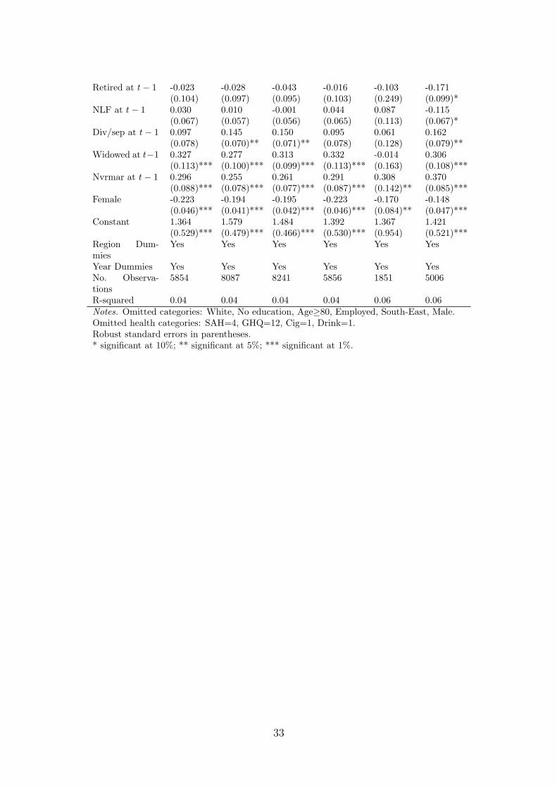
Lottery winnings are adjusted for inflation via the consumer price index (see

Table 3) and are expressed in 2005 Pounds. In the empirical analysis, we will use

the logarithm of lottery winnings, partly as income is very often entered in log form

in the empirical analysis of health and well-being, and partly because the distribution

of lottery winnings is, unsurprisingly, extremely right-skewed.6 The distribution of

5Which weakness also appears in the Swedish lottery data used by Lindahl (2002), but notin the analysis of Kuhn et al. (2008), who are able to control for the number of lottery ticketspurchased.

6Experiments using a set of lottery-winnings dummies consistently produced qualitatively sim-ilar results to those using log of the prize.

11

the log of lottery winnings for winners is shown in Figure 3.

4. Identifying Exogenous Income Effects

Section 3 above highlighted the exogenous income variables that are available in

the BHPS. However, the way in which lottery winnings should be used in a causal

regression framework merits some reflection. The underlying issue is that, while we

suppose that winning the lottery is a random event, conditional on having played,

the actual fact of playing the lottery may well itself be endogenous: non-players and

players are likely to differ in both their observable and unobservable characteristics.

As noted above, the BHPS does not include information on whether individuals play

the lottery or not: we cannot distinguish players from non-players, only winners from

non-winners.

Winners versus Non-Winners

One simple way of using lottery-winnings information would be to compare the

health of those who have not won the lottery (which group consists of both non-

players and unlucky players) to the health of winners. However, these two groups

are not likely to be comparable, as the decision to play the lottery is probably

endogenous, which poses serious problems for the interpretation of the coefficient on

lottery winnings.

This phenomenon is illustrated in the Venn diagram in Figure 4. The first,

larger, set consists of those who play the lottery. These players likely have different

characteristics, both observed and unobserved, to non-players. The key issue in

the BHPS data (which we believe is common to many datasets covering lottery

winnings) is that this distinction between those who play and those who do not play

is unobserved (which is why we have drawn the frontier of this set as a broken line).

There is a second set, entirely contained within the first: this is the set of winners,

all of whom by definition are players. This is the frontier that we do observe (which

is represented as an unbroken line).

While the group of winners in Figure 4 might be fairly homogeneous (we will

test this explicitly below), amongst non-winners we have both those who did not

play, and those who did play but did not win. If playing the lottery is endogenous,

12

individual characteristics will differ between the groups. It can of course be argued

that we can condition on any observable differences, once we have identified them.

However, non-players and players (and therefore non-winners and winners) may also

differ fundamentally in other unobservable ways. For example, non-players (who are

included in the group of non-winners) may well be more risk-averse, and as a result

invest more in their own health capital. This seriously flaws any comparison of

health between winners and non-winners: as such we do not compare these two

groups in our analysis.

To illustrate this potential bias, we create a dummy variable for having won the

lottery (called “Win”), and regress it on a number of individual characteristics:

Winit = F (α + βhit−1 + γxit−1)

where hit−1 represents health at date t− 1 and xit−1 denotes the other control vari-

ables, including income.7 The function F here is the cumulative normal distribution,

and we estimate this equation as a simple probit.

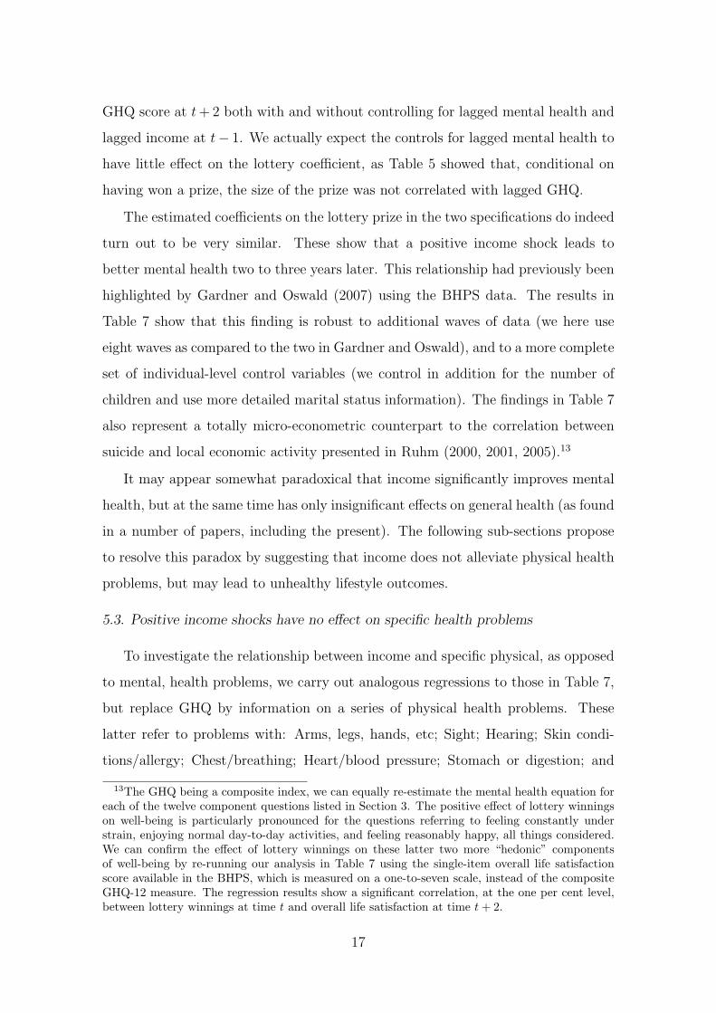
Table 4 presents the regression results. These show that the probability of win-

ning the lottery is significantly correlated with lagged income, ethnicity, education,

labor-market status, number of children and age. It is also correlated with four of

the lagged physical health problem variables (those in worse health are more likely

to win, and thus, we suggest, are more likely to play the lottery). 8 The results in

Table 4 hence underline that those who win and those who do not win differ in a

number of observable ways, and thus we suggest likely differ in unobservables too.

To overcome this problem, the remainder of the paper concentrates on the health

outcomes of big compared to small lottery winners.

7The non-lottery income variable that we use in this regression, and in our health and well-being regressions, is called “hhnyrde”, a derived variable supplied with the BHPS, which measurestotal household annual income, equivalized using the McClements before housing costs scale, andadjusted for the prices of the reference month.

8One dataset that does contain information on whether people played or not is the UK FamilyExpenditure Survey. Analysis of three cross-sectional waves of this data from 1998/1999, 1999/2000and 2000/2001 shows that the probability of playing the lottery is related to standard individualdemographics in very much the same way as the probability of winning in Table 4. The fact thatthe FES is not panel, and does not include health information, however renders it inapt for thequestion we analyze here

13

Big versus Small Winners

The exogenous effect of income amongst winners is identified from the compar-

ison of those who have won larger amounts of money to those who won smaller

amounts. This distinction is arguably far more exogenous (although it may still

depend on how much individuals play). To show that there is less of an endogeneity

problem here, we regress the amount won (for winners only) on the same right-hand

side variables as previously used in Table 4:

Log(Prize)it = α + βhit−1 + γxit−1 + εit

Table 5 shows the results of this OLS regression. Fewer of the individual variables

are correlated with the amount won. The populations of large and small winners

seem to be similar according to labor market status and age, which was not the case

in Table 4. This relative similarity in observables leads us to suspect a corresponding

similarity in unobservables, and it is on this basis that we will evaluate the effect of

income on health.

5. The Effect of Income on Health Outcomes

In line with the existing literature, our health regressions include a number of

fairly standard explanatory variables: age, ethnicity, education, labor-market and

marital status, number of children, region and wave. We examine the effect of in-

come on the different health outcomes listed above: self-assessed health, physical

health problems, mental health, and smoking and drinking. Our key right-hand

side variable is exogenous income from the comparison of large and small lottery

winnings. For notation purposes, we consider lottery winnings that are reported in

year t (for example, someone interviewed in Wave 10, say in October 2000, reports

any lottery winnings between September 1999 and the date of their Wave 10 inter-

view). To evaluate the effect of such winnings on health, we imagine that any health

investments may take time to bear fruit, and consider health at date t + 2 as our

dependent variable (to continue the example above, we will consider health at Wave

12, that is between two to three years after the lottery win).9 Further, as is fairly

9Oswald and Winkelmann (2008) also find a delayed effect of lottery winnings on a measure

14

common in this literature, some of the regressions will control for the individual’s

lagged health status at t− 1.10

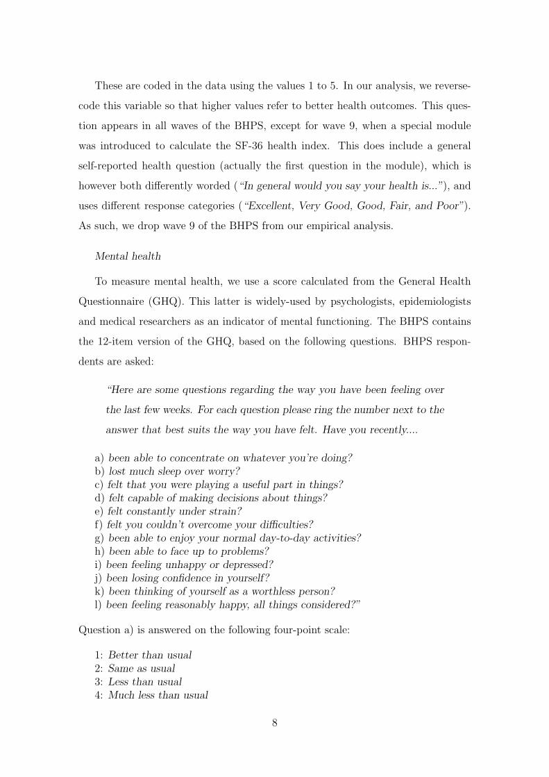
The model below examines the average effect of lottery winnings on different

types of health. For all health variables except social drinking, we use the following

model:

hit+2 = F (α + β.Log(Prize)it + γ2.xit+2)

Here hit+2 is health at time t + 2. Because of data availability11 we are obliged to

replace hit+2 with hit+1 when looking at the effect of lottery prizes on social drinking:

hit+1 = F (α + β.Log(Prize)it + γ2.xit+1)

In both of the above models t is the year of the lottery win and the x are the other

control variables. The health equations are estimated via ordered probits or probits.

In order to allow for correlation between errors for repeated observations on the

same individual, we cluster standard errors at the individual level.

The following sub-sections discuss the estimation results for our different health

variables in turn.

5.1. General health status

The regression results for the most general of our dependent variables, self-

assessed health, appear in Table 6. This table shows the effect of lottery winnings

reported at t on self-assessed health at t+2. There are two columns in this table. The

of well-being. They use GSOEP data to show that financial satisfaction is significantly positivelycorrelated with the amount won by lottery winners, but only three years after the win. Thereis no significant effect one or two years after a win. They interpret their results as indicatingdeservingness: individuals only enjoy their winnings when they feel that they have deserved them.Deservingness is endogenous and can be created by the individual, but this costly investment takestime, which explains the lack of any significant effect immediately following the win. Equally,Kuhn et al. (2008) find no effect of the amount won in the Dutch postcode lottery on individualhappiness six months later.

10In the context of completely exogenous movements in income, controls for lagged health arenot necessary. When lottery prizes are distributed randomly, then controlling for lagged health willnot affect the estimated coefficient on lottery winnings in a health equation. We believe that thesize of lottery wins (amongst winners) is fairly random; the regression results in Table 5 supportthis reading. In practical terms, the presence or absence of lagged health in our regressions mostoften makes little qualitative difference to the estimated coefficient on lottery winnings.

11Social drinking is only recorded every two years in the BHPS. As we sometimes condition onone-year lags in the health variable under consideration, we are not able to estimate a drinkingequation with terms in both t− 1 and t + 2.

15

first reproduces the health specification described in the first equation above. The

second adds both lagged self-assessed health and log equivalent household income,

measured at t− 1.12

The main coefficients of interest here are those on the log prize variables: these

are positive but insignificant, and provide no evidence that exogenous income im-

proves general health. This is consistent with previous results in Meer et al. (2003).

It is worth underlining that this table does indeed show a social gradient in health:

the significant estimate on log income at the end of the table tells us that individ-

uals with higher incomes are in better health. The fact that lottery winnings do

not affect health then leads us to suspect that the relationship between income and

health is not causal in this direction: either health causes income, or both reflect

some other omitted variable such as the quality of the maternal diet, or the type of

school the individual attended.

A number of the other right-hand side variables in column (2) (which are not

shown in Table 6 for space reasons) attract only insignificant coefficients. This is

due to the fact that many of them move only little over time, and as such are picked

up by the four lagged health dummies (we exclude health category 4, corresponding

to “good health”, as this is the largest category).

It is likely that self-assessed health reflect both physical and mental elements.

Following the well-known macro work of Ruhm (2000), it is possible that these move

in opposite directions to produce an insignificant net effect of “better economic

conditions” (i.e. higher income) at the individual level. With this distinction in

mind, we now appeal to the separate measures detailed in Section 3 above to see

whether physical and mental health do indeed have sharply different relationships

with exogenous income. In line with Ruhm’s results, we will pay particular attention

to health behaviors.

5.2. Positive income shocks improve mental health

The results for mental health are shown in Table 7. There are two columns in this

table. These show the relationship between lottery winnings at t and the individual’s

12We do this in particular as there is some evidence in Table 5 that individuals in richer house-holds win larger lottery prizes.

16

GHQ score at t + 2 both with and without controlling for lagged mental health and

lagged income at t− 1. We actually expect the controls for lagged mental health to

have little effect on the lottery coefficient, as Table 5 showed that, conditional on

having won a prize, the size of the prize was not correlated with lagged GHQ.

The estimated coefficients on the lottery prize in the two specifications do indeed

turn out to be very similar. These show that a positive income shock leads to

better mental health two to three years later. This relationship had previously been

highlighted by Gardner and Oswald (2007) using the BHPS data. The results in

Table 7 show that this finding is robust to additional waves of data (we here use

eight waves as compared to the two in Gardner and Oswald), and to a more complete

set of individual-level control variables (we control in addition for the number of

children and use more detailed marital status information). The findings in Table 7

also represent a totally micro-econometric counterpart to the correlation between

suicide and local economic activity presented in Ruhm (2000, 2001, 2005).13

It may appear somewhat paradoxical that income significantly improves mental

health, but at the same time has only insignificant effects on general health (as found

in a number of papers, including the present). The following sub-sections propose

to resolve this paradox by suggesting that income does not alleviate physical health

problems, but may lead to unhealthy lifestyle outcomes.

5.3. Positive income shocks have no effect on specific health problems

To investigate the relationship between income and specific physical, as opposed

to mental, health problems, we carry out analogous regressions to those in Table 7,

but replace GHQ by information on a series of physical health problems. These

latter refer to problems with: Arms, legs, hands, etc; Sight; Hearing; Skin condi-

tions/allergy; Chest/breathing; Heart/blood pressure; Stomach or digestion; and

13The GHQ being a composite index, we can equally re-estimate the mental health equation foreach of the twelve component questions listed in Section 3. The positive effect of lottery winningson well-being is particularly pronounced for the questions referring to feeling constantly understrain, enjoying normal day-to-day activities, and feeling reasonably happy, all things considered.We can confirm the effect of lottery winnings on these latter two more “hedonic” componentsof well-being by re-running our analysis in Table 7 using the single-item overall life satisfactionscore available in the BHPS, which is measured on a one-to-seven scale, instead of the compositeGHQ-12 measure. The regression results show a significant correlation, at the one per cent level,between lottery winnings at time t and overall life satisfaction at time t + 2.

17

Diabetes. All of these problems are evaluated at t+2, whereas the lottery prize was

reported at t.

We carried out the analysis for each of the above eight problems separately. The

regression results (available on request) systematically show no relationship between

lottery winnings and these physical health problems. This might be argued to be

unsurprising: higher income may well not improve individuals’ sight, hearing, or

skin conditions. However, one area where income might play a larger role is in the

specific behaviors that individuals undertake (i.e. the way in which they live their

lives), and their ensuing health effects. In the following, we specifically consider the

relationship between lottery winnings, smoking and social drinking.

5.4. Positive income shocks lead to worse lifestyles

The hypothesis we test in this last sub-section is that positive individual income

shocks may have a detrimental effect on physical health via individual lifestyles. In

what follows, we specifically consider smoking and drinking.

Around 25% of our estimation sample of lottery winners report being current

smokers. Columns (1) and (2) of Table 8 model the probability that the individual

be a smoker. The demographic control variables here (not shown) are the same

as in Table 7. We are most interested in the effect of lottery winnings on smoking.

The first line of Table 8 reveals that positive income shocks (which occurred between

t−1 and t) significantly increase the probability of smoking at t+2. Providing more

detail on the smoking decision, columns (3) and (4) suggest that lottery winnings

increase the probability of smoking a greater number of cigarettes.14

In columns (5) and (6) we repeat this exercise for the one measure of social

drinking that is available in the BHPS: a categorical variable for the frequency of

going out for a drink at a pub or club. The results are qualitatively the same as

in columns (1) - (4): the greater is the lottery prize, the greater the probability of

14Column (3) is an ordered probit of the four classes of cigarette consumption at t+2, describedin Section 3, regressed on log winnings at time t and the other explanatory variables at timet + 2. Current (t + 2) non-smokers are thus dropped from this analysis. Column (4) is also anordered probit of current cigarette consumption, which controls in addition for the t− 1 values ofhousehold equivalent income and cigarette consumption. As this latter is only defined for smokers,the regression sample in column (4) consists of continuing smokers between t− 1 and t + 2.

18

more frequent social drinking.15

Table 8 therefore shows that, rather than producing better health, higher in-

come is also associated with increased behaviors that are commonly thought to

be unhealthy. Much work has shown that, in general, higher income is associated

with more favorable health outcomes. Our results here nuance this empirical fact.

Positive individual income shocks produce changes in lifestyles which may well be

prejudicial to health. This is entirely consistent with Ruhm (2000, 2001, 2005),

who considers the relationship between risky health behaviors and economic booms.

Ruhm’s approach is very similar to ours at one level: by relating individual (and

aggregate) health outcomes to local labor market conditions, he is able to appeal to

the exogeneity of the latter in determining individual health. Our results above can

be read as the micro-econometric analogy of those in Ruhm. At the individual level

also, exogenously higher income produces unhealthy living.

The correlations revealed by these exogenous movements are therefore largely

contradictory to the commonly-noted positive link between health and social status.

In reality positive (exogenous) income shocks seem to lead to lifestyle choices which

are associated with worse health outcomes.16

6. Robustness Checks and Additional Findings

6.1. Net or Gross Winnings?

The BHPS question on lottery winnings asks individuals to report “about how

much in total did you receive”. Although it is not made explicit, the most likely

interpretation of this question is in terms of gross winnings. Playing the lottery

15We can calculate the marginal effect of lottery winnings on different types of outcomes. Theseprobabilities are calculated for an individual with characteristics that are fairly representative inour sample of winners. We evaluate the effect of winning £10 000, as opposed to the mean amountwon of £170. The marginal effect of these higher winnings on GHQ, from Table 7, is of a fourpercentage point rise in the probability of reporting the highest mental well-being score (i.e. 12).The same method applied to the results in Table 8 produces another four percentage point increasein the probability of being in the top social drinking category (at least once a week), and a riseof eight percentage points in the probability of increasing the number of cigarettes smoked (giventhat the person was a light smoker - 1 to 10 a day - before winning the lottery).

16This is arguably also reflected in hospital attendance. The BHPS asks all respondents “approx-imately how many times have you attended a hospital or clinic as an out-patient or day patient?”,with answers on a five-point ordered scale. Using this variable as a health outcome, in the sameway as in Table 8, produces some evidence of a positive correlation with the log of the lotteryprize: winners end up going to the hospital more often.

19

costs money, and it is possible that some of our winners could have actually spent

more on lottery tickets over the year than they ended up winning. In general, net

winnings will be smaller than gross winnings. We are interested here in the effect

of an individual’s financial resources on their health and well-being. Our measure

of (gross) lottery winnings then overstates the movement in the resources that they

have available to them. As such, our estimated coefficient on lottery winnings is

actually biased downwards. To explore this matter further, we re-estimated Tables

6-8, introducing not only the amount of the lottery win, but also an interaction

between winnings and the fact of winning at least £1000 (we imagine that with

gross winnings of at least this amount were considerably less likely to be net losers).

None of the coefficients on these interactions were close to significant, leading us to

suspect that our main health results are robust.

6.2. Household or Individual Income?

Although it is not the main focus of our paper, we have controlled for (lagged)

household equivalent income in some of our regressions (even though the results

are often only little changed in this specification). One potential question that can

be asked is whether we should use an income measure that picks up the outcomes

for other household members, when we have specifically concentrated on lottery

winnings at the individual level. To investigate, we have re-estimated all of our

analysis tables using a measure of the individual’s own annual income (in real terms).

The results, in terms of the significance level of the log winnings variable, were not

affected.17

6.3. Frequent Social Drinking

Our analysis of the endogeneity of lottery winnings in Table 5 led to the broad

conclusion that health at t−1 did not predict the amount won on the lottery at date t.

One very significant exception to this rule appears in column (6) of that table, where

the most frequent social drinkers at t − 1 systematically win more on the lottery.

This raises the possibility that “big winners” are different in some unobservable

way from little winners, and that these unobserved variables are correlated with

17Equally, entering lottery winnings deflated using an equivalence scale does not change theresults

20

health outcomes. To check whether the most frequent social drinkers were behind

the significant lottery winning coefficient in Table 8, columns (5) and (6), we drop

those in the top social drinking category at date t − 1. The qualitative results are

unchanged, with the estimated coefficients on lottery winnings remaining significant

with t-statistics of over two.

6.4. Sub-regressions

All of the results to date have concerned the entire sample of lottery winners.

Despite the danger of ending up with only a relatively small sample, we have also

run the same analyses on various sub-groups of the data. A first split is according

to mean income. There is no SAH effect in either group, but we do note a stronger

GHQ effect for those with lower income, and an effect on smoking that appears to

be stronger for those with higher income. A separate analysis by age (splitting at

the age of 45) reveals a stronger SAH and GHQ effect for older than for younger

respondents, while the effect on social drinking is stronger for younger respondents.

Last, there is no sharp difference in the shape of the results for men and for women.18

7. Conclusion

This paper has asked whether money makes individuals healthier. While it seems

well-known that the rich enjoy better health, it is far more difficult to establish the

causality of this relationship. A small recent literature has appealed to exogenous

movements in income, for example lottery winnings and inheritances, to reveal either

small or negligible effects of income on general health. At the same time, lottery

winnings have been shown to produce better mental health.

We have suggested resolving this apparent paradox by appealing to an entirely

individual-level analogy of the well-known work of Ruhm (2000, 2001, 2005), and

distinguishing between physical and mental health. Ruhm showed that recessions

are associated with healthier living but more suicides. Using a sample of lottery

winners only, “better economic conditions”, which at our micro level are picked up

18Inspired by some of the results in Miller (2009), we equally considered the effects of lottery win-nings according to labor-market attachment. Consistent with their results, we find a systematicallylarger well-being effect for the unemployed and inactive, compared to the employed. However,theresults with respect to health behaviors are more mixed, with some evidence of a greater drinkingand smoking effect amongst the employed

21

by greater lottery winnings, produce higher GHQ mental health scores, but also a

greater likelihood of smoking and social drinking.

The results presented here have more generally underlined three arguably central

points in the analysis of health outcomes. The first is that it is unlikely that income

is exogenous, so that instrumentation is essential for the understanding of causal

relationships. Second, health is not a holistic concept, and we need to both be clear

about what kind of health we are talking about, and be ready for the possibility

that different types of health behave in very different ways. Last, the comparison

of results from different levels of aggregation of both dependent and explanatory

variables is a fruitful avenue of research in the economics of health and well-being.

22

References

Adda, J., Banks, J., von Gaudecker, H.-M., 2009. The Impact of Income Shockson Health: Evidence from Cohort Data. Journal of the European EconomicAssociation, 7, 6, 1361-1399.

Bodkin, R., 1959. Windfall Income and Consumption. American Economic Re-view, 49, 4, 602-614.

Brickman, P.D.C., Janoff-Bulman, R., 1978. Lottery winners and accident victims:Is happiness relative? Journal of Personality and Social Psychology, 36, 917-927.

Clark, A.E., 2003. Unemployment as a Social Norm: Psychological Evidence fromPanel Data. Journal of Labor Economics, 21, 323-351.

Clark, A.E., Oswald, A.J., 1994. Unhappiness and Unemployment. EconomicJournal, 104, 648-659.

Deaton, A.S., Paxson, C.H., 1999. Mortality, Education, Income, and Inequalityamong American Cohorts. NBER Working Paper No. W7140.

Ermisch, J., Francesconi, M., Pevalin, D.J., 2004. Parental partnership and job-lessness in childhood and their influence on young people’s outcomes. Journalof the Royal Statistical Society Series A, 167, 1, 69-101.

Ettner, S., 1996. New Evidence on the Relationship Between Income and Health.Journal of Health Economics, 15, 1, 67-86.

Frijters, P., Haisken-DeNew, J.P., Shields, M.A., 2005. The Causal Effect of In-come on Health: Evidence from German Reunification. Journal of HealthEconomics, 24, 5, 997-1017.

Gardner, J., Oswald, A., 2007. Money and Mental Wellbeing: A LongitudinalStudy of Medium-sized Lottery Wins. Journal of Health Economics, 26, 1,49-60.

Henley, A., 2004. House Price Shocks, Windfall Gains and Hours of Work: BritishEvidence. Oxford Bulletin of Economics and Statistics, 66, 4, 439-456.

Imbens, G., Rubin, D., Sacerdote, B., 2001. Estimating the Effect of Unearned In-come on Labor Earnings, Savings, and Consumption: Evidence from a Surveyof Lottery Players. American Economic Review, 91, 4, 778-794.

Kuhn, P., Kooreman, P., Soetevent, A., Kapteyn, A., 2008. The Own and SocialEffects of an Unexpected Income Shock. Evidence from the Dutch PostcodeLottery. RAND Working Paper 574.

23

Lindahl, M., 2005. Estimating the Effect of Income on Health Using Lottery Prizesas Exogenous Source of Variation in Income. Journal of Human Resources,40, 1, 144-168.

Lindh, T., Ohlsson, H., 1996. Self-Employment and Windfall Gains: Evidencefrom the Swedish Lottery. Economic Journal, 106, 1515-1526.

Marmot, M., 2004. Status Syndrome. London: Bloomsbury.

Marmot, M., Bobak, M., 2000. International comparators and poverty and healthin Europe. British Medical Journal, 321, 1124-1128.

Meer, J., Miller, D.L., Rosen H.S., 2003. Exploring the Health-Wealth Nexus.Journal of Health Economics, 22, 5, 713-730.

Miller, D., Page, M., Stevens, A., Filipski, M., 2009. Why Are Recessions Goodfor Your Health?. American Economic Review, 99, 2, 122-127.

Oswald, A.J., Winkelmann, R., 2008. Delay and Deservingness after Winning theLottery. University of Zurich Socieconomic Institute, Mimeo.

Powdthavee, N., 2009. Ill-Health as a Social Norm: Evidence from Other People’sHealth Problems. Social Science and Medicine, 68, 251-259.

Ruhm, C., 2000. Are Recessions Good for your Health? Quarterly Journal ofEconomics, 115, 2, 617-650.

Ruhm, C., 2001. Economic Expansions are Unhealthy. Evidence from Microdata.NBER Working Paper, 8447.

Ruhm, C., 2005. Healthy Living in Hard Times. Journal of Health Economics, 24,2, 341-363.

Taylor, M.P., 2001. Self-Employment and Windfall Gains in Britain: Evidencefrom Panel Data. Economica, 68, 539-565.

Smith, J., 1999. Healthy Bodies and Thick Wallets: The Dual Relation betweenHealth and Economic Status. Journal of Economic Perspectives, 13, 145-166.

Van Doorslaer, E., Wagstaff, A., Bleichrodt, H., Calonge, S., Gerdtham, U., Gerfin,M., Geurts, J., Gross, L., Hakkinen, U., Leu, R.E., O’Donell, O., Propper,C., Puffer, F., Rodriguez, M., Sundberg, G., Winkelhake, O., 1997. Income-related inequalities in health: some international comparisons. Journal ofHealth Economics, 16, 1, 93-112.

Wardle, H., Sproston, K., Orford, J., Erens, B., Griffiths, M. Constantine, R.,Pigott, S., 2007. British Gambling Prevalence Survey 2007, National Centrefor Social Research.

Winkleby, M.A., Jatulis, D.E., Frank, E., Fortmann, S.P., 1992. Socioeconomicstatus and health: how education, income, and occupation contribute to riskfactors for cardiovascular disease. American Journal of Public Health, 82,816-820.

24

Table 1: Findings in the literature

General health Mental healthGeneral SAH

Health ScoreEttner (1996) + +

(Scale ofdepressive symptoms)

Lindahl (2002) +Meer et al. (2003) nsFrijters et al. (2005) +

(very small)Gardner and Oswald (2007) +

(GHQ)Note: “+” stands for a “positive and significant effect of income on the health scorein question” and “ns” stands for “no significant effect”.

25

Table 2: Definition of analysis variables

HealthGeneral healthSAH =1 if poor health

to =5 if excellent health

Mental healthGHQ =0 for worst mental health

to =12 for best mental health

Physical healthHealth Pb X =1 if reports health problem XSmoker =1 if the individual smokesCig =1 if the individual smokes between 1 and 10 cigarettes per day

to =4 if the individual smokes more than 30 cigarettes per dayDrink =1 if never or almost never goes out for a drink to a pub or club

to =5 if goes out for a drink to a pub or club at least once a week

LotteryWint =0 if the individual does not win at date t

=1 if the individual wins at date tLog(Prize) Logarithm of lottery prize

Control variablesLog(inc) Logarithm of income (real annual household income, equivalized using the McClements scale)White ReferenceNon-white =1 if not whiteNo. children Number of children in the householdNo education ReferenceO-levels =1 if has O-levelsA-levels =1 if has A-levelsHND, HNC =1 if has a College degreeDegree =1 if has a University degreeEmployed ReferenceUnemp =1 if unemployedRetired =1 if retiredNLF =1 if not in the labor forceMarried ReferenceDivsep =1 if separated or divorcedWidowed =1 if widowedNvrmar =1 if never marriedAge Dummy variables for age groups:

16-19, 20-24, 25-29, 30-34,.... 75-79, 80+Region Dummy variables for each regionYear Dummy variables for each year

26

Table 3: The consumer price index for the UKYear 1997 1998 1999 2000 2001 2002 2003 2004 2005CPI 89.7 91.1 92.3 93.1 94.2 95.4 96.7 98.0 100.0Source. http://www.statistics.gov.uk/statbase/TSDdownload2.asp

27

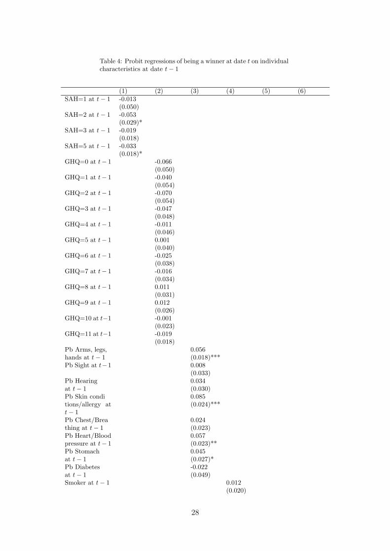
Table 4: Probit regressions of being a winner at date t on individualcharacteristics at date t− 1

(1) (2) (3) (4) (5) (6)SAH=1 at t− 1 -0.013

(0.050)SAH=2 at t− 1 -0.053

(0.029)*SAH=3 at t− 1 -0.019

(0.018)SAH=5 at t− 1 -0.033

(0.018)*GHQ=0 at t− 1 -0.066

(0.050)GHQ=1 at t− 1 -0.040

(0.054)GHQ=2 at t− 1 -0.070

(0.054)GHQ=3 at t− 1 -0.047

(0.048)GHQ=4 at t− 1 -0.011

(0.046)GHQ=5 at t− 1 0.001

(0.040)GHQ=6 at t− 1 -0.025

(0.038)GHQ=7 at t− 1 -0.016

(0.034)GHQ=8 at t− 1 0.011

(0.031)GHQ=9 at t− 1 0.012

(0.026)GHQ=10 at t−1 -0.001

(0.023)GHQ=11 at t−1 -0.019

(0.018)Pb Arms, legs, 0.056hands at t− 1 (0.018)***Pb Sight at t−1 0.008

(0.033)Pb Hearing 0.034at t− 1 (0.030)Pb Skin condi 0.085tions/allergy att− 1

(0.024)***

Pb Chest/Brea 0.024thing at t− 1 (0.023)Pb Heart/Blood 0.057pressure at t− 1 (0.023)**Pb Stomach 0.045at t− 1 (0.027)*Pb Diabetes -0.022at t− 1 (0.049)Smoker at t− 1 0.012

(0.020)

28

Cig=2 at t− 1 0.088(0.036)**

Cig=3 at t− 1 0.087(0.034)**

Cig=4 at t− 1 0.063(0.093)

Drink=2 at t−1 -0.009(0.038)

Drink=3 at t−1 0.097(0.029)***

Drink=4 at t−1 0.082(0.030)***

Drink=5 at t−1 0.154(0.029)***

Log(inc) at t− 1 0.104 0.102 0.105 0.106 0.146 0.105(0.015)*** (0.014)*** (0.014)*** (0.015)*** (0.027)*** (0.017)***

Non-white -0.356 -0.370 -0.379 -0.355 -0.287 -0.275(0.068)*** (0.069)*** (0.067)*** (0.068)*** (0.105)*** (0.067)***

No. children -0.067 -0.058 -0.056 -0.067 -0.082 -0.058at t− 1 (0.012)*** (0.011)*** (0.011)*** (0.012)*** (0.020)*** (0.013)***O-levels at t− 1 0.063 0.055 0.062 0.066 0.095 0.061

(0.025)** (0.025)** (0.025)** (0.025)*** (0.042)** (0.027)**A-levels at t− 1 0.004 0.007 0.012 0.007 0.027 0.016

(0.028) (0.027) (0.027) (0.028) (0.048) (0.030)HND, HNC -0.080 -0.092 -0.085 -0.077 -0.002 -0.099at t− 1 (0.039)** (0.038)** (0.038)** (0.039)** (0.075) (0.042)**Degree at t− 1 -0.239 -0.244 -0.237 -0.236 -0.226 -0.241

(0.035)*** (0.035)*** (0.035)*** (0.036)*** (0.078)*** (0.038)***16-19 at t− 1 0.093 0.060 0.135 0.090 0.041 -0.010

(0.075) (0.074) (0.074)* (0.075) (0.174) (0.085)20-24 at t− 1 0.184 0.143 0.204 0.178 0.140 0.082

(0.072)** (0.071)** (0.071)*** (0.072)** (0.169) (0.082)25-29 at t− 1 0.183 0.134 0.189 0.176 0.071 0.129

(0.069)*** (0.069)* (0.069)*** (0.070)** (0.167) (0.079)30-34 at t− 1 0.223 0.193 0.243 0.216 0.121 0.153

(0.069)*** (0.068)*** (0.068)*** (0.069)*** (0.166) (0.078)**35-39 at t− 1 0.285 0.260 0.302 0.278 0.188 0.268

(0.069)*** (0.068)*** (0.067)*** (0.069)*** (0.166) (0.077)***40-44 at t− 1 0.266 0.240 0.283 0.261 0.152 0.205

(0.068)*** (0.068)*** (0.067)*** (0.069)*** (0.166) (0.077)***45-49 at t− 1 0.249 0.232 0.268 0.243 0.155 0.204

(0.067)*** (0.067)*** (0.066)*** (0.068)*** (0.164) (0.076)***50-54 at t− 1 0.253 0.228 0.263 0.248 0.138 0.221

(0.066)*** (0.065)*** (0.064)*** (0.066)*** (0.161) (0.074)***55-59 at t− 1 0.217 0.188 0.219 0.213 0.027 0.197

(0.064)*** (0.064)*** (0.063)*** (0.064)*** (0.160) (0.073)***60-64 at t− 1 0.162 0.143 0.170 0.159 0.068 0.141

(0.062)*** (0.061)** (0.060)*** (0.062)** (0.156) (0.070)**65-69 at t− 1 0.203 0.199 0.222 0.200 0.176 0.188

(0.060)*** (0.060)*** (0.059)*** (0.060)*** (0.154) (0.067)***70-74 at t− 1 0.117 0.116 0.128 0.116 -0.016 0.081

(0.059)** (0.059)* (0.058)** (0.059)* (0.160) (0.067)75-79 at t− 1 0.027 0.001 0.018 0.026 -0.056 -0.022

(0.059) (0.059) (0.058) (0.059) (0.166) (0.069)Unemployed -0.224 -0.195 -0.204 -0.228 -0.213 -0.239at t− 1 (0.047)*** (0.044)*** (0.044)*** (0.047)*** (0.064)*** (0.054)***

29

Retired at t− 1 -0.019 -0.041 -0.056 -0.021 -0.037 0.014(0.035) (0.034) (0.034) (0.035) (0.070) (0.041)

NLF at t− 1 -0.091 -0.096 -0.124 -0.096 -0.037 -0.059(0.025)*** (0.024)*** (0.024)*** (0.024)*** (0.039) (0.027)**

Div/sep at t− 1 -0.072 -0.064 -0.071 -0.075 -0.152 -0.063(0.031)** (0.030)** (0.030)** (0.031)** (0.046)*** (0.033)*

Widowed at t−1 -0.112 -0.105 -0.104 -0.115 -0.131 -0.094(0.039)*** (0.038)*** (0.037)*** (0.039)*** (0.075)* (0.043)**

Nvrmar at t− 1 0.016 0.019 0.016 0.016 -0.066 0.029(0.029) (0.028) (0.028) (0.029) (0.048) (0.031)

Female -0.231 -0.232 -0.235 -0.231 -0.159 -0.221(0.019)*** (0.019)*** (0.018)*** (0.019)*** (0.033)*** (0.021)***

Constant -1.964 -2.106 -2.212 -1.988 -2.288 -2.235(0.163)*** (0.158)*** (0.157)*** (0.163)*** (0.314)*** (0.183)***

Region Dum-mies

Yes Yes Yes Yes Yes Yes

Year Dummies Yes Yes Yes Yes Yes YesNo. Observa-tions

84029 93333 95812 84032 25017 51026

Notes. Omitted categories: White, No education, Age≥80, Employed, South-East, Male.Omitted health categories: SAH=4, GHQ=12, Cig=1, Drink=1.Robust standard errors in parentheses.* significant at 10%; ** significant at 5%; *** significant at 1%.

30

Table 5: OLS regressions of the amount won on the lottery bywinners at date t on individual characteristics at date t− 1

(1) (2) (3) (4) (5) (6)SAH=1 at t− 1 0.002

(0.143)SAH=2 at t− 1 0.074

(0.085)SAH=3 at t− 1 0.095

(0.048)**SAH=5 at t− 1 0.039

(0.050)GHQ=0 at t− 1 -0.137

(0.124)GHQ=1 at t− 1 0.049

(0.148)GHQ=2 at t− 1 -0.083

(0.114)GHQ=3 at t− 1 0.060

(0.118)GHQ=4 at t− 1 -0.199

(0.120)*GHQ=5 at t− 1 0.002

(0.122)GHQ=6 at t− 1 -0.072

(0.089)GHQ=7 at t− 1 -0.157

(0.087)*GHQ=8 at t− 1 -0.148

(0.082)*GHQ=9 at t− 1 -0.016

(0.065)GHQ=10 at t−1 0.056

(0.058)GHQ=11 at t−1 0.030

(0.048)Pb Arms, legs, 0.020hands at t− 1 (0.043)Pb Sight at t−1 -0.153

(0.078)**Pb Hearing 0.072at t− 1 (0.065)Pb Skin condi- -0.000tions/allergy att− 1

(0.059)

Pb Chest/Brea- -0.058thing at t− 1 (0.056)Pb Heart/Blood -0.042pressure at t− 1 (0.055)Pb Stomach 0.073at t− 1 (0.069)Pb Diabetes 0.094at t− 1 (0.139)Smoker at t− 1 0.066

(0.050)

31

Cig=2 at t− 1 0.136(0.097)

Cig=3 at t− 1 0.085(0.091)

Cig=4 at t− 1 0.065(0.225)

Drink=2 at t−1 0.068(0.088)

Drink=3 at t−1 0.011(0.073)

Drink=4 at t−1 0.107(0.077)

Drink=5 at t−1 0.255(0.074)***

Log(inc) at t− 1 0.234 0.215 0.215 0.235 0.259 0.241(0.049)*** (0.044)*** (0.043)*** (0.049)*** (0.079)*** (0.049)***

Non-white -0.398 -0.312 -0.358 -0.399 -0.016 -0.385(0.139)*** (0.133)** (0.127)*** (0.141)*** (0.340) (0.128)***

No. children 0.042 0.039 0.036 0.043 -0.015 0.096at t− 1 (0.034) (0.029) (0.029) (0.034) (0.048) (0.034)***O-levels at t− 1 -0.010 -0.033 -0.035 -0.009 -0.012 -0.046

(0.060) (0.053) (0.053) (0.060) (0.102) (0.061)A-levels at t− 1 -0.046 -0.081 -0.077 -0.037 -0.010 -0.118

(0.069) (0.061) (0.061) (0.069) (0.110) (0.068)*HND, HNC -0.000 -0.023 -0.025 0.001 -0.364 -0.036at t− 1 (0.110) (0.096) (0.096) (0.110) (0.129)*** (0.106)Degree at t− 1 -0.288 -0.326 -0.320 -0.278 -0.475 -0.368

(0.091)*** (0.082)*** (0.082)*** (0.092)*** (0.225)** (0.089)***16-19 at t− 1 -0.381 -0.317 -0.272 -0.398 -0.377 -0.543

(0.219)* (0.214) (0.207) (0.219)* (0.573) (0.222)**20-24 at t− 1 0.046 -0.028 0.022 0.020 -0.269 -0.221

(0.208) (0.207) (0.199) (0.208) (0.560) (0.208)25-29 at t− 1 0.002 0.021 0.049 -0.016 -0.295 -0.123

(0.200) (0.199) (0.191) (0.200) (0.558) (0.197)30-34 at t− 1 -0.019 0.019 0.053 -0.033 -0.167 -0.198

(0.193) (0.195) (0.186) (0.193) (0.553) (0.192)35-39 at t− 1 0.161 0.100 0.125 0.144 -0.081 -0.007

(0.194) (0.195) (0.186) (0.194) (0.553) (0.191)40-44 at t− 1 0.105 0.101 0.133 0.090 -0.046 -0.079

(0.195) (0.195) (0.187) (0.195) (0.562) (0.193)45-49 at t− 1 0.252 0.212 0.239 0.236 0.073 0.143

(0.196) (0.197) (0.188) (0.196) (0.556) (0.191)50-54 at t− 1 0.068 0.021 0.051 0.058 -0.274 -0.021

(0.187) (0.190) (0.179) (0.187) (0.548) (0.183)55-59 at t− 1 0.081 0.044 0.069 0.071 -0.565 0.037

(0.181) (0.185) (0.174) (0.181) (0.549) (0.176)60-64 at t− 1 0.211 0.169 0.205 0.212 -0.131 0.183

(0.178) (0.181) (0.170) (0.178) (0.543) (0.174)65-69 at t− 1 0.174 0.242 0.279 0.172 -0.069 0.196

(0.166) (0.170) (0.157)* (0.166) (0.476) (0.159)70-74 at t− 1 0.151 0.129 0.165 0.149 -0.124 0.174

(0.168) (0.171) (0.157) (0.168) (0.485) (0.163)75-79 at t− 1 -0.237 -0.210 -0.160 -0.235 -0.461 -0.238

(0.167) (0.169) (0.157) (0.166) (0.491) (0.160)Unemployed 0.233 0.176 0.178 0.229 0.143 0.229at t− 1 (0.144) (0.122) (0.121) (0.146) (0.190) (0.156)

32

Retired at t− 1 -0.023 -0.028 -0.043 -0.016 -0.103 -0.171(0.104) (0.097) (0.095) (0.103) (0.249) (0.099)*

NLF at t− 1 0.030 0.010 -0.001 0.044 0.087 -0.115(0.067) (0.057) (0.056) (0.065) (0.113) (0.067)*

Div/sep at t− 1 0.097 0.145 0.150 0.095 0.061 0.162(0.078) (0.070)** (0.071)** (0.078) (0.128) (0.079)**

Widowed at t−1 0.327 0.277 0.313 0.332 -0.014 0.306(0.113)*** (0.100)*** (0.099)*** (0.113)*** (0.163) (0.108)***

Nvrmar at t− 1 0.296 0.255 0.261 0.291 0.308 0.370(0.088)*** (0.078)*** (0.077)*** (0.087)*** (0.142)** (0.085)***

Female -0.223 -0.194 -0.195 -0.223 -0.170 -0.148(0.046)*** (0.041)*** (0.042)*** (0.046)*** (0.084)** (0.047)***

Constant 1.364 1.579 1.484 1.392 1.367 1.421(0.529)*** (0.479)*** (0.466)*** (0.530)*** (0.954) (0.521)***

Region Dum-mies

Yes Yes Yes Yes Yes Yes

Year Dummies Yes Yes Yes Yes Yes YesNo. Observa-tions

5854 8087 8241 5856 1851 5006

R-squared 0.04 0.04 0.04 0.04 0.06 0.06Notes. Omitted categories: White, No education, Age≥80, Employed, South-East, Male.Omitted health categories: SAH=4, GHQ=12, Cig=1, Drink=1.Robust standard errors in parentheses.* significant at 10%; ** significant at 5%; *** significant at 1%.

33

Table 6: Ordered probit regressions of self-assessed health at date t + 2(1) (2)

Log(Prize) at t 0.010 0.007(0.010) (0.011)

SAH=1 at t− 1 -1.703(0.134)***

SAH=2 at t− 1 -1.234(0.071)***

SAH=3 at t− 1 -0.567(0.040)***

SAH=5 at t− 1 0.797(0.045)***

Log(inc) at t− 1 0.088(0.031)***

No. Observations 8343 5884Notes. Other control variables: Ethnicity, No. children, Education, Age,Labor market status, Marital status, Region, Gender, Year, all evaluatedat t + 2.Omitted health categories: SAH=4 at t− 1.Robust standard errors in parentheses.* significant at 10%; ** significant at 5%; *** significant at 1%.

34

Table 7: Ordered probit regressions of mental health score (Caseness GHQ) at datet + 2

(1) (2)Log(Prize) at t 0.026 0.025

(0.010)** (0.012)**GHQ=0 at t− 1 -1.222

(0.136)***GHQ=1 at t− 1 -1.342

(0.147)***GHQ=2 at t− 1 -1.178

(0.125)***GHQ=3 at t− 1 -1.323

(0.104)***GHQ=4 at t− 1 -1.051

(0.109)***GHQ=5 at t− 1 -1.009

(0.089)***GHQ=6 at t− 1 -0.891

(0.088)***GHQ=7 at t− 1 -0.880

(0.072)***GHQ=8 at t− 1 -0.777

(0.064)***GHQ=9 at t− 1 -0.708

(0.055)***GHQ=10 at t− 1 -0.656

(0.051)***GHQ=11 at t− 1 -0.492

(0.041)***Log(inc) at t− 1 -0.004

(0.030)No. Observations 9801 6993Notes. Other control variables: Ethnicity, No. children, Education, Age,Labor market status, Marital status, Region, Gender, Year, all evaluatedat t + 2.Omitted health categories: GHQ=12 at t− 1.Robust standard errors in parentheses.* significant at 10%; ** significant at 5%; *** significant at 1%.

35

Table 8: Regressions of smoking variables at date t + 2 and social drinking at datet + 1

Smoker at t + 2 No. of cig at t + 2 Social drinking at t + 1Probit Ordered probit Ordered probit(1) (2) (3) (4) (5) (6)

Log(Prize) at t 0.029 0.049 0.038 0.036 0.059 0.027(0.014)** (0.021)** (0.020)* (0.022)* (0.012)*** (0.013)**

Smoker at t− 1 2.878(0.067)***

Cig=2 at t− 1 1.161(0.085)***

Cig=3 at t− 1 2.314(0.095)***

Cig=4 at t− 1 4.137(0.252)***

Drink=2 at t− 1 0.460(0.085)***

Drink=3 at t− 1 1.102(0.069)***

Drink=4 at t− 1 1.751(0.077)***

Drink=5 at t− 1 2.964(0.088)***

Log(inc) at t− 1 -0.069 -0.069 0.024(0.052) (0.068) (0.036)

No. Observations 8343 5886 2574 1861 6334 5034Notes. Other control variables: Ethnicity, No. children, Education, Age, Labor market status,Marital status, Region, Gender, Year, all evaluated at t + 2 (at t + 1 in columns 5 and 6).Omitted health categories: Non-Smoker at t− 1, Cig=1 at t− 1, Drink=1 at t− 1.Robust standard errors in parentheses.* significant at 10%; ** significant at 5%; *** significant at 1%.

36

Figure 1: Distribution of health variables

0.1

.2.3

.4.5

De

nsi

ty

V Poor Poor Fair Good ExcSAH

General health − SAH

0.2

.4.6

De

nsi

ty

0 2 4 6 8 10 12GHQ

Mental health − GHQ

37

Figure 2: Distribution of health variables

0.1

.2.3

Pro

po

rtio

nA

rms,

legs

, han

ds, e

tc

Sig

ht

Hea

ring

Ski

n co

nditi

ons/

alle

rgy

Che

st/b

reat

hing

Hea

rt/bl

ood

pres

sure

Sto

mac

h or

dig

estio

n

Dia

bete

s

Health problems

Physical health − Health problems

0.2

.4.6

.8P

rop

ort

ion

Non smoker SmokerSmoking

Physical health − Smoking

0.1

.2.3

.4P

rop

ort

ion

0−10 11−15 16−30 >30No. Cigarettes per day

Physical health − No. Cigarettes per day

0.1

.2.3

.4P

rop

ort

ion

Nev

er/a

lmos

t nev

er

Onc

e a

year

or l

ess

Sev

eral

tim

es a

yea

r

At l

east

onc

e a

mon

th

At l

east

onc

e a

wee

k

Social drinking

Physical health − Social drinking

38

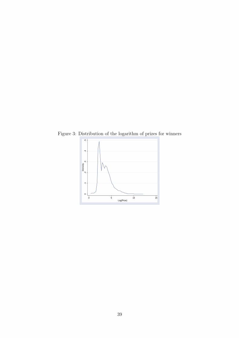
Figure 3: Distribution of the logarithm of prizes for winners

0.1

.2.3

.4.5

Density

0 5 10 15Log(Prize)

39

Figure 4: Non-Players, Players who do not win and Winners

Players

Winners

Non-Players

Observed

Not Observed

40