Wind Tunnel Study the Turbulence Effects on Aerodynamics of Suspended Truss Bridge

*Hoang Trong Lam 1), Hiroshi Katsuchi 2) and Hitoshi Yamada 3)

1), 2), 3) Dept. of Civil Engineering, Yokohama National University, Yokohama 240-8501, Japan

1) hoanglam289@gmail.com

ABSTRACT This paper presents the results from a state space system identification extraction flutter derivatives under difference turbulent flows. The aim of the study is to clarify the effects of oncoming turbulence on the flutter of suspended long span bridges deck by using section model wind tunnel test. Several wind tunnel tests on a trussed deck section have been carried out with different oncoming turbulent properties involve reduced turbulence intensities and turbulent scales. The analysis includes the investigation on: the effect of modal dynamic responses on oncoming flows. Next, the transient and buffeting responses data from wind tunnel test have been analysis by the system identification technique in extracting flutter derivatives (FDs) and the difficulties involved in this method are discussed. The time domain analysis stochastic system identification (DATA-SSI) is proposed to extract simultaneously all FDs from ones and two degree of freedom systems. Finally, the results under different conditions was discussed and concluded. 1. INTRODUCTION The wind in the atmospheric boundary layer is always turbulence. Any study of wind-induced vibration problems must confront this issue either by matching turbulence characteristics completely or by acknowledging uncertainty in conclusions as a result of imperfect simulations. Not many researches have focused clearly on the effects of turbulence on aeroelastic forces. Scanlan & Lin (1978) are the pioneers who used a trussed deck section model then concluded that flutter derivatives has an insignificant difference between smooth and turbulent flows. However, Huston conducted test on a model of the Golden Gate Bridge deck section and the results are different from that by Scanlan & Lin (1978) (Haan & Kareem 2007). Study on the effects of turbulent flows on flutter derivatives, the free vibration technique of sectional model used and application system identifications technique to extract FDs is widely. Various system identifications

1)

PhD Student 2),3)

Professor

technique was developed by many authors: the Extended Kalman Filter Algorithm (Yamada et al. 1992), Modified Ibrahim Time Domain (Sarka et al. 1994), Unifying least-squares method (Gu et al. 2000), Iterative least-squares method (Chowdhurry and Sarkar. 2003). In these systems the buffeting force and their response are considered as external noise, so this causes more difficulties at high wind velocity and especially, appears turbulence. Bartoli and Righi (2006) used CSIM (combined system identification method) is based on Sarkar MITD to extract simultaneously all FDs from a 2DOF rectangular section model. The conclusion is that identification of flutter derivatives in turbulent flow resulted satisfactory in spite of the difficulties encountered due to the process caused by the locally induced noise owing to signature of turbulence. The main reason is that, the CSIM is the deterministic system identification and the effects of turbulence are regarded as a more noisy-input signal to the system makes more problems in the identification process. Nikitas, Macdonal and Jakobsen (2011) are employed to extract FDs from ambient vibration data from full-scale monitoring using more elaborate stochastic identification technique (CBHM) (Jakobsen et al. 1995), and the study also illustrated the viability of system identification techniques for extracting valuable result from full-scale data. Boonyapinyo et al. (2010) applied data-driven stochastic subspace identification technique (SSI-DATA in short) to extract the FDs of bridge deck from wind tunnel test under both smooth and turbulent flows. The conclusion of this paper is that the SSI-DATA can be used to estimate FDs from buffeting responses with reliable results and an advantage of stochastic system is that it considers the buffeting force and response like input instead of noise. Therefore, the ratio of signal to noise is not affected by wind speed and the flutter derivatives at high wind speeds are readily available. Kirkegaard & Andersen (1997) compared three state spaces systems: stochastic subspace identification (SSI), stochastic realization estimator matrix block Hankel (MBH) and prediction error method (PEM). The results show that the SSI gives good results in terms of estimated modal parameters and mode shapes; the MBH is seen to give poor estimates of the damping ratios and the mode shapes compared with the other two techniques; and the SSI is approximately ten times faster than the PEM. In addition, there is a shortcoming involved in the free vibration technique; at high wind velocities the extraction FDs cannot be obtained accurately because the aerodynamic damping of vertical mode is too high and vertical free-vibration data is not long enough for analysis. From these considerations which bring the idea for applying the stochastic system identification (SSI) to estimate the FDs from gust responses of bridge trussed deck section. In this paper concentrates on the investigation of turbulent effects on FDs of bridge deck by employing a section model wind tunnel test in a turbulent flow. The output only system identification DATA-SSI is proposed to extract FDs from buffeting response. Tests are also carried out with the free vibration method in order to compare with proposed method.

2. EXPIREMENTAL SETUP AND TURBULENT GENERATION

A wind tunnel test was conducted in a closed-circuit wind tunnel at Yokohama National University. The working cross-section is 1.8m wide and 1.8m high. The

investigated profile is trussed deck section (Fig. 1). It was fabricated by wood with a scale 1:80 to represent the cross-section of long-span suspended bridge. The width and depth of the section-model are 363mm, and 162.5mm, respectively. The unit mass 8.095 kg/m and moment of inertia 0.2281 kg.m2/m. The section is attached to a rigid frame and at each corner supported by a linear spring with stiffness k. The mounting position of spring was adjusted for the elastic center and the gravity center of the cross section coincided. The cross-section was also to restrain motions in a desired degree of freedom while performing tests. The tests have been carried out in both smooth and different turbulence flows.

Fig. 1 Trussed deck sectional model The turbulent flows used in this study were generated with biplane wooden grid. The turbulent properties are controlled by changing the distances to the model. The flow conditions and turbulence properties are following:

(a) along wind turbulence (b) vertical wind turbulence

Fig. 2 Probability density function of longitudinal and vertical velocity fluctuation 2.1 Probability density function The probability density function of fluctuated wind speed is customarily with Gauss distribution. Fig. 2 shows both longitudinal and vertical wind speed fluctuation fairly good agreement with Gauss distribution.

2.2 Reduced turbulence intensity

Based on matching the power spectrum of turbulent flow in wind tunnel and full-scale spectral density function, H. Katsuchi and H. Yamada (2011) introduced reduced turbulence intensity which can be written as shown below:

3/1/ DL

II

x

u

ur (1)

where Iu – the turbulence intensity for the along-wind turbulence component is defined as: Iu u u is the standard deviation of the turbulence component and U is the

mean wind velocity; D is the height of cross-section model; x

uL is the integral length

scale for the turbulence component in the longitudinal direction. In this study the integral scale is defined as:

peak

x

un

UL

2

1 (2)

npeak is the frequency at which the curve reduced spectrum reaches a maximum. The length scale calculated from Eq. (2) is reasonable compared with the autocorrelation method, because the autocorrelation of turbulence component in several cases is just asymptotic to abscissa due to the area under autocorrelation curve and abscissa quite large. However, it was pointed in E. Simiu and H. Scanlan

(1996) that the estimation of x

uL based on measured value of U and npeak can be in

error several fold, owing to the sensitivity of x

uL to the assumption concerning the

spectral shape between n = 0 and n = npeak. Fig. 3 depicts the results of three

turbulence parameters Iu, Ir, and x

uL corresponding to different grid-to-model distances,

case 1 the distance around 4.8m, case 2 around 3.4m and case 3 around 2m with vary mean wind velocities. As in Fig. 3 shown that the average parameters case 1: Iu =

6.17%, Ir = 6.97% and x

uL = 11.26cm; case 2: Iu = 9.11%, Ir=11.09% and x

uL = 9.04cm;

case 3: Iu = 15.63%, Ir = 21.02% and x

uL = 6.79cm. The reduced turbulence intensities

increase the proportional with turbulence intensity but the inverse is true for integral length scale. Table 1 Turbulent flow parameters

Parameter Case 1 Case 2 Case 3

Iu (%) 6.17 9.11 15.63

Lux (cm) 11.26 9.04 6.79

Ir (%) 6.97 11.09 21.02

2.3 Turbulence power spectral density The turbulence intensity and integral length scale do not fully describe a properties of turbulent oncoming flows, because thanks to Y. Nakamura and S. Ozono (1987) studied on bluff-body aerodynamic shown that small-scale turbulence affects flow fields and aerodynamic paremeters more than larger one. Therefore the power spectral distribution of turbulence scales was also quantified for this research. Fig. 4a shows the non-dimensional frequency distribution of turbulent along-wind velocity component versus non-dimensional power spectral density function and matching between the power spectrum of simulated data from wind tunnel and empirical atmospheric turbulence von Karman and Eurocode 1. Compared with von Karman spectrum, the measured data coinccided well with it in the high frequency and it was a little higher in the low frequency. Turbulent energy is generated in larger eddies (low frequency). For most structure, these low-frequency fluctuations give no significant response contribution. In Fig. 4b, three spectra obtained at different reduced turbulent intensity (turbulent intensity) are shown. Values of the spectral density function increase as the reduced turbulence intensity is increased.

(a) (b)

Fig. 4 Power spectral density function for the longitudinal turbulence component

3. MODEL DYNAMIC RESPONSES

Tests have been conducted under both smooth and turbulence flows. The aim of this testing is to quantify the effect of oncoming turbulence flows on the dynamic responses of the section model. Fig. 5 illustrates the vibration amplitude of two degree of freedom (heaving and torsional mode) versus reduced wind velocities under smooth and different turbulence flows. Abbreviation of „RSM‟ is root-mean-square; „Max‟ is maximum amplitude of vibration; „Smooth‟ is smooth flow condition. In smooth flow, the vertical vibration is limited when reduced wind speed is from 0 to 9 and then considerably increases but vertical flutter does not occur in this test (Fig. 5a). On the

Non-dimensional frequency, fL=nLu/U

Non-d

ime

nsio

n P

SD

-nS

(n)/

u2

Frequency

(Hz)

PS

D-S

(n)

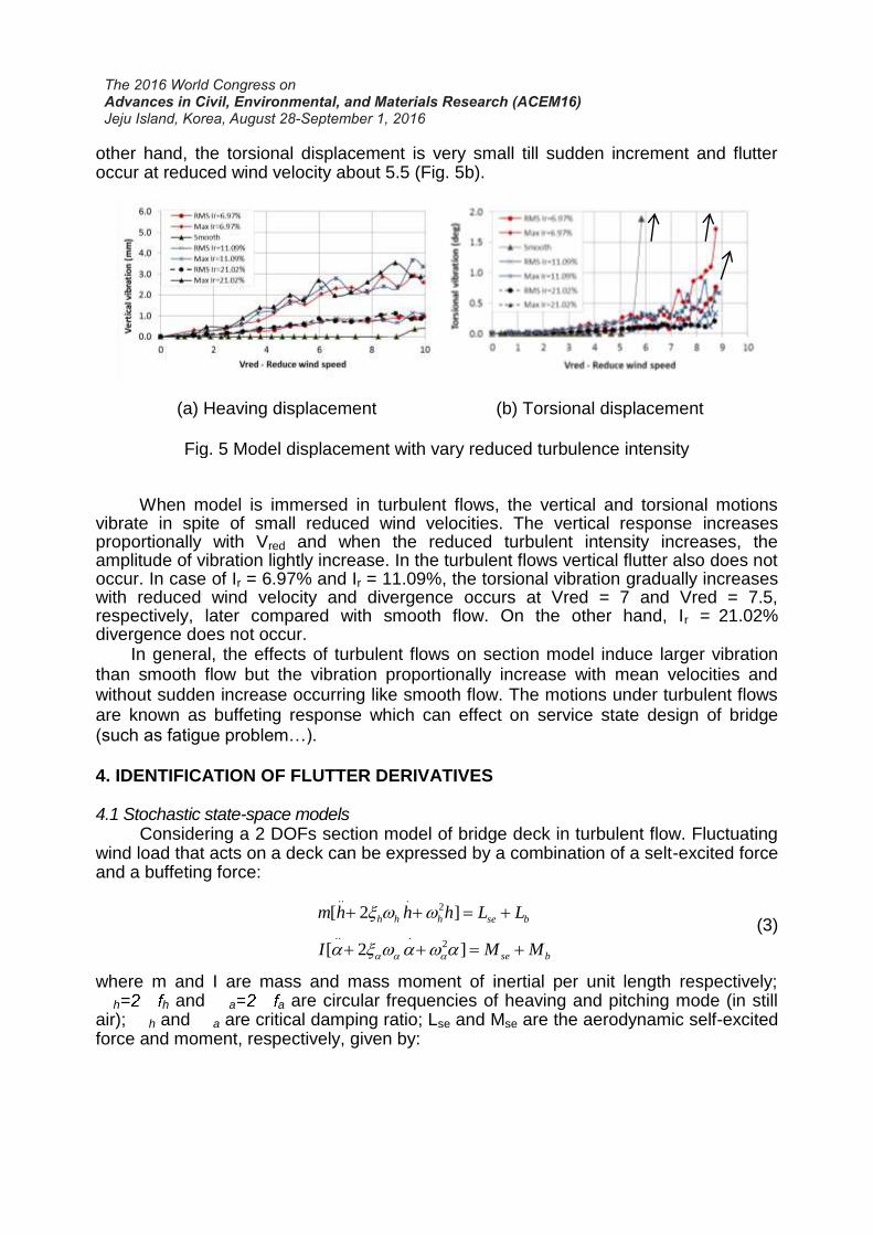
other hand, the torsional displacement is very small till sudden increment and flutter occur at reduced wind velocity about 5.5 (Fig. 5b).

(a) Heaving displacement (b) Torsional displacement

Fig. 5 Model displacement with vary reduced turbulence intensity

When model is immersed in turbulent flows, the vertical and torsional motions vibrate in spite of small reduced wind velocities. The vertical response increases proportionally with Vred and when the reduced turbulent intensity increases, the amplitude of vibration lightly increase. In the turbulent flows vertical flutter also does not occur. In case of Ir = 6.97% and Ir = 11.09%, the torsional vibration gradually increases with reduced wind velocity and divergence occurs at Vred = 7 and Vred = 7.5, respectively, later compared with smooth flow. On the other hand, Ir = 21.02% divergence does not occur. In general, the effects of turbulent flows on section model induce larger vibration than smooth flow but the vibration proportionally increase with mean velocities and without sudden increase occurring like smooth flow. The motions under turbulent flows are known as buffeting response which can effect on service state design of bridge (such as fatigue problem…). 4. IDENTIFICATION OF FLUTTER DERIVATIVES

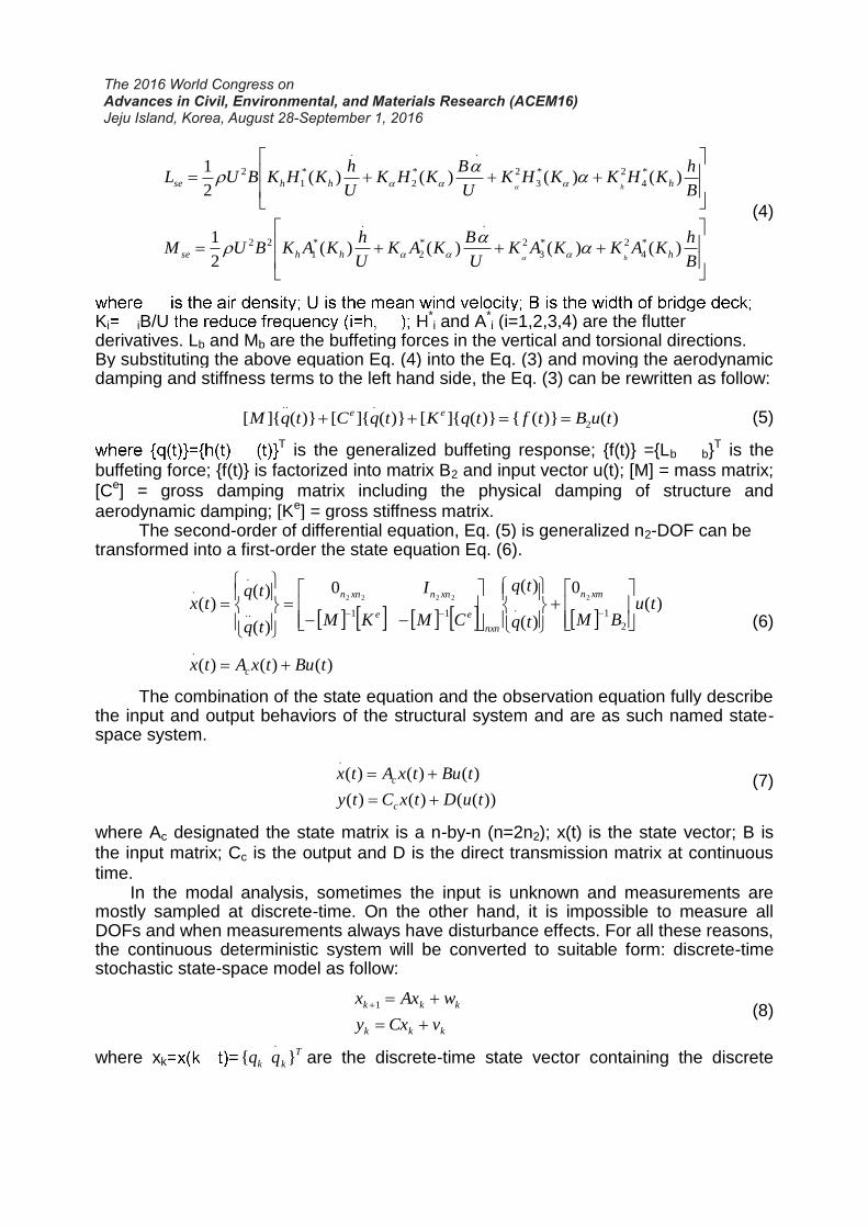
4.1 Stochastic state-space models Considering a 2 DOFs section model of bridge deck in turbulent flow. Fluctuating wind load that acts on a deck can be expressed by a combination of a selt-excited force and a buffeting force:

bse

bsehhh

MMI

LLhhhm

]2[

]2[

2...

2...

(3)

where m and I are mass and mass moment of inertial per unit length respectively;

h h and a a are circular frequencies of heaving and pitching mode (in still air); h and a are critical damping ratio; Lse and Mse are the aerodynamic self-excited force and moment, respectively, given by:

B

hKAKKAK

U

BKAK

U

hKAKBUM

B

hKHKKHK

U

BKHK

U

hKHKBUL

hhhse

hhhse

h

h

)()()()(2

1

)()()()(2

1

*

4

2*

3

2

.

*

2

.

*

1

22

*

4

2*

3

2

.

*

2

.

*

1

2

(4)

Ki iB/U *i and A*

i (i=1,2,3,4) are the flutter derivatives. Lb and Mb are the buffeting forces in the vertical and torsional directions. By substituting the above equation Eq. (4) into the Eq. (3) and moving the aerodynamic damping and stiffness terms to the left hand side, the Eq. (3) can be rewritten as follow:

)()}({)}(]{[)}(]{[)}(]{[ 2

...

tuBtftqKtqCtqM ee (5)

T is the generalized buffeting response; {f(t)} ={Lb b}T is the

buffeting force; {f(t)} is factorized into matrix B2 and input vector u(t); [M] = mass matrix; [Ce] = gross damping matrix including the physical damping of structure and aerodynamic damping; [Ke] = gross stiffness matrix. The second-order of differential equation, Eq. (5) is generalized n2-DOF can be transformed into a first-order the state equation Eq. (6).

)()()(

)(0

)(

)(0

)(

)()(

.

2

1.

11..

.

.22222

tButxAtx

tuBMtq

tq

CMKM

I

tq

tqtx

c

xmn

nxn

ee

xnnxnn

(6)

The combination of the state equation and the observation equation fully describe the input and output behaviors of the structural system and are as such named state-space system.

))(()()(

)()()(.

tuDtxCty

tButxAtx

c

c

(7)

where Ac designated the state matrix is a n-by-n (n=2n2); x(t) is the state vector; B is the input matrix; Cc is the output and D is the direct transmission matrix at continuous time. In the modal analysis, sometimes the input is unknown and measurements are mostly sampled at discrete-time. On the other hand, it is impossible to measure all DOFs and when measurements always have disturbance effects. For all these reasons, the continuous deterministic system will be converted to suitable form: discrete-time stochastic state-space model as follow:

kkk

kkk

vCxy

wAxx

1 (8)

where xkT

kk qq }{.

are the discrete-time state vector containing the discrete

sample displacement qk and velocity kq.

; wk is the process noise due to disturbances and modelling inaccuracies; vk is the measurement noise due to sensor inaccuracy. Following assumption wk and vk is zero mean and with covariance matrix:

pqT

T

q

T

q

p

p

RS

SQvw

v

wE

(9)

where the index p and q are time- pq is the Kronecker delta. As the correlation E(wp wq

T) and E(vp vqT) are equal zero in case of

different time-instant. Further the stochastic model is assumed that {xk}, {wk} and {vk} are mutual independent: E(xk wk

T)=0 and E(xk vkT)=0. According to Peeters & Roeck

(1999) proven that the output covariance R=E[yk+i ykT] for any arbitrary time-

can be considered as impulse response (Eq. 10) of the deterministic linear time-invariance system A, C, G; where G= E[xk+1 yk

T] is the next state-output covariance matrix.

GCAR i

i

1 (10)

The classification of SSI based on the key step of these methods; by following Peeters & Roeck (1999), they are covariance-driven stochastic subspace identification (COV-SSI) and data-driven stochastic subspace identification (DATA-SSI). In this study the DATA-SSI used to extract FDs. 4.2 DATA-SSI

DATA-SSI works directly with time-series of experimental data, without need to convert out-put data to correlation, covariance or spectra. The main step of DATA-SSI is a projection of the row space of the future outputs into the row of past outputs. The orthogonal projection Pi is defined as:

p

T

pppfpfi YYYYYYYP 1)(/ (11)

Where the matrix Yf and Yp are the under half part and upper part half of a bock Hankel matrix H, defined as:

li

li

Y

Y

Y

Y

Y

Hf

p

ji

ij

ij

):2(

)12:2(

)2:1(

... (12)

where 2i are the number of block rows, j are the number of data points, l are the number of output sensors. The main theorem of stochastic subspace identification states that the projection Pi can be factorized as the product of observability matrix Oi

and the Kalman filter state sequence ^

iX (Peeters & Roeck 1999):

^

1

^

1

^^

1

...... iijii

i

i XOxxx

CA

CA

C

P

(13)

The observability matrix Oi and the Kalman filter sequence ^

iX are obtained by applying

SVD to the projection matrix:

T

i VSUP 111 (14)

Combining Eq. (13) and Eq. (14) gives:

iii POXSUO ^

2/1

11 , (15)

If the shifted past and future outputs of Hankal matrix another project is obtained:

1

^

11 /

iifi XOYYPp

(16)

Oi-1 is obtained from Oi after deleting the last l rows and the shifted state sequence can be computed in Eq. (16) as:

11

^

1

ii POX i (17)

From Eq. (15) and Eq. (17), the Kalman state sequences 1

^^

,ii XX are calculated using

only output data. The system matrices can now be recovered from over determined set of linear equations, obtained by extending Eq. (8):

v

w

i

ii

i XC

A

Y

X

^

/

1

^

(18)

where Yi/i is a Hankel matrix with only one block row. Since the Kalman state sequence

Tw T

v)T are uncorrelated with

^

iX , the

set of equation can be solved for A,C in a least-squares:

^

/

1

^

XY

X

C

A

ii

i (19)

4.3 Identification of flutter derivatives The modal parameters of system can be obtained by solving the eigenvalue problem state matrix A (Eq. 19):

CA ;1 (20)

the mode shape matrix. When the complex modal parameters known, the gross damping Ce and gross stiffness Ke in Eq. (5) is determined by following:

1

**

*

2**2 )(

MCK ee (21)

Let 0101

11

;

;

KMKCMC

KMKCMC eeee

where C0 and K0 the mechanical damping and stiffness matrix of system under no-wind condition. Thus, the flutter derivatives of two DOF can be defined as:

)(2

)(,)(2

)(

)(2

)(,)(2

)(

)(2

)(,)(2

)(

)(2

)(,)(2

)(

212124

*

4111123

*

4

222224

*

3121223

*

3

22224

*

212123

*

2

21213

*

111112

*

1

KKB

IkAKK

B

mkH

KKB

IkAKK

B

mkH

CCB

IkACC

B

mkH

CCB

IkACC

B

mkH

e

h

h

e

h

h

e

h

e

ee

e

h

h

e

h

h

(22)

5. FLUTTER DERIVATIVES AND COMPARISON

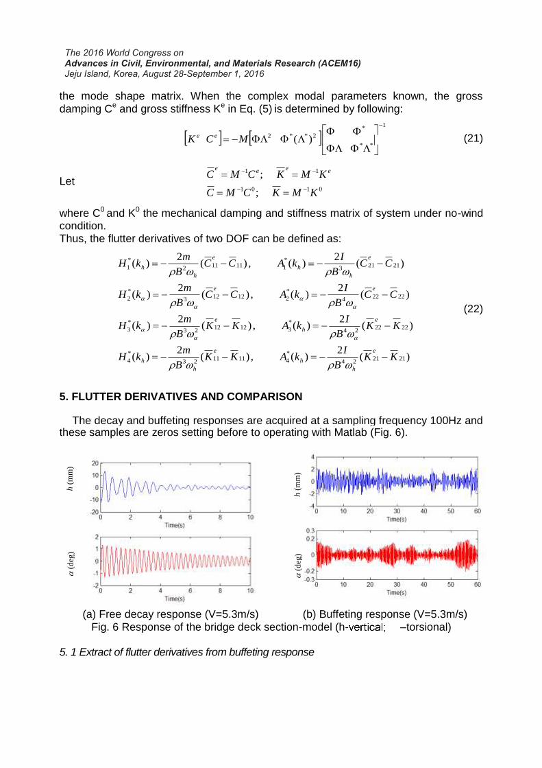
The decay and buffeting responses are acquired at a sampling frequency 100Hz and

these samples are zeros setting before to operating with Matlab (Fig. 6).

(a) Free decay response (V=5.3m/s) (b) Buffeting response (V=5.3m/s) Fig. 6 Response of the bridge deck section-model (h- –torsional)

5. 1 Extract of flutter derivatives from buffeting response

h (

mm

)

(d

eg)

h (

mm

)

(d

eg)

At high wind velocity, the aerodynamic damping of heaving mode is too high and vertical

Fig. 7 FDs (Hi) of the bridge section-model by SDOF test and coupled test by

free decay and buffeting responses (case Ir=11.09%)

Fig. 8 FDs (Ai) of the bridge section-model by SDOF test and coupled test by

free decay and buffeting responses (case Ir=11.09%)

free response is too short; therefore, the extraction of FDs cannot be accomplished high accuracy. The bridge deck section-model will vibrate under the excitation of turbulent flows even at small wind velocity, it is reasonable to extract FDs from buffeting response. Fig. 7&8 show the flutter derivatives of bridge deck by the DATA- SSI method from both free decay and buffeting responses of 1DOF and 2DOF systems under turbulence flows (Ir=11.09%). Overall, most FDs are in good agreement with both free decay and buffeting response of 1DOF and 2DOF systems, except FDs related to vertical frequency and vertical damping (H1

* and H4*). The difference may be

explained by short data to recode under free decay test. The coupled aerodynamic derivatives (H2

* and H3*) extracted from buffeting responses are more scattering than

from free decay, especially at high reduced wind speed. At small wind velocity, the amplitude of buffeting vibration is small and the high damping torsional mode is not fully excited, so the FDs is less accurate (A2

*).

5. 2 The effects of turbulence on flutter derivatives

Fig. 10 & 11 illustrate the flutter derivatives of heaving and torsional mode under smooth and turbulent flows with the difference reduced turbulence intensity. In these derivatives, the torsional damping term A2

*; plays an important role on torsinal flutter stability, since its positive/negative value corresponds to the aerodynamic instability/stability of torsinal fluter. On the other hand, the coupled term, H3

* and A1*,

and the aerodynamically un-coupled derivative A2* have significant role on heaving-

torsional of 2DOF coupled flutter instability (Matsumoto 2001). As shown in Fig. 9 & 11, under smooth flow, the positive value A2

* at high reduced wind speed (Vred>5.5) and total torsional damping are almost controled by A2

*, the coupling

a. Damping ratio of heaving mode b. Damping ratio of torsional mode Fig. 9 Damping ratio of the bridge section-model under smooth and turbulence

flows

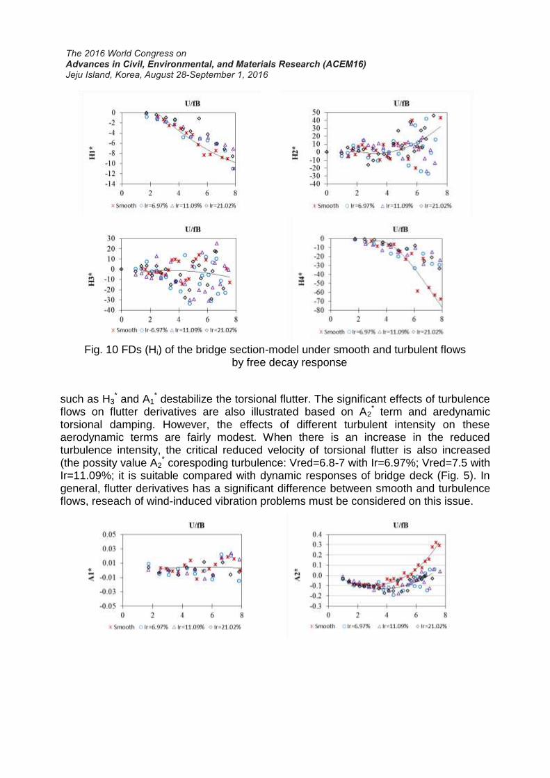
Fig. 10 FDs (Hi) of the bridge section-model under smooth and turbulent flows

by free decay response

such as H3* and A1

* destabilize the torsional flutter. The significant effects of turbulence flows on flutter derivatives are also illustrated based on A2

* term and aredynamic torsional damping. However, the effects of different turbulent intensity on these aerodynamic terms are fairly modest. When there is an increase in the reduced turbulence intensity, the critical reduced velocity of torsional flutter is also increased (the possity value A2

* corespoding turbulence: Vred=6.8-7 with Ir=6.97%; Vred=7.5 with Ir=11.09%; it is suitable compared with dynamic responses of bridge deck (Fig. 5). In general, flutter derivatives has a significant difference between smooth and turbulence flows, reseach of wind-induced vibration problems must be considered on this issue.

Fig. 11 FDs (Ai) of the bridge section-model under smooth and turbulent flows

by free decay response 6. CONCLUSIONS This study investigated the effects of turbulence on flutter derivatives of trussed bridge deck section by using wind-tunnel test and out-put only state space stochastic system identification technique identified flutter derivatives from vary DOF and excitation. Conclusions from this study are summarized here: DATA-SSI methods show a good result even under turbulence flows because an advantage of those methods is considered buffeting force and response as inputs instead of noises. An identification of flutter derivatives from buffeting responses is plausible, the advantage of this technique is easier to obtain buffeting response, and the section-model will be oscillated under wind flow, moreover, in turbulence flows. This is less time consuming than free decay test. Especially at high wind velocity the vertical free decay data is too short, it is causes less accuracy. Turbulence flows significantly affect on dynamic responses and flutter derivatives of trussed bridge deck section, specifically, turbulence induces larger displacement but incease critical divergence velocity are also illustrated based on buffeting response and aredynamic torsional damping term A2

*. Using the proposed framework, the variety of aerodynamic features were addressed, which helped us better understand the effect of different flows on aerodynamics of trussed bridge deck section. REFERENCES Bart Peeters and Guido De Roeck (1999), “Reference-based stochastic subspace

identification for output-only modal analysis”, Mechanical Systems and Signal Processing, 13(6), 855-878.

Bartoli, G., Contri, S., Mannini, C. and Righi, M. (2009), “Toward an improvement in the identification of bridge deck flutter derivatives”, J. of Eng. Mech. ASCE, Vol. 135, 771-785.

Bartoli, G., Righi, M. (2006), “Flutter mechanism for rectangular prism in smooth and turbulent flow”, J. Wind Eng. Ind. Aerodyn, Vol. 94, 275-291.

Boonyapinyo, V., Janesupasaeree, T. (2010), “Data-driven stochastic subspace identification of flutter derivatives of bridge decks”, J. Wind Eng. Ind. Aerodyn, Vol. 98, 784-799.

Chowdhury, A.G., Sarkar, P.P. (2003), “A new technique for identification of eighteen flutter derivatives using three-degrees-of-freedom section model”, Engineering Structures, Vol. 25, 1763-1772.

Claes Dyrbye and Svend O. Hansen (1997), “Wind Loads on Structures”, John Wiley & Sons, New York.

Haan, F.L. (2000), “The effects of turbulence on the aerodynamics of long-span bridges”, Ph.D. Dissertation; University of Notre Dame, US.

Haan, F.L., Kareem, A. (2007), “The effects of turbulence on the aerodynamics of oscillating Prisms”, ICWE12 CAIRNS, 1815-1822.

Yamada, H., Miyata, T. and Ichikawa, H. (1992), “Measurement of aerodynamic coefficients by system identification method”, J. Wind Eng. Ind. Aerodyn, Vol. 42, 1255-1263.

Katsuchi, H. and Yamada, H. (2011), “Study on turbulence partial simulation for wind-tunnel testing of bridge deck”, Proc. of ICWE 13, Amsterdam, Netherlands.

Kirkegaar, P.H. and Andersen, P. (1997), “State space identification of civil engineering structures from output measurement”, Proc. of the 15th International Modal Analysis Conference, Orlando, Florida, USA.

Matsumoto, M., Tamwaki, Y. and Shijo, R. (2001), “Frequency characteristics in various flutter instabilities of bridge girders”, J. Wind Eng. Ind. Aerodyn, Vol. 89, 385-408.

Nikitas, N., Macdonal, J.H.G. and Jakobsen, J.B. (2011), “Identification of flutter derivatives from full-scale ambient vibration measurements of the Clifton suspension bridge”, J. Wind and Struct., Vol. 14, 221-238.

Nakamura, Y. and Ozono, S. (1987), “The effects of turbulence on a separated and reattaching flow”, J. Fluid Mech., Vol. 178, 477-490.

Scanlan, R.H. and Lin, W.H. (1978), “Effects of turbulence on bridge flutter derivatives”, J. Eng. Mech. Div., Vol.104, 719-733.

Scanlan, R.H. (1997), “Amplitude and turbulence effects on bridge flutter derivatives”, J. Struct. Eng. ASCE, Vol. 123, 232-236.

Simiu, E. and Scanlan, R.H. (1996), “Wind Effects on Structures”, 3rd edition, John Wiley & Sons, New York.

Sarkar, P.P., Jones, N.P, Scanlan, R.H (1992), “System identification for estimation of flutter derivatives”, J. Wind Eng. Ind. Aerodyn, Vol. 42, 1243-1254.

Peeters B., and Roeck, G.D. (1999), Reference based stochastic subspace identification for output-only modal analysis”, Mech. Systems and Signal Processing, (13(6)), 855-878.

Juang, J.N., and Pappa, R.S. (1985), “An eigensystem realization algorithm (ERA) for modal parameter identification and model reduction”, J. Guid. Contr. Dyn., 299-318.

Jakobsen, J.B, Hjorth-Hansen, E. (1995), “Determination of the aerodynamic derivatives by a system identification method”, J. Wind Eng. Ind. Aerodyn, Vol. 57, 295-305.