WILSONVILLE HIGH SCHOOL

8

Analysis of Designed Experiments

8.1 Introduction

In this chapter we discuss experiments whose main aim is to study andcompare the effects of treatments (diets, varieties, doses) by measuringresponse (yield, weight gain) on plots or units (points, subjects, patients).In general the units are often grouped into blocks (groups, sets, strata) of‘similar’ plots or units.

We assume we have a response y which is continuous (for example,a normal random variable). We also have possible explanatory variableswhich are discrete or qualitative, called factors. Here we consider treat-ment factors whose values are assigned by the experimenter. The valuesor categories of a factor are called levels, so that the levels of a treatmentfactor are labels for the different treatments. For example, in comparingengineering components from several different manufacturers, we could de-fine indicator variables to denote the manufacturer. If there are k differentmanufacturers, one way to do it is to define

xij ={

1 if component i comes from manufacturer j,0 otherwise, (8.1)

for j = 1, 2, ..., k − 1. We do not need to define xik because if xi1 = ... =xi(k−1) = 0 then it automatically follows that component i is from manu-facturer k. It is possible to use the regressor variables defined by 8.1, eitheron their own or in conjunction with other continuous regressors, to fit alinear regression model using standard software. If that were all there wasto it, we would not need a separate theory for the analysis of variance.However, the specific issues raised by these models are such as to justifyand require a detailed treatment in their own right.

8.2 Completely Randomized Design

We allocate r treatments randomly to the n sample units such that the ithtreatment is allocated to ni units (i = 1, 2, . . . , r) (i.e. each treatment hasni replications). Note there is no blocking here: very often in experimental

Chapter 8. Analysis of Designed Experiments 389

design, the units are blocked into groups of similar units before being allo-cated to treatments, but we are not assuming that kind of experiment yet(see Section 7.3) — all n =

∑i ni units are regarded as ‘similar’ and there

is one treatment factor with r levels. If the ni are all equal, then the exper-iment is called balanced. Note that a completely randomized design withr = 2 gives an experiment which is the same set-up as for a two-sample t-test (Appendix A). An experiment with two treatments arranged in blocks,so that each block contains one member assigned to the first treatment andone member assigned to the second, corresponds to a matched pairs t-test.

For the completely randomized design we use the one-way model

yij = µ + αi + εij

where j = 1, 2, . . . , ni, i = 1, 2, . . . , r and∑r

i=1 ni = n. In this model yij

is the response of the jth unit receiving the ith treatment, µ is an overallmean effect, αi is the effect due to the ith treatment and εij is randomerror. Another natural way to write this model is

yij = µi + εij

where j = 1, 2, . . . , ni, i = 1, 2, . . . , r and∑r

i=1 ni = n. The only differencebetween these two models is that µi is used to denote the total response totreatment i. The first specification has the advantage that αi has a specificinterpretation as a “treatment effect” associated with treatment i.

We have the usual least squares assumptions that the εijs have zeromean and constant variance σ2 and are uncorrelated. In addition we usu-ally make the normality assumption that the εijs are independent normalrandom variables. Together these mean that

yij ∼ N(µ + αi, σ2)

and are independent.We may note the following:

1. If treatment acts multiplicatively on the response, where yij = µαiεij

(where in this kind of model εij > 0 for all i and j), then the varianceof yij is non-constant, but by taking logarithms of the response, theone way model may then be valid. (The model assumes the varianceis the same for each treatment group.)

2. Units, even in the same treatment group, are assumed to be uncorre-lated.

3. The original response may need to be transformed to achieve normality.Within this framework, some of the questions that we might want to

answer include(a) estimating the µis, or equivalently µ and the individual αis,

390 Chapter 8. Analysis of Designed Experiments

(b) estimating linear combinations of the µis or αis, especially contrasts:linear combinations of the form

∑i ciαi where

∑i ci = 0,

(c) testing equality of all the µis, or equivalently the hypothesis H0 : α1 =... = αr = 0.

Theoretical treatments of the analysis of variance often focus undulyon objective (c), though it is important to remember that this is rarely aninteresting objective in its own right. It may well be a necessary preliminaryto some more meaningful question such as determining which of severaldrugs or agricultural varieties is the best, or whether any of a numberof engineering manufacturers is differing unacceptably from a predefinedstandard.

We can write the model in matrix form y = Xβ + ε,

y11

y12...

y1n1

y21

y22...

yrnr

=

1 1 0 0 . . . 01 1 0 0 . . . 0...

......

.... . .

...1 1 0 0 . . . 01 0 1 0 . . . 01 0 1 0 . . . 0...

......

.... . .

...1 0 0 0 . . . 1

µα1

α2...

αr

+

ε11ε12...

ε1n1

ε21ε22...

εrnr

.

We can estimate the unknown parameters β = (µ, α1, α2, . . . , αr) byleast squares or equivalently by maximum likelihood under the normalityassumption by solving the normal equations

(XT X)β = XT y.

These are (r + 1) equations in (r + 1) unknowns. We have

XT X =

n n1 n2 . . . nr

n1 n1 0 . . . 0n2 0 n2 . . . 0...

......

. . ....

nr 0 0 . . . nr

,

XT y =

∑i

∑j yij∑

j y1j∑j y2j

...∑j yrj

=

GT1

T2...

Tr

,

where G is the grand total and Ti is the total for the ith treatment.


The normal equations are therefore

nµ +r∑

i=1

niαi =∑

i

∑

j

yij , (8.2)

niµ + niαi =∑

j

yij i = 1, 2, . . . , r. (8.3)

The equations are not independent as the sum over i in (8.3) equals thetotal in (8.2), so there are only r equations for r + 1 unknowns and thereare infinitely many solutions. However, this does not prevent the modelbeing estimated, because the fitted values are always the same whicheversolution is chosen and hence the residuals and residual sum of squares arethe same.

In order to solve the equations we have to add another equation orconstraint on the estimates. Consider three possible constraints:

1. Applying the constraint∑

i niαi = 0 imples that µ equals the overallmean,

µ = y =G

n=

∑∑yij

n.

Hence αi is estimated by

αi = yi· − y··

where yi· =∑

j yij/ni and y·· =∑

i

∑j yij/n.

2. A second method is to set µ = 0, so that

αi = Ti/ni = yi·

3. Take α1 = 0. This is the solution adopted by some statistical packagese.g. GLIM. It follows that µ = y1. and hence that

αi = yi· − y1. for i = 2, 3, . . . , n.

For each of the three solutions the fitted values (estimated means) are

µ + αi = yi·

for a unit in the ith treatment group. So the fitted values are identical, asare the residuals,

eij = yij − yi·,

the residual sum of squares (SSE or deviance) and hence s2. The residualsum of squares is given by

SSE =∑

i

∑

j

(yij − yi·)2.


8.2.1 The ANOVA Table

As in Chapters 2 and 3, a convenient way to represent the results of an anal-ysis of variance is through a table known as the ANOVA table. Althoughthis is mathematically just a special case of the general development inSection 3.5, it is useful to re-derive the results directly for this model.

The total (corrected) sum of squares is

SSTO =∑

i

∑

j

(yij − y··)2,

which is also known as the deviance after fitting the null model yij = µ+εij ,i.e. a model with no treatment effects, α1 = α2 = . . . = αr = 0. The totalsum of squares SSTO can be decomposed:

∑

i

∑

j

(yij − y··)2

=∑

i

∑

j

[(yij − yi·) + (yi· − y··)]2

=∑

i

∑

j

(yij − yi·)2 +∑

i

ni(yi· − y··)2 + 2∑

i

(yi· − y··)∑

j

(yij − yi·)

=∑

i

∑

j

(yij − yi·)2 +∑

i

ni(yi· − y··)2

sinceni∑

j=1

(yij − yi·) = 0.

HenceSSTO = SSE + SSTR

where SSE is the deviance under the full model

yij = µ + αi + εij .

The SSTR is the “sum of squares due to treatments”, analogous to SSRin an ANOVA table for regression. It is the difference in deviances betweenthe null model and the full model, in other words, the extra sum of squaresdue to the treatment effects or the increase in deviance when we assumeH0 : α1 = · · · = αr = 0 to be true. This is the extra sum of squares dueto H0. In order to test H0, note that

E{SSE} = E{∑

i

∑

j

(yij − yi·)2}


=∑

i

E{∑

j

(yij − yi·)2}

=∑

i

(ni − 1)σ2

= (n− r)σ2

and hence

s2 =SSE

n− r

is an unbiased estimate of σ2. Note that the divisor is total number ofobservations minus number of independent parameters, which is also thetotal number of degrees of freedom when the treatment means are uncon-strained. Under the null model yij = µ + εij , all treatments have the sameeffect. If H0 is true

E{SSTO} = (n− 1)σ2

and

E{extra SS due to treatments} = (n− 1)σ2 − (n− r)σ2

= (r − 1)σ2

Hence if H0 is trueSSTR

r − 1

is an unbiased estimate of σ2. Under the normality assumption it can beshown that

SSTR

σ2∼ χ2

r−1

andSSE

σ2∼ χ2

n−r

and that they are independent. Hence

F =SSTR/(r − 1)SSE/(n− r)

=Treatment Mean Square

s2∼ Fr−1,n−r (8.4)

under H0. So we reject H0 (and hence conclude that there are significantdifferences among the treatments) if F > Fr−1,n−r;1−α.

The whole information may be summarized in the form of an analysisof variance (ANOVA) table as in Table 8.1.


Source DF SS MS F

Treatments r − 1∑

iT 2

i

ni− G2

nSSr−1

SS/(r−1)s2

Residual n− r by subtraction s2

Total n− 1 SSTO =∑

i

∑j y2

ij − G2

n

Table 8.1 ANOVA table for one-way analysis of variance.

8.2.2 Testing equality of variancesThe preceding analysis has assumed that the variances are the same in allsamples. If the variances are allowed to be completely arbitrary, then thereis no exact procedure to test equality of the means — in the case r = 2,this is just the Behrens-Fisher problem discussed in Appendix A. However,it is advisable to test for the equality of variances. We describe here howto construct a likelihood ratio test for this.

Define Si =∑

j(yij − yi.)2 for i = 1, ..., r. Assume that yij ∼ N(µi, σ2i )

independently for all i and j, and consider testing H0 : σ21 = ... = σ2

r

against the alternative H1 that imposes no constraints on the {σ2i }. The

likelihood L, maximized with respect to {µi}, is given by

L ∝r∏

i=1

{(1σ2

i

)ni/2

exp(− Si

2σ2i

)}.

This is maximized with respect to σ2i by setting σ2

i = Si/ni. Hence themaximized likelihood under H1 is given, up to a constant of proportionality,by

L1 =r∏

i=1

{(1σ2

i

)ni/2

e−ni/2

}.

Under H0, we replace σ2i by a common σ2 in L, and maximize with respect

to σ2. This leads to σ2 =∑

i Si/N , and the resulting likelihood given by

L0 =(

1σ2

)N/2

e−N/2.

Consequently the log likelihood ratio statistic is

T = 2 log(

L1

L0

)=

r∑

i=1

ni log(

σ2

σ2i

). (8.5)

Under H0, the approximate distribution of this statistic is

T ∼ χ2r−1.


8.2.3 Bartlett’s modification

Bartlett (1937), in the earliest example of what is now known as the Bartlettcorrection, proposed a modification of this test to improve the χ2 approxi-mation.

The steps in this modification are:

1. Replace ni by ni − 1 everywhere, so that σ2i = Si/(ni − 1),

σ2 =∑

i Si/(N − r) and replace ni by ni − 1 in (8.5),2. With the definition of T thus modified, the distributional approxima-

tion is

{1 +

13(r − 1)

r∑

i=1

(1

ni − 1− 1

N − r

)}−1

T ∼ χ2r−1.

Hence reject H0 at level α if T > χ2r−1;1−α, the upper-α quantile of

the χ2r−1 distribution.

8.2.4 Two examples.

(i) The PEMA data.

Our first example is based on Streete et al. (1986).Table 8.2 gives the serum levels of 2-ethyl-2-phenylmalonamide (PEMA)

in patients receiving anticonvulsant medication. The aim is to measurePEMA levels in patients who are prescribed primidone either singly orin combination with other anticonvulsants. In this example we shall onlyconsider patients who had similar dose levels of each of the four drug com-binations listed below. The first group were given primidone alone, thesecond primidone and phenobarbitone, the third primidone and phenytoinand the last a combination of all three, primidone, phenobarbitone andphenytoin. We shall fit a one-way model and look for evidence to indicatereal differences among the four different drug combinations.

DRUG1 2 3 4

9.9 8.8 4.9 11.08.6 11.8 6.7 8.36.0 6.6 5.6 12.61.2 26.6 7.2 7.84.2 27.0 10.1 5.910.5 13.4 11.1 8.84.1 37.2 2.8 8.6

Table 8.2 PEMA data.


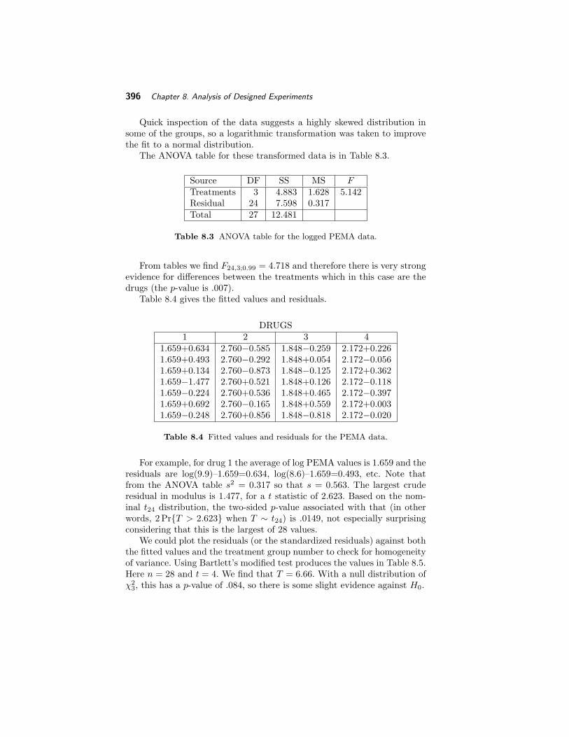
Quick inspection of the data suggests a highly skewed distribution insome of the groups, so a logarithmic transformation was taken to improvethe fit to a normal distribution.

The ANOVA table for these transformed data is in Table 8.3.

Source DF SS MS FTreatments 3 4.883 1.628 5.142Residual 24 7.598 0.317Total 27 12.481

Table 8.3 ANOVA table for the logged PEMA data.

From tables we find F24,3;0.99 = 4.718 and therefore there is very strongevidence for differences between the treatments which in this case are thedrugs (the p-value is .007).

Table 8.4 gives the fitted values and residuals.

DRUGS1 2 3 4

1.659+0.634 2.760−0.585 1.848−0.259 2.172+0.2261.659+0.493 2.760−0.292 1.848+0.054 2.172−0.0561.659+0.134 2.760−0.873 1.848−0.125 2.172+0.3621.659−1.477 2.760+0.521 1.848+0.126 2.172−0.1181.659−0.224 2.760+0.536 1.848+0.465 2.172−0.3971.659+0.692 2.760−0.165 1.848+0.559 2.172+0.0031.659−0.248 2.760+0.856 1.848−0.818 2.172−0.020

Table 8.4 Fitted values and residuals for the PEMA data.

For example, for drug 1 the average of log PEMA values is 1.659 and theresiduals are log(9.9)–1.659=0.634, log(8.6)–1.659=0.493, etc. Note thatfrom the ANOVA table s2 = 0.317 so that s = 0.563. The largest cruderesidual in modulus is 1.477, for a t statistic of 2.623. Based on the nom-inal t24 distribution, the two-sided p-value associated with that (in otherwords, 2Pr{T > 2.623} when T ∼ t24) is .0149, not especially surprisingconsidering that this is the largest of 28 values.

We could plot the residuals (or the standardized residuals) against boththe fitted values and the treatment group number to check for homogeneityof variance. Using Bartlett’s modified test produces the values in Table 8.5.Here n = 28 and t = 4. We find that T = 6.66. With a null distribution ofχ2

3, this has a p-value of .084, so there is some slight evidence against H0.


yi· 1.659 2.760 1.848 2.172s2

i 0.572 0.418 0.217 0.059ni 7 7 7 7

Table 8.5 Bartlett’s test for the PEMA data

(ii) Round-robin data.

Round-robin tests are tests performed under supposedly the same con-ditions in a series of laboratories. They play an important part in the stan-dardization of measurement procedures in physics and engineering. How-ever, the tests are often expensive to perform, so the results of such studiesare often small unbalanced sets of data.

Table 8.6 is based on an actual example of such a study into the mea-surement of the rate of creep rupture. Samples of a material were sent to 11laboratories which were asked to perform repeat measurements. Tabulatedare ni, the number of tests performed at laboratory i, and the mean andstandard deviation (S.D.) of the measurements made at laboratory i. Alsocomputed in column 5 is Si = (ni − 1)(S.D.)2. The last two columns willbe explained a little further on.

Laboratory i ni Mean S.D. Si αi S.E.1 5 102.1 48.1 9254.442 9 92.8 8.3 551.12 3.62 2.063 4 97.2 8.6 221.88 8.02 3.284 5 79.9 9.2 338.56 −9.28 2.905 5 87.0 4.8 92.16 −2.18 2.906 5 93.1 5.5 121.00 3.92 2.907 5 82.2 4.4 77.44 −6.98 2.908 6 54.9 1.9 18.059 5 94.0 8.3 275.56 4.82 2.90

10 5 90.4 2.2 19.36 1.22 2.9011 5 84.7 5.7 129.96 −4.48 2.90

Table 8.6 Round-robin test data

It can be seen immediately that the S.D. for laboratory 1 is much largerthan the others, and an application of (8.5) immediately confirms thatthis is significant: the likelihood ratio statistic is 103.3 with a nominal χ2

10

distribution. The 0.0001% point of χ210 is 46.9. In fact, the raw data for

laboratory 1 showed one extreme outlier which was not deleted from the


reported data, almost certainly due to a recording error. If we ignore theapparent discrepancy in variances and compute the F statistics (8.4) forequality of means, the F value is 3.86, which is highly significant (with anominal distribution of F10,48, the p-value is .0007). However, in this casethe discrepancy in variances is to some extent masking differences in themeans, and to avoid such a bias in other comparisons, we delete laboratory1 for the rest of the discussion.

To proceed with the analysis, deleting laboratory 1 and repeating thetests for the other 10 laboratories, (8.5) yields the test statistic 22.6, nom-inally χ2

9, which is still high (significant at 1% — actual p-value 0.007)but not nearly as bad as before. In this case, the F statistic in (8.4) is20.2, very highly significant against the nominal F9,44 distribution (theo-retical p-value about 10−13). Further inspection of the data indicates thatlaboratory 8 has a much lower mean than the others, and also the low-est standard deviation. Omission of laboratory 8 (as well as laboratory 1)leads to the test statistics 13.2 in (8.5), 3.67 in (8.4). The value 13.2 is notsignificant against χ2

8 at the 10% level, so seems acceptable for the equalityof variances.

If the likelihood ratio statistics (8.5) are modified by the Bartlett correc-tion, they become 77.9 for the full model with all 11 laboratories, 16.9 forthe model with laboratory 1 omitted, and 11.4 for the model with laborato-ries 1 and 8 both omitted. The modification in the first case is substantialbut irrelevant. The value 16.9 is almost exactly at the 5% point for χ2

9, sothe effect of the modification here is to conclude that the assumption ofequality of variances might just be acceptable in this case (with labora-tory 1 omitted), though since it is clear that laboratory 8 is discrepant inits mean value, this does not affect our overall conclusions. The correctionfrom 13.2 to 11.4 in the third model strengthens the conclusion that thevariances can be assumed equal in this case. Thus the Bartlett correctiondoes not change any of our conclusions, but it does turn out to be numeri-cally not negligible. In general it can be recommended that, in experimentsof this nature when the individual ni are small, it is worthwhile to applythe Bartlett correction.

For the final model, with laboratories 1 and 8 both omitted, an ANOVAtable is shown in Table 8.7. The final F statistic for the hypothesis of notreatment effect is 3.66, for a p-value of .003. Thus, we conclude that evenwhen laboratories 1 and 8 are omitted, there is still a significant differenceamong the remaining 9 laboratories.

The last two columns of Table 8.6 show the estimates αi and theirstandard errors for all laboratories except 1 and 8. To compute the standarderrors, note that


Source DF SS MS FTreatments 8 1374.0 171.75 3.66Residual 39 1827.0 46.85Total 47 3201.0

Table 8.7 One way ANOVA table for the round-robin test data with laboratories

1 and 8 omitted.

αi = yi. − y.. =(

1ni− 1

N

) ∑

j

yij − 1N

∑

i′ 6=i

∑

j

yi′j

and consequently

Var(αi) =(

1ni− 1

N

)2

σ2ni +(

1N

)2

σ2(N − ni)

= σ2 N − ni

Nni

so the standard error of αi may be computed as s√

(N − ni)/(Nni) wheres2 is the usual unbiased estimate of σ2. From Table 8.7 this is calculated ass2 = 46.85 and hence s = 6.84, and this is used to calculate the standarderrors in Table 8.6.

In the light of these calculations we can now see that the treatmenteffects are significantly negative in laboratories 4 and 7, and significantlypositive in laboratory 3, while the others are not significantly different from0.

The overall conclusion therefore is that laboratories 1 and 8 are grossoutliers, while laboratories 3, 4 and 7 are also producing results signifi-cantly different from the remainder. Follow-up studies would be expectedto identify the reasons for this — for example, it is possible that some of thelaboratories were using a different measurement technique from the others,and the conclusion in that case would be that the different techniques couldnot be regarded as interchangeable.

8.2.5 Multiple Comparisons

If we have not pre-planned any specific comparisons between treatmentsand there is evidence for differences we may still wish to investigate wherethese differences lie. We shall describe three methods

(i) Least significant differences (LSD)

Suppose we have a balanced experiment so that n = rt. A general pro-cedure for paired comparisons is to compute a “least significant difference”


LSD = tν;0.025s

√2t,

where ν = n− r and s√

2t is the estimated standard error of the difference

between two treatment means.This gives a lower bound for a significant difference between pairs, so

that if a preplanned pair of means differs by more than LSD then there isevidence to contradict the hypothesis that the two treatment effects are thesame. Note that there are r(r−1)/2 pairs of treatments, so even if there areno differences in treatment effects, approximately 5% of differences betweenpairs will exceed LSD. We should use LSD sparingly!

(ii) Scheffe’s method

Suppose we have an arbitrary set of treatments for which the treatmentsum of squares is significant (i.e. we reject a null hypothesis that the treat-ment means are all equal), but there are no specific comparisons (or con-trasts) for which we planned in advance to test. In this context, it is naturalto try to find simultaneous 100(1 − α)% confidence intervals for all possi-ble contrasts. This raises issues similar to the discussion of simultaneousconfidence intervals in Sections 2.8 and 3.6. A contrast

∑ri=1 aiαi = aT α

is estimated by aT α or∑r

i=1 aiyi with variance∑r

i=1 a2i

σ2

ni. Hence in the

case of a preplanned comparison a 100(1−α)% confidence interval for thiscontrast would be

r∑

i=1

aiyi ± tn−r; 12 αs

√√√√r∑

i=1

a2i

ni

and if this confidence interval includes the value zero, then this contrast is‘not significant’, i.e. there is no evidence against the hypothesis

H0 :r∑

i=1

aiαi = 0.

An adaptation of Scheffe’s method (Section 3.8) to this scenario shows thatthe set of all confidence intervals of the form

r∑

i=1

aiyi ± s

√√√√r∑

i=1

a2i

ni

√(r − 1)Fr−1,n−r;α

contain the true values (∑r

i=1 aiαi) with joint probability 1 − α (so are‘simultaneous’ confidence intervals.

A useful property of Scheffe’s method is that at least one contrast willbe ‘significant’ (in other words, the confidence interval will exclude zero) if


the treatment sum for squares of the standard F test is significant at thesame level of significance α.

(iii) Tukey’s method

This method gives simultaneous 100(1 − α)% confidence intervals forall contrasts

r∑

i=1

aiyi ± s

r∑

i=1

|ai|2√

niq(α, r, ν)

where q(α, r, ν) represents the percentage points of the distribution of thestudentized’ range statistic

1s2

{max

i(yi)−min

i(yi)

}

for which several published tables are available (e.g. Harter 1960, Rohlf andSokal 1995). Here ν = n− r the degrees of freedom in this case.

For paired comparisons with balanced design the three methods give usthe following intervals:

Scheffe : yi − yj ± s

√2t(r − 1)Fr−1,n−r;α,

Tukey : yi − yj ± s√tq(α, r, n− r),

LSD : yi − yj ± s

√2ttn−r,α/2.

A method of illustrating the comparisons is to write the means in orderon a scaled line and underline pairs not significantly different from eachother. For the PEMA data, the Scheffe interval width is ±0.904, Tukey is±0.970 and LSD is ±0.621. The four drug means are 1.659, 2.760, 1.848and 2.172 for drugs 1 to 4 respectively. The only two drugs which have adifference larger than these values is obtained when comparing drugs 1 and2 where the difference is 1.101. Hence using the methods of multiple com-parisons suggests that only treatments 1 and 2 are significantly different.

8.3 The Two-Way Layout

In the one-way layout, there is only one factor that varies between thegroups. A more complicated and typical situation, however, is that there ismore than one factor. For example, in the round-robin example discussed insection 8.2.4, it is possible that the different laboratories, instead of simplyrepeating the same experiment a number of times, were in fact asked toperform a fixed sequence of experiments, the objective being to determinewhether there was any overall difference among the laboratories. Another


example is in clinical trials. Suppose a trial is set up to compare two drugs.If the patients are simply assigned at random to the two drugs, it is likelythat the final distribution of ages, sexes and other prognostic variables suchas disease condition, will be quite different between the two groups. Thiscould seriously bias the results. A better way is first to stratify, i.e. dividethe patients into subgroups of roughly comparable individuals, and thenassign the two drugs randomly within each subgroup (or stratum).

In general, there could be many different factors that have to be takeninto account, and a complex arrangement could be necessary to do that.The two-way layout refers to a set-up in which there are just two kinds ofeffect, a treatment effect which is the main variable of interest, and a blockeffect which is not of direct interest but which would bias the results if itwere not taken into account. In the round-robin example, assuming that it isstill the differences among laboratories that are of interest, the treatmenteffect is the laboratory and the block effect is an individual experimentwithin a laboratory. For a clinical trial, the treatment effect is usually thetreatment itself, e.g. the type of drug, while the block effect refers to thefactors such as the age, sex and clinical condition of the patients, whichdetermine the subdivision into strata.

We consider only a balanced experiment, in which the same number tof observations are collected for each treatment-block combination, knownas a randomized block design. Initially, we only consider the case t = 1.Assume there are r treatments and c blocks, and let yij denote the ob-servation for treatment i and block j. A plausible model for this situationis

yij = µ + αi + βj + εij , 1 ≤ i ≤ r, 1 ≤ j ≤ c, (8.6)

in which µ is an overall mean and αi and βj are respectively a treatmenteffect and a block effect. The constraints on these are

∑

i

αi = 0,∑

j

βj = 0, (8.7)

and we make the usual assumption that the {εij} are independent N(0, σ2).Typically the {βj} are thought of as nuisance parameters and the realinterest is still in the {αi}. The hypothesis of no treatment effect is stillformulated as

H0 : α1 = α2 = ... = αr = 0 (8.8)

but now we want to test this without making any implicit or explicit as-sumption that the {βj} are also 0. We can also test the hypothesis of noblock effect which is formulated as

H ′0 : β1 = β2 = ... = βc = 0. (8.9)


8.3.1 Estimates of the treatment and block effects

If we define yi. =∑

j yij/c to be the i’th treatment mean, y.j =∑

i yij/rto be the j’th block mean, and y.. =

∑i

∑j yij/(rc) the overall mean, then

the appropriate estimates are obtained by minimizing

S =r∑

i=1

c∑

j=1

(yij − µ− αi − βj)2,

and this is achieved by differentiating with respect to αi, i = 1, . . . , r andβj , j = 1, . . . , c. There are r+c+1 equations, but only r+c−1 independentequations. So there are an infinite number of solutions.One possible solution is to assume that

∑ri=1 αi = 0 and

∑cj=1 βj = 0 and

henceµ = y.., αi = yi. − y.., βj = y.j − y...

The fitted values (estimated means) are

µ + αi + βj = yi. + y.j − y..

For all solutions the residual sum of squares

Smin =r∑

i=1

c∑

j=1

(yij − µ− αi − βj)2

=r∑

i=1

c∑

j=1

(yij − yi· − y·j + y··)2

As in the one-way layout (with N = rc, ni = c), we may calculatethe variance of αi to be (r − 1)σ2/(rc), and similarly variance of βj is(c − 1)σ2/(rc). For a contrast of the form

∑i ciαi (

∑i ci = 0) we have

the estimator∑

i ciαi =∑

i ciyi., which has variance σ2∑

i c2i /c. Orthog-

onal contrasts can be used as before for preplanned comparisons of bothtreatments and blocks when either of these two tests show evidence fordifferences. Otherwise the methods of multiple comparisons (e.g. Scheffe)can be used.

8.3.2 The ANOVA table

Consider the decomposition

∑

i

∑

j

(yij − y..)2


=∑

i

∑

j

{(yij − yi. − y.j + y..) + (yi. − y..) + (y.j − y..)}2

=∑

i

∑

j

(yij − yi. − y.j + y..)2 + c∑

i

(yi. − y..)2 + r∑

j

(y.j − y..)2

=∑

i

∑

j

(yij − µ− αi − βj)2 + c∑

i

α2i + r

∑

j

β2j

where as in earlier ANOVA calculations, the cross-product terms all turnout to be 0. The final result may also be written in the form

SSTO = SSE + SSTR + SSB

as a decomposition of the total sum of squares SSTO into a sum of squaresdue to error (or residual) SSE, a sum of squares due to treatment SSTRand a sum of squares due to blocks SSB. The corresponding partition ofthe degrees of freedom is

rc− 1 = (r − 1)(c− 1) + (r − 1) + (c− 1).

Hence we derive the ANOVA table in Table 8.8.

SOURCE SUM OF SQUARES D.F. MEAN SQUARETreatments SSTR r − 1 SSTR/(r − 1)Blocks SSB c− 1 SSB/(c− 1)Residual SSE (r − 1)(c− 1) SSE/{(r − 1)(c− 1)}Total SSTO rc− 1

Table 8.8 Two-way ANOVA table.

To test the hypothesis (8.8) we use the F statistic

SSTR/(r − 1)SSE/{(r − 1)(c− 1)} =

(c− 1)SSTR

SSE∼ Fr−1,(r−1)(c−1) under H0.

Similarly to test the hypothesis (8.9) we use the F statistic

SSB/(c− 1)SSE/{(r − 1)(c− 1)} =

(r − 1)SSB

SSE∼ Fc−1,(r−1)(c−1) under H ′

0.

Example - Tensile properties of an alloy.

A quantity of an alloy was prepared under careful processing conditionsto attain precision and homogeneity of its properties. The alloy was rolled


Bar Laboratories Mean1 2 3 4 5 6

1 3.06 3.01 2.84 3.48 3.24 2.42 3.012 2.59 2.75 3.13 3.58 2.35 2.58 2.833 3.32 2.93 3.27 3.80 3.55 2.77 3.274 3.08 2.87 2.76 2.94 2.24 2.58 2.74

Mean 3.01 2.89 3.00 3.45 2.84 2.59 2.96

Table 8.9 Tensile properties of four alloy bars measured at six laboratories

into bars and lengths cut from four of these bars were sent to six laborato-ries. The analysis concerned a particular tensile property. The data given inCrowder (1992), form a balanced layout in which each laboratory conductsa test on only one length from each of the four bars, and are given in Table8.3.2. To calculate the ANOVA table by hand, we need

SSTO =∑

i

∑

j

(yij − y..)2

=∑

i

∑

j

y2ij − cry2

..

= 214.6906− 24× 2.96422 = 3.819,

SST = c∑

i

(yi. − y..)2

= c∑

i

y2i. − cry2

..

= 212.4756− 24× 2.96422 = 1.605,

SSB = r∑

j

(y.j − y..)2

= r∑

j

y2.j − cry2

..

= 211.8522− 24× 2.96422 = 0.981,

SSE = SSTO − SST − SSB = 1.233.

The complete ANOVA table is therefore given in Table 8.10. The re-spective F -tests that both the laboratories and bars are significant withresultant p-values of 0.018 and 0.029 respectively. Residual plots can bedone to check the model assumptions.


SOURCE SUM OF SQUARES D.F. MEAN SQUARE FLaboratories 1.605 5 0.321 3.90Bars 0.981 3 0.327 3.98Residual 1.233 15 1.233Total 3.819 23

Table 8.10 ANOVA table for tensile property data.

8.4 The two-way layout with interaction

The analysis in section 8.3 relies on the assumption that (8.6) is an appro-priate model. This is known as an additivity assumption, since it impliesthat one can deduce the combined effect of treatment and block simply byadding up the separate effects for the two. One consequence of this assump-tion, for example, is that it implies that differences between treatments arethe same for all blocks: if drug 1 is better than drug 2 on one group ofpatients, then it is also better (by the same amount) on any other group ofpatients. Such an assumption is often good enough as a first approximationbut may not be valid in general. Indeed one may even argue that detectinginteractions is sometimes the main purpose of the analysis. An exampleof an interaction would be a statement that a certain drug is particularlyeffective in comparison with another drug with one group of patients, butnot necessarily with other groups.

This implies that we might want to consider a more general model

yijk = µ + αi + βj + γij + εijk, 1 ≤ i ≤ r, 1 ≤ j ≤ c, 1 ≤ k ≤ t, (8.10)

subject to the constraints (8.7) plus

∑

j

γij = 0 for each i,

∑

i

γij = 0 for each j.

In this model we are assuming that there are t > 1 observations foreach treatment-block combination. The total number of parameters forthe treatment-block means is 1 for µ, r − 1 for the treatment effects (i.e.r treatment effects subject to 1 constraint), c − 1 for the block effectsand (r − 1)(c − 1) for the interactions, a total of rc. This means that anycombination of the rc treatment-block means may be handled within theframework of (8.10). However, if t = 1 then there are no degrees of freedomleft over to estimate σ2, hence our need to assume t > 1.

As in previous notation we use a dot to indicate averaging over thedotted parameter - thus yi.. is the mean of all observations with treatment


i, yij. is the mean of all observations with the i’th treatment and the j’thblock, and so on. In this notation we have

µ = y...,αi = yi.. − y...,βj = y.j. − y...,γij = yij. − y.j. − yi.. + y....

The ANOVA decomposition becomes

∑

i

∑

j

∑

k

(yijk − y...)2

=∑

i

∑

j

∑

k

(yijk − yij.)2 + t∑

i

∑

j

γ2ij + ct

∑

i

α2i + rt

∑

j

β2j

which may also be written as

SSTO = SSE + SSI + SSTR + SSB

with degrees of freedom

rct− 1 = rc(t− 1) + (r − 1)(c− 1) + (r − 1) + (c− 1).

Here SSI stands for sum of squares due to interaction. The ANOVA tableis Table 8.11.

SOURCE SUM OF SQUARES D.F. MEAN SQUARETreatments SSTR r − 1 SSTR/(r − 1)Blocks SSB c− 1 SSB/(c− 1)Interaction SSI (r − 1)(c− 1) SSI/{(r − 1)(c− 1)}Residual SSE rc(t− 1) SSE/{rc(t− 1)}Total SSTO rct− 1

Table 8.11 Two-way ANOVA table with interactions.

For example, one could test the hypothesis of no treatment effect with

SSTR/(r − 1)SSE/{rc(t− 1)} ∼ Fr−1,rc(t−1) under H0 : αi = 0 for all i.

However, it might also be of interest to test whether there is any interaction,in which case the appropriate F -test is based on


SSI/{(r − 1)(c− 1)}SSE/{rc(t− 1)} ∼ F(r−1)(c−1),rc(t−1) under H0 : γij = 0 for all i, j.

8.4.1 Tukey’s 1-DF test for additivity

Suppose we only have one observation for each treatment-block combina-tion, but we still want to test for interactions. As previously explained, wecannot fit the full model in which all the interactions are unconstrained.Tukey (1949) proposed a solution to this problem. The idea is to assumethe model

yij = µ + αi + βj + θαiβj + εij , 1 ≤ i ≤ r, 1 ≤ j ≤ c, (8.11)

in which the interaction γij takes the specific form θαiβj . This is unlikelyto be the correct model but a test of θ = 0 should be a useful indication ofwhether the model is additive or not.

To define a test for this, let us first define

zij = yij − yi. − y.j + y..,

and consider the modelzij = θaibj + eij (8.12)

in which the constants ai and bj are known and subject to∑

i ai =∑

j bj =0, and the eij are errors.

In (8.12), the usual least squares estimation of θ (treating the errors asindependent) yields

θ =

∑i

∑j zijaibj∑

i a2i

∑j b2

j

=

∑i

∑j yijaibj∑

i a2i

∑j b2

j

, (8.13)

the two expressions being identical because∑

i ai =∑

j bj = 0. From thesecond expression, it can be seen that the variance of θ is

σ2

∑i a2

i

∑j b2

j

.

Hence under H0 : θ = 0 we have

θ2∑

i a2i

∑j b2

j

σ2=

(∑

i

∑j yijaibj)2

σ2∑

i a2i

∑j b2

j

∼ χ21.

Consider the ANOVA decomposition∑

i

∑

j

z2ij =

∑

i

∑

j

(zij − θaibj)2 + θ2∑

i

a2i

∑

j

b2j


which we also write as

SSI = SSIE + SSG

with degrees of freedom

(r − 1)(c− 1) = (rc− r − c) + 1.

Let us calculate Cov(zij , θ) for given i, j. From (8.13) we have that

Cov(zij , θ) =1∑

a2i′

∑b2j′

∑

i′

∑

j′ai′bj′Cov(zij , yi′j′).

However

Cov(zij , yi′j′) = Cov(yij − yi. − y.j + y.., yi′j′)

= σ2

(δii′δjj′ − 1

cδii′ − 1

rδjj′ +

1rc

)

where δ is the Kronecker delta (δij = 1 if i = j, 0 otherwise). Hence

Cov(zij , θ) =σ2

∑a2

i′∑

b2j′

∑

i′

∑

j′ai′bj′

(δii′δjj′ − 1

cδii′ − 1

rδjj′ +

1rc

)

=aibjσ

2

∑a2

i′∑

b2j′

= aibjVar(θ).

Thus zij − aibj θ is uncorrelated with θ for each i, j. Since everything isjointly normal, uncorrelated implies independent and hence the two sumsof squares, SSIE and SSG, are themselves independent. From this wededuce the F test, that under H0 : θ = 0 we have

SSG

SSIE/(rc− r − c)∼ F1,rc−r−c. (8.14)

Now comes the key step: we can do all this with the constants ai, bj

replaced by αi, βj respectively, and the final result (8.14) is still valid. Thereason is simply that all the {zij} are independent of the {αi} and {βj} sothat none of the distributional arguments leading to (8.14) are affected bythe fact that the {αi} and {βj} are estimated rather than known.

To summarize, the procedure is as follows. First calculate the {αi}, {βj}


and {zij}, then compute

SSI =∑

i

∑

j

z2ij , SSG =

(∑

i

∑j zijαiβj)2∑

i α2i

∑j β2

j

=(∑

i

∑j yijαiβj)2∑

i α2i

∑j β2

j

,

and let SSIE = SSI − SSG. Then 8.14 gives an exact F test of theadditivity of the model.

8.4.2 Example - Fisher data.

The data in Table 8.12 are taken from Fisher (1971), page 68, and give theyields of five varieties of barley in six locations in each of two years, 1931 and1932. The interest here is presumably in the comparison among differentvarieties of barley (so “treatment” is variety), and one possible strategyis to treat each place-year combination as a separate block. This suffersfrom the disadvantage that it may not be possible to detect interactions.A second strategy is to treat the places as blocks and the two years’ ofdata as separate replications of the whole experiment, producing a 5 × 6table with two observations per cell. The disadvantage of this is that theresiduals may be correlated with year. We shall try both strategies, startingwith the second one. (A third strategy might be to consider variety, placeand year all as separate factors and to do a three-way analysis, but we shallnot consider that.)

Place year Manchuria Svansota Velvet Trebi Peatland Mean1 1931 81.0 105.4 119.7 109.7 98.3 102.821 1932 80.7 82.3 80.4 87.2 84.2 82.962 1931 146.6 142.0 150.7 191.5 145.7 155.302 1932 100.4 115.5 112.2 147.7 108.1 116.783 1931 82.3 77.3 78.4 131.3 89.6 91.783 1932 103.1 105.1 116.5 139.9 129.6 118.844 1931 119.8 121.4 124.0 140.8 124.8 126.164 1932 98.9 61.9 96.2 125.5 75.7 91.645 1931 98.9 89.0 69.1 89.3 104.1 90.085 1932 66.4 49.9 96.7 61.9 80.3 71.046 1931 86.9 77.1 78.9 101.8 96.0 88.146 1932 67.7 66.7 67.4 91.8 94.1 77.54

Column Mean 94.392 91.133 99.183 118.200 102.542 101.09

Table 8.12 Fisher’s data on barley varieties

Table 8.13 shows the analysis of variance table for this model. The Fstatistics are 1327.5/458.9=2.89 for varieties, 4244.2/458.9=9.25 for places,


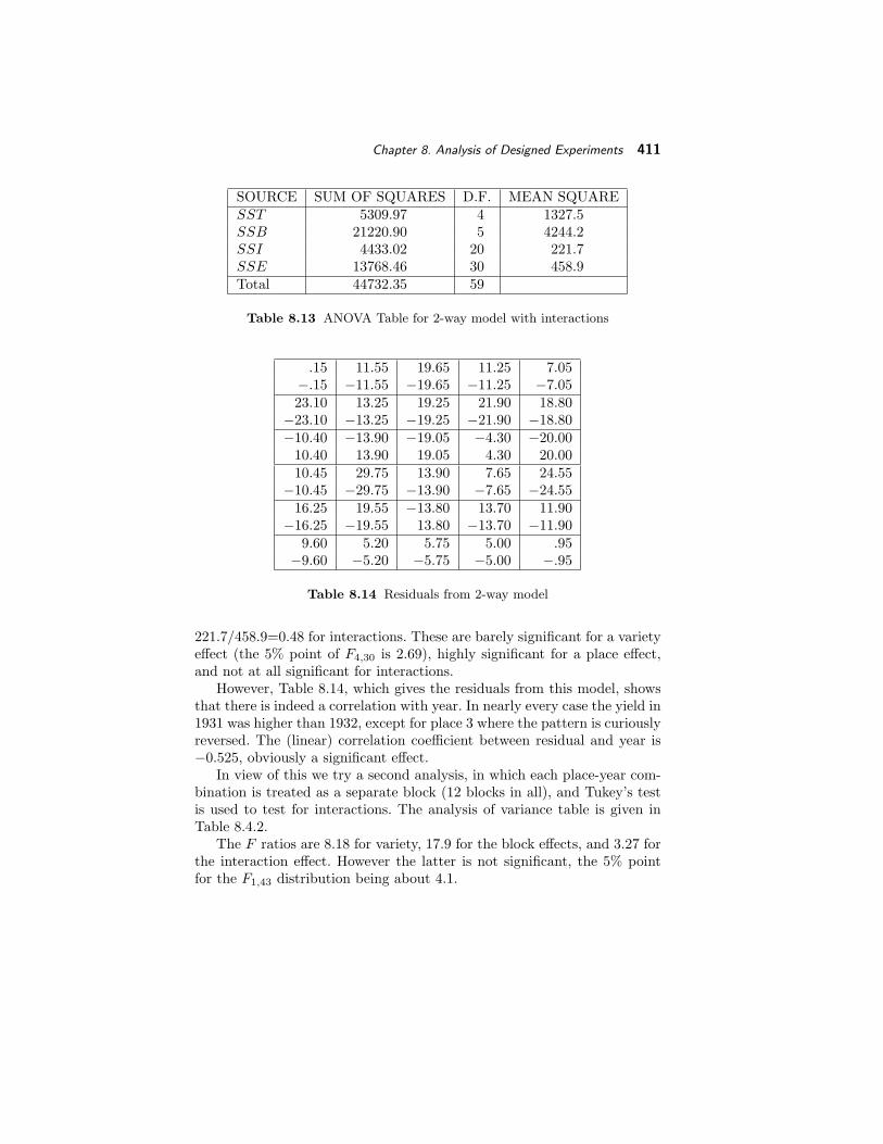
SOURCE SUM OF SQUARES D.F. MEAN SQUARESST 5309.97 4 1327.5SSB 21220.90 5 4244.2SSI 4433.02 20 221.7SSE 13768.46 30 458.9Total 44732.35 59

Table 8.13 ANOVA Table for 2-way model with interactions

.15 11.55 19.65 11.25 7.05−.15 −11.55 −19.65 −11.25 −7.0523.10 13.25 19.25 21.90 18.80

−23.10 −13.25 −19.25 −21.90 −18.80−10.40 −13.90 −19.05 −4.30 −20.00

10.40 13.90 19.05 4.30 20.0010.45 29.75 13.90 7.65 24.55

−10.45 −29.75 −13.90 −7.65 −24.5516.25 19.55 −13.80 13.70 11.90

−16.25 −19.55 13.80 −13.70 −11.909.60 5.20 5.75 5.00 .95

−9.60 −5.20 −5.75 −5.00 −.95

Table 8.14 Residuals from 2-way model

221.7/458.9=0.48 for interactions. These are barely significant for a varietyeffect (the 5% point of F4,30 is 2.69), highly significant for a place effect,and not at all significant for interactions.

However, Table 8.14, which gives the residuals from this model, showsthat there is indeed a correlation with year. In nearly every case the yield in1931 was higher than 1932, except for place 3 where the pattern is curiouslyreversed. The (linear) correlation coefficient between residual and year is−0.525, obviously a significant effect.

In view of this we try a second analysis, in which each place-year com-bination is treated as a separate block (12 blocks in all), and Tukey’s testis used to test for interactions. The analysis of variance table is given inTable 8.4.2.

The F ratios are 8.18 for variety, 17.9 for the block effects, and 3.27 forthe interaction effect. However the latter is not significant, the 5% pointfor the F1,43 distribution being about 4.1.


SOURCE SUM OF SQUARES D.F. MEAN SQUARESST 5309.97 4 1327.5SSB 31913.32 11 2901.2SSG 531.09 1 531.1SSIE 6977.97 43 162.3Total 44732.35 59

Table 8.15 ANOVA Table for Tukey’s 1-DF test

o

o

o

oo

oo

o

o

o oo o

o

oo

o

o

o

o

oo

o

o

o

o

oo

o

o

oo

ooo

o

o

o

o

o

o

o

o o

o

o

o

o

o

oo

o

oo

o

oo

o

o

o

Predicted Value

Res

idua

l

60 80 100 120 140 160

-20

-10

0

10

20

Figure 8.1 Plot of residuals vs. fitted values for barley data, 2-way modelwithout interactions

Finally, the residuals from this model have been examined with nothingsuspicious being observed. As an example, Figure 8.1 shows a plot of theresiduals against fitted values.

From this it appears that the second analysis is satisfactory. The prob-lem with the first analysis was that, by failing to treat year as a separateblock effect, the estimated variance was inflated because of what was evi-dently a significant difference between the two years.

8.5 Implementation in SAS and S-PLUS8.5.1 ANOVA in SAS

The SAS procedure ANOVA may be used to fit any version of one-wayor two-day analysis of variance, and many more different types of models.


Here is a simple example, applied to the PEMA data from Section 8.2.4.First, we create a data file ‘pema.dat’, as follows:

1 9.91 8.61 6.01 1.21 4.21 10.51 4.12 8.82 11.8

...4 8.84 8.6

Here, the data are arranged in two columns with the drug in the firstcolumn and the serum level in the second.

A SAS program to analyze these data is as follows:

options ls=64 ps=58;data pema;infile ’pema.dat’input drug serum;lserum=log(serum);run;;proc anova;class drug;model lserum=drug;means drug /lsd sheffe tukey;run;;

In the call to ‘proc anova’, the statement ‘class drug’ means that ‘drug’is being treated as a classified variable (or factor), rather than as a numer-ical variable. The ‘model’ statement then fits the one-way ANOVA model,with log serum as the response variable. The ‘means’ statement asks forcomparisons among the mean responses for each drug, with differencesevaluated according to each of the three criteria discussed in Section 8.2.7.

The output from this procedure is as follows:

The ANOVA Procedure

Class Level Information


Class Levels Values

drug 4 1 2 3 4

Number of observations 28

Dependent Variable: lserum

Sum ofSource DF Squares Mean Square

Model 3 4.88313231 1.62771077

Error 24 7.59836533 0.31659856

Corrected Total 27 12.48149764

Source F Value Pr > F

Model 5.14 0.0069

Error

Corrected Total

R-Square Coeff Var Root MSE lserum Mean

0.391230 26.66922 0.562671 2.109814

Source DF Anova SS Mean Square

drug 3 4.88313231 1.62771077


drug 5.14 0.0069

t Tests (LSD) for lserum

NOTE: This test controls the Type I comparisonwise error rate,not the experimentwise error rate.

Alpha 0.05Error Degrees of Freedom 24


Error Mean Square 0.316599Critical Value of t 2.06390Least Significant Difference 0.6207

Means with the same letter are not significantly different.

t Grouping Mean N drug

A 2.7597 7 2A

B A 2.1719 7 4BB 1.8482 7 3BB 1.6594 7 1

Tukey’s Studentized Range (HSD) Test for lserum

NOTE: This test controls the Type I experimentwise error rate,but it generally has a higher Type II error rate than REGWQ.

Alpha 0.05Error Degrees of Freedom 24Error Mean Square 0.316599Critical Value of Studentized Range 3.90126Minimum Significant Difference 0.8297


Tukey Grouping Mean N drug

A 2.7597 7 2A

B A 2.1719 7 4BB 1.8482 7 3BB 1.6594 7 1

Scheffe’s Test for lserum


NOTE: This test controls the Type I experimentwise error rate.

Alpha 0.05Error Degrees of Freedom 24Error Mean Square 0.316599Critical Value of F 3.00879Minimum Significant Difference 0.9036


Scheffe Grouping Mean N drug

A 2.7597 7 2A

B A 2.1719 7 4BB 1.8482 7 3BB 1.6594 7 1

The first part of the output reproduces the analysis of variance tablegiven earlier. The three sets of results in response to the ‘means’ state-ment all come to the same conclusion: the order of the drugs in terms ofdecreasing serum levels is 2, 4, 3, 1; drugs 2 and 4 form a common groupin the sense that they are no significantly different when judged by any ofthe three tests; similarly, drugs 4, 3 and 1 form a common group. The ac-tual critical values of t or F which determine these groupings are, however,different.

Now let us consider a two-way ANOVA without interaction, using thealloys data set of Section 8.3.2. The data are again arranged in columnformat, in a file ‘alloy.dat’:

1 1 3.061 2 3.011 3 2.84

...2 1 2.592 2 2.752 3 3.13

...4 6 2.58

A sample SAS code is now as follows:

options ls=64 ps=58;data alloy;


infile ’alloy.dat’;input bar lab strength;run;;proc anova;class bar lab;model strength=bar lab;means bar /sheffe;means lab / sheffe;run;;

The only difference from the previous example is that the are now two‘class’ variables, ‘bar’ and ‘lab’, and the model includes both of them.The ‘means’ statement asks for comparisons of both, using the Scheffe testcriterion.

Here is part of the output (edited):

Dependent Variable: strength


Model 8 2.58635000 0.32329375

Error 15 1.23343333 0.08222889


...


bar 3 0.98141667 0.32713889lab 5 1.60493333 0.32098667


bar 3.98 0.0286lab 3.90 0.0182

Scheffe’s Test for strength

...


Scheffe Grouping Mean N bar

A 3.2733 6 3A

B A 3.0083 6 1B AB A 2.8300 6 2BB 2.7450 6 4

...

Scheffe Grouping Mean N lab

A 3.4500 4 4A

B A 3.0125 4 1B AB A 3.0000 4 3B AB A 2.8900 4 2B AB A 2.8450 4 5BB 2.5875 4 6

The results of the ANOVA table are the same as given earlier, result-ing in the conclusion that both ‘bar’ and ‘lab’ are significant factors. The’means’ comparison shows that bars 3, 1 and 2 form a common group (notseparated by the Scheffe test); likewise, bars 1, 2 and 4 form a commongroup, but there are significant differences among all four groups. The cor-responding comparisons for laboratories show that laboratories 4, 1, 3, 2, 5form a common group, as do 1, 3, 2, 5, 6, but again, we reject the hypothesisthat all six laboratories are the same.

Now let us consider the Fisher barley yields example of Section 8.4.The data set is again arranged in columns, with year in column 1, place incolumn 2, variety (coded as 1–5) in columns 3, and yield in column 4:

1931 1 1 81.01931 1 2 105.41931 1 3 119.71931 1 4 109.71931 1 5 98.31932 1 1 80.7

...


1932 6 5 94.1

A possible SAS program is as follows:

options ls=64 ps=58;data fisher;infile ’fisher.dat’;input year place variety yield;run;;proc anova;class year place variety;model yield=place variety place*variety;run;;proc anova;class year place variety;model yield=year place variety;run;;

The first analysis ignores ‘year’, but treats the experiment as a two-way ANOVA with interaction — the variable ‘place*variety’ creates thisinteraction. The second analysis is slightly different from the one givenearlier — in effect a three-day analysis of variance without interactions,treating each of ‘year’, ‘place’ and ‘variety’ as a categorical variable.

The ANOVA table from the first analysis gives:


Model 29 30963.04083 1067.69106

Error 30 13767.46500 458.91550



place 5 21217.25483 4243.45097variety 4 5313.39500 1328.34875place*variety 20 4432.39100 221.61955


place 9.25 <.0001


variety 2.89 0.0387place*variety 0.48 0.9535

This analysis confirms that, analyzed as a two-way ANOVA, the inter-action term is nowhere near significant. However, the three-way analysisincluding ‘year’ yields the following:


Model 10 30327.57133 3032.75713

Error 49 14402.93450 293.93744



year 1 3796.92150 3796.92150place 5 21217.25483 4243.45097variety 4 5313.39500 1328.34875


year 12.92 0.0008place 14.44 <.0001variety 4.52 0.0035

This confirms that the ‘year’ variable is highly significant, with a p-valueof .0008, and therefore speaks strongly towards including it in the model.

8.5.2 ANOVA in R

In R, it is possible to do an analysis of variance using the lm command thatwe usually use for linear regression, after first using factor to redefine thetreatment or block variable as a factor variable. For example, to fit thePEMA data using lm, we could trydat1<-matrix(scan(’D:/r/b/s105/dat1/pema.dat’),ncol=2,byrow=T)drug<-factor(dat1[,1])lpema<-log(dat1[,2])lm1<-lm(lpema~drug)

The command summary(lm1) then produces the outputCall:lm(formula = lpema ~ drug)

Residuals:


Min 1Q Median 3Q Max-1.477082 -0.251050 -0.008663 0.471353 0.856561

Coefficients:Estimate Std. Error t value Pr(>|t|)

(Intercept) 1.6594 0.2127 7.803 4.9e-08 ***drug2 1.1003 0.3008 3.659 0.00124 **drug3 0.1888 0.3008 0.628 0.53614drug4 0.5125 0.3008 1.704 0.10128---Signif. codes: 0 *** 0.001 ** 0.01 * 0.05 . 0.1 1

Residual standard error: 0.5627 on 24 degrees of freedomMultiple R-Squared: 0.3912, Adjusted R-squared: 0.3151F-statistic: 5.141 on 3 and 24 DF, p-value: 0.006902

From this we see, in particular, that the F statistic for no treatment effecthas a p-value of about .007, implying we should reject that null hypothesis.In this analysis, the treatment effect for drug 1 is by default assumed to be0, and the analysis shows that the estimated treatment effects for drugs 2,3, 4 are respectively 1.10, 0.19 and 0.51 about that for treatment 1.

Alternatively may replace the lm command with

aov1<-aov(lpema~drug)

The command summary(aov1) then yields

> summary(aov1)Df Sum Sq Mean Sq F value Pr(>F)

drug 3 4.8831 1.6277 5.1412 0.006902 **Residuals 24 7.5984 0.3166---Signif. codes: 0 *** 0.001 ** 0.01 * 0.05 . 0.1 1

At first sight, this is not more informative. However, the aov object offersmore. For example,

> TukeyHSD(aov1)Tukey multiple comparisons of means95% family-wise confidence level

Fit: aov(formula = lpema ~ drug)

$drugdiff lwr upr p adj

2-1 1.1003440 0.2706641 1.93002384 0.00636723-1 0.1887808 -0.6408991 1.01846067 0.92213704-1 0.5125161 -0.3171638 1.34219600 0.3435628


3-2 -0.9115632 -1.7412430 -0.08188329 0.02755094-2 -0.5878278 -1.4175077 0.24185204 0.23295354-3 0.3237353 -0.5059445 1.15341521 0.7068677

This computes the mean and a 95% confidence limit for all the pairwisetreatment differences, using the Tukey pairwise comparisons procedure tocorrect for multiple comparisons. The result shows that drug 2 yields ahigher mean response than either drug 1 or drug 3; however, none of theother pairwise differences is statistically significant.

Another useful command is plot(aov1). This produces a number ofdiagnostic plots, illustrated in Figure 8.2.

The next analysis performs a similar job for the alloys data set.

x<-matrix(scan(file=’alloy.dat’),ncol=3,byrow=T)strength<-x[,3]bar<-factor(x[,1])lab<-factor(x[,2])aov2<-aov(strength~bar+lab)

This performs a two-way analysis without interactions, treating both“bar” and “lab” as factor variables. The command summary(aov2) pro-duces

Df Sum Sq Mean Sq F value Pr(>F)bar 3 0.98142 0.32714 3.9784 0.02862 *lab 5 1.60493 0.32099 3.9036 0.01820 *Residuals 15 1.23343 0.08223---Signif. codes: 0 *** 0.001 ** 0.01 * 0.05 . 0.1 1

confirming that both the lab effect and the bar effect are statistically sig-nificant. If we which to know which pairwise differences are significant, wecan use TukeyHSD(aov2) yielding

Tukey multiple comparisons of means95% family-wise confidence level

Fit: aov(formula = strength ~ bar + lab)

$bardiff lwr upr p adj

2-1 -0.1783333 -0.65549765 0.29883099 0.70812693-1 0.2650000 -0.21216432 0.74216432 0.40757214-1 -0.2633333 -0.74049765 0.21383099 0.41283403-2 0.4433333 -0.03383099 0.92049765 0.07301444-2 -0.0850000 -0.56216432 0.39216432 0.95460214-3 -0.5283333 -1.00549765 -0.05116901 0.0277449


$labdiff lwr upr p adj

2-1 -0.1225 -0.78128343 0.53628343 0.9890835....6-4 -0.8625 -1.52128343 -0.20371657 0.0074210

For the bar variable, the result shows that the bar 3 has a higher mean thanbar 4 but the other pairwise differences are not statistically significant. Forthe lab variable, most of the rows have been edited out, but only for labs4 and 6 is the difference statistically significant.

For the third example, we consider the Fisher barley yield data. In thiscase, our R program is as follows:

x<-matrix(scan(file=’fisher.dat’),ncol=4,byrow=T)yield<-x[,4]place<-factor(x[,2])year<-factor(x[,1])var<-factor(x[,3])aov3<-aov(yield~var*place)aov4<-aov(yield~year+var+place)

The first aov call is to a two-way interaction on var and place, including in-teraction (that is the meaning of writing var*place instead of var+place).The ANOVA table


var 4 5313.4 1328.3 2.8945 0.03872 *place 5 21217.3 4243.5 9.2467 2.077e-05 ***var:place 20 4432.4 221.6 0.4829 0.95347Residuals 30 13767.5 458.9---Signif. codes: 0 *** 0.001 ** 0.01 * 0.05 . 0.1 1

shows significant effects for variety and place, but no interaction.The second aov call is for a three-way analysis of variance without

interactions. In this case the ANOVA table is


year 1 3796.9 3796.9 12.9174 0.0007541 ***var 4 5313.4 1328.3 4.5192 0.0034655 **place 5 21217.3 4243.5 14.4366 1.091e-08 ***Residuals 49 14402.9 293.9---Signif. codes: 0 *** 0.001 ** 0.01 * 0.05 . 0.1 1

This shows all three main effects as statistically significant, but also amuch smaller mean squared error (293.9 against 458.9). This shows the


importance of including the year variable in the model. The correspondingdiagnostic plots are shown in Figure 8.3.

Finally, if we call the TukeyHSD(aov4) command, we get the following(most differences that are not statistically significant have been edited out):

Tukey multiple comparisons of means95% family-wise confidence level

Fit: aov(formula = yield ~ year + var + place)

$yeardiff lwr upr p adj

1932-1931 -15.91 -24.80582 -7.014178 0.0007541

$vardiff lwr upr p adj

4-1 23.816667 3.9951888 43.638145 0.01117524-2 27.075000 7.2535221 46.896478 0.00286454-3 19.025000 -0.7964779 38.846478 0.06559875-4 -15.666667 -35.4881445 4.154811 0.1830523

$placediff lwr upr p adj

2-1 43.15 20.413194 65.8868057 0.00001253-2 -30.73 -53.466806 -7.9931943 0.00271184-2 -27.14 -49.876806 -4.4031943 0.01084345-2 -55.48 -78.216806 -32.7431943 0.00000006-2 -53.19 -75.926806 -30.4531943 0.00000015-3 -24.75 -47.486806 -2.0131943 0.02553506-3 -22.46 -45.196806 0.2768057 0.05462485-4 -28.34 -51.076806 -5.6031943 0.00690636-4 -26.05 -48.786806 -3.3131943 0.0161431

This analysis confirms that both year and place are statistically significanteffects, but if our main interest were in the effect of variety, the conclusion isthat variety 4 is clearly better than varieties 1 and 2; the difference betweenvariety 4 and either of 3 or 5, although in both cases favoring variety 4, isnot statistically significant according to this analysis.


1.8 2.0 2.2 2.4 2.6 2.8

−1.

5−

1.0

−0.

50.

00.

51.

0

Fitted values

Res

idua

ls

Residuals vs Fitted

4

10

14

−2 −1 0 1 2

−3

−2

−1

01

2Theoretical Quantiles

Sta

ndar

dize

d re

sidu

als

Normal Q−Q

4

10

14

1.8 2.0 2.2 2.4 2.6 2.8

0.0

0.5

1.0

1.5

Fitted values

Sta

ndar

dize

d re

sidu

als

Scale−Location4

1014

−3

−2

−1

01

2

Factor Level Combinations

Sta

ndar

dize

d re

sidu

als

A C D Bdrug :

Constant Leverage: Residuals vs Factor Levels

4

10

14

Figure 8.2. Analysis of variance plots for PEMA data (from plot(aov1)command in R).


60 80 100 120 140 160

−40

−20

020

Fitted values

Res

idua

ls

Residuals vs Fitted

23

30 14

−2 −1 0 1 2

−2

−1

01

2Theoretical Quantiles

Sta

ndar

dize

d re

sidu

als

Normal Q−Q

23

3014

60 80 100 120 140 160

0.0

0.5

1.0

1.5

Fitted values

Sta

ndar

dize

d re

sidu

als

Scale−Location23

30 14

−2

−1

01

2

Factor Level Combinations

Sta

ndar

dize

d re

sidu

als

1932 1931year :

Constant Leverage: Residuals vs Factor Levels

23

3014

Figure 8.3. Analysis of variance plots for Fisher data, second analysis(from plot(aov4) command in R).


8.6 Exercises

1. In a round-robin experiment, the individual sample numbers ni, sam-ple means yi and sample standard deviations si are as in Table 1.

i ni yi si

1 5 37.4 5.12 5 42.3 3.13 5 49.3 2.74 8 36.1 1.7

Table 8.16 Data set for problem 8.1

It looks as though sample 3 has higher mean than the others. Dothe data in fact support that this is a significant difference? (Assumethe individual observations are all normally distributed with commonvariance σ2).

2. Ozonation as a secondary treatment for effluent following absorptionby ferrous chloride was studied for three reaction times and three PHlevels. The data in Table 8.17 were obtained for effluent decline.

PH Level7 9 10.5

23 16 14Reaction 20 21 18 13

22 15 1620 14 12

Time 40 22 13 1119 12 1021 13 11

(Minutes) 60 20 12 1319 12 12

Table 8.17 Data for Problem 8.2.

(a) Obtain the ANOVA table for a two-way analysis with interactions.

Based on the table just computed, answer the following questions:(b) Are the effects due to PH and reaction time significant?(c) Are the interactions significant?(d) In future operation, it is expected to maintain the PH level as 7,

while the reaction time will be 20 minutes for half the total time ofoperation, and 40 minutes for the other half. Obtain an estimate,


with its standard error, for the mean effluent decline, assuming (i)interactions are present, and (ii) that they are not, and commenton any noticeable differences between the two results.

3. This question is about an analysis of variance experiment, reinter-preted as a linear regression. It does not assume detailed knowledgeabout analysis of variance.A recent paper (Lee, J. and Wrolstad, R.E. (2004), Extraction of an-thocyanins and polyphenolics from blueberry-processing waste, Jour-nal of Food Science 69, No. 7, C564–C573) discussed the followingexperiment related to the extraction of juice from blueberries. Threecontrol variables were considered: temperature, level of sulfur diox-ide (SO2) and citric acid (coded as 0 or 1). Two response variableswere measured: ACY (anthocynanin) and TP (total phenolics), bothof which are considered to have beneficial health effects. The data wereas follows:

Number Temp SO2 Citric ACY TP(deg C) (ppm) Acid

1 50 0 0 27.5 55.92 50 0 1 42.6 62.63 80 0 0 50.2 71.44 80 0 1 62.4 88.85 50 50 0 92.2 307.36 50 50 1 96.5 316.47 80 50 0 97.5 420.68 80 50 1 102.2 413.89 50 100 0 90.6 386.0

10 50 100 1 82.2 337.511 80 100 0 92.1 641.012 80 100 1 91.4 684.3

Consider the model

yijk = µ + αi + βj + γk + δij + ηik + ζjk + εijk, (8.15)

where αi, i = 1, 2, βj , j = 1, 2, 3, γk, k = 1, 2 are main effectsdue to temperature, SO2 and citric acid respectively, δij , ηik, ζjk areinteraction terms, and εijk are independent N(0, σ2) errors. To makethe model identifiable, assume any of αi, βj , γk, δij , ηik, ζjk is 0 whenany of i, j, k is 1 (note that this is a different identifiability conditionfrom the ones assumed in most of the examples of this chapter).

(a) Write the model (8.15) in the form Y = Xβ + ε, where Y is thevector of responses (of dimension 12), the vector β consists of all


the non-zero unknown parameters, and X is a design matrix ofzeros and ones. (You should find that X is 12× 10.)

(b) Using SAS’s PROC REG or the “lm” command in R or S-PLUS,fit the model (8.15) to the data, where temperature, SO2 and cit-ric acid are the three factor variables and ACY is the response.Also consider possible transformations of the response and indi-cate which you prefer. (For example, you should consider both thesquare root and the log transformation, and others in the Box-Coxfamily if you have time. It is not necessary to give detailed tablesof parameter values, but state the value of the residual sum ofsquares or the estimated s, and any other statistics that are di-rectly relevant to the question.)

(c) Now using whatever transformation you selected in (b), decidewhich of the main effects and interactions is significant. (Again, Idon’t want very detailed regression output, but indicate the mainsteps of your analysis and how you did them.)

(d) Repeat the steps of (b) and (c) for the TP response variable. (It’snot necessary that the transformation of TP be the same as thatfor ACY.)

(e) Write a short report on your conclusions for the company. Recallthat the company’s objective is to choose one setting of the threecontrol variables so that both ACY and TP are high. Your reportshould indicate which settings you recommend, but should alsomake clear to what extent the differences among different possi-ble settings are statistically significant, and whether you wouldrecommend further experimentation.

Note: The proposed analysis in this question differs substantially fromthat in the paper from which the data are derived.

WILSONVILLE HIGH SCHOOL

Documents

Transcript of WILSONVILLE HIGH SCHOOL