WILLINGNESS TO PAY FOR THE HIGH COUNTRY FARM TOUR

A Thesis

by

JEFF KNICELEY

Submitted to the Graduate School

at Appalachian State University

in partial fulfillment of the requirements for the degree of

MASTERS OF BUSINESS ADMINISTRATION

December 2012

College of Business

WILLINGNESS TO PAY FOR THE HIGH COUNTRY FARM TOUR

A Thesis

by

JEFF KNICELEY

December 2012

APPROVED BY:

Dr. John C. Whitehead

Chairperson, Thesis Committee

Dr. Scott Hayward

Member, Thesis Committee

Dr. Joseph Cazier

Member, Thesis Committee

Dr. Joseph Cazier

Associate Dean for Graduate Programs and Research

Edelma D. Huntley

Dean, Cratis Williams Graduate School

Copyright by Jeff Kniceley 2012

All Rights Reserved

iv

Abstract

WILLINGNESS TO PAY FOR THE HIGH COUNTRY FARM TOUR

Jeff Kniceley

B.S., Gardner-Webb University

Chairperson: Dr. John C. Whitehead

This research aims to provide motivations for participation from the consumer

perspective in agricultural farm tours in the western portion of North Carolina. Results of a

survey taken from participants in the High Country Farm Tour will be utilized to perform

regression analysis to estimate the demand for the farm tour. By using data on stated

preferences, we estimate consumer motivation of participation based on market development,

social interaction and various pricing concepts. While much research has been completed on

the motivation of farmers to commence tourism enterprises, relatively less research is

available regarding consumer motivation in participation of such. Moreover, as motivation

for participation will vary among participants, our research will determine the effects of

changes in price of tickets and ticketing scheme on revenues. Thus, the hypothesis of the

paper will be testing the effect of prices on participation using the linear probability model.

v

Acknowledgments

I wish to express sincere appreciation to Dr. Scott Hayward and Dr. Joseph Cazier for

their assistance in the preparation of this manuscript. In addition, special thanks to Dr. John

Whitehead whose familiarity with the concepts and ideas of this study was essential in the

accumulation and analysis of the data.

vi

Table of Contents

Abstract .............................................................................................................................. iv

Acknowledgments................................................................................................................v

Section 1 Introduction ..........................................................................................................1

Rationale and Organization of Study .......................................................................1

Background ..............................................................................................................2

Conceptual Framework ............................................................................................4

Objectives and Research Question...........................................................................5

Section 2 Materials and Methods .........................................................................................5

Computations ...........................................................................................................5

Case-oriented Comparison .......................................................................................6

Section 3 Study Areas ..........................................................................................................7

Motivation for Participation .....................................................................................7

Market Segmentation ...............................................................................................8

Target Markets .........................................................................................................8

Section 4 Results ..................................................................................................................9

Regression Analysis ...............................................................................................14

Section 5 Conclusion and Recommendation .....................................................................23

References ..........................................................................................................................24

Vita .....................................................................................................................................26

1

Willingness to Pay for the High Country Farm Tour

1 Introduction

1.1. Rationale and organization of study

Blue Ridge Women in Agriculture is dedicated to strengthening the High Country’s

local food system by supporting women and their families with resources, education, and skills

related to sustainable food and agriculture. The High Country Farm Tour is hosted by the Blue

Ridge Women in Agriculture (BRWIA). In 2011, the High Country Farm Tour featured 20

farms in five counties and attracted over 500 visitors. For 2012 the Farm Tour featured 22

farms in three counties. BRWIA has hosted the High Country Farm Tour to strengthen our

local food system by connecting producers and consumers, educating the public about

sustainable food and agriculture, and providing farmers with opportunities to increase their

income. The event allows participants to tour local, sustainable farms and discover meat,

dairy, fruits, fish and veggies produced locally. The tour is self-guided and farms are located

throughout Watauga, Ashe, and Caldwell counties. Participants choose the farms they wish to

visit and visit in any order. Most farms sell their products and provide details of the history of

the farm during the tour visit. The farm tour is a major revenue source for BRWIA. BRWIA is

considering individual tickets, instead of group tickets, for the 2013 High Country Farm Tour

in order to increase revenue.

This research aims to provide motivations for participation from the consumer

perspective in agricultural farm tours in the western portion of North Carolina. A survey was

created for use to measure consumer sentiment of the High Country Farm Tour that took

place on August 4th

and 5th

, 2012. Results of the survey taken were utilized to estimate the

demand for farm tour participation. Such quantitative demand analysis as own price

elasticity of demand and its relationship to marginal and total revenue are analyzed. By

using data on stated preferences for the farm tour, it is capable of estimating consumer

motivation of participation based on market development and various pricing concepts.

The ultimate goal of the study is to determine the optimal pricing strategy for the

2013 tour season.

2

1.2. Background

Farm tourism means commercial tourism enterprises on working farms (Busby &

Rendle, 2000). Farm tourism enterprises combine the commercial constraints of regional

tourism, the nonfinancial features of family businesses, and the inheritance issues of family

farms. They have theoretical significance in regional tourism geography and economics,

family tourism business dynamics and rural diversification (Ollenburg & Buckley, 2007).

Chen, Chang and Cheng (2010) concluded that in today’s travel market, farm tourism

has gradually received attention from the masses. The momentum of this surging demand is

partially attributed to the marketing effort by concerned locals, trade associations, and the

governments that cherish their farming heritage, at the same time boosting their community

morale by rendering new experiences and activities to tourists at farm settings with small-

scale operations.

For tourism promotion agencies, farm tourism is one component of the tourism

sector, an attraction for regional travelers, but this is not necessarily how it is perceived by

the farm tourism operators themselves. Factors that motivate farm landholders to operate

tourism enterprises have considerable social and economic significance (Ollenburg &

Buckley, 2007).

Carpio, Wohlgenant, and Boonsaeng (2008) have analyzed the American 2000

National Survey on Recreation and the Environment, and found that the average farm visitor

compared with the average non visitor was more educated, had a higher family income, was

younger, and belonged to a household with more family members. They found no significant

difference between men and women in their probability to visit a farm, but male visitors have a

higher number of visits, and they found that someone living in urban areas was 5% less likely

to visit a farm than someone living in rural areas.

3

Nickerson et al. (2001) amplify the importance of looking more closely at the social

dimensions of farm businesses:

Recreation and tourism are social businesses. Farm/ranch recreation providers must

have an understanding of why people recreate, particularly if they want to stay in

business in such a specialized market. Providers must also have good interpersonal

skills to make agritourism businesses successful. We predict that farmers/ranchers who

fall into the multidimensional cluster (i.e., they are highest on social reasons for

diversification) will be most successful in recreation (p. 25-26).

The results of this review show that farm tourism has increased in popularity and that

there has been a steady increase of people visiting farm tourism enterprises. As with all forms

of niche marketing, consumer-based research is essential to the further development of farm

tourism. While there is ample research on the supply side of farm tourism, consumer research

is lacking. Specifically the interdependence of factors such as market development, travel

costs, social interaction and various costing concepts.

Visitor experiences and customer satisfaction are complex phenomena to measure and

analyze. Among marketing researchers, no single approach prevails as the best method for

analyzing gathered data (Capriello, Mason, Davis, & Crotts, 2011).

The farm experience is becoming more important, as guests want to participate and

consume farm products. More and more people are looking for new experiences, and they are

seeking connections with nature. The farm tourism business can satisfy their needs by using

distinct cultural, natural, and green characteristics of the agricultural industry. As farm-based

tourism continues to thrive, it is likely to be a viable market. In formulating effective

marketing strategies, tourism studies have investigated farm tourists’ behaviors in an effort to

understand consumers’ needs and expectations concerning farm based products and services

(Chen, Chang, & Cheng, 2010).

4

1.3. Conceptual Framework

Historically, people from the cities have turned to the countryside for recreation and

holidays. Blekesaune, Brandth, & Haugen (2010) discovered that what is new is the scope

and variety of activities and the increased demands for market-orientation, professionalism

and flexibility of the services offered, along with increased demands for quality and

competence.

Farm tourism requires management of several factors on as well as off the farm.

Each individual factor and the combination of factors need attention. Doing this in a good

way can give benefits for firms and the farm tourism sector (Forbord, Schermer, &

Griebmair, 2011).

The family farm is not only a home, but also a business. The responsibilities of

running a rural farm are driven by the cyclical nature of planting and harvesting crops, and

the daily responsibilities of caring for livestock (Trussell & Shaw, 2007). Opening a working

farm to visitors offers a secondary revenue source, but only if the farm’s capacity and market

demand is sufficient to offset the increased costs (Wilson, 2007).

Ollenburg and Buckley (2007) reported that for full-time operators, tourism is

secondary to farming, and may be abandoned if financial returns from farming improve. For

part-time farmers, tourism is a substitute for off-farm income; if farming conditions improve,

they may continue tourism but abandon off-farm employment. Retirement and lifestyle

farmers are generally unable to capitalize on improved farming conditions; tourism is their

main income even when farming conditions are good.

According to Forbord, Schermer, & Griebmair (2011), tourism products would not be

available without organization. Although such a process can take place without any formal

organization (Scott & Davis, 2007), there is little reason to believe that formal organizing

does not play a role in shaping the farm tourism sector (Forbord, Schermer, & Griebmair,

2011). Studies have shown that successful farm tourism firms work co-operatively, rather

than individualistically and competitively (Che,Veeck, & Veeck, 2005; Hill & Busby, 2002),

and that being involved with associations contributes positively to the gross income on

tourism farms (Barbieri & Mshenga, 2008).

5

1.4. Objectives and research questions

While much research has been completed on the motivation of farmers to commence

tourism enterprises; relatively less research is available regarding consumer motivation in

participation. As motivation for participation will vary among participants, this research will

consider the interdependence of factors involved in the survey in relation to social interaction

and price of tickets. Thus the hypothesis of the paper will be testing the effect of ticket price

and scheme changes using the linear probability model.

The idea is to determine the revenue maximizing group and individual ticket price.

Also, will BRWIA increase revenue if they switch from group to individual prices? To make

this determination the understanding of group size and if respondents are more or less likely to

travel in groups with individual tickets must be considered.

2 Materials and methods

2.1. Computations

A research survey was developed by faculty and students in the Department of

Economics at Appalachian State University in cooperation with Blue Ridge Women in

Agriculture. The survey questionnaire was emailed to the participants of the 2012 High

Country Farm Tour on date, with reminders on date and data. The questions were derived

from the Department of Economics’ prior experience in agriculture-related events and

surveys. Seventy-seven responses were collected out of which 64 were used in the analysis.

Survey response rate was 51% of the questionnaires sent via email. Raw data from the survey

results and data labels were created to manage the data and generate a pseudo-panel dataset, 64

individuals and 5 time periods. The 5 time periods are the demands at five different prices.

There were four dependent variables for a regression analysis: vlikely1, swlikely1,

vlikely2, swlikely2. Vlikely is equal to 1 if the respondent is very likely to pay the group or

individual ticket price. Swlikely is equal to 1 if the respondent is very likely or somewhat

likely to pay. The 1 and 2 are for group and individual tickets. If vlikely understates demand

and swlikely overstates demand the data provides bounds for a demand forecast. The models

to be estimated are vlikely1 = f(price1), swlikely 1 = f(price1), vlikely2 = f(price2),

swlikely2 = f(price2).

6

Own-price elasticity measures the responsiveness of one variable to changes in

another variable. The own price elasticity of demand for good X, denoted EQx,px, is defined

as EQx,Px=%∆Qd

x / %∆Px which is a measure of the responsiveness of the quantity demanded

of a good to a change in the price of that good. Through proper analysis of this concept we

will be able to determine the quantitative impact of price changes to farm tour participation

and revenues.

As we are aware, increasing price does not always increase revenues. There are

ranges on a linear demand curve when an increase in price will increase and decrease total

revenue. When the absolute value of the own-price elasticity (OPE) is less than 1; an

increase in price increases total revenue. When the absolute value of the own-price elasticity

(OPE) is greater than 1; an increase in price leads to a reduction in total revenue. By

utilizing the own-price elasticity, we will be able to more accurately determine the amount by

which demand will move when certain variables change. This information will allow us to

reasonably predict what effect the proposed change in ticket prices and different pricing

schemes may have on participation in the 2013 High Country Farm Tour.

2.2. Case-oriented comparison

A case study approach is a desirable research strategy when the purpose is to

understand complex social phenomena, e.g., organizational and managerial processes and the

maturation of industries (Yin, 2003). A case study gives good opportunities to bring

particular historical, cultural and geographical conditions into the analysis. Multiple cases

make it possible to consider different combinations of conditions and provide alternative

explanations for an outcome (Ragin, 1987). More specifically, a case study provides

possibilities to describe how a particular configuration of factors produces certain outcomes

(Forbord, Schermer, & Griebmair, 2011).

7

Several case studies in relation to farm tourism with various areas of concentration

were considered as outlined in Section 3 of this report. By considering these studies with the

elasticity and regression analysis, a more thorough understanding of the consumer sentiments

can be realized.

3 Study areas

3.1. Motivation for Participation

The driving force of farm tourism demand might be attributed to increased

environmental awareness according to Chen, Chang and Cheng (2010). “Experience

economy,” a phenomenon that some economists have named (Pine & Gilmore, 1999), predicts

that there is a growing interest in linking experiences with traditional products and services.

Everett and Aitchison (2008) argue that a shift in the approach to food is apparent in recent

tourism studies. This literature has traditionally focused on the role of food as economic

generator and marketing tool. The countryside is thus often conceived of as meeting consumer

demands with its envisaged authenticity, esthetical idyll, rural idyll, heritage, cuisine and small-

scale traditional food production (Hall, Mitchell, and Roberts, 2003). Basically, better

organized marketing of farm tourism, increased product diversification, and new trends in

tourist demands will continue the trend of increased numbers of visitors and increased interest

in farm tourism.

An exploratory study was conducted by Capriello, Mason, Davis and Crotts (2011) on

consumer reactions to farm visits. Three methods were applied individually to one large

qualitative database. Log likelihood comparisons of recurrent themes or word clusters in the

significant sections show that references to family, family-friendly activities and animal and

farming details were predominant themes. Also the cost of gas was mentioned frequently.

8

3.2. Market Segmentation

Developing a farm tourism business should be designed from the customer’s

perspective (Nickerson, Black, & McCool, 2001). Tourist preferences for sustainable

tourism products vary according to their demographic and socioeconomic characteristics.

Results from a large sample in the Blue Ridge National Heritage Area found preference

differences based on gender, age, education level, and income, as well as whether the tourist

was a day-tripper or overnight visitor (Stoddard, Evans, & Dave, 2008).

The marketing strategy of many tourism organizations is predicated on the theory

that tourists are heterogeneous with respect to their purchasing habits. This assumption is

often verified by data that show that certain segments of customers buy more of a product

than other segments. Often, these various market segments are defined by demographic or

socioeconomic variables such as age, education, and income (Frank & Massey, 1965).

3.3. Target Markets

Results from the research completed by Stoddard, Evans, and Dave (2008) suggest that

preferences for sustainable tourism products vary according to tourists’ demographic and

socioeconomic characteristics. The study found that tourists in various demographic and

socioeconomic groups did have diverse preferences for tourism activities. Results suggest that

promotions of music and craft activities should be directed at older, more affluent overnight

visitors. Younger visitors could be drawn by promoting outdoor activities such as hiking and

biking trails, as well as gardens, arboretums, and orchards and vineyards.

Also discovered in the study by Stoddard, Evans, and Dave (2008), the promotion for

the Blue Ridge area would best be directed toward major metropolitan areas in the southeast

United States, from North Carolina to Florida and as far west as the Mississippi River. This

study also found that the bulk of visitors originate in the southeastern United States, suggesting

that promotions for the Blue Ridge area should be directed to those living in North Carolina

and vicinity.

9

Compared to other travelers to North Carolina, visitors to the BRNHA skewed toward

being a bit older, having higher household incomes, and having attained high education levels.

Visitors of the BRNHA were few day-trippers and more overnight visitors compared to

other national heritage areas that were studied in a 2005 study. As has been the case with other

studies, this study found that women preferred crafts, men preferred outdoor activities, younger

people were more likely to choose outdoor activities, and those with high incomes preferred

gardens and trails.

4 Results

The survey was composed of several sections. The section of most interest for this

research includes the respondent answers to preferences for pricing schemes, and the

demographic and socioeconomic characteristics.

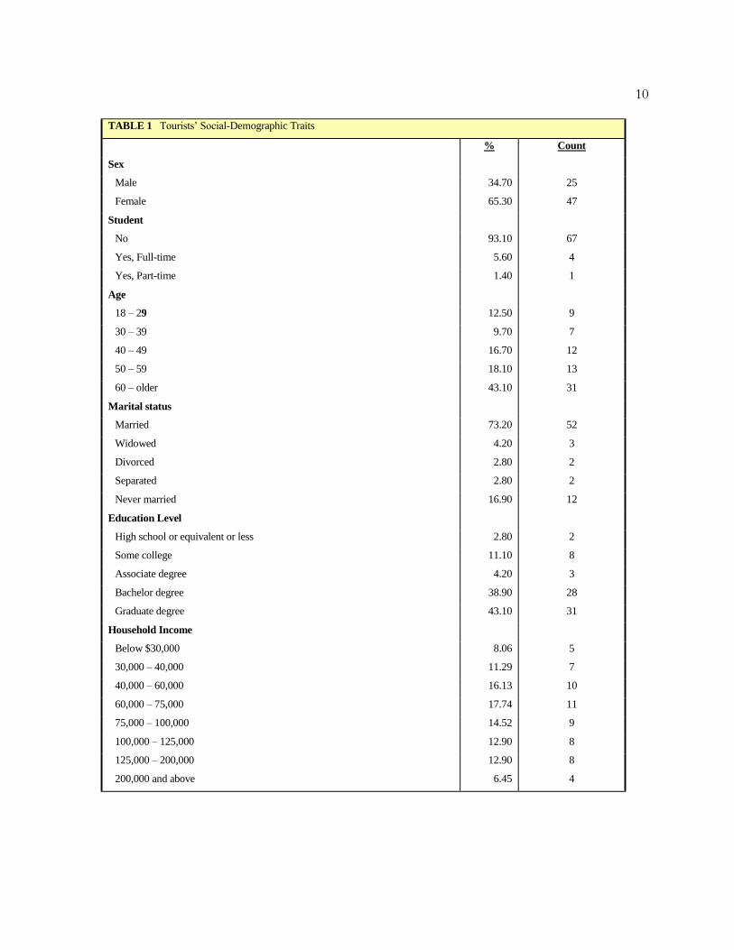
Table 1 details the respondents’ social-demographic traits. More than 65% of the

respondents were female; the majority was not considered students; the largest age category

was 60 or older; a large majority was married; more than 82% had a bachelor or graduate

degree; and the largest income section was $60,000 to $75,000 per household. In contrast,

the variables that were less represented included the age category of 18 to 39, the education

level of some college or below, and the income levels of $40,000 and below.

10

TABLE 1 Tourists’ Social-Demographic Traits

% Count

Sex

Male 34.70 25

Female 65.30 47

Student

No 93.10 67

Yes, Full-time 5.60 4

Yes, Part-time 1.40 1

Age

18 – 29 12.50 9

30 – 39 9.70 7

40 – 49 16.70 12

50 – 59 18.10 13

60 – older 43.10 31

Marital status

Married 73.20 52

Widowed 4.20 3

Divorced 2.80 2

Separated 2.80 2

Never married 16.90 12

Education Level

High school or equivalent or less 2.80 2

Some college 11.10 8

Associate degree 4.20 3

Bachelor degree 38.90 28

Graduate degree 43.10 31

Household Income

Below $30,000 8.06 5

30,000 – 40,000 11.29 7

40,000 – 60,000 16.13 10

60,000 – 75,000 17.74 11

75,000 – 100,000 14.52 9

100,000 – 125,000 12.90 8

125,000 – 200,000 12.90 8

200,000 and above 6.45 4

11

Of the respondents a moderate percentage had participated in previous High Country

Farm Tours (Table 2).

Table 2 Tourist’s Participation Level

Year % Count

2012 100.00 72

2011 23.70 18

2010 18.40 14

2009 13.20 10

Approximately 95% stated they were either moderately satisfied or extremely satisfied

with their experience with the 2012 tour. As for the respondents’ social interaction traits, only

10% traveled alone while the remaining 89% traveled within a group (Table 3).

Table 3 Group Size

% Count

1 9.72 7

2 50.00 36

3 13.89 10

4 18.06 13

5 6.94 5

6 0.00 0

More than 6 1.39 1

12

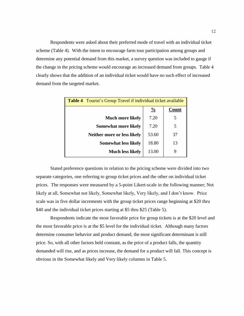
Respondents were asked about their preferred mode of travel with an individual ticket

scheme (Table 4). With the intent to encourage farm tour participation among groups and

determine any potential demand from this market, a survey question was included to gauge if

the change in the pricing scheme would encourage an increased demand from groups. Table 4

clearly shows that the addition of an individual ticket would have no such effect of increased

demand from the targeted market.

Table 4 Tourist’s Group Travel if individual ticket available

% Count

Much more likely 7.20 5

Somewhat more likely 7.20 5

Neither more or less likely 53.60 37

Somewhat less likely 18.80 13

Much less likely 13.00 9

Stated preference questions in relation to the pricing scheme were divided into two

separate categories, one referring to group ticket prices and the other on individual ticket

prices. The responses were measured by a 5-point Likert-scale in the following manner; Not

likely at all, Somewhat not likely, Somewhat likely, Very likely, and I don’t know. Price

scale was in five dollar increments with the group ticket prices range beginning at $20 thru

$40 and the individual ticket prices starting at $5 thru $25 (Table 5).

Respondents indicate the most favorable price for group tickets is at the $20 level and

the most favorable price is at the $5 level for the individual ticket. Although many factors

determine consumer behavior and product demand, the most significant determinant is still

price. So, with all other factors held constant, as the price of a product falls, the quantity

demanded will rise, and as prices increase, the demand for a product will fall. This concept is

obvious in the Somewhat likely and Very likely columns in Table 5.

13

Table 5 Pricing Scheme

Group

Ticket

Prices Not Likely

Somewhat

not likely

Somewhat

likely

Very

likely

I don’t

know

$20 0.0% (0) 0.0% (0) 10.9% (7) 84.4% (54) 4.7% (3)

$25 0.0% (0) 4.6% (3) 15.4% (10) 76.9% (50) 3.1% (2)

$30 10.3% (6) 17.2% (10) 44.8% (26) 25.9% (15) 1.7% (1)

$35 26.3% (15) 43.9% (25) 22.8% (13) 3.5% (2) 3.5% (2)

$40 55.4% (31) 32.1% (18) 7.1% (4) 1.8% (1) 3.6% 92)

Single

Ticket

Prices Not Likely

Somewhat

not likely

Somewhat

likely

Very

likely

I don’t

know

$5 1.6% (1) 0.0% (0) 8.2% (5) 88.5% (54) 1.6% (1)

$10 3.1% (2) 1.6% (1) 25.5% (16) 68.8% (44) 1.6% (1)

$15 11.9%(7) 28.8% (17) 28.8% (17) 25.4% (15) 5.1% (3)

$20 43.1%(25) 32.8% (19) 10.3% (6) 10.3% (6) 3.4% (2)

$25 71.4% (40) 16.1% (9) 5.4% (3) 3.5% (2) 3.6% (2)

14

4.1. Regression Analysis

By using ordinary least squares regression linear probability models we are estimating

by regressing vlikely and swlikely on the admission price. Vlikely is equal to one of the

respondent is very likely to participate in the farm tour, zero otherwise. Swlikely is equal to one

if the respondent is somewhat likely and very likely to participate in the farm tour, zero

otherwise. The vlikely and swlikely are treated as subgroups to be used as upper and lower-

level bounds. The average of the subgroups will then be used to determine the optimal pricing

scheme per group.

Utilizing the ordinary least squares method, the linear probability model is estimated: y

= a + bP, where a and b are regression coefficients, where the expected sign on the coefficients

are a>0, b<0. The data allows the estimation of demand functions for all four data sets of

vlikely1 = f(price1), swlikely 1 = f(price1), vlikely2 = f(price2), swlikely2 = f(price2).

This method of estimation results in four demand curves with which, through inverting

the demand function, provides the means to calculate total revenue, marginal revenue and own-

price elasticity for both the group and individual ticket pricing schemes.

The regression analysis not only provides means for essential calculations, it also

provides information as to the significance and reliability of the data. The t-statistic of a

parameter estimate is the ratio of the value of the parameter estimate to its standard error. The

standard error of each estimated coefficient is a measure of how much each estimated

coefficient would vary in regressions based on the same underlying true demand relation, but

with different observations (Baye, 2010). A general rule for the t-statistic is the absolute value

being greater than 2, the higher the better.

The R-squared statistic tells the fraction of the total variation in the dependent variable

that is explained by the regression. The general meaning is that the R-squared function

explains the percentage of the total variations across the sample. The closer the R-squared is to

1, the greater the overall fit of the estimated regression equation is to the actual data (Baye,

2010).

15

While the R-squared provides a guide for overall fit, there is no universal rule for

determining how large the number should be to indicate a good fit. The F-statistic does not

suffer this deficiency. The F-statistic provides a measure of the total variation explained by the

regression relative to the total unexplained variation. The greater the F-statistic, the better the

overall fit of the regression lines though the actual data.

The value of R-squared ranges from 0 to 100 percent. This model explains 48.6% of

the variation in the dependent variable of Group Very Likely and 43.9% of the dependent

variable of Group Somewhat Likely. The Individual Very Likely R-squared value is 40.1%

and the Individual Somewhat Likely is 42.2%. R-squared tells how well the regression line

approximates the real data. A high value of R2 is obviously important in forecasting situations.

F-statistic provides a measure of the total variation explained by the regression relative

to the total unexplained variation. The greater the F-statistic, the better the overall fit of the

regression line thorough the actual data. The values of 301.134 and 248.405 for the Group

Very Likely and Group Somewhat Likely respectively, indicate a significant level of fit. The

Table 6 Regression Results

Group Individual

Very Likely

Somewhat

Likely

Very Likely

Somewhat

likely

Constant

(t-stat)

1.791

(21.22)

1.95

(21.42)

1.013

(20.65)

1.205

(24.12)

Price

(t-stat)

-0.0475

(-17.35)

-0.0466

(-15.76)

-0.0431

(-14.59)

-0.0459

(-15.25)

R2 .486 .439 .401 .422

F-statistic 301.134 248.405 212.805 232.614

16

Individual Very Likely F-statistic is 212.805 and the Individual Somewhat Likely result is

232.614. These results also represent a significant level of fit.

The t-statistic describes how many standard deviations away the calculated value of

the coefficient is from zero. This is significant because if the coefficient for a variable is not

different from zero, then the variable doesn’t really affect the predicted value. The t-statistics

for our constant are all above 20. The absolute values of the t-statistics for price range from

14.59 to 17.25. Since they are both well beyond our general rule of 2.0, we can have some

confidence in making observations based on these results.

The sign associated with slope tells us that quantity decreases by .0475 units when

price increases by one unit for the Group Very Likely model. The Group Somewhat Likely

model indicates that quantity will decrease by .0466 units when price increases by one unit.

For the Individual Very Likely model, quantity will decrease by .0431 for price unit increase

and quantity will decrease by .0459 units for each price unit increase in the Individual

Somewhat Likely model.

Based on these results we can determine that price has a significant negative impact

on quantity. As price increases, quantity will decrease respectively.

17

As detailed in Table 6 above, the regression analysis gives us the coefficients of the

intercept and price that allows us to determine the demand function. The formula Q = 1.791 –

0.0475P gives us the demand curve for the vlikely group data set. The same demand functions

are created using the coefficients of the intercept and price for each of the remaining three data

sets.

Figure 1 shows the inverse demand curve for the demand model of vlikely1 = f(price1)

while Figure 2 represents the inverse demand curve for the demand model of swlikely1 =

f(price1).

Figure 1 Inverse Demand Curve for vlikely1 = f(price1)

Figure 2 Inverse Demand Curve for swlikely1 = f(price1)

0

5

10

15

20

25

30

0.00 0.50 1.00 1.50 2.00

Pri

ce

Quantity

Vlikely - Group

0

5

10

15

20

25

30

35

0.00 0.50 1.00 1.50 2.00 2.50

Pri

ce

Quantity

SwLikely - Group

18

Figure 3 shows the inverse demand curve for the demand model of vlikely2 = f(price2)

and figure 4 represents the inverse demand curve for the demand model of swlikely2 =

f(price2).

Figure 3 Inverse Demand Curve for vlikely2 = f(price2)

Figure 4 Inverse Demand Curve for swlikely2 = f(price2)

To find the total revenue (TR) and marginal revenue (MR) for this data set, we use the

inverse demand function as P = 37.697 – 21.053Q.

0

5

10

15

20

25

30

0 0.5 1 1.5

Pri

ce

Quantity

SwLikely - Individual

0

2

4

6

8

10

12

14

16

0.00000 0.20000 0.40000 0.60000 0.80000 1.00000 1.20000

Pri

ce

Quantity

Vlikely - Individual

19

To determine which pricing scheme provides the greatest total revenue it is necessary

to solve the following equation Total Revenue (TR) = Price (P) * Quantity (Q) for each price

level. Marginal revenue is the change in total revenue due to a change in quantity. This

relationship among the changes in price, elasticity, and total revenue is called the total

revenue test.

Demand is elastic if the absolute value of the own price elasticity (OPE) is greater than

1. Demand is inelastic if the absolute value of the own price elasticity is less than 1. If

demand is elastic, an increase (decrease) in price will lead to a decrease (increase) in total

revenue. If demand is inelastic, an increase (decrease) in price will lead to an increase

(decrease) in total revenue. Total revenue is maximized at the point where demand is unitary

elastic (Baye, 2010).

Table 7 represents the revenue analysis for the group pricing scheme while Table 8

summarizes the revenue analysis for individual pricing scheme. Notice in Table 7 and Table 8

that the absolute value of the OPE gets larger as price increases. Thus, the OPE of demand

varies along a linear demand curve.

The price-quantity combination that maximizes total revenue in Table 7 and Table 8 is

at the point where the OPE equals 1, which is also the point that MR = 0. Revenue is

maximized at the quantity that makes MR = 0. Since the vlikely calculation may understate

expected demand and the swlikely calculation may overstate it, the correct forecast is likely in

between.

20

Table 7 Regression Analysis – Simulation

Group - Vlikely

Demand Function Q= 1.790625 -0.0475 P

Inverse Demand P= 37.69737 -21.05263 Q

P Q TR MR OPE

0.00 1.79063 0.00 ---- ----

5.00 1.55313 7.76563 7.766 0.133

10.00 1.31563 13.15625 5.391 0.153

15.00 1.07813 16.17188 3.016 0.361

19.01 0.88765 16.87423 0.000 1.016

20.00 0.84063 16.81250 -0.061 1.022

25.00 0.60313 15.07813 -1.734 1.130

Group - Swlikely

Demand Function Q= 1.95 -0.046562 P

Inverse Demand P= 41.87919 -2147651 Q

P Q TR MR OPE

0.00 1.95000 0.00 ---- ---

5.00 1.71719 8.58594 8.586 0.119

10.00 1.48438 14.84375 6.258 0.136

15.00 1.25156 18.77344 3.930 0.314

20.00 1.01875 20.37500 1.602 0.558

21.01 0.97172 20.41588 0.000 1.006

25.00 0.78594 19.64844 -0.766 1.015

21

Table 8 Regression Analysis – Simulation

Individual – Vlikely

Demand Function Q= 1.0125 -0.043125 P

Inverse Demand P= 23.47826 -23.18841 Q

P Q TR MR OPE

0.00 1.01250 0.00 --- ---

5.00 0.79688 3.98438 3.984 0.213

10.00 0.58125 5.81250 1.828 0.271

11.00 0.53813 5.91938 0.107 0.742

11.76 0.50535 5.94292 0.000 1.002

11.77 0.50492 5.94289 0.000 1.004

15.00 0.36563 5.48438 -0.459 1.005

Individual – Swlikely

Demand Function Q= 1.790625 -0.0475 P

Inverse Demand P= 37.69737 -21.05263 Q

P Q TR MR OPE

0.00 1.20469 0.00 0.00 0.00

5.00 0.97500 4.87500 4.875 -0.764

10.00 0.74531 7.45313 2.578 0.236

15.00 0.51563 7.73438 0.281 0.616

15.01 0.51517 7.73264 -0.002 1.336

20.00 0.28594 5.71875 -2.012 1.347

25.00 0.05625 1.40625 -4.313 3.213

22

With the vlikely and swlikely acting as subgroups used as upper and lower-level limits,

the average of the subgroups will be used to determine the optimal pricing scheme per pricing

concept. Table 9 details the results of both categories as bounds for a demand forecast. Based

on the survey responses only, and not the total demand for the farm tour, the total individual

demand calculates to 165, the average party size multiplied by the number of groups, with

group demand at 64.

By averaging the data sets, the optimal pricing level is determined for each pricing

concept in addition to the corresponding quantity percentage. The correlated percentage of

quantity is multiplied by the appropriate demand category, group, or individual, to determine

overall quantity for the data set. This quantity is then multiplied to the optimal price to

determine the TR for the respective pricing concept.

Table 9 Summary / Recommendation

Average Party Size 2.578

Total Demand from Sample 165

Total Number of Groups 64

BOUNDS

With Projected Price – VL P Q TR

Group (88.77%) 19.01 56.8096 1,079.95

Individual (50.54%) 11.76 83.38275 980.58

With Projected Price –SwL P Q TR

Group (97.17) 21.01 62.19008 1,306.61

Individual (52.52%) 15.01 85.00305 1,275.90

OPTIMAL REVENUE P Q TR

Group (90%) 20.00 57.6 1,152.00

Individual (50%) 12.50 82.5 1.031.25

23

5. Conclusion and Recommendation

The BRWIA is considering changing from a group pricing concept to an individual

pricing concept for the 2013 High Country Farm Tour. This research was to determine the

optimal pricing scheme that would maximize the BRWIA’s total revenue for the 2013 season.

Through the utilization of ordinary least squares regression linear probability models it

is estimated the group pricing scheme would optimize total revenue, given the demand remains

as current.

The mixture of the economic data analyzed within this study and the case studies noted

throughout highlights the necessity of additional research into the effect of demand shifters

within the specific market. Particular focus should be on the interdependence of factors such

as market development, relationship with other local farm tours, the effect of travel costs,

demographics and socioeconomic factors. It would also be beneficial to complete a sensitivity

analysis for changes in group size with the change in pricing scheme or with the addition of a

pricing concept mix.

Continued research should be prepared to determine the proper market segment and

target for the farm tour industry. While the case studies analyzed within this research assisted

in generalizing certain target areas, additional research is necessary to make the targeted market

segment more specific.

As concluded in Table 9 the group pricing concept allows for greater total revenue than

the individual pricing scheme. Therefore it is recommended that the BRWIA 2013 High

Country Farm Tour maintain the group pricing concept.

24

REFERENCES

Barbieri, C., & Mshenga, P.M. (2008). The role of the firm and owner characteristics on the

performance of agritourism farms. Sociologia Ruralis, 48(2), 166-183.

Baye, M.R. (2010). Managerial Economics and Business Strategy. New York, N.Y.:

McGraw-Hill Irwin.

Blekesaune, A., Brandth B., & Haugen, M.S. (2010). Visitors to Farm Tourism Enterprises in

Norway, Scandinavian. Journal of Hospitality and Tourism, 10(1), 54-73.

Busby, G., & Rendle, S. (2000). The transition from tourism on farms to farm tourism.

Tourism Management, 21(8), 635-642.

Capriello, A., Mason, P.R., Davis, B., & Crotts, J.C. (2011). Farm Tourism experiences in

travel reviews: A cross-comparison of three alternative methods for data analysis.

Journal of Business Research, 09, 1-8.

Carpio, E.E., Wohlgenant, M.K., & Boonsaeng, T. (2008). The demand for agrotourism in the

United States. Journal of Agricultural and Resource Economics, 33(2), 245-269.

Che, D., Veeck, A., & Veeck, G. (2005). Sustaining production and strengthening the

agritourism product: linkages among Michigan agritourism destinations. Agriculture

and Human Values, 22(2), 225-234.

Chen, J.S., Chang, L, & Cheng, J. (2010). Exploring the Market Segments of Farm Tourism in

Taiwan. Journal of Hospitality Marketing and Management, 19(4), 309-325.

Everett, S., & Aitchison, C. (2008). The role of food tourism in sustaining regional identity: A

case study of Cornwall, South West England. Journal of Sustainable Tourism, 16(2),

150-167.

Forbord, M., Schermer, M., & Griebmair, K. (2011). Stability and variety – Products,

organization and institutionalization in farm tourism. Tourism Management, 33, 895–

909.

Frank, R.E., & Massey, W.F. (1965). Market segmentation and the effectiveness of a brand’s

price and dealing policies. Journal of Business 38(2), 186-200.

25

REFERENCES cont.

Hall, D., Mitchell, M., & Roberts, L. (2003). Tourism and the countryside: Dynamic

relationships. In D. Hall, G. Rozman, & M. Mitchell (Eds.), New Directions in Rural

Tourism (pp. 3-15). Aldershot:Ashgate.

Hill, R., & Busby, G. (2002). An inspector calls: farm accommodation providers’ attitudes to

quality assurance scheme in the county of Devon. The International Journal of Tourism

Research, 4(6), 459-478.

Nickerson N., Black, R., & McCool, S. (2001). Agritourism: Motivations behind farm/ranch

business diversification. Journal of Travel Research, 401 (1), 19-26.

Ollenburg, C., & Buckley, R. (2007). Stated Economic and Social Motivations of Farm

Tourism Operators. Journal of Travel Research, 45, 444-452.

Pine, J.P. II, & Gilmore, H.H. (1999). The experience economy: Work is theatre and every

business a state. Cambridge, MA: HBS Press Book.

Ragin, C.C. (1987). The comparative method: Moving beyond qualitative and quantitative

strategies. Berkeley: University of California Press.

Scott, W.R., & Davis, G.F. (2007). Organizations and organizing: Rational , natural, and open

system perspectives. Upper Saddle River, N.J.: Pearson Education.

Stoddard, J. E., Evans, M.R., & Dave, D.S., (2008). Sustainable Tourism: The Case of the Blue

Ridge National Heritage Area. Cornell Hospitality Quarterly, 49, 245-257.

Trussell D., Shaw, S. (2007). Daddy’s gone and he’ll be back in October: Farm women’s

experiences of family leisure. Journal of Travel Research, 39(2), 366-87.

Wilson L. (2007). The family farm business? Insights into family, business and

ownership dimensions of open-farms. Leisure Study, 26(3), 357-74.

Yin, R.K. (2003). Case study research: Design and methods. Thousand Oaks, CA:

Sage.

26

Vita

Jeff Kniceley was born in Sutton, West Virginia, to Nolan and Mary Jo Kniceley. He

graduated from Braxton County High School in May 1985. Upon graduation he moved to

Shelby, North Carolina to pursue his education. He graduated Alpha Sigma Lambda and

Summa Cum Laude from Gardner-Webb University with a Bachelor of Science degree in

December 2008. He began his studies at Appalachian State University in the fall of 2010 and

was awarded his Master of Business Administration with a concentration in Economics in

December 2012.

Mr. Kniceley is a member of The International Honor Society Beta Gamma Sigma. He

resides in Shelby, North Carolina with his wife and three children.