WIDER Working Paper 2017/93

WIDER Working Paper 2017/93

Are there different spillover effects from cash transfers to men and women?

Impacts on investments in education in post-war Uganda

Margherita Calderone*

April 2017

* University of Turin, Italy, [email protected]

This study has been prepared within the UNU-WIDER project on ‘Gender and Development’.

Copyright © UNU-WIDER 2017

Information and requests: [email protected]

ISSN 1798-7237 ISBN 978-92-9256-317-2

Typescript prepared by Merl Storr.

The United Nations University World Institute for Development Economics Research provides economic analysis and policy advice with the aim of promoting sustainable and equitable development. The Institute began operations in 1985 in Helsinki, Finland, as the first research and training centre of the United Nations University. Today it is a unique blend of think tank, research institute, and UN agency—providing a range of services from policy advice to governments as well as freely available original research.

The Institute is funded through income from an endowment fund with additional contributions to its work programme from Denmark, Finland, Sweden, and the United Kingdom.

Katajanokanlaituri 6 B, 00160 Helsinki, Finland

The views expressed in this paper are those of the author(s), and do not necessarily reflect the views of the Institute or the United Nations University, nor the programme/project donors.

Abstract: This paper looks at the spillover effects of grants under the Youth Opportunities Programme (YOP) on human capital investments in conflict-affected Northern Uganda. The YOP grant was primarily aimed at providing start-up money to groups of underemployed young people, and in practice worked similarly to an unconditional cash transfer. It kept a gender balance by mandating that groups should be at least one third female. Overall, the intervention had a significant impact on education-related expenditures, increasing them by 11–15 per cent (US$17–23) in the shorter and longer term (i.e. after two and four years). However, the educational expenditures of women did not increase. Female recipients seem not to have spent more on education, at least in part because of redistributive pressures such as probable financial requests from other members of their YOP group. These findings are relevant for future designs of group eligibility rules and for targeting of cash transfers.

Keywords: cash transfers, spillover effects, household consumption, education expenditures JEL classification: J16, O1

Acknowledgements: This research received support from the UNU-WIDER ‘Gender and Development’ project, and from the European Union’s Seventh Framework Programme under grant agreement 609402 (‘2020 Researchers: Train 2 Move’ T2M Project). I am grateful to Nathan Fiala for sharing the data and providing comments on the first draft. I thank Martina Björkman Nyqvist, Siwan Anderson, and numerous seminar participants for insightful comments. All errors and opinions are mine.

mailto:[email protected]

https://www.wider.unu.edu/node/379

1

1 Introduction

Low levels of investment in productive activities and human capital often constitute a key constraint on households’ escape from poverty. In conflict-affected and post-conflict countries, investments are limited even further by detrimental economic shocks and by lower expected returns on capital and education. Hence many development projects, especially reconstruction interventions, are directed to support the investments of the poor.

Cash transfers in particular are aimed at alleviating poverty in the short run by providing money, and at breaking the intergenerational transmission of poverty by inducing investments in child education and health—usually through conditionalities. Evidence from numerous countries suggests that these programmes are generally successful in reaching their primary objectives, i.e. increases in school enrolments or the use of health services (see Fizbein et al. 2009 for a review, and Saavedra and Garcia 2012 for a recent meta-analysis). However, their focus on the human capital accumulation of the young has led to some criticism because they might miss opportunities to alter productive activities and have broader effects on graduation from poverty. Indeed, most cash transfers have been shown to have little impact on work incentives and adult labour supply (see Alzua et al. 2013 and Banerjee et al. 2015 for comparable results from different countries).

In this sense, the Youth Opportunities Programme (YOP) represents a remarkable success story. Supported by the government of Uganda and the World Bank, the YOP was a grant that provided start-up money to groups of underemployed young people from the post-conflict north. Blattman et al. (2014a) demonstrate that the programme did substantially increase productive assets, along with work hours, earnings, and the probability of practising a skilled trade. This paper adds to the literature by looking at the spillover effects of the YOP on investments in human capital, particularly educational expenditures.

First, the effect of the YOP on educational outcomes is an empirical question, which is relevant for understanding the overall desirability of such interventions. For instance, Shah and Steinberg (2015) present mixed results regarding the impact of the National Rural Employment Guarantee Act, a large workfare programme, on human capital in India: the effect was positive for children aged two to eight (significantly positive for children aged two to four), but negative for adolescents. Similarly, Kugler et al. (2015) show that a vocational training programme for disadvantaged youth in Colombia increased human capital accumulation—including formal education—of training participants and their family members, but only for male participants.

Second, the spillover effects of the YOP might differ by gender, since women in developing countries have to face stronger constraints than men (Cho et al. 2013) that might limit their capacity to benefit from the full range of positive externalities of a programme.

In this paper, I show that the YOP grant was effective in increasing education-related expenditures, which grew by 11–15 per cent (US$17–23) in the shorter and longer term (i.e. after two and four years). The intervention also increased subjective education-related outcomes by six per cent overall (by eight per cent for men). Interestingly, the results do not seem to be driven by a direct income effect from the money injection, since the size of the grant received influenced only food expenditures. More specifically, men assigned to receive the grant increased total educational expenditures by 21–24 per cent (US$32) after both two and four years, whereas total educational expenditures of female recipients did not increase. The effect for men is driven by a growth in expenditures on their own children and family members. Women did not change their family

2

spending patterns; however, they did increase their expenditures for non-family members by 90–95 per cent after two years.

These gender-differentiated effects might be due to different reasons. One hypothesis is that women did not increase investment in human capital because they had already met their optimal level of expenditure on family education. The heterogeneous effects suggest this is not the case, since better-educated women did manage to spend significantly more on the education of their own children and family members. Another hypothesis is that women could not invest more in their family’s education because after receipt of the grant they were subject to stronger redistributive pressures. It was mandatory for one third of the members of YOP groups to be female. Hence the pressures that women suffered might have included financial requests from the other members of their YOP group. The analysis of the heterogeneous effects offers evidence in support of this hypothesis. Women who were badly matched to their YOP group, i.e. women who belonged to groups with higher human capital disparity or who, from the time of the baseline, were dissatisfied with their group, did spend substantially more on transfers outside their households.

These results are in line with evidence in Blattman et al. (2014a) indicating that despite a significant increase in earnings, the social position of women did not improve. On the contrary, in the shorter term their antisocial behaviours increased, and in the longer term their participation in groups decreased. This suggests that forcing men to team up with women in the YOP groups might have impeded full attainment of the stated goal of gender balance.

These findings are relevant for the design of group eligibility rules and the targeting of cash transfers, and they pave the way for further research focusing on the role of gender composition in group dynamics. One paper on this topic by Berge et al. (2016) proposes a laboratory experiment to study the ability to collaborate and make risk-taking decisions among groups of microfinance clients in Tanzania. The authors show that female groups are more able to collaborate and find common solutions to challenges than mixed (or male) groups.

This study also contributes to the recently growing literature on the constraints that women face when making decisions in developing countries. One strand of this literature focuses on gender discrimination and highlights a series of negative social biases women have to bear. Cho et al. (2013) claim that women in Malawi who participate in training are constrained by family obligations and penalized by trainers, who are more likely to provide financial help and paid work to men than to women after training. Similarly, BenYishay et al. (2016) show that even though women learn and retain information about new agricultural technologies better, they are not as successful as men at convincing others to adopt those technologies, because other farmers perceive them as less able communicators. Another strand of the literature investigates the extent of redistributive pressures, and while it does not have gender as its primary focus, it does underline stark gender differences. In their important paper, Jakiela and Ozier (2016) demonstrate that women in rural Kenya are significantly burdened by social pressures to share their income with their kin and neighbours. They estimate that women’s income is ‘taxed’ at a rate around four per cent, or almost eight per cent when kin can observe income directly. Focusing on family pressures in Uganda, Quisumbing et al. (2011) show that wives’ assets are less insured against shocks than husbands’ assets. Along the same lines, Fiala (2015a) suggests that women in Uganda feel pressure from husbands to invest their money in other household businesses: women that receive loans do not profit from them, whereas the income of their spouses increases. Boltz et al. (2015) offer evidence from urban Senegal that women exhibit high willingness to pay to hide money and escape redistributive pressures. Interestingly, women’s willingness to hide increases with the number and strength of social ties (such as always having lived in the community), while almost the reverse is

3

found for men. In addition, the authors show that lottery winners that manage to transfer less to others (private winners) do spend more on private items and health.

This paper is also based on the literature analysing the consumption impacts of cash transfers, whether conditional (Attanasio et al. 2011 on Colombia; Cruz and Ziegelhöfer 2014 on Brazil; Gertler et al. 2012 on Mexico; Macours et al. 2012 on Nicaragua, with a focus on food consumption and child nutrition) or unconditional (Bazzi et al. 2015 on Indonesia; Haushofer and Shapiro 2016 on Kenya; Schady and Rosero 2008 on Ecuador). This study is also linked to the literature on the impact of aid programmes in Uganda, a country with one of the youngest populations in the world (48 per cent of its citizens are under the age of 151). Recent evidence suggests that development programmes targeted at the country’s youth have been successful in tackling a range of issues from lack of skills to risky health behaviours, child mortality, and underinvestment in education (Bandiera et al. 2015; Björkman and Svensson 2009; Blattman et al. 2014a; Karlan and Linden 2014).

The rest of the paper is organized as follows. Section 2 reviews the literature on cash transfers and theoretical models of collective consumption, highlighting the YOP features that are distinctive with respect to the usual cash transfer programmes. Section 3 describes the context of the intervention, along with details about it and its impact evaluation. Section 4 provides further information on the data and descriptive statistics. Section 5 explains the identification strategy and presents the results. Finally, Section 6 discusses the findings and offers concluding remarks.

2 Cash transfers and intrahousehold decision-making: a literature review

A number of articles studying intrahousehold bargaining show that resources under the mother’s control have a more beneficial impact on a child’s well-being. As Duflo (2012) summarizes, various influential papers since the 1990s have suggested that income or assets in the hands of women rather than men are associated with stronger positive effects on child health (Thomas 1990) and with increased percentages of household budgets being spent on family health and food nutrients (Thomas 1993). Maluccio and Quisumbing (2003), Duflo (2003), and Duflo and Udry (2004) have offered additional empirical evidence supporting such findings. This literature provided a rationale for directing cash transfers to mothers.

More recent papers looking at the effects of Conditional Cash Transfers (CCTs) show that the extra money in the hands of women is indeed well spent. For instance, Rubalcava et al. (2009) study the impact of Progresa in Mexico and show that beneficiary women who have resources under their control are more likely to spend them on small livestock, improved nutrition, and child goods (particularly clothing). Similarly, De Brauw et al. (2014) find that in Brazil’s urban areas the Bolsa Familia CCT had significant impacts on the decision-making power of women, as well as on children’s school attendance, child health expenditures, and household purchases of durable goods. This strand of literature generally uses the collective model to explain the mechanisms behind the effects of targeting cash transfers at women (e.g., Attanasio and Lechene 2002, 2014). In a unitary model, cash transfers would affect household decisions only through the impact they have on total income and budget constraints. In a collective model, targeted transfers might also

1 Niger is the only country with a higher number, at 50 per cent (World Bank 2014).

4

change the balance of power within the household, and as a consequence the allocation of resources.2

However, transferring cash to women does not necessarily imply an increase in women’s power over household resources. Analysing the impact of Progresa, Handa et al. (2009) find effects only on women’s capacity to spend their own cash, and not on other decision-making spheres. De Brauw et al. (2014) show that the impact of Bolsa Familia on women’s bargaining power was substantially heterogeneous and not significant in rural areas. Yoong et al. (2012) review the literature on transfers to men and women and find no consensus on whether CCTs increase women’s decision-making power. Almås et al. (2015) argue that previous inconclusive results might be due to measurement issues, while Peterman et al. (2015) test different women’s decision-making indicators across three countries and still show mixed evidence.

In this regard, it is important to note that the YOP grant was not targeted at individuals directly, but at groups that had the responsibility to share the cash among male and female members. Hence it is likely that group structure and matching played a role in influencing the effectiveness of the grant. For instance, Arcand and Fafchamps (2012) find that community-based organizations in West Africa tend to exclude less fortunate members of society, such as female-headed households, from the group—even when the organizations are donor-sponsored.

Concerning changes in empowerment, Blattman et al. (2014a) show that female YOP beneficiaries did not improve their social position, i.e. their integration in the community, notwithstanding a substantial growth in earnings. This lack of positive results in terms of gender equality is even documented with qualitative evidence in official World Bank reports.3 More concerning is that women’s antisocial behaviours (i.e. self-reported aggression and disputes) increased after two years from receipt of the grant.4 Blattman et al. (2012) hypothesize that women’s increase in disputes, quarrels, and threats was a consequence of greater market engagement/interaction outside the home and therefore greater opportunities for aggression. However, after four years this effect dissipates while women’s market engagement and profits grow even more. Indeed, their number of group memberships decreases (Blattman et al. 2014a: 738).

Studying the role of networks, a number of articles—on the effects of cash transfers, or on the lives of entrepreneurs in developing countries—document the existence of social redistributive pressures and (forced) risk-sharing arrangements, with cash being transferred from those that have additional resources to other close peers (Angelucci and De Giorgi 2009; Grimm et al. 2016). For example, Angelucci and De Giorgi (2009) indicate that after two years from the start of Progresa, ineligible households in treatment villages increased their likelihood of receiving monetary

2 For a recent review of the literature on intrahousehold models, see e.g., Fiala and He (2016).

3 For example, the review of the project listed the following among the key lessons:

Exactly 33 percent of YOP beneficiaries were female. This figure, being YOP’s requirement for women participation, suggested that youth groups aimed only to register the very minimum number of women. Moreover, few groups had female leadership. These patterns suggest that women may be marginal players in many groups. It is yet uncertain how to increase female participation and ownership of the projects, but these observations suggest that a more proactive targeting of young women may be necessary to overcome the barriers that limit women’s participation in the context of demand-driven, community-based programs such as YOP. (World Bank 2009: 40)

4 Blattman et al. (2012) offer more details about these short-term results:

Treated females are twice as likely as control females to report a physical fight, bringing them to roughly the same level of physical fights as males. […] Males also report significantly lower disputes with leaders and police, or physical

fights, among their peers. Females do the opposite. […] The final four dependent variables look at self‐ reported hostile behaviors; the largest male decline, and female increase, are seen for quarrelsomeness and threatening others—two of the more serious forms of hostile behavior we measure. (Blattman et al. 2012: 36–8)

5

transfers by roughly 50 per cent. This phenomenon has been analysed in a more rigorous way within the context of extended families. Some authors (e.g., LaFave and Thomas 2017) highlight that under such solidarity arrangements a collective model can still be used to describe household decision-making, and efficiency can still be ensured;5 other scholars (e.g., Baland et al. 2016; Kazianga and Wahhaj 2016) find evidence of large disincentive effects and inefficiencies.

The YOP worked in practice as an Unconditional Cash Transfer (UCT), and in theory was offered to groups as start-up money to encourage business generation. Hence it is plausible that it affected women’s capacity to invest in their own businesses without improving their overall decision-making power. The literature on UCTs indicates that these transfers are usually successful at improving the well-being of the younger generation (Baird et al. 2011 on decreased teenage pregnancies; Haushofer and Shapiro 2016 on improved food security), but less so when there are ‘marginal’ individuals involved such as females and lower-ability children. In particular, Akresh et al. (2013, 2016) find that while conditionality does not play a big role in improving school participation for boys, it is crucial in increasing participation for girls.

Furthermore, targeting cash transfers at females has the advantage of promoting gender equality on the one hand, but on the other hand the evidence on the importance of targeting women (versus men) for the improvement of child well-being is still inconclusive. Recent findings by Akresh et al. (2016), Benhassine et al. (2015), Haushofer and Shapiro (2016), and Tommasi (2016) show that randomizing the gender of the cash recipient does not make much of a difference, and hence the claim that mothers have a larger marginal willingness to pay for children than fathers might not be as strong as supposed.

Against this background, it is useful to recognize one important limitation of this study. I cannot directly analyse why the YOP programme increased the educational expenditures of men but not those of women. I discuss my belief that the lack of effect for women might be due to their weak decision-making power amid strong redistributive pressures, but this discussion is entirely speculative. Since I do not have information about spouses, I cannot test the predictions of the collective model on this data. Thus the question of whether these findings are due to differences in bargaining power or in the preferences of women versus men remains unanswered. Lastly, it should be noted that men from Northern Uganda are not necessarily representative of men from Uganda or from other developing countries more generally. As I explain in the next section, the war in the north of the country disproportionally affected boys, and it is possible that such a violent shock affected the preferences of men in unique ways. For instance, Zhou (2015) argues that early life adversities can have significant effects on the educational outcomes of one’s children.6

5 Families can coordinate allocation decisions in such a way as to make no family member better off without another member being worse off.

6 The author shows that urban youth in China who were forced to move to rural areas to carry out hard manual labour invest more in their children’s education during their adult lives.

6

3 Background and experimental design

3.1 Northern Uganda context

In the late 1980s, the Ugandan political situation degenerated when the south-based National Resistance Army led by Museveni took power with a military coup. In response, a civilian resistance movement was formed, and at the end of 1987 the rebel leader Joseph Kony established a new north-based guerrilla group, the Lord’s Resistance Army (LRA). To maintain supplies and forces, the LRA started to attack the local population, raiding homes and kidnapping young people. Between 60,000 and 80,000 young people were abducted, mostly after 1996 and from one Acholi district in the north (Blattman and Annan 2010). Adolescent males were disproportionately targeted, since they were more malleable recruits (Beber and Blattman 2013), and those who failed to escape were trained as fighters. In 1996 the government created the so-called protected camps, and in 2002 systematic displacement increased during military operations against LRA bases in southern Sudan. By 2006, 1.8 million people were living in more than 200 internally displaced person (IDP) camps in Northern Uganda. In 2006 the government of Uganda and the LRA signed a truce. From the ceasefire onwards, IDPs were allowed to leave the camps and encouraged to return to their areas of origin.

The conflict had a series of negative consequences for human capital, household wealth, and individual expectations among the northern population. Blattman and Annan (2010) show that among abducted young people schooling fell by nearly a year, literacy rates and skilled employment halved, and earnings dropped by a third. Fiala (2015b) finds that displaced households had lower consumption and fewer assets than non-displaced households. While wealthier households recovered part of their consumption by 2008, poorer households remained trapped in a lower equilibrium. Bozzoli et al. (2011) show that exposure to conflict caused pessimism about future economic well-being, and that young individuals were more affected than people in their 30s. They posit that the latter result is due to the cohort effects of the war, during which the young grew up in camps and lost educational and networking opportunities.

These findings suggest that the war left many scars and disproportionally affected the younger generation. In such a post-conflict context, the recovery of children and young adults is a critical concern, since lost education can take years to regain and the psychological effects may be long-lasting.

3.2 The Youth Opportunities Programme and its impact evaluation

The government’s development strategy for the north was embodied in the Northern Uganda Reconstruction Programme (NURP-I). NURP-I ran from 1992 to 1997 with limited success, and it was relaunched as NURP-II in 1999 with a new decentralized approach. The most significant initiative under NURP-II was the Northern Uganda Social Action Fund (NUSAF), which started in 2003 with funding from the World Bank. NUSAF was based on a community-driven development design and aimed to help the rural poor of the north cope with the effects of the prolonged LRA insurgency. In 2006 the government added the YOP to NUSAF as an extra component, in order to foster the recovery of the conflict-affected young generation and to boost non-agricultural employment.

Specifically, the YOP targeted underemployed young people aged between 16 and 35. It required young adults from the same village to organize into a group of roughly 20 members and submit a

7

bid for a cash transfer to pay for technical training, tools, and materials to start a skilled trade.7 The eligibility criteria made it compulsory for at least a third of group members to be female, thus forcing male groups to team up with women.

Many applicants were functionally illiterate, and so the YOP required ‘facilitators’—usually a local government employee, teacher, or community leader—to meet with the group and help prepare the bid. Groups were responsible for selecting their facilitator and management committee, for choosing skills and schools, and for allocating funds among members. Successful bids received a lump sum transfer of up to US$10,000 to a bank account in the names of the management committee members. The transfer was not subsequently monitored by the government, and therefore in practice it was similar to a UCT, even though eligibility required the submission of a business plan. Full details of the intervention are given in Blattman et al. (2014a).

Thousands of groups sent applications and hundreds received funding from 2006 to 2008. In 2008 few funds were left, and the remaining eligible groups were randomized into treatment and control groups by the researchers that had designed the programme evaluation (Blattman et al. 2014a).8 Out of the 535 remaining eligible groups (about 12,000 members), 265 received funding and 270 did not. Blattman et al. (2014a) report that treatment and control groups/villages were typically very distant from each other, and thus spillovers were unlikely.

4 Data

4.1 Sample

For each of the 535 remaining groups, five members were randomly selected to be interviewed for a total of 2,677 observations spread over 17 districts in Northern Uganda. The baseline survey was collected in early 2008; the government disbursed funds during the summer of 2008; two follow-ups were collected, two years later between 2010 and 2011 and four years later in 2012 (Figure 1).

Figure 1: Timeline of events

2008, Feb–Mar: baseline 2008, Jul–Sep: funds disbursed 2010, Aug–2011, Mar: first follow-up 2012, Apr–Jun: endline

Source: author’s illustration based on Blattman et al. (2014a).

Attrition was minimized with a two-step tracking strategy that enabled satisfactory effective response rates (85 per cent in 2010 and 82 per cent in 2012). The randomization attained balance over an ample array of measures (with few exceptions). Blattman et al. (2014a) show in their sensitivity analysis that the results were robust to concerns arising from potentially selective attrition or imbalance.

The sample is mostly composed of young rural farmers with low earnings (less than US$1 a day). Given that the three most conflict-affected districts were not included in the YOP evaluation and that members had to have a minimum capacity to benefit from training, applicants were not from the most vulnerable or poorest population groups. Nonetheless, the programme did not have

7 As Blattman et al. (2014a) explain, people had to apply as a group for reasons of administrative convenience, and villages typically submitted only one group application each.

8 The data is available in the public domain in Blattman et al. (2014b).

8

specific educational requirements, and many uneducated and unemployed people applied. Beneficiaries received on average US$382 each9 (roughly the mean annual income) and invested some of it in training, but most of it in tools and materials.

Blattman et al. (2014a) give a detailed picture of the impacts of the cash transfer over a wide range of individual indicators. As expected, assignment to receive the YOP grant positively affected training hours and capital stocks. Beneficiaries reported 340 more hours of vocational training than controls. By 2012 treatment men had increased their stocks by 50 per cent relative to control men, while treatment women had increased their stocks by more than 100 per cent relative to control women. Treatment also increased total hours worked per week by 17 per cent, mostly dedicated to skilled trades. However, it did not influence hours in other activities or migration decisions. In addition, the programme increased business formalization and hired labour (mainly in agriculture), as well as earnings, assets, and consumption. By 2012, the grant had raised men’s earnings by 29 per cent and women’s earnings by 73 per cent, but in absolute terms men’s earnings remained substantially higher than women’s earnings. It also increased both durable assets and non-durable consumption by 0.18 standard deviations. Finally, the programme improved subjective well-being by about 13 per cent, but had no impact on sociopolitical attitudes and behaviours (Blattman et al. 2016 explore in more detail the political effects of the programme).

I employ the same data set to focus on the spillovers of the programme on children and adolescents. I look at household-level outcomes, and in particular at household expenditures on education and health.

4.2 Descriptive statistics

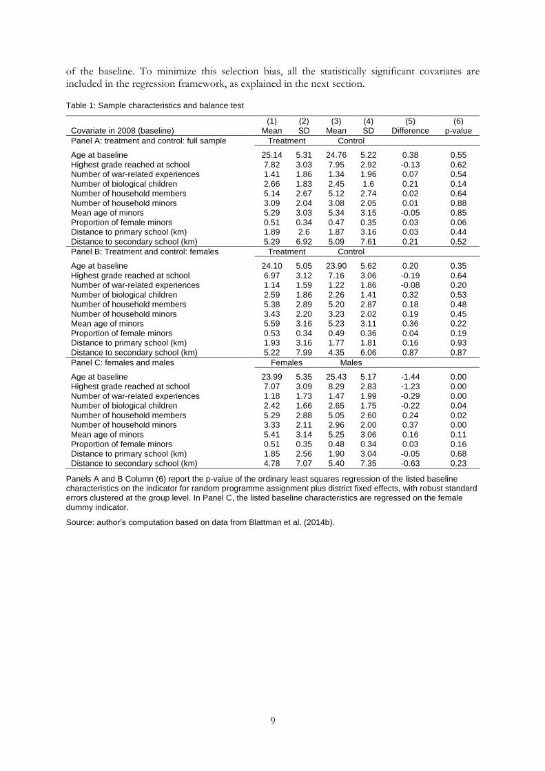
Table 1 presents descriptive statistics about the individual- and household-level pre-intervention characteristics of the sample.

Individuals are on average 25 years old, and they have an almost eighth-grade education, which corresponds to a completed primary education level. On average they have experienced at least one war-related event (most have witnessed violence). In spite of their young age, they already have a mean of 2.5 children. Households comprise about five members, with on average three minors—half of which are females. These minors are on average five years old in 2008, meaning that they are of school age at the time of the follow-ups. Indeed, minors represent the majority of household members, and almost every household (93 per cent) has at least one minor in its composition. The minors are mainly the biological children of the respondents, but the presence of other minors is also frequent (41 per cent of households include at least one). These other young family members are mostly nieces, nephews, or young siblings. Households are close enough to primary education facilities, with primary schools being generally not further than two kilometres away, whereas secondary schools are on average five kilometres away.

Table 1, Panel A, Column (6) shows the p-value of the balance test on the above-mentioned baseline covariates. Household characteristics seem to be well balanced, since none of the differences between treatment and control groups is significant at a 95 per cent level. Therefore the sample is also suitable for an analysis at household level. Panel B confirms that the women-only sample is well balanced too, while Panel C shows how men and women differed at the time

9 Blattman et al. (2014a) obtain this figure by dividing the group funds received by the estimated 2008 group size. Hence per-capita grant size varies across groups due to variations in group size and amounts requested.

9

of the baseline. To minimize this selection bias, all the statistically significant covariates are included in the regression framework, as explained in the next section.

Table 1: Sample characteristics and balance test

(1) (2) (3) (4) (5) (6) Covariate in 2008 (baseline) Mean SD Mean SD Difference p-value

Panel A: treatment and control: full sample Treatment Control

Age at baseline 25.14 5.31 24.76 5.22 0.38 0.55

Highest grade reached at school 7.82 3.03 7.95 2.92 -0.13 0.62 Number of war-related experiences 1.41 1.86 1.34 1.96 0.07 0.54

Number of biological children 2.66 1.83 2.45 1.6 0.21 0.14 Number of household members 5.14 2.67 5.12 2.74 0.02 0.64

Number of household minors 3.09 2.04 3.08 2.05 0.01 0.88 Mean age of minors 5.29 3.03 5.34 3.15 -0.05 0.85

Proportion of female minors 0.51 0.34 0.47 0.35 0.03 0.06 Distance to primary school (km) 1.89 2.6 1.87 3.16 0.03 0.44

Distance to secondary school (km) 5.29 6.92 5.09 7.61 0.21 0.52

Panel B: Treatment and control: females Treatment Control

Age at baseline 24.10 5.05 23.90 5.62 0.20 0.35

Highest grade reached at school 6.97 3.12 7.16 3.06 -0.19 0.64 Number of war-related experiences 1.14 1.59 1.22 1.86 -0.08 0.20

Number of biological children 2.59 1.86 2.26 1.41 0.32 0.53 Number of household members 5.38 2.89 5.20 2.87 0.18 0.48

Number of household minors 3.43 2.20 3.23 2.02 0.19 0.45 Mean age of minors 5.59 3.16 5.23 3.11 0.36 0.22

Proportion of female minors 0.53 0.34 0.49 0.36 0.04 0.19 Distance to primary school (km) 1.93 3.16 1.77 1.81 0.16 0.93

Distance to secondary school (km) 5.22 7.99 4.35 6.06 0.87 0.87

Panel C: females and males Females Males

Age at baseline 23.99 5.35 25.43 5.17 -1.44 0.00 Highest grade reached at school 7.07 3.09 8.29 2.83 -1.23 0.00

Number of war-related experiences 1.18 1.73 1.47 1.99 -0.29 0.00 Number of biological children 2.42 1.66 2.65 1.75 -0.22 0.04

Number of household members 5.29 2.88 5.05 2.60 0.24 0.02 Number of household minors 3.33 2.11 2.96 2.00 0.37 0.00

Mean age of minors 5.41 3.14 5.25 3.06 0.16 0.11 Proportion of female minors 0.51 0.35 0.48 0.34 0.03 0.16

Distance to primary school (km) 1.85 2.56 1.90 3.04 -0.05 0.68 Distance to secondary school (km) 4.78 7.07 5.40 7.35 -0.63 0.23

Panels A and B Column (6) report the p-value of the ordinary least squares regression of the listed baseline characteristics on the indicator for random programme assignment plus district fixed effects, with robust standard errors clustered at the group level. In Panel C, the listed baseline characteristics are regressed on the female dummy indicator.

Source: author’s computation based on data from Blattman et al. (2014b).

10

5 Methodology and results

5.1 Estimation method

My estimation is based on the following regression:

Yh POST = c + β Th + δ Xh + ϕ + εh POST [1]

where T is an indicator of assignment to treatment, X is a set of baseline covariates at the individual

and household level, ϕ represents district fixed effects, and standard errors are adjusted for

clustering at the group level. More specifically, X comprises a female dummy, age, education and human capital levels, initial level of capital and credit access, employment type and levels, and variables capturing group characteristics (as in Blattman et al. 2014a to ensure comparability).10 This set of covariates corrects for any baseline imbalance and guarantees similarity between the

treatment and control groups. The treatment effect is estimated by β, and the 2010 and 2012 impacts are evaluated separately. The survey weights are used, so the observations are weighted by their inverse probability of selection into the endline tracking.

My main outcomes of interest are household consumption and educational and health expenditures. Since I employ mostly household-aggregated measures instead of per-capita indicators, I also control for the number of household members, the number of household minors, and the number of biological children. Moreover, dealing with monetary variables, I cap all currency-denominated variables at the 99th percentile to avoid biases driven by extreme values. For comparability, I deflate all values to the 2008 correspondent.

For various reasons,11 out of the 265 treatment groups, 29 did not receive the grant. Thus regression [1] represents an intention-to-treat (ITT) estimation. To take into account imperfect compliance, I also employ instrumental variable estimations that use the initial assignment (ITT) as an instrument for actual treatment in order to assess the treatment effect on the treated (ToT). In showing the results I focus on the ITT estimates, while I present the ToT parameters as a robustness check.

Finally, since outcomes are self-reported, the treatment effect might be affected by over-reporting in the treatment group due to social desirability bias (i.e. the tendency to answer questions in a manner that can be viewed favourably) and under-reporting in the control group due to its desire to be included in future aid programmes. I try to overcome this issue by comparing the results for educational and health expenditures, which should be equally affected by social desirability bias,

10 The full list of variables included is: female (dummy); age (plus quadratic and cubic); located in a urban area (dummy); being unfound at baseline (dummy); risk aversion index; being enrolled in school (dummy); highest grade reached at school; distance in kilometres to educational facilities; able to read and write—even minimally (dummy); received prior vocational training (dummy); digit recall test score; index of physical disability; z-score of durable assets (z-score); savings in past six months; monthly gross cash earnings; can obtain 100,000 UGX loan (dummy); can obtain 1,000,000 UGX loan (dummy); average of weekly hours spent on: all non-agricultural work, casual low-skill labour, skilled trades, high-skill wage labour, other low-skill petty business, other non-agricultural work, household chores; zero employment hours in past month (dummy); main occupation is non-agricultural (dummy); engaged in a skilled trade (dummy); grant amount applied for in US$; group size; grant amount per member in US$; group existed before application (dummy); group age in years; z-score of within-group heterogeneity; z-score of quality of group dynamic; any leadership position in group (dummy); group chair or vice chair (dummy). All indicators refer to the baseline values.

11 See Blattman et al. (2014a) for an explanation.

11

and by also looking at household food and non-food consumption indicators, which are less likely to be significantly biased since they are based on aggregate computations from 135 different questions.

5.2 Impacts on household expenditures

Impacts on consumption

Table 2: Intent-to-treat estimates of programme impact on household consumption

(1) (2) (3) (4) (5) (6) (7)

HH consump-tion per capita

HH consump-

tion

Ln(HH consump-

tion)

HH food consump-

tion

Ln(HH food

consump-tion)

HH non-food

consump-tion

Ln(HH non-food consump-

tion)

2012 2012 2012 2012 2012 2012 2012

Full sample ITT 3.5** 23.17*** 0.072*** 14.66*** 0.057*** 8.4*** 0.047***

SE (1.414) (6.983) (0.02) (4.961) (0.017) (3.11) (0.015)

Control mean 29.33 199.75 5.61 149.74 5.45 47.77 4.94

Male ITT 3.21* 22.42*** 0.071*** 12.77** 0.052** 9.25*** 0.053***

SE (1.837) (8.657) (0.024) (6.186) (0.021) (3.548) (0.018)

Control mean 30.53 204.97 5.63 156.29 5.48 46.19 4.93

Female ITT 4.04** 24.57** 0.074** 18.16** 0.066** 6.82 0.036

SE (1.79) (11.23) (0.031) (7.799) (0.027) (5.432) (0.026)

Control mean 27.2 190.48 5.58 138.11 5.41 50.56 4.96

Female - male ITT 0.83 2.15 0.004 5.39 0.014 -2.43 -0.018

SE (2.405) (13.92) (0.038) (9.73) (0.032) (6.228) (0.03)

Observations 1,866 1,866 1,866 1,866 1,866 1,865 1,865

R-squared 0.142 0.240 0.251 0.211 0.211 0.196 0.225

Columns (1) to (7) report the ITT estimates of programme impact for the full sample, males only, and females only. Robust standard errors are in brackets, clustered by group. The mean level of the dependent variable in the control group is reported below the standard error. Each ITT is calculated via a weighted least squares regression of the dependent variable on the programme assignment indicator, district fixed effects, and a vector of control variables listed in the text and described in Blattman et al. (2014a). The models from (2) to (7) also include the number of household members as a control. As in Blattman et al. (2014a), the male- and female-only ITTs are calculated in a pooled regression (within each endline round) that includes an interaction between programme assignment and the female dummy; thus the female ITT is the sum of the coefficients on programme assignment and this interaction. All consumption variables were top-censored at the 99th percentile to contain outliers and deflated to 2008 values. Columns (1), (2), (4), and (6) report values in 000s of UGX. *** p<0.01, ** p<0.05, * p<0.1.


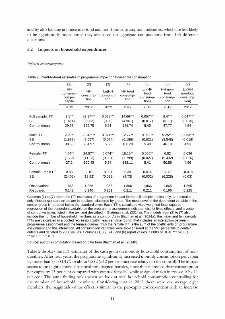
Table 2 displays the ITT estimates of the cash grant on monthly household consumption of non-durables. After four years, the programme significantly increased monthly consumption per capita by more than 3,000 UGX or about US$2 (a 12 per cent increase relative to the control). The impact seems to be slightly more substantial for assigned females, since they increased their consumption per capita by 15 per cent compared with control females, while assigned males increased it by 11 per cent. The same finding holds when we look at total household consumption controlling for the number of household members. Considering that in 2012 there were on average eight members, the magnitude of the effect is similar to the per-capita correspondent with an increase

12

of US$13 or again 12 per cent. The result is also confirmed when we use the log variable in place of the level indicator.

Food consumption in the treatment group rose significantly by 10 per cent (14,660 UGX or about US$8), and non-food consumption grew relevantly by 18 per cent (8,400 UGX or US$5). The decomposition in food and non-food expenditures shows interesting gender differences. While women assigned to receive the grant spent about US$10 more on food consumption, they only spent US$3–4 more on non-food consumption. On the other hand, men in the treatment group increased food consumption by 8 per cent and non-food consumption by 20 per cent relative to men in the control group. This spending preference of males could be either positive or negative for household welfare, depending on the types of non-food expenses privileged.

Impacts on educational and health expenditures

Table 3: Intent-to-treat estimates of programme impact on household educational and health expenditures

(1) (2) (3) (4) (5) (6) (7) (8)

Total educational

expenditures Ln(Total educational

expenditures) Total health expenditures

Ln(Total health expenditures)

2010 2012 2010 2012 2010 2012 2010 2012

Full sample ITT 40.11 28.8 0.067* 0.077* 6.79** 0.26 0.038*** 0.008

SE (28.72) (21.67) (0.04) (0.042) (2.725) (2.792) (0.014) (0.014)

Control mean 272.06 250.63 5.4 5.41 29.14 29.61 4.82 4.8

Male ITT 56.51 54.78** 0.121** 0.122** 7.65** -0.11 0.043** 0.004

SE (36.06) (24.52) (0.05) (0.048) (3.472) (3.445) (0.018) (0.017)

Control mean 270.6 225.47 5.39 5.37 29.82 31.34 4.82 4.81

Female ITT 8.49 -19.58 -0.037 -0.006 5.14 0.94 0.028 0.016

SE (42.38) (38.56) (0.063) (0.07) (3.626) (4.878) (0.02) (0.023)

Control mean 274.72 295.31 5.42 5.49 27.91 26.54 4.81 4.79

Female - male ITT -48.02 -74.36* -0.158** -0.128 -2.518 1.045 -0.014 0.012

SE (53.52) (43.89) (0.078) (0.08) (4.718) (6.022) (0.026) (0.028)

Observations 2,000 1,860 2,000 1,860 2,000 1,860 2,000 1,860

R-squared 0.159 0.214 0.249 0.252 0.109 0.133 0.121 0.122

Columns (1) to (8) report the ITT estimates of programme impact for the full sample, males only, and females only. Robust standard errors are in brackets, clustered by group. The mean level of the dependent variable in the control group is reported below the standard error. Each ITT is calculated via a weighted least squares regression of the dependent variable on: the programme assignment indicator, the number of household members, the number of household minors, the number of biological children, district fixed effects, and a vector of control variables listed in the text and described in Blattman et al. (2014a). As in that article, the male- and female-only ITTs are calculated in a pooled regression (within each endline round) that includes an interaction between programme assignment and the female dummy; thus the female ITT is the sum of the coefficients on programme assignment and this interaction. All consumption variables were top-censored at the 99th percentile to contain outliers and deflated to 2008 values. Columns (1), (2), (5), and (6) report values in 000s of UGX. *** p<0.01, ** p<0.05, * p<0.1.


13

I focus on total expenditures on education and health made in the 12 months before the survey. In Table 3, I consider household-aggregated measures12 while controlling for the number of household members, the number of household minors, and the number of biological children.

The programme impact on educational expenditures is statistically significant only in logs, but corresponds to a quite substantial relative increase of 11–15 per cent (29,000–40,000 UGX or US$17–23) in 2010 and 2012 (Table 3). The intervention also caused a significant growth in shorter-term health expenditures by 23 per cent (about 7,000 UGX or US$4), but the effect is close to zero after four years. The results are confirmed by the illustration of the relative log distributions (Figure 2).13

Figure 2: Kernel densities of educational and health expenditures

(a) Educational expenditures in 2010 (left) and 2012 (right)

(b) Health expenditures in 2010 (left) and 2012 (right)


Passing on to the gender-differentiated impacts, in 2010 males assigned to receive the grant increased total educational expenditures by 21 per cent (the effect is significant when we look at the log results). In 2012 their educational expenditures increased even more, by a statistically significant 24 per cent, whereas educational expenditures of females in the treatment group decreased. On the other hand, there is no significant gender heterogeneity in health expenditures.

12 The results do not depend on this choice, however.

13 In 2012 the kernel density of educational expenditures in the treatment group is more pronouncedly above the control group than it was in 2010. The reverse is true in the case of health expenses. In the shorter run, the cash grant decreased the proportion of households not (or almost not) spending on health, while the effect dissipated in 2012.

14

In economic terms, among males in the treatment group, educational expenditures increased by US$32 in both the short and long run, and health expenditures increased only temporarily by about US$5.

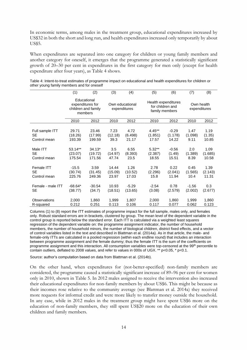
When expenditures are separated into one category for children or young family members and another category for oneself, it emerges that the programme generated a statistically significant growth of 20–30 per cent in expenditures in the first category for men only (except for health expenditure after four years), as Table 4 shows.

Table 4: Intent-to-treat estimates of programme impact on educational and health expenditures for children or other young family members and for oneself

(1) (2) (3) (4) (5) (6) (7) (8)

Educational expenditures for

children and family members

Own educational expenditures

Health expenditures for children and family members

Own health expenditures

2010 2012 2010 2012 2010 2012 2010 2012

Full sample ITT 29.71 23.46 7.23 4.72 4.45** -0.29 1.47 1.19

SE (18.26) (17.99) (12.18) (6.498) (1.851) (1.178) (1.098) (1.35)

Control mean 193.39 199.59 39.3 21.17 17.57 14.22 9.11 10.85

Male ITT 53.14** 34.13* 3.5 6.55 5.32** -0.56 2.0 1.09

SE (23.07) (19.72) (14.97) (8.393) (2.387) (1.49) (1.389) (1.685)

Control mean 175.54 171.56 47.74 23.5 18.55 15.51 8.39 10.58

Female ITT -15.5 3.59 14.44 1.26 2.78 0.22 0.45 1.39

SE (30.74) (31.45) (15.09) (10.52) (2.296) (2.041) (1.565) (2.143)

Control mean 225.76 249.36 23.97 17.03 15.8 11.94 10.4 11.31

Female - male ITT -68.64* -30.54 10.93 -5.29 -2.54 0.78 -1.56 0.3

SE (38.77) (34.7) (18.51) (13.65) (3.08) (2.579) (2.002) (2.677)

Observations 2,000 1,860 1,999 1,807 2,000 1,860 1,999 1,860

R-squared 0.212 0.251 0.113 0.106 0.117 0.077 0.062 0.123

Columns (1) to (8) report the ITT estimates of programme impact for the full sample, males only, and females only. Robust standard errors are in brackets, clustered by group. The mean level of the dependent variable in the control group is reported below the standard error. Each ITT is calculated via a weighted least squares regression of the dependent variable on: the programme assignment indicator, the number of household members, the number of household minors, the number of biological children, district fixed effects, and a vector of control variables listed in the text and described in Blattman et al. (2014a). As in that article, the male- and female-only ITTs are calculated in a pooled regression (within each endline round) that includes an interaction between programme assignment and the female dummy; thus the female ITT is the sum of the coefficients on programme assignment and this interaction. All consumption variables were top-censored at the 99th percentile to contain outliers, deflated to 2008 values, and refer to values in 000s of UGX. ** p<0.05, * p<0.1.


On the other hand, when expenditures for (not-better-specified) non-family members are considered, the programme caused a statistically significant increase of 89–96 per cent for women only in 2010, shown in Table 5. In 2012 males assigned to receive the intervention also increased their educational expenditures for non-family members by about US$6. This might be because as their incomes rose relative to the community average (see Blattman et al. 2014a) they received more requests for informal credit and were more likely to transfer money outside the household. In any case, while in 2012 males in the treatment group might have spent US$6 more on the education of non-family members, they still spent US$20 more on the education of their own children and family members.

15

Table 5: Intent-to-treat estimates of programme impact on educational and health expenditures for non-family members

(1) (2) (3) (4)

Educational expenditures for non-family members

Health expenditures for non-family members

2010 2012 2010 2012

Full sample ITT 5.14 4.7 0.47 0.51*

SE (3.7) (4.258) (0.292) (0.27)

Control mean 18.05 17.54 1.35 1.34

Male ITT 3.28 10.63** 0.27 0.43

SE (4.809) (5.032) (0.363) (0.335)

Control mean 22.57 18.5 1.6 1.53

Female ITT 8.74* -6.34 0.86* 0.66

SE (4.61) (6.983) (0.466) (0.497)

Control mean 9.84 15.83 0.9 0.99

Female - male ITT 5.46 -16.97** 0.59 0.23

SE (6.244) (8.235) (0.58) (0.622)

Observations 1,999 1,860 2,000 1,860

R-squared 0.071 0.084 0.043 0.071

Columns (1) to (4) report the ITT estimates of programme impact for the full sample, males only, and females only. Robust standard errors are in brackets, clustered by group. The mean level of the dependent variable in the control group is reported below the standard error. Each ITT is calculated via a weighted least squares regression of the dependent variable on: the programme assignment indicator, the number of household members, the number of household minors, the number of biological children, district fixed effects, and a vector of control variables listed in the text and described in Blattman et al. (2014a). As in that article, the male- and female-only ITTs are calculated in a pooled regression (within each endline round) that includes an interaction between programme assignment and the female dummy; thus the female ITT is the sum of the coefficients on programme assignment and this interaction. All consumption variables were top-censored at the 99th percentile to contain outliers, deflated to 2008 values, and refer to values in 000s of UGX. ** p<0.05, * p<0.1.


These findings suggest that females were more affected by requests from external individuals, especially shortly after receiving the grant. Rather than gender differences in spending, this result might reflect poor female decision-making power. The treatment effects on household consumption suggest that females who were assigned to receive the grant tried to provide more for their families in those aspects that were under their control, such as everyday food expenses. However, they did not manage to make more substantial investments in the education of their children. I hypothesize this is due at least in part to stronger redistributive pressures exerted on women.

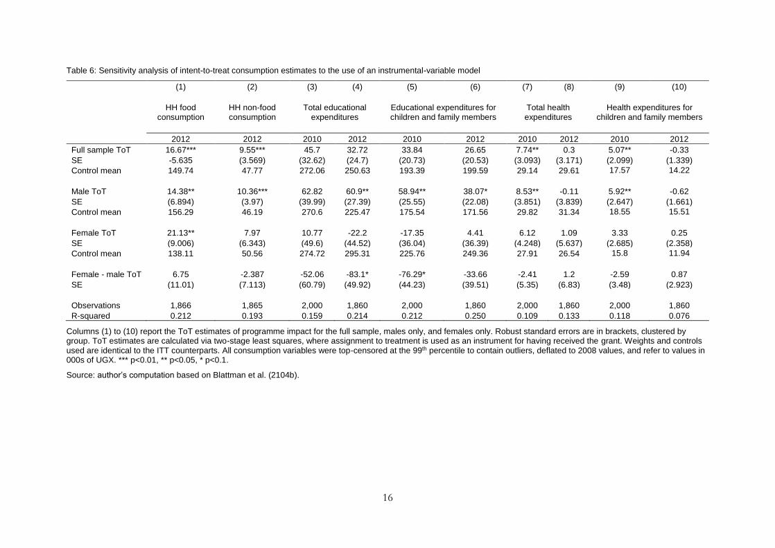
Finally, Table 6 reproduces the treatment impact using the ToT estimations. As expected, the results are similar to the ITT estimates, with the only difference that the magnitudes of the effects are about two per cent higher, since they now refer to those that did indeed receive the money.

16

Table 6: Sensitivity analysis of intent-to-treat consumption estimates to the use of an instrumental-variable model

(1) (2) (3) (4) (5) (6) (7) (8) (9) (10)

HH food consumption

HH non-food consumption

Total educational expenditures

Educational expenditures for children and family members

Total health expenditures


2012 2012 2010 2012 2010 2012 2010 2012 2010 2012

Full sample ToT 16.67*** 9.55*** 45.7 32.72 33.84 26.65 7.74** 0.3 5.07** -0.33

SE -5.635 (3.569) (32.62) (24.7) (20.73) (20.53) (3.093) (3.171) (2.099) (1.339)

Control mean 149.74 47.77 272.06 250.63 193.39 199.59 29.14 29.61 17.57 14.22

Male ToT 14.38** 10.36*** 62.82 60.9** 58.94** 38.07* 8.53** -0.11 5.92** -0.62

SE (6.894) (3.97) (39.99) (27.39) (25.55) (22.08) (3.851) (3.839) (2.647) (1.661)

Control mean 156.29 46.19 270.6 225.47 175.54 171.56 29.82 31.34 18.55 15.51

Female ToT 21.13** 7.97 10.77 -22.2 -17.35 4.41 6.12 1.09 3.33 0.25

SE (9.006) (6.343) (49.6) (44.52) (36.04) (36.39) (4.248) (5.637) (2.685) (2.358)

Control mean 138.11 50.56 274.72 295.31 225.76 249.36 27.91 26.54 15.8 11.94

Female - male ToT 6.75 -2.387 -52.06 -83.1* -76.29* -33.66 -2.41 1.2 -2.59 0.87

SE (11.01) (7.113) (60.79) (49.92) (44.23) (39.51) (5.35) (6.83) (3.48) (2.923)

Observations 1,866 1,865 2,000 1,860 2,000 1,860 2,000 1,860 2,000 1,860

R-squared 0.212 0.193 0.159 0.214 0.212 0.250 0.109 0.133 0.118 0.076

Columns (1) to (10) report the ToT estimates of programme impact for the full sample, males only, and females only. Robust standard errors are in brackets, clustered by group. ToT estimates are calculated via two-stage least squares, where assignment to treatment is used as an instrument for having received the grant. Weights and controls used are identical to the ITT counterparts. All consumption variables were top-censored at the 99th percentile to contain outliers, deflated to 2008 values, and refer to values in 000s of UGX. *** p<0.01, ** p<0.05, * p<0.1.

Source: author’s computation based on Blattman et al. (2104b).

17

Impacts on other types of expenditures for children

To check whether my findings are consistent with the results on other expenditure dimensions, I look in more detail at the consumption module of the final endline survey and assess the treatment impacts on expenditures on clothes, shoes, and other material for adults versus minors (separated into males and females), expenditures on educational materials (i.e. books, stationery, and school uniforms), and expenditures on medical treatments and medicines. Table 7 offers a picture that confirms previous results.

Table 7: Intent-to-treat estimates of programme impact on other types of household expenditures

(1) (2) (3) (4) (5) (6)

Clothes/ shoes

expenditures for males

over 16

Clothes/ shoes

expenditures for

females over 16

Clothes/ shoes

expenditures for male

minors under 16

Clothes/ shoes

expenditures for female

minors under 16

Expenditures for

educational material

Expenditures for medical treatments

and medicines

2012 2012 2012 2012 2012 2012

Full sample ITT 7.97*** 7.07*** 2.86* 1.69 8.24** 6.38

SE (2.497) (2.391) (1.534) (1.421) (3.449) (4.717)

Control mean 34.69 34.27 25.87 24.45 48.37 63.02

Male ITT 7.11** 6.07** 3.77* 1.16 9.94** 2.57

SE (3.224) (3.053) (1.996) (1.589) (4.179) (6.012)

Control mean 38.82 37.4 26.24 24.75 45.79 65.0

Female ITT 9.58** 8.93** 1.16 2.67 5.07 13.49*

SE (4.155) (3.672) (2.295) (2.739) (5.858) (7.372)

Control mean 27.19 28.67 25.19 23.9 52.99 59.46

Female - male ITT 2.48 2.86 -2.61 1.52 -4.88 10.92

SE (5.375) (4.722) (3.029) (3.141) (7.097) (9.434)

Observations 1,848 1,853 1,850 1,851 1,855 1,852

R-squared 0.106 0.119 0.137 0.119 0.177 0.072

Columns (1) to (6) report the ITT estimates of programme impact for the full sample, males only, and females only. Robust standard errors are in brackets, clustered by group. The mean level of the dependent variable in the control group is reported below the standard error. Each ITT is calculated via a weighted least squares regression of the dependent variable on: the programme assignment indicator, the number of household members, the number of household minors, the number of biological children, district fixed effects, and a vector of control variables listed in the text and described in Blattman et al. (2014a). As in that article, the male- and female-only ITTs are calculated in a pooled regression (within each endline round) that includes an interaction between programme assignment and the female dummy; thus the female ITT is the sum of the coefficients on programme assignment and this interaction. All consumption variables were top-censored at the 99th percentile to contain outliers, deflated to 2008 values, and refer to values in 000s of UGX. *** p<0.01, ** p<0.05, * p<0.1.


On the one hand, males assigned to treatment increased their expenditures on clothes and shoes for adults by 16–18 per cent, and also increased expenditures on clothes and shoes for male minors by 14 per cent (the five per cent increase for female minors is not significant). At the same time, their expenditures on educational material grew by 22 per cent, whereas their medical expenditures rose by merely four per cent. On the other hand, assigned females increased their expenditures on adults’ clothes and shoes by 31–35 per cent, but they did not substantially increase expenditures

18

for minors.14 At the same time, their medical expenses relevantly increased by 23 per cent, while their expenditures on educational materials increased by only 10 per cent. This suggests that males assigned to receive the grant consumed more with regard to education-related items, and provided for adults as well as for minors, especially males. Females, on the other hand, apparently spent more on (were in better charge of) food consumption and health-related expenses.

5.3 Heterogeneous impacts

To test for heterogeneity in the treatment effect based on observable characteristics, I run the following set of regressions:

Yh POST = c + β Th + γ Th x TRAITh + η TRAITh +δ Xh + ϕ + εh POST [2]

where TRAIT is the vector of background characteristics along which theory would predict heterogeneity in the programme impacts. The effect of the intervention for the subgroup of people

with a given trait is given by the sum of the coefficients β and γ; if γ is significantly different from zero, then there is evidence of heterogeneity in the treatment effect for that trait. As an outcome variable I focus only on educational expenditures, since they offer more useful insights into the differentiated effects of the programme.

In particular, I estimate equation [2] for the following baseline characteristics: wealth, having witnessed violence at baseline, number of foster children in the household, proportion of female household minors, and mean age of household minors. Table 8 illustrates the heterogeneous results for the whole sample. Individuals in the treatment group with higher baseline wealth and with more foster children in the household had higher total educational expenditures (by about US$35 and US$44 respectively after four years, whereas the effect for the full sample was of only US$17). While the effect of foster children is as expected, the magnifying role of wealth signals that the grant did not necessarily work as an anti-poverty intervention, as it did not strongly support investments by the poorest. Interestingly, people that had witnessed violence also raised their educational expenditures (by about US$30). This might be due to a difference in social preferences, since it has been shown that individuals exposed to violence display more altruistic behaviours (Voors et al. 2012). Their higher altruism might explain why they seem to have spent more on non-family members and less on themselves. Surprisingly, there is no heterogeneity based on the proportion of female minors in the household, whereas the treatment impact is heterogeneous based on the average age of the minors. The effect of age is unclear, however: it is negative in 2010 and positive in 2012.

In order to explore which constraints influenced the educational expenditures of females, I also estimate equation [2] for the smaller sample of female respondents. I identified the following baseline characteristics that might be especially relevant for women: baseline education, being married, number of groups one belongs to, dissatisfaction with the YOP group, and the standard deviation of human capital within the YOP group.

14 The treatment effect is positive, equal to an 11 per cent increase for clothes and shoes for females and a five per cent increase for clothes and shoes for males, but it is not statistically significant.

19

Table 8: Heterogeneity of programme impact on educational expenditures

(1) (2) (3) (4) (5) (6) (7) (8)






non-family members

2010 2012 2010 2012 2010 2012 2010 2012

Panel 1: heterogeneity for baseline wealth Assigned to treatment (ITT) 24.34 20.42 22.85 11.96 3.23 2.93 1.74 6.13

SE (25.72) (19.61) (17.58

) (15.87) (8.91) (5.68) (3.2) (3.81)

ITT x wealth index 37.28 40.98** 27.44 22.19 6.46 7.61 -2.49 4.02

SE (25.04) (19.17) (17.12

) (15.51) (8.67) (5.53) (3.11) (3.72) Observations 2,000 1,860 2,000 1,860 1,999 1,807 1,999 1,860

R-squared 0.153 0.207 0.198 0.236 0.108 0.093 0.071 0.078

Panel 2: heterogeneity for having witnessed violence at baseline

Assigned to treatment (ITT) 17.61 -0.06 7.93 -0.43 13.63 1.39 2.42 1.72

SE (28.08) (21.38) (19.18

) (17.30) (9.7) (6.19) (3.49) (4.15)

ITT x violence witnessed 9.24 52.0* 43.62 32.74 -

41.06*** 1.58 -1.5 13.48**

SE (42.69) (31.47) (29.16

) (25.46) (14.75) (9.09) (5.3) (6.1) Observations 2,000 1,860 2,000 1,860 1,999 1,807 1,999 1,860 R-squared 0.152 0.206 0.198 0.236 0.111 0.092 0.071 0.081

Panel 3: heterogeneity for number of foster minors in the household

Assigned to treatment (ITT) 2.91 -8.98 12.52 -4.1 0.48 1.25 -0.56 0.25

SE (26.96) (20.55) (18.42

) (16.65) (9.29) (5.98) (3.36) (3.95)

ITT x no. foster minors 64.83*

* 85.67**

* 27.76 47.13*

* 9.66 0.5 8.2** 19.81**

*

SE (28.83) (22.64) (19.70

) (18.35) (9.93) (6.63) (3.59) (4.35) Observations 1,966 1,828 1,966 1,828 1,965 1,775 1,965 1,828

R-squared 0.154 0.212 0.199 0.239 0.108 0.093 0.074 0.092

Panel 4: heterogeneity for proportion of female minors in the household

Assigned to treatment (ITT) 35.04 28.65 27.36 30.36 9.02 -2.59 -7.18 3.81

SE (52.89) (41.24) (37.44

) (34.38) (15.71) (9.76) (6.85) (7.52) ITT x prop. female minors 4.51 -35.76 17.73 -29.55 -21.12 8.07 14.34 -7.81

SE (86.79) (67.47) (61.43

) (56.25) (25.79) (15.96

) (11.24

) (12.3) Observations 1,338 1,257 1,338 1,257 1,337 1,224 1,337 1,257 R-squared 0.166 0.219 0.211 0.242 0.092 0.065 0.098 0.093

Panel 5: heterogeneity for mean age of minors in the household

Assigned to treatment (ITT) -42.14 53.67 -31.72 77.28* 6.69 0.41 -4.46 -10.29

SE (61.54) (47.3) (43.56

) (39.43) (18.05) (11.21

) (8.07) (8.6)

ITT x minors’ mean age 15.88 -8.82 13.57* -12.49* -1.69 0.25 0.92 2.0 SE (10.17) (7.71) (7.2) (6.43) (2.98) (1.82) (1.33) (1.4) Observations 1,350 1,272 1,350 1,272 1,349 1,239 1,349 1,272

R-squared 0.178 0.222 0.223 0.243 0.089 0.068 0.097 0.095

Columns (1) to (8) report coefficients from a weighted least squares regression of the dependent variable on the listed interaction and independent variables, the number of household members, the number of household minors, the number of biological children, district fixed effects, and a vector of control variables listed in the text

20

and described in Blattman et al. (2014a). Robust standard errors are in brackets, clustered by group. All consumption variables were top-censored at the 99th percentile to contain outliers, deflated to 2008 values, and refer to values in 000s of UGX. *** p<0.01, ** p<0.05, * p<0.1.


Table 9: Heterogeneity of programme impact on educational expenditures for females

(1) (2) (3) (4) (5) (6) (7) (8)






non-family members

2010 2012 2010 2012 2010 2012 2010 2012

Panel 1: heterogeneity for baseline education (at least secondary)

Assigned to treatment (ITT) -51.88 -31.04 -59.78* -20.04 2.85 -1.93 5.38 -0.88 SE (46.38) (41.79) (33.86) (35.79) (13.42) (9.0) (5.59) (6.76)

ITT x education 174.6 10.73 176.8** 31.03 10.79 -14.34 14.93 -1.52 SE (107.6) (99.6) (78.55) (85.29) (31.12) (21.08) (12.97) (16.12) Observations 667 627 667 627 666 607 666 627

R-squared 0.273 0.247 0.302 0.276 0.186 0.168 0.124 0.110

Panel 2: heterogeneity for being married

Assigned to treatment (ITT) -40.66 -49.7 -55.94 -38.07 13.0 -7.51 7.55 0.95

SE (57.83) (51.25) (42.14) (43.96) (16.7) (11.08) (6.94) (8.28) ITT x married 52.44 44.33 67.62 50.44 -15.55 7.12 0.62 -4.91

SE (81.7) (73.7) (59.52) (63.2) (23.61) (15.91) (9.81) (11.9) Observations 666 626 666 626 665 606 665 626 R-squared 0.263 0.250 0.290 0.276 0.182 0.162 0.127 0.117

Panel 3: heterogeneity for number of groups one belongs to

Assigned to treatment (ITT) -211.5** 1.54 -174.3*** 7.08 1.52 -6.11 4.8 -1.91 SE (84.46) (73.51) (61.78) (63.1) (24.48) (15.83) (10.2) (11.9)

ITT x no. groups 103.0*** -17.57 78.83*** -12.42 1.99 0.88 1.79 0.15 SE (39.13) (32.91) (28.63) (28.25) (11.34) (7.13) (4.72) (5.33) Observations 667 627 667 627 666 607 666 627

R-squared 0.273 0.255 0.299 0.279 0.181 0.162 0.120 0.117

Panel 4: heterogeneity for dissatisfaction with YOP group

Assigned to treatment (ITT) -18.68 -30.45 -26.35 -15.77 6.71 -4.25 7.86 -2.04

SE (42.9) (38.63) (31.37) (33.07) (12.33) (8.23) (5.14) (6.21) ITT x dissatisfaction YOP 9.35 31.54 5.13 27.18 -13.75 -11.06 1.71 17.55**


21

Panel 5: heterogeneity for standard deviation of human capital within YOP group

Assigned to treatment (ITT) 21.57 97.26 -10.03 25.81 43.23 32.05* -17.35 0.42

SE (97.97) (88.64) (71.61) (75.95) (28.19) (18.98) (11.77) (14.32) ITT x SD human capital YOP -64.44 -253.5 -23.65 -79.09 -72.11 -72.44** 51.25** -4.43


Columns (1) to (8) report coefficients from a weighted least squares regression of the dependent variable on the listed interaction and independent variables, the number of household members, the number of household minors, the number of biological children, district fixed effects, and a vector of control variables listed in the text and described in Blattman et al. (2014a). Robust standard errors are in brackets, clustered by group. All consumption variables were top-censored at the 99th percentile to contain outliers, deflated to 2008 values, and refer to values in 000s of UGX. *** p<0.01, ** p<0.05,* p<0.1.


Table 9 shows the relative heterogeneous effects of the programme on females. Better-educated females (who had completed at least secondary school) assigned to receive the grant spent significantly more on education, especially in the shorter run and for their children and family members (in 2010 they spent about US$68 more for them). Being married does not seem to affect their educational expenditures, while belonging to more groups is detrimental. Females that were assigned to receive the grant and belonged to more groups spent US$55 less in 2010 for their children and family members, and US$62 less in total. Similarly, the results suggest that women that were dissatisfied with their YOP group suffered stronger redistributive pressures and spent significantly more on non-family members (US$6 after two years—versus US$4 for the full female sample—and US$9 after four years). In particular, it seems that women belonging to YOP groups with higher human capital heterogeneity (higher standard deviation) were substantially more affected by external requests. In 2010 they spent about US$20 more on educational expenditures for non-family members, while they spent significantly less on their own educational expenditures.

5.4 Impacts on educational outcomes

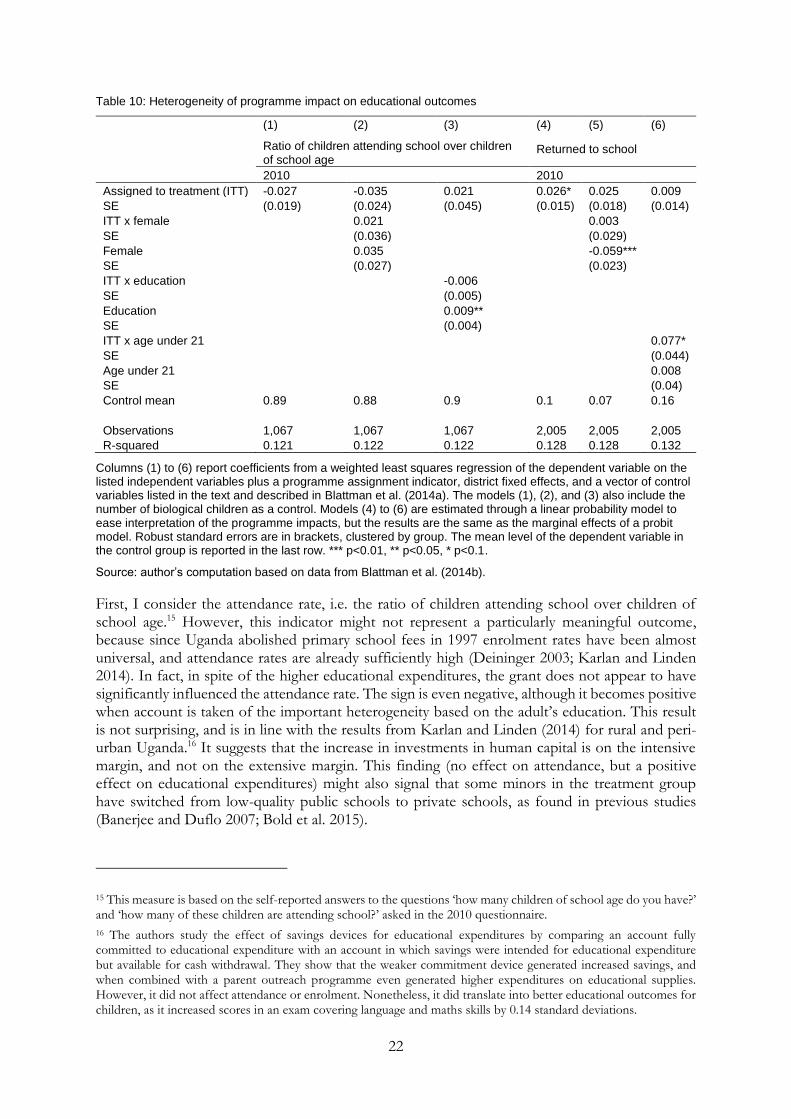
Did the increase in educational expenditures also translate into better educational outcomes for children and adolescents in Northern Uganda? The evaluation of the YOP intervention and the related questionnaires were not specifically designed to reply to this question, and given the lack of suitable outcome indicators it is not possible to give a clear answer. Table 10, showing the results on the only two education-related outcome measures available in the data set, suggests that the response might be yes.

22

Table 10: Heterogeneity of programme impact on educational outcomes

(1) (2) (3) (4) (5) (6)

Ratio of children attending school over children of school age

Returned to school

2010 2010

Assigned to treatment (ITT) -0.027 -0.035 0.021 0.026* 0.025 0.009

SE (0.019) (0.024) (0.045) (0.015) (0.018) (0.014)

ITT x female 0.021 0.003

SE (0.036) (0.029)

Female 0.035 -0.059***

SE (0.027) (0.023)

ITT x education -0.006

SE (0.005)

Education 0.009**

SE (0.004)

ITT x age under 21 0.077*

SE (0.044)

Age under 21 0.008

SE (0.04)

Control mean 0.89 0.88 0.9 0.1 0.07 0.16

Observations 1,067 1,067 1,067 2,005 2,005 2,005

R-squared 0.121 0.122 0.122 0.128 0.128 0.132

Columns (1) to (6) report coefficients from a weighted least squares regression of the dependent variable on the listed independent variables plus a programme assignment indicator, district fixed effects, and a vector of control variables listed in the text and described in Blattman et al. (2014a). The models (1), (2), and (3) also include the number of biological children as a control. Models (4) to (6) are estimated through a linear probability model to ease interpretation of the programme impacts, but the results are the same as the marginal effects of a probit model. Robust standard errors are in brackets, clustered by group. The mean level of the dependent variable in the control group is reported in the last row. *** p<0.01, ** p<0.05, * p<0.1.


First, I consider the attendance rate, i.e. the ratio of children attending school over children of school age.15 However, this indicator might not represent a particularly meaningful outcome, because since Uganda abolished primary school fees in 1997 enrolment rates have been almost universal, and attendance rates are already sufficiently high (Deininger 2003; Karlan and Linden 2014). In fact, in spite of the higher educational expenditures, the grant does not appear to have significantly influenced the attendance rate. The sign is even negative, although it becomes positive when account is taken of the important heterogeneity based on the adult’s education. This result is not surprising, and is in line with the results from Karlan and Linden (2014) for rural and peri-urban Uganda.16 It suggests that the increase in investments in human capital is on the intensive margin, and not on the extensive margin. This finding (no effect on attendance, but a positive effect on educational expenditures) might also signal that some minors in the treatment group have switched from low-quality public schools to private schools, as found in previous studies (Banerjee and Duflo 2007; Bold et al. 2015).

15 This measure is based on the self-reported answers to the questions ‘how many children of school age do you have?’ and ‘how many of these children are attending school?’ asked in the 2010 questionnaire.

16 The authors study the effect of savings devices for educational expenditures by comparing an account fully committed to educational expenditure with an account in which savings were intended for educational expenditure but available for cash withdrawal. They show that the weaker commitment device generated increased savings, and when combined with a parent outreach programme even generated higher expenditures on educational supplies. However, it did not affect attendance or enrolment. Nonetheless, it did translate into better educational outcomes for children, as it increased scores in an exam covering language and maths skills by 0.14 standard deviations.

23

Second, I look at the probability of returning to school. This indicator is complementary to the analysis of educational expenditures and outcomes for children, since it is mostly related to one’s own educational expenses, and it refers more appropriately to younger grant recipients, who do not represent the majority of parents. Nevertheless, it offers interesting insights into the education-related impact of the programme. In 2010 individuals assigned to receive the grant were 26 per cent more likely to have returned to school relative to their control counterparts. The intervention was even more effective among the younger cohorts, since there is significant heterogeneity based on age. In 2010 individuals in the treatment group that had been under 21 in 2008 were 54 per cent more likely to have returned to school.

Finally, I shed more light on the educational effects of the grant by exploring self-assessed outcomes related to education and access to basic services (Table 11). Using a nine-step ladder with the least educated children in the class standing on the lowest rung and the most educated on the highest, parents in the treatment group placed their children six per cent higher than the control group—while assigned males placed their children eight per cent higher than control males. Similarly, referring to a one-to-nine scale with those in the community who have the least access to basic services (such as health and education) at the bottom, individuals assigned to receive the grant placed their families 11 per cent higher relative to the control. On the other hand, there appears to be no effect on self-assessed child health. These findings suggest that the intervention increased not only educational expenditures, but also subjective education-related outcomes.

Table 11: Intent-to-treat estimates of programme impact on self-assessed educational and health measures

(1) (2) (3)

Self-assessed child education, on a scale from 1 to 9

Self-assessed child health, on a scale from 1 to 9

Self-assessed access to basic services such as education and health, on a scale from 1 to 9

2010 2010 2010

Full sample ITT 0.21** 0.13 0.41***

SE (0.107) (0.107) (0.097)

Control mean 3.47 4.78 3.68

Male ITT 0.29** 0.15 0.42***

SE (0.129) (0.127) (0.115)


Female ITT 0.07 0.08 0.38**

SE (0.171) (0.188) (0.17)


Female - male ITT -0.22 -0.07 -0.04

SE (0.206) (0.224) (0.202)

Observations 1,728 1,783 1,983

R-squared 0.119 0.087 0.101

Columns (1) to (3) report the ITT estimates of programme impact for the full sample, males only, and females only. Robust standard errors are in brackets, clustered by group. The mean level of the dependent variable in the control group is reported below the standard error. Each ITT is calculated via a weighted least squares regression of the dependent variable on a programme assignment indicator, district fixed effects, and a vector of control variables listed in the text and described in Blattman et al. (2014a). As in that article, the male- and female-only ITTs are calculated in a pooled regression (within each endline round) that includes an interaction between programme assignment and the female dummy; thus the female ITT is the sum of the coefficients on programme assignment and this interaction. *** p<0.01, ** p<0.05.


24

6 Discussion and conclusion

On average, the YOP programme had a positive effect on education-related expenditures. This suggests that the intervention supported investments not only in productive assets, but also in human capital. Different reasons might explain such an effect.

Educational expenditures might be an expenditure item that people can afford only when released from credit constraints. Otherwise, it might be that the connection with a community facilitator (generally a local government employee, teacher, or community leader, presumably with higher than average education) increased the educational aspirations of the YOP group members and helped to shift their attention to the importance of the education of their children or younger family members. For example, Chiapa et al. (2012) show that Progresa raised the educational aspirations of beneficiary parents of a third of a school year through exposure to educated professionals. Similarly, Macours and Vakis (2014) show that in Nicaragua interaction with local leaders (who are generally more motivated and successful) augmented the impacts of a social programme on households’ investments in education and nutrition. Besides, it might be that the facilitator actively helps to boost educational expenditures by suggesting a wise investment strategy.

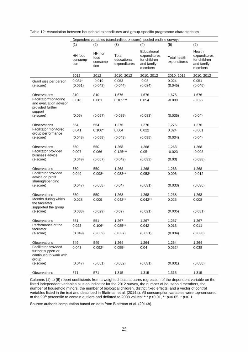
25

Table 12: Association between household expenditures and group-specific programme characteristics

Dependent variables (standardized z-score), pooled endline surveys

(1) (2) (3) (4) (5) (6)

HH food consump-tion

HH non food consump-tion


Educational expenditures for children and family members

Total health expenditures


2012 2012 2010, 2012 2010, 2012 2010, 2012 2010, 2012

Grant size per person (z-score)

0.084* -0.019 0.053 -0.03 0.024 0.051

(0.051) (0.042) (0.044) (0.034) (0.045) (0.046)

Observations 810 810 1,676 1,676 1,676 1,676

Facilitator/monitoring and evaluation advisor provided further support (z-score)

0.018 0.081 0.105*** 0.054 -0.009 -0.022

(0.05) (0.057) (0.039) (0.033) (0.035) (0.04)

Observations 554 554 1,276 1,276 1,276 1,276

Facilitator monitored group performance (z-score)

0.041 0.106* 0.064 0.022 0.024 -0.001

(0.048) (0.058) (0.043) (0.035) (0.034) (0.04)

Observations 550 550 1,268 1,268 1,268 1,268

Facilitator provided business advice (z-score)

0.007 0.066 0.125*** 0.05 -0.023 -0.008

(0.049) (0.057) (0.042) (0.033) (0.03) (0.038)

Observations 550 550 1,268 1,268 1,268 1,268

Facilitator provided advice on profit sharing/spending (z-score)

0.049 0.098* 0.083** 0.053* 0.006 -0.012

(0.047) (0.058) (0.04) (0.031) (0.033) (0.036)

Observations 550 550 1,268 1,268 1,268 1,268

Months during which the facilitator supported the group (z-score)

-0.028 0.009 0.042** 0.042** 0.025 0.008

(0.038) (0.029) (0.02) (0.021) (0.035) (0.031)

Observations 551 551 1,267 1,267 1,267 1,267

Performance of the facilitator (z-score)

0.023 0.106* 0.085** 0.042 0.018 0.011

(0.049) (0.059) (0.037) (0.031) (0.034) (0.038)

Observations 549 549 1,264 1,264 1,264 1,264

Facilitator provided further support or continued to work with group (z-score)

0.043 0.092* 0.055* 0.04 0.052* 0.038

(0.047) (0.051) (0.032) (0.031) (0.031) (0.038)

Observations 571 571 1,315 1,315 1,315 1,315

Columns (1) to (6) report coefficients from a weighted least squares regression of the dependent variable on the listed independent variables plus an indicator for the 2012 survey, the number of household members, the number of household minors, the number of biological children, district fixed effects, and a vector of control variables listed in the text and described in Blattman et al. (2014a). All consumption variables were top-censored at the 99th percentile to contain outliers and deflated to 2008 values. *** p<0.01, ** p<0.05, * p<0.1.


26

I explore the role of these two group-specific programme characteristics in order to shed light on the possible channels of the treatment impact on consumption. Table 12 suggests that the results are not driven by a pure income effect, since the size of the grant received influences only food expenditures. On the contrary, the active presence of the facilitator is positively correlated with non-food expenditures, particularly educational expenditures.

However, it is not possible to test the actual mechanisms at work or to further disentangle all the channels that might have affected the findings. Indeed, there are other factors that might have played a role in influencing the results on educational expenditures. Labelling the cash transfer for expenditure on business tools and skills training might have had an endorsement effect that highlighted the importance of training/schooling (Benhassine et al. 2015). Also, individuals assigned to receive the grant were more likely to practise a skilled trade after four years, and this better employment opportunity might have increased the perceived returns on education (Heath and Mobarak 2015). In addition, it could be that the greater economic stability achieved by treated individuals through their higher earnings enabled them to have more cognitive resources available for their everyday lives and parenting activities (Chiapa et al. 2016). Besides, the group feature of the intervention increased social interactions among members, and hence might have stimulated positive changes in parents’ behaviours through diffusion of social norms or information (Bobba and Gignoux 2017).

While this group feature might have contributed to the success of the programme, and the inclusion of a reserved quota for females might have helped to reduce certain gender gaps, the insistence that a third of the group’s members must be female might also have played a role in increasing redistributive pressures on women. Women’s receipt of more financial requests from non-family members might explain why, after four years, women assigned to receive the grant did not increase educational expenditures, whereas men assigned to receive the grant increased educational expenditures by 24 per cent (US$32).

References

Akresh, R., D. de Walque, and H. Kazianga (2013). ‘Cash Transfers and Child Schooling: Evidence from a Randomized Evaluation of the Role of Conditionality’. Policy Research Working Paper 6340. Washington, DC: World Bank.

Akresh, R., D. de Walque, and H. Kazianga (2016). ‘Evidence from a Randomized Evaluation of the Household Welfare Impacts of Conditional and Unconditional Cash Transfers Given to Mothers or Fathers’. Policy Research Working Paper 7730. Washington, DC: World Bank.

Almås, I., A. Armand, O. Attanasio, and P. Carneiro (2015). ‘Measuring and Changing Control: Women’s Empowerment and Targeted Transfers’. NBER Working Paper 21717. Cambridge, MA: National Bureau of Economic Research.

Alzua, M., G. Cruces, and L. Ripani (2013). ‘Welfare Programs and Labor Supply in Developing Countries: Experimental Evidence from Latin America’. Journal of Population Economics, 26(4): 1255–84.

Angelucci, M., and G. De Giorgi (2009). ‘Indirect Effects of an Aid Program: How Do Cash Transfers Affect Ineligibles’ Consumption?’ American Economic Review, 99: 486–508.

Arcand, J.L., and M. Fafchamps (2012). ‘Matching in Community-Based Organizations’. Journal of Development Economics, 98(2): 203–19.

27

Attanasio, O., E. Battistin, and A. Mesnard (2011). ‘Food and Cash Transfers: Evidence from Colombia’. The Economic Journal, 122: 92–124.

Attanasio, O., and V. Lechene (2002). ‘Test of Income Pooling in Household Decisions’. Review of Economic Dynamics, 5(4): 720–48.

Attanasio, O., and V. Lechene (2014). ‘Efficient Responses to Targeted Cash Transfers’. Journal of Political Economy, 122(1): 178–222.

Baird, S., C. McIntosh, and B. Özler (2011). ‘Cash or Condition? Evidence from a Cash Transfer Experiment’. Quarterly Journal of Economics, 126(4): 1709–53.

Baland, J.M., I. Bonjean, C. Guirkinger, and R. Ziparo (2016). ‘The Economic Consequences of Mutual Help in Extended Families’. Journal of Development Economics, 123: 38–56.

Bandiera, O., N. Buehren, R. Burgess, M. Goldstein, S. Gulesci, I. Rasul, and M. Sulaimany (2015). ‘Women’s Empowerment in Action: Evidence from a Randomized Control Trial in Africa’. Discussion Paper 50. London: STICERD Economic Organization and Public Policy Programme.

Banerjee, A., and E. Duflo (2007). ‘The Economic Lives of the Poor’. Journal of Economic Perspectives, 21(1): 141–67.

Banerjee, A., R. Hanna, G. Kreindler, and B. Olken (2015). ‘Debunking the Stereotype of the Lazy Welfare Recipient: Evidence from Cash Transfer Programs Worldwide’. Available at: economics.mit.edu/files/10861 (accessed 12 April 2017).

Bazzi, S., S. Sumarto, and A. Suryahadi (2015). ‘It’s All in the Timing: Cash Transfers and Consumption Smoothing in a Developing Country’. Journal of Economic Behavior and Organization, 119: 267–88.

Beber, B., and C. Blattman (2013). ‘The Logic of Child Soldiering and Coercion’. International Organization, 67(1): 65–104.

Benhassine, N., F. Devoto, E. Duflo, P. Dupas, and V. Pouliquen (2015). ‘Turning a Shove into a Nudge? A “Labeled Cash Transfer” for Education’. American Economic Journal: Economic Policy, 7(3): 86–125.

BenYishay, A., M. Jones, F. Kondylis, and A. Mobarak (2016). ‘Are Gender Differences in Performance Innate or Socially Mediated?’ Policy Research Working Paper 7689. Washington, DC: World Bank.

Berge, L., K. Juniwaty, and L. Sekei (2016). ‘Gender Composition and Group Dynamics: Evidence from a Laboratory Experiment with Microfinance Clients’. Journal of Economic Behavior and Organization, 131: 1–20.

Björkman, M., and J. Svensson (2009). ‘Power to the People: Evidence from a Randomized Field Experiment on Community-Based Monitoring in Uganda’. Quarterly Journal of Economics, 124(2): 735–69.

Blattman, C., and J. Annan (2010). ‘The Consequences of Child Soldiering’. Review of Economics and Statistics, 92(4): 882–98.

Blattman, C., M. Emeriau, and N. Fiala (2016). ‘Do Anti-Poverty Programs Sway Voters? Experimental Evidence from Uganda’. Available at: papers.ssrn.com/sol3/papers.cfm?abstract_id=2887752 (accessed 12 April 2017).

Blattman, C., N. Fiala, and S. Martinez (2012). ‘Employment Generation in Rural Africa: Mid-Term Results from an Experimental Evaluation of the Youth Opportunities Program in

http://economics.mit.edu/files/10861

https://papers.ssrn.com/sol3/papers.cfm?abstract_id=2887752

28

Northern Uganda’. DIW Berlin Discussion Paper 1201. Berlin: German Institute for Economic Research.

Blattman, C., N. Fiala, and S. Martinez (2014a). ‘Generating Skilled Self-Employment in Developing Countries: Experimental Evidence from Uganda’. Quarterly Journal of Economics, 129(2): 697–752.

Blattman, C., N. Fiala, and S. Martinez (2014b). ‘Northern Uganda Social Action Fund: Youth Opportunities Program’. Harvard Dataverse, V1. Available at: dx.doi.org/10.7910/DVN/27898 (accessed 12 April 2017).

Bobba, M., and J. Gignoux (2017). ‘Neighborhood Effects in Integrated Social Policies’. World Bank Economic Review, forthcoming.

Bold, T., M. Kimenyi, G. Mwabu, and J. Sandefur (2015). ‘Can Free Provision Reduce Demand for Public Services? Evidence from Kenyan Education’. World Bank Economic Review, 29(2): 293–326.

Boltz, M., K. Marazyan, and P. Villar (2015). ‘Preference for Hidden Income and Redistribution to Kin and Neighbors: A Lab-in-the-Field Experiment in Senegal’. PSE Working Paper 15. Paris: Paris School of Economics.

Bozzoli, C., T. Brück, and T. Muhumuza (2011). ‘Does War Influence Individual Expectations?’ Economic Letters, 113, 288–91.

Chiapa, C., J. Garrido, and S. Prina (2012). ‘The Effect of Social Programs and Exposure to Professionals on the Educational Aspirations of the Poor’. Economics of Education Review, 31(1): 778–98.

Chiapa, C., P. Prina, and A. Parker (2016). ‘The Effects of Financial Inclusion on Children’s Schooling, and Parental Aspirations and Expectations’. Journal of International Development, 28(5): 683–96.

Cho, Y., D. Kalomba, A. Mobarak, and V. Orozco (2013). ‘Gender Differences in the Effects of Vocational Training: Constraints on Women and Drop-out Behavior’. Policy Research Working Paper 6545. Washington, DC: World Bank.

Cruz, M., and Z. Ziegelhöfer (2014). ‘Beyond the Income Effect: Impacts of Conditional Cash Transfer Programs on Private Investments in Human Capital’. Policy Research Working Paper 6867. Washington, DC: World Bank.

De Brauw, A., D. Gilligan, J. Hoddinott, and S. Roy (2014). ‘The Impact of Bolsa Familia on Women’s Decision-Making Power’. World Development, 59: 487–504.

Deininger, K. (2003). ‘Does Cost of Schooling Affect Enrollment by the Poor? Universal Primary Education in Uganda’. Economics of Education Review, 22: 291–305.

Duflo, E. (2003). ‘Grandmothers and Granddaughters: Old-Age Pensions and Intra-Household Allocation in South Africa’. World Bank Economic Review, 17(1): 1–25.

Duflo, E. (2012). ‘Women Empowerment and Economic Development’. Journal of Economic Literature, 50(4): 1051–79.

Duflo, E., and C. Udry (2004). ‘Intra-Household Resource Allocation in Cote d’Ivoire: Social Norms, Separate Accounts, and Consumption Choices’. NBER Working Paper 104498. Cambridge, MA: National Bureau of Economic Research.

Fiala, N. (2015a). ‘Business Is Tough, But Family Is Worse: The Role of Family Constraints on Microenterprise Development in Uganda’. Unpublished paper.

http://dx.doi.org/10.7910/DVN/27898

29

Fiala, N. (2015b). ‘The Economic Consequences of Forced Displacement’. Journal of Development Studies, 51(10): 1275–93.

Fiala, N., and X. He (2016). ‘Unitary or Noncooperative Intrahousehold Model? Evidence from Couples in Uganda’. World Bank Economic Review, 30: S77–85.

Fizbein, A., N. Schady, F. Ferreira, M. Grosh, N. Keleher, P. Olinto, and E. Skoufias (2009). ‘Conditional Cash Transfers: Reducing Present and Future Poverty’. Policy Research Report 47603. Washington, DC: World Bank.

Gertler, P., S. Martinez, and M. Rubio-Codina (2012). ‘Investing Cash Transfers to Raise Long-Term Living Standards’. American Economic Journal: Applied Economics, 4(1): 164–92.

Grimm, M., R. Hartwig, and J. Lay (2016). ‘Does Forced Solidarity Hamper Investment in Small and Micro Enterprises?’ Journal of Comparative Economics, forthcoming.

Handa, S., A. Peterman, B. Davis, and M. Stampini (2009). ‘Opening up Pandora’s Box: The Effect of Gender Targeting and Conditionality on Household Spending Behavior in Mexico’s Progresa Program’. World Development, 37(6): 1129–42.

Haushofer, J., and J. Shapiro (2016). ‘The Short-Term Impact of Unconditional Cash Transfers to the Poor: Experimental Evidence from Kenya’. Quarterly Journal of Economics, 131(4): 1973–2042.

Heath, R., and M. Mobarak (2015). ‘Manufacturing Growth and the Lives of Bangladeshi Women’. Journal of Development Economics, 115: 1–15.

Jakiela, P., and O. Ozier (2016). ‘Does Africa Need a Rotten Kin Theorem? Experimental Evidence from Village Economies’. Review of Economic Studies, 83(1): 231–68.

Karlan, D., and L. Linden (2014). ‘Loose Knots: Strong versus Weak Commitments to Save for Education in Uganda’. NBER Working Paper 19863. Cambridge, MA: National Bureau of Economic Research.

Kazianga, H., and Z. Wahhaj (2016). ‘Intra-Household Resource Allocation and Familial Ties’. CSAE Working Paper 6. Oxford: Centre for the Study of African Economies.

Kugler, A., M. Kugler, J. Saavedra, and L. Herrera-Prada (2015). ‘Long-Term Direct and Spillover Effects of Job Training: Experimental Evidence from Colombia’. NBER Working Paper 21607. Cambridge, MA: National Bureau of Economic Research.

LaFave, D., and D. Thomas (2017). ‘Extended Families and Child Well-Being’. Journal of Development Economics, 126: 52–65.

Macours, K., N. Schady, and R. Vakis (2012). ‘Cash Transfers, Behavioral Changes, and the Cognitive Development of Young Children: Evidence from a Randomized Experiment’. American Economic Journal: Applied Economics, 4(2): 247–73.

Macours, K., and R. Vakis (2014). ‘Changing Households’ Investment Behaviour through Social Interactions with Local Leaders: Evidence from a Randomized Transfer Programme’. The Economic Journal, 124: 607–33.

Maluccio, J., and A. Quisumbing (2003). ‘Resources at Marriage and Intra-Household Allocation: Evidence from Bangladesh, Ethiopia, Indonesia, and South Africa’. Oxford Bulletin of Economics and Statistics, 65(3): 283–327.

Peterman, A., B. Schwab, S. Roy, M. Hidrobo, and D. Gilligan (2015). ‘Measuring Women’s Decision-Making: Indicator Choice and Survey Design Experiments from Cash and Food Transfer Evaluations in Ecuador, Uganda, and Yemen’. Discussion Paper 1453. Washington, DC: International Food Policy Research Institute.

30

Quisumbing, A., N. Kumar, and J. Behrman (2011). ‘Do Shocks Affect Men’s and Women’s Assets Differently? A Review of Literature and New Evidence from Bangladesh and Uganda’. Background Paper to the World Development Report 2012. Washington, DC: World Bank.

Ruvalcava, L., G. Teruel, and D. Thomas (2009). ‘Investments, Time Preferences, and Public Transfers Paid to Women’. Economic Development and Cultural Change, 57(3): 507–38.

Saavedra, J.E., and S. Garcia (2012). ‘Impacts of Conditional Cash Transfer Programs on Educational Outcomes in Developing Countries: A Meta-Analysis’. Working Paper 921. Santa Monica, CA: Rand Corporation.

Schady, N., and J. Rosero (2008). ‘Are Cash Transfers Made to Women Spent Like Other Sources of Income?’ Economics Letters, 101(3): 246–48.

Shah, M., and B. Steinberg (2015). ‘Workfare and Human Capital Investment: Evidence from India’. NBER Working Paper 21543. Cambridge, MA: National Bureau of Economic Research.

Thomas, D. (1990). ‘Intra-Household Resource Allocation: An Inferential Approach’. Journal of Human Resources, 25(4): 635–64.

Thomas, D. (1993). ‘The Distribution of Income and Expenditure within the Household’. Annales d’Economie et de Statistique, 29: 109–36.

Tommasi, D. (2016). ‘How Cash Transfers Improve Child Development’. Available at: papers.ssrn.com/sol3/papers.cfm?abstract_id=2610515 (accessed 12 April 2017).

Voors, M., E. Nillesen, P. Verwimp, E. Bulte, R. Lensink, and D. Van Soest (2012). ‘Violent Conflict and Behavior: A Field Experiment in Burundi’. American Economic Review, 102(2): 941–64.

World Bank (2009). ‘Implementation Completion and Results Report of the Northern Uganda Social Action Fund’. Report ICR1211. Washington, DC: World Bank. Available at: documents.worldbank.org/curated/en/417791468310732815/pdf/ICR12110P002951IC0disclosed03111101.pdf (accessed 14 April 2017).

World Bank (2014). ‘World Development Indicators 2014’. Washington, DC: World Bank. Available at: data.worldbank.org/data-catalog/world-development-indicators (accessed 14 April 2017).

Yoong, J., L. Rabinovich, and S. Diepeveen (2012). ‘The Impact of Economic Resource Transfers to Women versus Men: A Systematic Review’. EPPI-Centre Technical Report. London: University College London, Institute of Education, Social Science Research Unit.

Zhou, W. (2015). ‘The Intergenerational Impact of Early Life Adversity: Evidence from the Send-Down Policy in China’. Available at: editorialexpress.com/cgi-bin/conference/download.cgi?db_name=NEUDC2015&paper_id=398 (accessed 12 April 2017).

https://papers.ssrn.com/sol3/papers.cfm?abstract_id=2610515

http://documents.worldbank.org/curated/en/417791468310732815/pdf/ICR12110P002951IC0disclosed03111101.pdf

http://documents.worldbank.org/curated/en/417791468310732815/pdf/ICR12110P002951IC0disclosed03111101.pdf

http://data.worldbank.org/data-catalog/world-development-indicators

https://editorialexpress.com/cgi-bin/conference/download.cgi?db_name=NEUDC2015&paper_id=398

https://editorialexpress.com/cgi-bin/conference/download.cgi?db_name=NEUDC2015&paper_id=398

WIDER Working Paper 2017/93

Documents

Transcript of WIDER Working Paper 2017/93