General rights Copyright and moral rights for the publications made accessible in the public portal are retained by the authors and/or other copyright owners and it is a condition of accessing publications that users recognise and abide by the legal requirements associated with these rights.

• Users may download and print one copy of any publication from the public portal for the purpose of private study or research. • You may not further distribute the material or use it for any profit-making activity or commercial gain • You may freely distribute the URL identifying the publication in the public portal

If you believe that this document breaches copyright please contact us providing details, and we will remove access to the work immediately and investigate your claim.

Downloaded from orbit.dtu.dk on: May 11, 2018

Why is it so difficult to determine the lateral Position of the Rails by a Measurement ofthe Motion of an Axle on a moving Vehicle?

True, Hans; Christiansen, Lasse Engbo

Published in:Proceedings of First International Conference on Rail Transportation 2017

Publication date:2017

Document VersionPublisher's PDF, also known as Version of record

Link back to DTU Orbit

Citation (APA):True, H., & Christiansen, L. E. (2017). Why is it so difficult to determine the lateral Position of the Rails by aMeasurement of the Motion of an Axle on a moving Vehicle? In Proceedings of First International Conference onRail Transportation 2017

First International Conference on Rail Transportation

Chengdu, China, July 10-12, 2017

Why is it so difficult to determine the lateral Position of the Rails by a Measurement of the Motion of an Axle on a moving Vehicle? Hans TRUE, and Lasse Engbo CHRISTIANSEN

DTU Compute, The Technical University of Denmark, DK-2800 Kgs.Lyngby, Denmark Abstract: Several attempts of measuring the exact location of the rails by the use of ordinary vehicles have been made. While the method works reasonably well in the vertical direction, the results of the lateral measurements made with different vehicles are so widely scattered that it is virtually impossible to draw any conclusions. We may therefore ask: does a wheel set follow the track disturbances exactly? In this article we investigate the lateral dynamics of a half-car vehicle model with two-axle bogies running on a rigid tangent track with sinusoidal lateral disturbances of the rails. The wavelength, the amplitude and the phase between the rail disturbances are varied. Two different vehicle speeds are investigated. One speed is under and the other above the vehicle critical speed. In the article we show examples of axle motions that do not follow the track disturbances in phase, amplitude or period or several of these together. The results are discussed, and we must conclude that it is in general impossible to determine the track geometry from the motion of a wheel set. Keywords: Train-Track Interaction; Railway Vehicle Dynamics; Vehicle-Track coupled Dynamics

1 Introduction There is today a great interest in measurements of the quality of railway tracks by instrumentation of vehicles in normal use. Weston et al. [1] wrote a survey article on the subject with 59 references. Usually the motion or acceleration of a wheel set or an axle box is recorded and used either directly or indirectly for a determination of the track quality. If, however, the wheel sets do not follow the disturbances of the track accurately, then the recordings do not deliver a trustworthy basis for the evaluation of the quality of the track. We only know of two systematic investigations of the response of wheel sets to a disturbed track. Meijaard and De Pater [2] investigated theoretically the dynamics of the rolling motion of a simple model of a wheel set on a sinusoidal laterally deformed track. They found both periodic and chaotic motions. Lieh and Haque [3] calculated the stability and instability regions for a single wheel set subject to variations in the wheel-rail geometry, track gauge and axle load. They showed that harmonic variations in the

wheel-rail geometry can influence the behavior of a wheel set significantly. In the conclusion Lieh and Haque [3] write that the behavior of their wheel set is similar to a single-degree-of-freedom system and that parametric resonance occurs when the frequency of excitation is twice or some multiple of the kinematic or Klingel frequency. The lateral motion of the wheel set is, however, coupled with the yaw motion, so in reality the behavior is similar to a double-degree-of-freedom system. Time varying systems with multiple degrees-of-freedom may in addition experience resonance for some combinations of their natural frequencies. We therefore investigate the response of a simplified model of a half-vehicle running on a track with a realistic and well-proven wheel-rail interaction model. We have chosen the Cooperrider bogie, because its dynamics is well-known from earlier papers [4,5,6,7], but we have extended the model to include vertical degrees of freedom. The speed of the vehicle, the wavelength and the amplitude of the sinusoidal laterally disturbed track all enter the problem as control parameters and we

First International Conference on Rail Transportation 2017

have investigated lateral track centerline variations and gauge variations at a speed below and at a speed above the critical speed. Some results are presented and the effects on the track quality estimates are discussed.

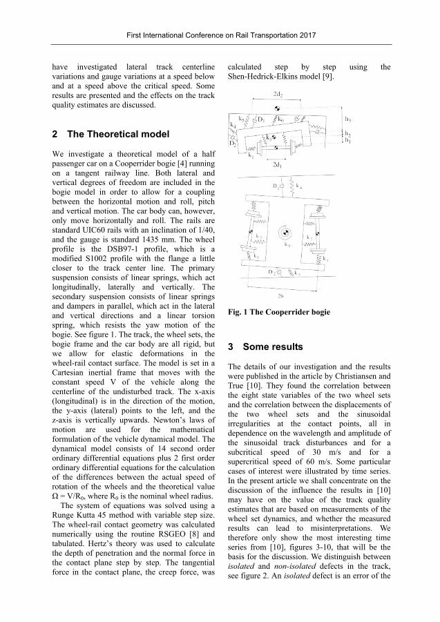
2 The Theoretical model We investigate a theoretical model of a half passenger car on a Cooperrider bogie [4] running on a tangent railway line. Both lateral and vertical degrees of freedom are included in the bogie model in order to allow for a coupling between the horizontal motion and roll, pitch and vertical motion. The car body can, however, only move horizontally and roll. The rails are standard UIC60 rails with an inclination of 1/40, and the gauge is standard 1435 mm. The wheel profile is the DSB97-1 profile, which is a modified S1002 profile with the flange a little closer to the track center line. The primary suspension consists of linear springs, which act longitudinally, laterally and vertically. The secondary suspension consists of linear springs and dampers in parallel, which act in the lateral and vertical directions and a linear torsion spring, which resists the yaw motion of the bogie. See figure 1. The track, the wheel sets, the bogie frame and the car body are all rigid, but we allow for elastic deformations in the wheel-rail contact surface. The model is set in a Cartesian inertial frame that moves with the constant speed V of the vehicle along the centerline of the undisturbed track. The x-axis (longitudinal) is in the direction of the motion, the y-axis (lateral) points to the left, and the z-axis is vertically upwards. Newton’s laws of motion are used for the mathematical formulation of the vehicle dynamical model. The dynamical model consists of 14 second order ordinary differential equations plus 2 first order ordinary differential equations for the calculation of the differences between the actual speed of rotation of the wheels and the theoretical value Ω = V/R0, where R0 is the nominal wheel radius.

The system of equations was solved using a Runge Kutta 45 method with variable step size. The wheel-rail contact geometry was calculated numerically using the routine RSGEO [8] and tabulated. Hertz’s theory was used to calculate the depth of penetration and the normal force in the contact plane step by step. The tangential force in the contact plane, the creep force, was

calculated step by step using the Shen-Hedrick-Elkins model [9].

Fig. 1 The Cooperrider bogie

3 Some results The details of our investigation and the results were published in the article by Christiansen and True [10]. They found the correlation between the eight state variables of the two wheel sets and the correlation between the displacements of the two wheel sets and the sinusoidal irregularities at the contact points, all in dependence on the wavelength and amplitude of the sinusoidal track disturbances and for a subcritical speed of 30 m/s and for a supercritical speed of 60 m/s. Some particular cases of interest were illustrated by time series. In the present article we shall concentrate on the discussion of the influence the results in [10] may have on the value of the track quality estimates that are based on measurements of the wheel set dynamics, and whether the measured results can lead to misinterpretations. We therefore only show the most interesting time series from [10], figures 3-10, that will be the basis for the discussion. We distinguish between isolated and non-isolated defects in the track, see figure 2. An isolated defect is an error of the

First International Conference on Rail Transportation 2017

track geometry that creates a dynamic transient motion of the wheel set, which disappears before the next error is encountered by the wheel set. Non-isolated or continuous defects are defined as errors that are so densely distributed that the wheel set will encounter more than one defect within its response time, which is the time it takes for the response to an isolated defect to disappear. The definitions are not uniquely

related to the track properties, because the nonlinear wheel set response gives rise to mode interactions that depend on the specific vehicle design as well as the excitation that is caused by the defects. Since a lateral sinusoidal disturbance obviously is a non-isolated defect, we do not discuss the effect of isolated disturbances in this article.

Fig. 2 An illustration of the response to isolated irregularities. Each irregularity is modelled as a missing chip that is 10 mm long and 2 mm deep (marked by vertical dotted lines). The full line shows the lateral motion of the front wheel set, and the dashed line shows the yaw angle of the front wheel set.

First International Conference on Rail Transportation 2017

Fig. 3 The motion of the leading wheel set relative to the track centerline variations with the wavelength 30 m at V=30 m/s. The bold line indicates the position of the rail, the full line shows the lateral position and the dashed line the yaw angle of the leading wheel set. On (c) notice the asymmetric oscillation of the wheel set in the track.

First International Conference on Rail Transportation 2017

Fig. 4 The motion of the leading wheel set relative to the track centerline variations with the wavelength 10 m at V=30 m/s. The bold line indicates the position of the rail, the full line shows the lateral position and the dashed line the yaw angle of the leading wheel set. In case (e) a longer transient was needed to find the equilibrium solution with its apparently non-periodic oscillatory behavior. (f) is a phase portrait of the motion with indication of chaos

First International Conference on Rail Transportation 2017

Fig. 5 The motion of the leading wheel set relative to the track centerline variations. In (a) and (b) the wavelength of the disturbance 2.5 m, and in (c) and (d) it is 5 m. V=30 m/s. The bold line indicates the position of the rail, the full line shows the lateral position and the dashed line the yaw angle of the leading wheel set

Fig. 6 The motion of the wheel set relative to the gauge variations of the track. The bold line indicates the position of the left rail, the full line shows the lateral position and the dashed line the yaw angle of the leading wheel set. V=30 m/s and the wavelength is 5 m. Notice the period of the response of the wheel set, which is twice the period of the excitation, and the jump of the amplitudes of the motion of the wheel set between case (a) and case (b)

First International Conference on Rail Transportation 2017

Fig. 7 The motion of the wheel set relative to the gauge variations of the track. The bold line indicates the position of the left rail, the full line shows the lateral position and the dashed line the yaw angle of the leading wheel set for different wavelengths of the forcing. V=30 m/s and the forcing amplitude is 5 mm

First International Conference on Rail Transportation 2017

Fig. 8 The motion of the wheel set relative to the gauge variations of the track. The bold line indicates the position of the left rail, the full line shows the lateral position and the dashed line the yaw angle of the leading wheel set for different wavelengths of the forcing. V=30 m/s and the forcing amplitude is 5 mm.

First International Conference on Rail Transportation 2017

Fig. 9 Three time series with centerline irregularities and with a speed of 60 m/s. A transient of 100 s was allowed. The motion of the wheel set relative to the position of the track. The bold line indicates the position of the track, the full line shows the lateral position and the dashed line the yaw angle of the leading wheel set for different wavelengths and amplitudes of the forcing.

First International Conference on Rail Transportation 2017

Fig. 10 Five time series with gauge irregularities and a speed of 60 m/s. The forcing amplitude is 5.5 mm. On the figures (a) to (e) the bold line indicates the position of the left rail, the full line shows the lateral position and the dashed line the yaw angle of the leading wheel set. (f) shows a phase portrait of the motion on (e).

4 Discussion We start with a vehicle speed of 30 m/s and consider first examples of center line disturbances. Let us look at figure 3. It shows a very fine correlation between the

period and phase of the track center line disturbance and the front wheel set displacement. The amplitudes are different, however. The wheel set amplitude is larger, and it grows with the

First International Conference on Rail Transportation 2017

amplitude of the disturbance, but the factor of amplification is decreasing (notice the different length scales on the figures). On figure 4 only the period is the same. Between a disturbance amplitude of 1 mm and 2.5 mm the wheel set amplitude jumps from being smaller to being larger than the disturbance amplitude and the phase difference changes with the disturbance amplitude from a phase lag π over π /2 (correlation 0) to a small phase lag. The shape of the wheel set oscillation changes from sinusoidal over no longer sinusoidal but still periodic to presumably chaotic with a not- well defined amplitude. A correction of the track geometry based on the wheel set displacement would lead to a deterioration of the track quality, when the track errors are small. On figure 5 the periods are the same, but the wheel set amplitude is indistinguishable from 0 when the wavelength is 2.5 m and much smaller than the track disturbance amplitude when the wavelength is 5 m. Furthermore there is a phase lag of π between the track and wheel set displacements, and the periodic motion of the wheel set becomes non-sinusoidal with larger amplitudes of the track disturbance. A correction of the track geometry based on the wheel set displacement would not be made (see figures 5(a) and 5(b)) or lead to a deterioration (see figure 5(c)) or would be insufficient (see figure 5d)).

Next we look at examples of gauge disturbances. The magnitude of the disturbance is defined by the amplitude of the left rail. We only consider amplitudes less than 6 mm corresponding to gauge changes of ±12 mm, which is already larger than the allowed maximal gauge change. On figure 6 we find that the wavelength of the wheel set oscillations is twice the one of the gauge oscillations and for growing amplitude of the gauge

oscillations the amplitude of the wheel set oscillations becomes larger than the gauge oscillations and change shape. On figure 7 we find that for small wavelengths the amplitude of the wheel set oscillations are larger than the gauge oscillations, and the wavelength is again twice the one of the gauge oscillations. For the 10 m wavelength of the gauge disturbance the wheel set oscillations vanish, and for 12.5 m wavelength of the gauge disturbance the wheelset oscillation has larger amplitude than the gauge disturbance and is off-set from the track center line. The wave lengths of the gauge and wheel set oscillations are now the same. On figure 8, notice that all oscillations of the wheel set, except (d) are off-set with amplitudes that are smaller than the amplitudes of the gauge disturbances. For the wavelength of 15 m we find a period doubling, which results in a period 2:2 motion. Two periods of the forcing as well as of the lateral oscillation of the wheel set are needed before the motion is repeated. For the disturbance wavelength 17.5 m the motion is 1:1 periodic with a phase difference of π with an amplitude, which is reduced when the wavelength is increased to 20 m and still more reduced when the disturbance wavelength grows to 22.5 m, where the oscillation of the leading wheel set vanishes (see figures 8(b) to 8(d)). On figure 8(e) we find an interesting 2:3 synchronized motion. First the wheel set moves 2.5 mm to the left, then it makes a small and fast oscillation to the right, returns to the left with small amplitude ending with a 2.5 mm move to the right. This type of behavior is repeated for a wavelength of 27.5 m, but the amplitudes decrease, see figure 8(f). The next figures show some results when the speed is doubled to 60 m/s, which is above the critical speed of the vehicle.

First International Conference on Rail Transportation 2017

Then the excitation frequency from the track is twice the former excitation frequency. The speed lies in the range of the two co-existing attractors i.e. below the bifurcation point of the steady motion. First we investigate center line variations. On figure 9 we again find an amplification factor of the wheel set oscillations that depends on the wavelength of the forcing. On figure 9(a) we see what might be a period 8:3 synchronization, but the transient has not yet vanished. On figure 9(b) a period 7:4 synchronization is seen, and on figure 9(c) the transient has not vanished, or the period of the wheel set oscillations is longer than the 30 oscillations of the forcing that are shown on the figure. It is worth mentioning that the observed synchronizations result in a wheel set oscillation with a primary frequency that is close to what was observed for the same wavelengths at 30 m/s and thus independent of the Klingel frequency. We also investigated the effect of gauge variations shown on figure 10. The forcing amplitude is now 5.5 mm. On figure 10(a) we observe a motion that is very similar to the period 2:1 motion on figure 7(a), but 10(a) is a period 2:5 motion. For a wavelength of 20 m, see figure 10(b), the period 1:1 motion seems similar to a case between wavelengths of 17.5 m and 20 m on figure 8. For a wavelength of 30 m, see figure 10(c), we observe a period 2:3 motion like the one on figure 8(e), where the forcing wavelength is 25 m. When the forcing wavelength grows to 32.5 m the wheel set oscillation vanishes, and when the forcing wavelength is 35 m, see figure 10(e), a period 2:5 solution appears. The change of dynamics from the 2:3 case consists of an extra swing of the largest amplitude of the motion. The extra swing is clearly seen as the small loops on the phase portrait on figure 10(f).

We have only shown examples of behaviors of the wheel set that differ strongly from the forcing sinusoidal variations of the track. There are of course also large parameter domains in which the wheel set oscillations follow the forcing better. For a more detailed description and many more results, the reader is referred to the article by Christiansen and True [10]. The examples shown in this article demonstrate that it is very difficult, indeed impossible, to draw any conclusions about the lateral track geometry from measurements of the axle displacements of an in-service railway vehicle alone.

It has been suggested to add a numerical routine that can solve the inverse problem: Given the dynamics of the wheel set, then use the data to determine the track geometry. Linear relations have been set up as a solver to the inverse problem, but they are doomed to fail because they miss the nonlinear relations that are necessary for the formulation of the dynamic mode interactions. The dynamical problem: to find the dynamic response of a wheel set to external forcing involves the entire vehicle due to the nonlinear couplings. Therefore the inverse problem involves the data of the dynamics of the entire vehicle, and it is still an open question whether such an inverse problem can be solved with a unique solution. The problem is to find the inverse operator of a nonlinear and non-smooth operator. The figures 7(c), 8(d) and 10(d) demonstrate that a unique solution to the inverse problem does not exist in certain cases, because the ‘no- displacements’ of the wheel set in all three cases are the same as the ‘no-displacement’on an undisturbed track. Therefore in each case two entirely different track geometries lead to the same solution. The inverse problem therefore has two different

First International Conference on Rail Transportation 2017

solutions: 1: the track is perfect and 2: the track is sinusoidally disturbed. How can the solver distinguish between them? This problem is mathematical. The question is: Does the inverse operator exist and if not in general, then under which conditions does it exist? Is the solution unique and if not, which extra conditions will make the correct solution unique? This question needs an answer in order to justify further investments in the measurements of the track geometry by in- service vehicles. 5 Conclusions The easy answer to the question in the title is that the wheel set does not follow the lateral track geometry closely. It is more difficult to understand ‘why’. The vertical dynamics of the wheel set is very similar to a single-degree-of-freedom system with a mass under the influence of gravity that forces the wheel set to remain in contact with the track. A vertical track disturbance causes only very small additional vertical penetrations of the wheel set into the rails and acts only on one component of the contact force: the normal component. The lateral disturbance in contrast acts on the lateral force as well as on the spin torque in dependence on the creepage and the non-smoothness due to the contact geometry. Furthermore the lateral and yaw restoring forces consist of relatively small suspension forces and the gravitational stiffness, which all act on bodies with large inertia with a resulting time lag of their motion. Finally the wheel-rail contact design permits larger displacements of the wheel sets relative to the track in the lateral than in the vertical direction. The horizontal motion of the wheel set is similar to a system of two nonlinearly coupled oscillators, because the lateral displacement of the

wheel set is intimately coupled with the yaw. The coupling is a result of the rail and wheel profile geometries, the creep force and the spin from each wheel that all act simultaneously on the wheel set. The forces and torques are nonlinearly dependent on the creepage and they are non-smooth due to the contact geometry. References Weston P., Roberts G., Yeo G. and Stewart

E. 2015. Perspectives on railway track geometry condition monitoring from in-service railway vehicles. Vehicle System Dynamics, 53: 1063-1091.

Meijaard J.P. and dePater A.D. 1989. Railway vehicle system dynamics and chaotic vibrations. International Journal of Non-linear Mechanics, 24: 1-17.

Lieh J. and Haque I. 1988. Parametrically excited behavior of a railway wheelset. Journal of Dynamic Systems, Measurement and Control, 110: 8-17.

Cooperrider N.K. 1972. The hunting behavior of conventional railway trucks. ASME J. Engineering and Industry, 94:752-762.

True H. and Kaas-Petersen C. 1984. A Bifurcation Analysis of Nonlinear Oscillations in Railway Vehicles. Proc. 8th IAVSD Symposium on Vehicle System Dynamics, Swets & Zeitlinger, Lisse.655-665.

Isaksen P. and True H. 1997. On the ultimate transition to chaos in the dynamics of Cooperrider’s bogie. Chaos, Solitons and fractals, 8(4): 559-581.

Nordstrom Jensen C. and True H. 1997. On a new route to chaos in railway dynamics. Nonlinear Dynamics,13:117-129.

Kik W. 2001 RSGEO. http://www.argecare.de/produkte.htm.

Shen Z.Y., Hedrick J.K. and Elkins J.A. 1984. A comparison of alternative creep-force models for rail vehicle dynamical analysis. Proc. 8th IAVSD Symposium on Vehicle System Dynamics, Swets & Zeitlinger, Lisse 591-605.

Christiansen L.E. and True H. 2017. On the dynamics of a railway vehicle on a laterally disturbed track. Submitted to Vehicle System Dynamics.