Why IMF Stabilization Programs Fail To Prevent Currency Crises in Some Financially Distressed Countries But Not Others?*

Bumba Mukherjee Assistant Professor

Dept. of Political Science and Dept. of Economics & Econometrics University of Notre Dame

Visiting Associate Research Scholar CGG, Woodrow Wilson School

Princeton University smukherj@Princeton.edu

Abstract: A critical function of the International Monetary Fund (IMF) is to prevent currency crises in the international monetary system. Yet recent episodes of currency crashes and a dataset on currency crises in 82 countries (1974-2002) reveal that the IMF’s short-term stabilization program –which is explicitly designed to prevent currency crashes -- failed to prevent currency crises in some but certainly not all (i.e. most) of the financially distressed countries that participated in the stabilization program. What explains this variation? I construct a model of speculative trading that examines how the IMF’s ability to prevent currency crashes via its stabilization program crucially depends on the degree of institutionalized state intervention in the financial sector of countries that participate in the IMF’s stabilization program. The model predicts that the greater (lesser) the extent of institutionalized state intervention in the financial sector of a financially troubled country that participates in the IMF’s stabilization program, the harder (easier) it is for that country to credibly commit ex ante to financial sector reforms, as required by the stabilization program. Weak (strong) commitment to IMF reforms increases (decreases) the incentives for currency traders to engage in a speculative attack against the country’s currency and this increases (decreases) the likelihood of a currency crisis. Results from Spatial Autoregressive (SAE) Bivariate Probit models provide strong statistical support for the model’s main prediction.

* Note: An earlier version of this paper was presented at the IMF. The findings presented in this paper do not represent the IMF’s views on this issue. I thank Sergio Bejar for research assistance. The usual disclaimer applies.

1

1. Introduction

The 1990s and the early years of this decade were turbulent times in the international

monetary system. The turbulence began with hyperinflation in the former Soviet bloc, passed

through the Tequila crisis in Mexico in 1994 and was followed by successive financial crises –

characterized by currency crashes – in Thailand, Indonesia and Malaysia. It then spread to Russia

where the rouble collapsed in 1998 and was transmitted to Argentina, Brazil, Uruguay and

Turkey. The costs of the financial crises in the affected countries were devastating: savings were

wiped out, millions of jobs were eliminated in few days, several families were confronted with

the grim reality of poverty and food riots occurred regularly. Moreover, the crisis led to a bloody

civil strife in Indonesia, fostered the resurgence of anti-democratic forces in Russia and

engendered serious political instability in other affected countries.

With each successive crisis, policy-makers, academics and the media increasingly

accused the International Monetary Fund (IMF) of negligence and asked why it could not

prevent these crises? After all, the critics suggested that since the IMF is obliged by Article

IV of its own constitution to minimize currency crashes, it should have prevented the

currency crises that occurred. Some critics even charged that the conditional loans provided

by the IMF to ostensibly prevent a currency crisis in financially “distressed” countries –

suffering from severe balance of payments problems, high external debt and low reserves –

that ironically turned to the IMF for help increased the likelihood of currency collapse in

these countries (Stiglitz 2002; Barro 1999). Officials from the IMF, including its director-

general at the time Stanley Fischer, however, suggested that the anti-IMF accusations were

unfair and that the IMF’s short-run stabilization program (which is different from its long-run

structural adjustment programs) prevented currency crashes and financial catastrophes in

most if not all countries participating in IMF stabilization programs. The recrimination and

finger-pointing between the IMF and its critics triggered the following unresolved debate:

2

Does the IMF’s stabilization program for financially troubled countries increase or decrease

the likelihood of a currency crisis?

With the benefit of hindsight and some preliminary data analysis, we now know

that IMF stabilization programs prevented currency crises in some financially distressed

countries but failed to prevent a currency collapse in other financially troubled countries that

also turned to the IMF for assistance. In fact, a dataset of 82 countries between 1974 and

2002 reveals – the first recorded currency crash in the data, which is described later,

occurred in Argentina in 1975-- that in this time period almost 40% of a total of 531 IMF

short-run stabilization programs for financially distressed countries failed to prevent a

currency crisis, but the remaining 60% of the programs prevented currency crashes. For

instance, the IMF’s stabilization program and conditional financial assistance for Brazil

(March 1999) prevented a speculative attack on their respective currencies and thus

prevented a full-fledged currency crisis. In contrast, IMF programs in Indonesia (1998) and

Russia (1998) ended in unmitigated disaster and could not prevent the collapse of the

Indonesian rupiah and the Russian rouble; this is graphically illustrated in the smoothed

transition probabilities for the Indonesian case in figure 1.

<<Insert figure 1 about here>>

The intriguing finding in my data and the examples mentioned above leads to the central

puzzle addressed in this paper: Why have IMF short-run stabilization programs failed to

prevent currency crises in some financially distressed countries but not others?

Before summarizing my answer to the aforementioned question, let me briefly mention

here that scholars have surprisingly not addressed the issue of why there is substantial variation

in the efficacy of IMF stabilization programs with respect to preventing currency crises. For

instance, several studies have examined the impact of IMF structural adjustment programs on

macroeconomic outcomes such as growth, unemployment, inflation and fiscal deficits

3

(Vreeland 2003; Stone 2002; Dreher & Vaubel 2004a; Hutchison 2003; Fischer 2004; Barro &

Lee 2003). But none of these studies analyze the varied impact that IMF stabilization programs

have on currency markets. Political scientists have also theorized and tested claims about the

impact that domestic political institutions have on the likelihood of currency crises (Leblang

2001, 2003; Leblang and Bernhard 2001; Leblang & Satyanath 2006). While insightful, these

studies ignore the potential impact that the IMF may have in terms of negatively (or positively)

influencing the likelihood of currency crises. In contrast some economists have studied

whether or not IMF conditional loans to financially troubled countries lead to moral hazard

problems (Conway 2002; Knight & Sanaletta 2000). However, instead of studying how IMF

programs affect currency markets, as done here, they restrict their analysis to studying the

effect of IMF programs on domestic equity markets or interest rates in countries that borrow

from the IMF. Finally, the few works on the IMF and crisis-prevention are analytically

insufficient since they only focus on the IMF’s failures in the 1990s, which is tantamount to

sample selection (Desai 2003; Stiglitz 2002).

To answer this paper’s central question posited above, I construct a model of

speculative trading that studies how the IMF’s ability (or inability) to prevent currency

crashes via its stabilization program crucially depends on the degree of institutionalized state

intervention in the financial sector of financially “distressed” countries that participate in the

IMF’s stabilization program. In particular, the formal model presented in this paper studies

how strategic interaction between three actors affects the likelihood of a currency crisis: (i)

the government of a financially distressed country that participates in the IMF’s stabilization

program to avoid a speculative run on its currency (ii) the IMF that provides a short-run

stabilization package to the troubled country conditional on the latter’s promise that it will

implement financial sector reforms and (iii) currency traders that trade the distressed

country’s currency in international capital markets.

4

The model predicts that the greater (lower) the extent of institutionalized state

intervention in the financial sector –captured by the extent of state-ownership of financial

services and its role in financial intermediation – of a financially troubled country that turns

to the IMF for help, the higher (lesser) the likelihood that IMF stabilization program will

foster a currency crisis in that country. Specifically, a higher level of institutionalized state

intervention in the financially troubled country’s financial sector leads to greater political

resistance to financial sector reforms that the IMF attaches as a condition to its stabilization

program. Consequently, the credibility of the government’s commitment to implement ex

post financial sector reforms suggested by the IMF weakens. When the financially troubled

government fails to credibly commit to IMF-requested financial reforms, traders rationally

anticipate that the country’s macroeconomic fundamentals will improve. This, in turn,

provides incentives to traders to opt for a speculative attack against the country’s currency in

a rational expectations equilibrium, which leads to a currency crisis. Conversely, distressed

countries that borrow from the IMF under its stabilization program but have a low degree of

state intervention in the financial sector are more likely to credibly and successfully commit

to implement financial sector reforms ex post. This will reduce the incentives for traders to

engage in a speculative and thus prevent a currency crisis.

I present and estimate an original statistical model in this paper called the spatial

autoregressive error (SAE) bivariate probit model to account for both selection/participation of

financially troubled countries in IMF stabilization programs and spatial dependence in the data

when testing my theoretical claims. Results from the SAE bivariate probit model estimated on a

data set of 82 countries between 1974 and 2002 statistically corroborate my model’s prediction.

The findings presented in this paper have several important implications that are briefly

previewed here but are discussed in more detail in the conclusion. First, more broadly, this paper

is among the first to not only study the impact of IMF programs on currency markets that has

5

been overlooked so far but also carefully address’ variation in the effect of IMF stabilization

programs on preventing currency crises. By doing so, it fills a large gap in the literature since

extant studies almost entirely focus on the effect of IMF programs on macroeconomic

outcomes. Second, a key policy implication of this study is that the IMF should either scale back

or increase the time span for carrying out the financial sector reforms that it requests from

countries that participate in its stabilization program. Indeed, IMF stabilization programs should

not be completely overhauled or stopped, as suggested by several critics.

In the next section I present my model of speculative trading that provides some

testable hypotheses. In sections 3 and 4, I describe the data, variables, statistical

methodology and empirical results. I conclude with a brief summary of the study and discuss

the implications of the research presented in this paper.

2. The model

I present a simple model of speculative trading in this section to examine the

conditions under which IMF short-run stabilization programs are likely to prevent a

currency collapse in financially troubled countries that turn to the IMF for financial help.

Specifically, the formal model presented below studies how interaction between three players

affects the likelihood of a currency crisis: (i) the government of a financially troubled country

– suffering from balance-of-payments and external debt problems -- that participates in the

IMF’s stabilization program to avoid a speculative run on its currency (ii) the IMF that

provides financial aid via a short-run stabilization package to the troubled country

conditional on the latter’s promise that it will implement fiscal policy reforms and (iii)

currency traders/ speculators that trade the troubled country’s currency in capital markets.

The model presented below builds on existing models of currency crises by Morris and Shin

(1998) and Heinemann and Illing (2003), but differs in two key respects.

6

First, unlike existing models of currency crises that ignore either the role of the IMF

or the government of financially troubled/debtor countries, a key innovation of my model is

that it studies how strategic interaction between three players (mentioned above), i.e. the

IMF, currency traders and the financially troubled country, affects the likelihood of a

currency crisis. Second, the model presented here specifically examines how domestic

politics associated with financial sector reforms influences the impact of IMF stabilization

programs on currency markets, which has not been done earlier.

2.1 Players and their Payoff functions

In the model there exists a continuum of currency traders ]1,0[∈i . The traders

strategic choice is to either “attack” or “not attack” the currency of the financially troubled

country based on their expectations of the macroeconomic “fundamentals” in the troubled

country, which is defined by the continuous parameter θ ∈ [0,1]. If a speculative attack is

successful, then traders get the reward r(θ), which is normalized, without loss of generality, to

1. Attacking the currency, however, leads to transaction costs for the currency traders that is

labeled as t. Hence, the net payoff to a trader from a speculative attack is 1− t , while the

payoff to an unsuccessful attack is given by -t.

Note that ex ante traders in international capital markets do not fully know the value

and are thus uncertain about the future state of θ . This is not surprising given that they are

uncertain about whether or not macroeconomic fundamentals will improve ex post in the

financially troubled country after the latter receives financial assistance from the IMF.

However, following extant models (see Morris and Shin 1998; Corsetti et al 2004), each

speculator i observes a private signal si aboutθ with some “noise”:

si = θ + σεi (1)

7

where σ > 0 is a constant1 and the noise termεi is independently and identically distributed

(i.i.d) across traders with density function f (.) and cumulative distribution function F(.).2

Given si, each trader’s strategy is an action that maps the realization of his signal to one of

two actions: attack or not attack the currency in question. In other words, each trader’s

strategy is defined as the function ai : ℜ → {0,1}where ai(si) = 1 indicates that the trader

attacks the country’s currency after observing his signal, while ai(si) = 0 indicates that he

refrains from attacking the currency.

Following extant models of currency crises (see Morris and Shin 1998; Corsetti et al

2004; Heinemann & Illing 2002), the traders in my model of speculative trading choose to

attack the currency of the financially troubled country under two conditions: (i) when they

expect the country’s macroeconomic fundamentals will be lower than some threshold value

θ* even after the country receives the IMF’s financial assistance when it participates in the

institution’s financial assistance program and (ii) if the signal si they receive about θ falls

below some threshold value s*which results from greater uncertainty about the future state

of θ . Formally, since si = θ + σεi and εi is i.i.d with density f and cdf F, the probability p

with which a trader both receives a signal si below s*and thus attacks the currency is:

p(si ≤ s* |θ) = Fs* −θ

σ

⎛

⎝ ⎜

⎞

⎠ ⎟ (2)

From (2) and given that εi is i.i.d with density f and cdf F, the condition on the threshold

value of θ*under which a speculative attack occurs with some probability is

Fs* −θ*

σ

⎛

⎝ ⎜

⎞

⎠ ⎟ = θ* (3)

1 The parameter σ > 0 captures heterogeneity in the “quality” of realized private signals. This is natural considering that the realized information content from the private signal will vary across traders. 2 It is assumed here that εi is normally distributed. However, the results from the model presented in this section hold even if εi has an uniform or log-normal distribution.

8

Suppose the currency trader realizes the signal si given θ*. Then from (2) and (3), the

conditional probability of a successful attack on the currency of is

q(θ ≤ θ* | si) = Fθ* − s*

σ

⎛

⎝ ⎜

⎞

⎠ ⎟ = t (4)

In international capital markets, traders will attack a country’s currency only if 1-t > 0 or 1 >

t. Hence, the “cut-off” point of s*from (4) is

Fθ* − s*

σ

⎛

⎝ ⎜

⎞

⎠ ⎟ = t (5)

Using the condition in (3) and (5), I solve below for the equilibrium value of the

thresholdsθ* and s* . Doing so, as shown later, allows one to derive explicit comparative

static results on the conditions under which IMF financial assistance via its stabilization

program to the financially troubled fails (or succeeds) in preventing a currency crisis. But

before solving for the thresholds values mentioned above and describing the IMF’s and the

financially troubled country’s payoff function, I prove the following Lemma:

Lemma 1: A speculative attack on the financially troubled country’s currency – that borrows from the IMF under its stabilization program – will occur with probability 1 for any realization of (i) the fundamental θ below θ* and (ii) the signal si below s* ,

⎩⎨⎧

>

<=

0 1

)(*

*

θθ

θθ

ifif

sai ai(s) =1 if si < s*

0 if si > s*

⎧ ⎨ ⎩

(6)

The prediction in Lemma 1 –which is a standard result in models of currency crises with

multiple traders (see Morris and Shin 1998) – provides two main theoretical findings. First, if

traders rationally expect a decline in the macroeconomic fundamentals of the financially

troubled country after receiving the IMF’s financial assistance –more formally, if θ strictly

decreases such that θ < θ*—then in a rational expectations equilibrium traders will always

attack the currency with probability 1. Second, if traders uncertainty about the future state of

θ increases, implying lower precision in the signal si, and thus si < s* , they will also have

9

rational incentives to attack the currency. The intuition behind this result, that is explained in

detail in Morris and Shin (1998), is simple: when traders anticipate that macroeconomic

fundamentals will decline and are more uncertain about the future state of the fundamentals,

they have incentives to short-sell the troubled country’s currency since it is profitable to do

so given their expectations and their rational conjecture of the behavior of other traders.

Once a speculative attack starts, the transaction costs of attacking further declines and this

provokes a large-scale speculative attack that engenders a currency collapse. The result in

Lemma 1 has critical substantive implications that are explored in greater detail below.

I now describe the IMF’s payoff function. The IMF’s objective is to prevent a

speculative attack on the financially troubled country’s currency and thus minimize the

likelihood of a currency crisis. To that end, the IMF provides financial help usually in the

form of short-term conditional loans or aid to the financially distressed country –that

approaches the IMF—in order to help it overcome financial problems such as low reserves,

severe external debt and/or balance-of-payments problems. In reality, the IMF provides a

variety of conditional assistance packages. However, in this paper, I focus both theoretically

and empirically (as described later) on the impact of financial assistance provided by the IMF

only for the purpose of short-term financial stabilization such as rapidly augmenting

depleted reserves of financially troubled countries. That is, I focus on the effect of short-run

stabilization programs that are given on the condition that the recipient nation undertakes

financial sector reform (not structural adjustment or fiscal policy reform) in order to resolve

its financial problems. I do not examine the impact of conditional assistance provided by the

IMF that is used for long-term economic and structural adjustment reform.

More formally, then, the IMF provides financial assistance to the distressed country

that is labeled as bm where b > 0 is a positive constant. If the financially distressed country

that borrows from the IMF implements the reforms suggested by the IMF, which leads to (i)

10

an improvement of its fundamentals and (ii) allows the country to pay back the loan, then

the IMF earns some return from providing m that is defined by the function ),( mθα . The

IMF’s payoff function is thus given by:

( )

⎪⎩

⎪⎨⎧

<−

≥−≡

*

*,),(

θθ

θθθαθβ

ifbm

ifbmmm (7)

Finally, I define the expected payoff function of the government of the financially troubled

country that borrows from the IMF. The government’s expected payoff function is defined by

certain parameters that are described below and the government’s ex ante uncertainty on

whether the economy will be in a tranquil/non-crisis state or in a situation of financial crisis.

To begin with, observe that a financially distressed country that borrows m from the

IMF and thus participates in the IMF’s stabilization program has to implement certain

financial sector reforms, which is a mandatory condition for obtaining m. The extent to

which the recipient country that borrows m implements the reform measures suggested by

the IMF is given by the continuous parameter l ∈ [0,1].3 Implementing financial sector

reforms entail political and economic costs.4 Hence, the cost that the government incurs

from implementing reform is given by the quadratic cost function c(l) = l2 .

The extent to which IMF-suggested reforms is implemented by financially troubled

countries that borrow m varies. For instance, in recent years, Brazil (1999) and Philippines

(1999) that participated in IMF stabilization programs sincerely implemented IMF induced

reforms, while Indonesia (1998) and Thailand (1997) that also received financial assistance

from the IMF did not implement financial sector reforms requested by the IMF. I examine 3 I assume, without loss of generality, that l is bounded between 0 and 1. Changing this assumption by allowing l to be unbounded substantially increases the technical complexity of the model without adding any substantive insights. 4 Policy reforms may be politically costly for the government if the reform measures alienate constituents that lose from the reform process. Economic costs, on the other hand, results from the transaction costs that the government incurs when implementing reform.

11

in the model how the existing degree of state intervention in the distressed country’s

financial sector may account for variation in compliance to the conditions required by IMF

stabilization programs and the consequence that this has with respect to the effect of IMF

stabilization programs on the likelihood of currency crises. The degree of state intervention

in the financial sector essentially refers to the extent to which state-owned financial

institutions (including public sector banks and state-owned credit agencies) play a role in

financial intermediation and providing financial services. I focus on the state’s role in the

financial sector because as I show below, the pre-existing extent of state intervention in the

financial sector determines the political incentives of governments to carry out financial

sector reforms in countries that participate in the IMF’s stabilization program. Specifically, in

the model, the degree of state intervention in the financial sector is determined by the

continuous parameter ]1,0[∈v ; the higher (lower) the value of v, the greater (lesser) the

extent of institutionalized state intervention in the financial sector.

Apart from the specific parameters l, c(l) and v, the government’s expected payoff is

determined by its probabilistic expectation of whether the economy in general and not just

macroeconomic fundamentals (θ ) will be in a tranquil or crisis state in the future. For

simplicity, it is assumed that the expected state of the economy is given by the stochastic

variable x j ∈ [0,1] where j=G is the “good” state that corresponds to a tranquil period, while

j=B denotes a “bad” economic state that occurs in a financial crisis period. Given x j and l,

the probability of financial insolvency that speculators take note of when deciding to attack the

country’s currency is defined in the model as π j =1− (x j l + θ) . Because the state of the

economy will in all likelihood be affected by v and since v directly affects l, I thus define the ex

ante probability of financial insolvency as )(1 θπ +−= vlj .

12

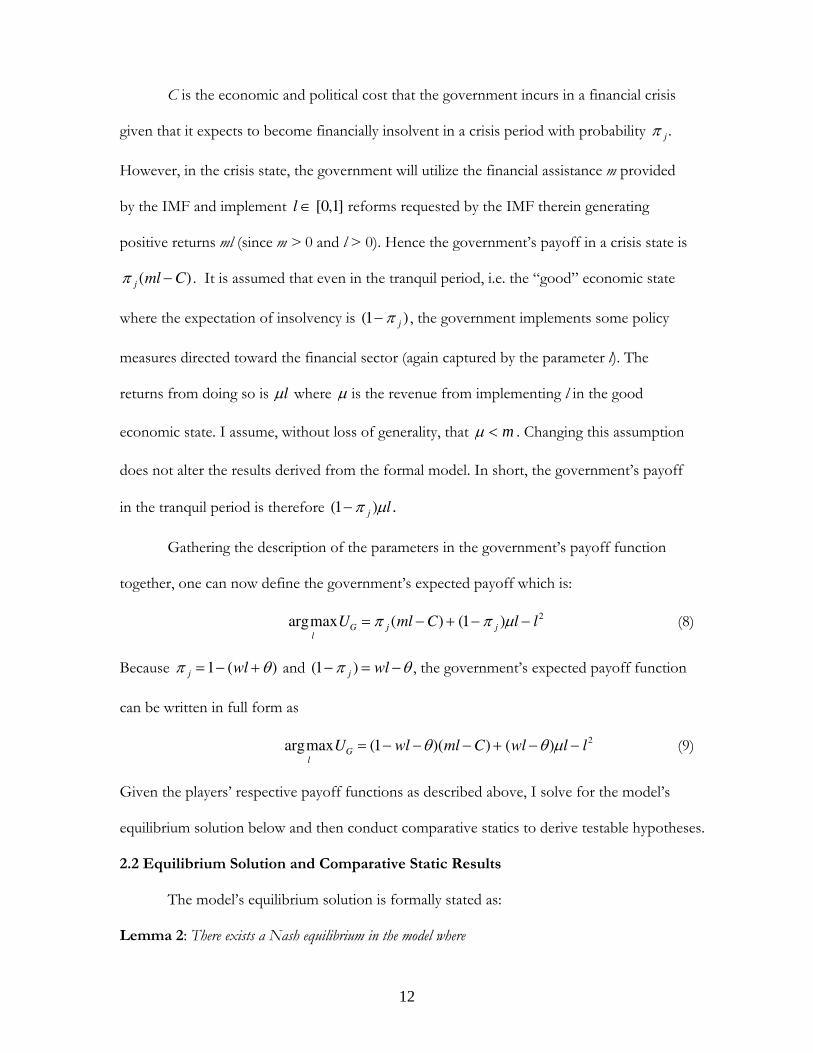
C is the economic and political cost that the government incurs in a financial crisis

given that it expects to become financially insolvent in a crisis period with probability π j .

However, in the crisis state, the government will utilize the financial assistance m provided

by the IMF and implement l ∈ [0,1] reforms requested by the IMF therein generating

positive returns ml (since m > 0 and l > 0). Hence the government’s payoff in a crisis state is

π j (ml − C) . It is assumed that even in the tranquil period, i.e. the “good” economic state

where the expectation of insolvency is (1− π j ) , the government implements some policy

measures directed toward the financial sector (again captured by the parameter l). The

returns from doing so is μl where μ is the revenue from implementing l in the good

economic state. I assume, without loss of generality, that m<μ . Changing this assumption

does not alter the results derived from the formal model. In short, the government’s payoff

in the tranquil period is therefore (1− π j )μl .

Gathering the description of the parameters in the government’s payoff function

together, one can now define the government’s expected payoff which is:

argmaxl

UG = π j (ml − C) + (1− π j )μl − l2 (8)

Because π j =1− (wl + θ) and (1− π j ) = wl −θ , the government’s expected payoff function

can be written in full form as

argmaxl

UG = (1− wl −θ)(ml − C) + (wl −θ)μl − l2 (9)

Given the players’ respective payoff functions as described above, I solve for the model’s

equilibrium solution below and then conduct comparative statics to derive testable hypotheses.

2.2 Equilibrium Solution and Comparative Static Results

The model’s equilibrium solution is formally stated as:

Lemma 2: There exists a Nash equilibrium in the model where

13

(i) The optimal amount of reform implementation by the government of the financially troubled country after receiving financial assistance m from the IMF is:

))(1(2)(*

vmmmvCl

−−−−+

=μ

μθ (10)

(ii) The threshold value of θ*and s* is given by

)(11

1*

*

tFtst

−−−=

−=

σ

θ (11)

(iii) The IMF’s payoff from providing m* is strictly positive (i.e. β(θ,m*) > 0 ) for all θ ≥ θ* and β(θ,m*) < 0 for all θ < θ*. Proof: See Appendix.

The result in Lemma 2 formally characterizes the Nash solution of the model. The

explicit characterization of *θ and *s in Lemma 2 particularly useful because it provides the

necessary technical benchmark that allows one to formally analyze when *θθ < and *ssi <

and this, in turn, provides hypotheses that can be tested on data. While useful, the result in

lemma 1 does not provide substantive insights per se. Rather, comparative statics conducted

on the Nash solutions in Lemma 1 provide the central substantive result from the model,

which is stated formally as

Proposition 1: If the degree of state intervention in the financial sector is high and increasing, then

(i) Implementation of reforms suggested by the IMF declines in equilibrium, 0*

<∂∂

vl

(ii) For strictly decreasing *l and thus 0lim * →l , 0<θ which implies that macroeconomic fundamentals decline in the short-run and (iii) When 0<θ , it follows that *θθ < and *ssi < . Consequently, from Lemma 1 attacking the financially troubled country’s currency becomes a dominant strategy for currency traders and this will substantially increase the likelihood of a currency crisis. Proof: See Appendix.

Proposition 1 predicts that the greater the extent of state intervention in a financially

troubled country’s financial sector, the more likely it is that the financial assistance provided

14

by the IMF under its short-run stabilization program will lead to a currency crisis. The causal

intuition that explains the claim in Proposition 1 directly follows from the technical results in

parts (i), (ii) and (iii) in the proposition and is briefly discussed below. To begin with, note

that when the extent of state intervention in the financial sector is high, political resistance to

reforms requested by the IMF under its short-run stabilization program will be strong both

within and outside the state. Two reasons explain this claim.

First, it is well known (and well publicized) that the IMF provides financial assistance

under its stabilization program to a financially distressed country –that voluntarily participates

in the stabilization program –on the condition that the country adopts in the short-run three

main financial sector reform measures: (i) limit government-directed credit allocation, (ii)

substantially reduce non-performing loans and non-performing assets by public sector banks

and (iii) increase as well as institutionalize financial disclosure of government-owned banks. It

is not difficult to discern that political actors within the state in countries where state ownership

of the banking sector is extensive will particularly resist the IMF reform measure of reducing

government-directed credit allocation schemes even if the concerned state participates in the

IMF’s stabilization program. This is because political actors in countries with extensive state

intervention in banking are more likely to use government-directed credit allocation as a tool

for providing political patronage to constituents and business groups that support them

politically, which, in turn, helps to maximize their political survival in office. In addition to

political patronage, government sponsored credit allocation is also likely to be used by the state

to provide subsidies and welfare that also benefits the state politically. Since reduction of

government-directed credit allocation will endanger the political survival of politicians as well

as force the government to cut back on its welfare programs that may be politically costly,

both specific politicians and the state in general will either overtly or indirectly resist reduction

of government-directed credit allocation.

15

Second, in countries where government intervention in the financial sector is high,

actors outside the state – including representatives from public sector banks and industry

groups—will actively resist the IMF’s financial reform measure that calls for substantial

reduction of non-performing loans and financial assets. Public sector banks will resist a

substantial cut-back on non-performing loans as this may lead to a serious erosion of their

client-base. Industry groups, on the other hand, that benefit from non-performing loans –

which, in effect, provides them with free capital – will also exert political pressure on the

government to not formally implement a reduction in non-performing loans and assets. The

combined political resistance of actors within and outside the state to IMF financial sector

reforms will thus provide political incentives to governments in countries where state

intervention in the financial sector is high to resist cutting back on NP loans. This will

consequently weaken implementation of reform measures in such countries as demonstrated

formally by the comparative static result 0* <∂∂ vl in part (i).

Incomplete or weak implementation of financial sector reform measures suggested

by the IMF as part of its stabilization program will have two immediate effects. First, the

IMF’s financial assistance to a country where government ownership and intervention in the

financial sector is high will engender a serious moral hazard problem. In particular, it is

plausible that IMF loans may be (mis)used in countries with extensive state involvement in

the financial sector to postpone serious financial sector reform for purposes of political

expediency and to protect inefficient public sector banks (with a high percentage of NPAs)

rather than for carrying out the intended reform. Second, if IMF financial packages under its

stabilization program indeed leads ton the moral hazard problem described above, then the

financially troubled country will lack the necessary financial resources to restore its

16

macroeconomic fundamentals and this will lead to a decline in the fundamentals as shown

by the comparative static in part (ii) 0lim * →l , 0<θ .

The model predicts that a decline in θ (that is, 0<θ ) in cases where the IMF

provides conditional financial assistance via its stabilization program has two deleterious

consequences. For one, traders in international capital markets will seriously doubt the

credibility of the financially troubled country’s commitment to carry out IMF-requested

financial sector reforms when the country participates in the stabilization program. Thus,

notwithstanding the financially distressed country’s participation in the stabilization program,

currency traders will rationally expect the country’s fundamentals to fall below the threshold

value of *θ , therein resulting in *θθ < . Second, when the credibility of the participating

country’s commitment to implementing IMF reform measures falters thus leading to

*θθ < , traders also become more uncertain ex ante about the future state of θ . Indeed,

because of higher uncertainty, their realized signal becomes more “noisy” and thus falls

below the threshold *s , i.e. *ssi < (this is proved formally in the proof of proposition 1 in

the appendix). As stated in Lemma 1, when *θθ < and *ssi < , traders find it profitable to

attack the currency of the financially troubled country. And once speculative attacks on the

currency begin, it generates self-fulfilling expectations that not only leads to more speculative

attacks but eventually to a currency collapse.

Put together, the preceding discussion leads to the following hypothesis that is

carefully tested in the next section:

Hypothesis 1: IMF stabilization programs will increase the likelihood of currency crises in financially troubled countries only if the degree of state intervention in the financial sector in countries that borrow from the IMF under the latter’s stabilization program is high. In contrast to the prediction in hypothesis 1, it is not too difficult to discern that IMF

stabilization programs will have the desired effect of decreasing the likelihood of currency

17

crises in financially troubled countries –participating in the program – where the extent of

state intervention in the financial sector is low and decreasing. Two reasons derived from the

model explain this claim. First, participating countries with lower levels of institutionalized

government intervention in the economy are more likely to be characterized by lower

political resistance to financial sector reforms suggested. Such countries that borrow from

the IMF will therefore be in a position to commit more strongly to the reforms requested by

the IMF under its stabilization program. As a result, currency traders will believe that

macroeconomic fundamentals will improve such that *θθ > and will be less uncertain about

the future state of θ therein implying that *ssi > . When *θθ > and *ssi > the incentives

for speculators to engage in a speculative attack against the country’s currency reduced

dramatically and this prevents a currency crisis. More formally,

Corollary 1: For increasing *l (resulting from lower v), 0>θ which leads to *θθ > and *ssi > and IMF stabilization programs thus have a negative effect on the likelihood of a currency crisis. I now turn to test hypothesis 1 in the next section. 3. Statistical Methodology:

3.1 The Spatial Autoregressive Error (SAE) Bivariate Probit Model

In principle, one can use a standard discrete-choice model to test the prediction that

IMF stabilization programs increase the likelihood of a currency crisis when the degree of

state intervention in the financial sector is in financially troubled countries that turn to the

IMF for financial help. Estimating a standard discrete choice model, however, ignores two

methodological problems that confront a researcher testing the impact of IMF stabilization

programs on the likelihood of currency crises. First, there is a sample selection problem

since the participation of countries in IMF stabilization programs is non-random and this

may bias the effect of IMF programs on the likelihood of currency crises. In fact, although

the model presented earlier primarily focuses on when IMF programs prevent currency

18

crashes, it also suggests that only particular countries –in this case, financially troubled

countries with balance of payments and debt problems – voluntarily select into a IMF

stabilization program. That is, my model also provides some explanatory variables that

account for when countries participate in IMF stabilization programs and this should be

incorporated when estimating the impact of IMF stabilization programs on currency crises.

Second, diagnostic tests, specifically the Moran I statistic, on my data reveals that

there is some degree of spatial dependence in the data associated with the occurrence of

currency crises and the participation of countries in IMF stabilization programs. This is not

surprising given that financial contagion exists in the international financial system and that

this can lead to the spread of currency crises and/or engender financial problems across

countries in a region severe enough to encourage these countries to turn to the IMF for

financial help. Hence, while I do not suggest theoretically that spatial dependence is the key

causal variable in my study –clearly governments neither strategically “adopt” a currency

crisis nor participate in IMF stabilization programs because other neighboring countries are

doing so – one needs to explicitly account for spatially autocorrelated disturbances in the

data since it may be a “nuisance” that may bias key parameters of interest.

To account for both sample selection and spatially autocorrelated disturbances –when

participation in IMF stabilization programs and the likelihood of a currency crisis are both

discrete choice processes—I estimate a bivariate probit model with spatial autoregressive

errors (SAE) in both the selection and outcome equations. The spatial autoregressive error

bivariate probit model (hereafter, SAE bivariate probit model), specifies spatially

autocorrelated disturbances (after dropping subscript t for time for notational convenience):

∑≠

+=+′+=ij

ijijiiii ucuuxy 1111110*1 , εδαα (12)

19

∑≠

+=+′+=ij

ijijiiii ucuuxy 2222120*2 , εγββ (13)

where *1iy and *

2iy are latent variables with 1*1 =iy if 0*

1 >iy and 01 =iy otherwise, and 1*2 =iy if

0*2 >iy and 02 =iy otherwise. In the SAE bivariate probit model, equation 11 (i.e. *

1iy ) is the

selection equation that accounts for participation of countries in IMF’s stabilization programs.

Equation (12), namely *2iy , is the outcome equation that accounts for the likelihood of a

currency crisis where *2iy is a currency crisis that occurs in a particular country-year.

The correlation between the residuals iu1 and iu2 is given by ρ , which is standard

in bivariate probit models.5 Note that each of these two equations (11 and 12) exhibit spatial

dependence in their respective error term, as iu1 and iu2 depend on the other ju1 and

ju2 through their location in space, as given by the spatial weights ijc and the spatial

autoregressive parameters δ and γ . I briefly discuss the operationalization of the spatial

weights in (11) and (12) below. At this stage, observe that the errors i1ε and i2ε in (11) and

(12) are iid ),( ∑0N .6 Hence, the SAE bivriate probit model can be written conveniently as

jj

ijii wxy 11

110*1 εαα ∑+′+= (14)

jj

ijii wxy 22

120*2 εββ ∑+′+= (15)

5 ρ is the correlation among the residuals where ⎟⎟

⎠

⎞⎜⎜⎝

⎛⎟⎟⎠

⎞⎜⎜⎝

⎛⎟⎠⎞

⎜⎝⎛

⎟⎟⎠

⎞⎜⎜⎝

⎛1

100~

2

1

ρρ

Nuu

i

i

6 ⎟⎟⎠

⎞⎜⎜⎝

⎛=∑ 2

212

1221

σσσσ

20

where the weights 1ijw and 2

ijw are the (i,j) elements of the inverse matrices 1)1( −− Cδ and

1)1( −− Cγ , respectively, with C the matrix of spatial weights ijc .7

Numerous weighting schemes can be used to operationalize ijw in spatial models. For

e.g., in a linear spatial regression model, Simmons and Elkins (2004: 178) use directed trade-

flow shares of country j in country i’s total for ijw , while Franzese and Hays (2006: 174) code

1=ijw for countries i and j that share a border and 0=ijw for countries that do not. Since I

focus on accounting for spatial autocorrelated disturbances that are more of nuisance in the

data, I use a geographic measure of spatial contiguity that is operationalized as the inverse

distance between states i and j, where ijij dw 1= . As the distance between states i and j

increases (decreases), ijw increases (decreases), thus giving less (more) spatial weight to the

state pair when ji ≠ . While there is no consensus on how distance between cross-sectional

units should be measured, I follow Busch and Reinhardt (2006) and consider the distance

between population centers of countries. The results reported below remain robust when

other measures of spatial contiguity including inverse distance squared, trade-flow shares and

whether or not states share a border.

The technique used to estimate the SAE bivariate probit model is described more

formally in the appendix. Given that SAE engenders a non-spherical VCV matrix that leads to

inconsistent estimates, I propose in the appendix a GMM estimator that also takes into

account heteroskedasticity induced by the SAE process. Specifically, I use Pinske and Slade’s

(1998) estimation technique, which not only provides consistent estimates of all parameters

including the SAE parameter, but also allows one to use the GMM framework for estimation.

3.1 Data and Dependent Variable

7 Both sets of weights 1

ijw and 2ijw depend upon the unknown parameters δ and γ .

21

To test the prediction in hypothesis 1, I put together a time-series-cross-sectional

(TSCS) dataset of 82 countries over the period 1974 to 2002. These countries are listed in

Table 1. I include countries that both did and did not experience a severe currency

crisis/speculative attack during the 1974-2002 sample period. Doing so allows one to make

inferences about the conditions distinguishing countries encountering crises and others

managing to avoid crises. And this, in turn, helps to effectively evaluate the effect of IMF

stabilization programs on the incidence of currency crises in my sample.

<<Insert Table 1 about here>>

Unlike existing empirical studies on the incidence of currency crises in which the

sample is restricted to few countries or years, a key advantage of my sample is its

comprehensiveness with respect to the number of countries and the years in which these

countries are observed. Indeed, the comprehensiveness of my sample provides an opportunity

to make much more generalizable claims about the conditions under which IMF stabilization

programs prevent currency crashes if my hypothesis is supported by the empirical evidence.

That said, the sample used here only starts from 1974 and not earlier primarily because the lack

of data on some critical economic and political control variables (described below) for many

developing countries prevented one from extending the temporal range of the sample.

Recall that the dependent variable in the outcome equation of the bivariate probit

model is the dichotomous variable Currency Crisis. To operationalize this variable, I first

identified currency crises in the data by constructing a measure of monthly exchange rate

pressure and date each by the year in which it occurs. Specifically, currency crises are defined

as “large” changes in a monthly index of currency pressure, measured as a weighted average

of monthly real exchange rate changes and monthly (percent) reserve losses.8 Following

8 Real exchange rate changes are defined in terms of the trade-weighted sum of bilateral real exchange rates against the U.S. dollar, the German mark, and the Japanese yen, where the trade-

22

convention (e.g. Kaminsky and Reinhart, 1999), the weights attached to the exchange rate

and reservation components of the currency pressure index are inversely related to the

variance of changes of each component over the sample for each country. The exchange rate

data is drawn from Reinhart and Rogoff (2004), while the data for reserves is taken from the

IMF’s (2004) International Financial Statistics CD-Rom.

The measure described above presumes that any nominal currency changes

associated with the exchange rate pressure should affect the purchasing power of the

domestic currency, i.e. result in a change in the real exchange rate. This condition excludes

some large depreciations that occur during high inflation episodes, but it avoids screening

out sizable depreciation events in more moderate inflation periods for countries that have

occasionally experienced periods of hyperinflation and extreme devaluation. Large changes

in exchange rate pressure are defined as changes in the pressure index that exceed the mean

plus 2 times the country-specific standard deviation, provided that it also exceeds 5 percent.9

The first condition insures that any large (real) depreciation is counted as a currency crisis,

while the second condition attempts to screen out changes that are insufficiently large in an

economic sense relative to the country-specific monthly change of the exchange rate.

For each country-year in the sample, I construct a binary measure of currency crises,

as defined above where 1 =Currency Crisis and 0 = No currency crisis. A currency crisis is

deemed to have occurred for a given year if the change in currency pressure for any month

of that year satisfies the criteria described above (i.e. two standard deviations above the mean

weights are based on the average of bilateral trade with the United States, the European Union, and Japan in 1980 and 1990 (taken from the IMF’s (2004) Direction of Trade Statistics). Extant measures of currency crises in empirical studies by Kaminsky, Lizondo, and Reinhart (1998) and Kaminsky and Reinhart (1999) define the currency pressure measure in terms of the bilateral exchange rate against a single foreign currency. By defining the effective rate in terms of the three major nations likely to be main trading partners of most countries, the approach I use provides a broader measure than these other studies and is computationally easier to construct than a multilateral exchange rate measure defined in terms of all of a country’s trading partners. 9 The results reported below remain robust for different cut-off points including 3 and 4 percent.

23

as well as greater than five percent in magnitude). To reduce the chances of capturing the

continuation of the same currency crisis episode, I impose windows on the data. In

particular, after identifying each “large” monthly change in currency pressure, I treat any

large changes in the following 24-month window as part of the same currency episode and

skip the years of that change before continuing the identification of new crises. All the

currency crises in the data and the country-years in which they occurred are listed in Table 2.

<<Insert Table 2 about here>>

In addition to Currency Crisis, one also needs to develop a dichotomous measure for

IMF Stabilization Program, which is the dependent variable in the selection equation of the SAE

bivariate probit model. The dummy IMF Stabilization Program (labeled as IMF Program for

convenience) is equal to 1 for countries that voluntarily participate in the IMF’s stabilization

program when they encounter balance-of-payments problems and thus obtain IMF funds that

are specifically designed meet to short-run balance-of-payments objectives. Because the

dummy IMF Program is also an independent variable in the outcome equation of the SAE

bivariate probit model, I describe in more detail how this variable is operationalized.

3.2 Independent and Control Variables

To test the prediction in hypothesis 1, we need two key independent variables in the

outcome equation for the SAE bivariate probit model. As mentioned above, the first

independent variable is the dummy IMF Program that is coded as 1 when the IMF provides

funds to countries – that voluntarily opt for IMF stabilization programs – in order to (i)

assist them in dealing with the effects of externally generated and temporary export

shortfalls, (ii) to provide financial assistance for exceptional balance-of-payments difficulties,

(iii) to increases reserves and (iv) finally to increase confidence in financial markets.

Financing by the IMF under its short-run stabilization program almost always includes two

conditions: (i) financial sector reforms including reduction of government-directed credit

24

allocation and non-performing loans and (ii) institutionalizing financial disclosure. Note that

IMF short-run stabilization programs do not include programs for long-term economic

reform and structural adjustment. Following the criterion described, six types of IMF

funding are provided under its stabilization program: (1) Standby Arrangements (SBA), (2)

Contingency funding facility (CFF), (3) Buffer Stock funding facility (BSFF), (4) Currency

Stabilization funds (CSF), (5) Supplementary Reserve Facility (SRF) and the (6) Extended

Fund Facility (EFF). Therefore, the dummy IMF program is coded as 1 when the IMF

provides either one or some combination of the six types of funds mentioned above to

financially distressed countries that opt to participate in its stabilization program. Among the

six types of funds mentioned above, the EFF has been used in some (few) cases for

financing structural adjustment in low-income developing countries. Hence, I estimate

additional statistical models where the dummy IMF program excludes EFF but includes the

remaining type of IMF funding facilities. Finally, it should be noted that fund facilities such

as the Structural Adjustment Fund (SAF) and the Poverty Reduction and Growth Facility

(PRGF) are not included in the IMF program dummy as these funds are used only for long-

run structural adjustment. Data for IMF program is drawn from the IMF’s (2004) Review of

Fund Facilities and Hutchison (2001).

The second independent variable is the degree of state intervention in the financial

sector of each country. Note that this does not imply financial depth and sophistication of

credit markets within countries. Rather, it refers to the extent to which state-owned financial

institutions plays a role in financial intermediation and providing financial services. I use two

measures to operationalize this variable. The first measure is the ratio of state owned

commercial banks credit to GDP (labeled as State Credit/GDP).10 The second measure is the

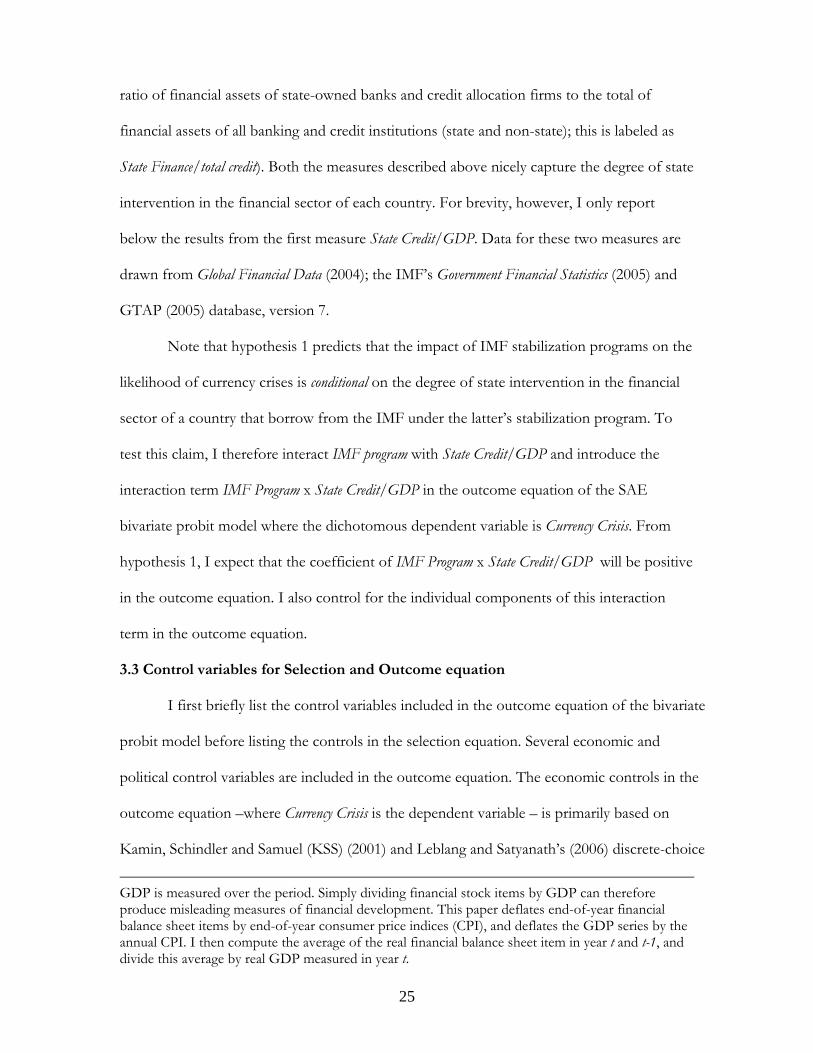
10 Unlike most studies, I carefully deflate those financial intermediary statistics, which are expressed as a ratio to GDP. Specifically, financial stock items are measured at the end of the period, while

25

ratio of financial assets of state-owned banks and credit allocation firms to the total of

financial assets of all banking and credit institutions (state and non-state); this is labeled as

State Finance/total credit). Both the measures described above nicely capture the degree of state

intervention in the financial sector of each country. For brevity, however, I only report

below the results from the first measure State Credit/GDP. Data for these two measures are

drawn from Global Financial Data (2004); the IMF’s Government Financial Statistics (2005) and

GTAP (2005) database, version 7.

Note that hypothesis 1 predicts that the impact of IMF stabilization programs on the

likelihood of currency crises is conditional on the degree of state intervention in the financial

sector of a country that borrow from the IMF under the latter’s stabilization program. To

test this claim, I therefore interact IMF program with State Credit/GDP and introduce the

interaction term IMF Program x State Credit/GDP in the outcome equation of the SAE

bivariate probit model where the dichotomous dependent variable is Currency Crisis. From

hypothesis 1, I expect that the coefficient of IMF Program x State Credit/GDP will be positive

in the outcome equation. I also control for the individual components of this interaction

term in the outcome equation.

3.3 Control variables for Selection and Outcome equation

I first briefly list the control variables included in the outcome equation of the bivariate

probit model before listing the controls in the selection equation. Several economic and

political control variables are included in the outcome equation. The economic controls in the

outcome equation –where Currency Crisis is the dependent variable – is primarily based on

Kamin, Schindler and Samuel (KSS) (2001) and Leblang and Satyanath’s (2006) discrete-choice

GDP is measured over the period. Simply dividing financial stock items by GDP can therefore produce misleading measures of financial development. This paper deflates end-of-year financial balance sheet items by end-of-year consumer price indices (CPI), and deflates the GDP series by the annual CPI. I then compute the average of the real financial balance sheet item in year t and t-1, and divide this average by real GDP measured in year t.

26

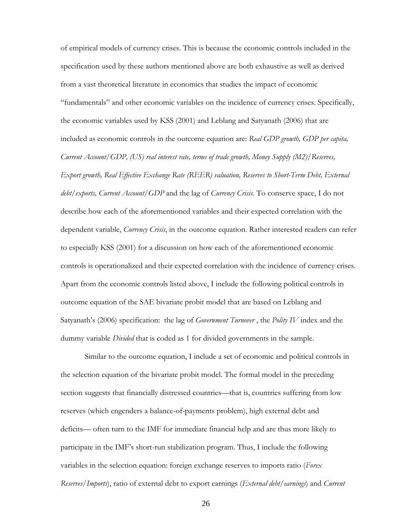
of empirical models of currency crises. This is because the economic controls included in the

specification used by these authors mentioned above are both exhaustive as well as derived

from a vast theoretical literature in economics that studies the impact of economic

“fundamentals” and other economic variables on the incidence of currency crises. Specifically,

the economic variables used by KSS (2001) and Leblang and Satyanath (2006) that are

included as economic controls in the outcome equation are: Real GDP growth, GDP per capita,

Current Account/GDP, (US) real interest rate, terms of trade growth, Money Supply (M2)/Reserves,

Export growth, Real Effective Exchange Rate (REER) valuation, Reserves to Short-Term Debt, External

debt/exports, Current Account/GDP and the lag of Currency Crisis. To conserve space, I do not

describe how each of the aforementioned variables and their expected correlation with the

dependent variable, Currency Crisis, in the outcome equation. Rather interested readers can refer

to especially KSS (2001) for a discussion on how each of the aforementioned economic

controls is operationalized and their expected correlation with the incidence of currency crises.

Apart from the economic controls listed above, I include the following political controls in

outcome equation of the SAE bivariate probit model that are based on Leblang and

Satyanath’s (2006) specification: the lag of Government Turnover , the Polity IV index and the

dummy variable Divided that is coded as 1 for divided governments in the sample.

Similar to the outcome equation, I include a set of economic and political controls in

the selection equation of the bivariate probit model. The formal model in the preceding

section suggests that financially distressed countries—that is, countries suffering from low

reserves (which engenders a balance-of-payments problem), high external debt and

deficits— often turn to the IMF for immediate financial help and are thus more likely to

participate in the IMF’s short-run stabilization program. Thus, I include the following

variables in the selection equation: foreign exchange reserves to imports ratio (Forex

Reserves/Imports), ratio of external debt to export earnings (External debt/earnings) and Current

27

Account Balance as a percentage of GDP. Extant studies suggest that countries with “bad”

economic fundamentals including high inflation, low GDP growth, low GDP per capita, low

levels of domestic investment and higher real exchange rate volatility are more likely to

participate in IMF short-run stabilization programs. Therefore, I also control for the

following variables in the selection equation: GDP per capita, Lag of Inflation, Lag of GDP per

capita growth, Real Effective Exchange Rate (REER) valuation, and Investment as a percentage of

GDP. From recent episodes of currency crises in especially Asia in the 1990s, we also know

that some countries participate in short-run stabilization programs only after a currency crisis

has occurred. A one-period lag of the dummy Currency Crisis is included in the selection

equation to account for this phenomenon. In addition to economic variables, the selection

equation also contains some political controls (i) Veto Players, which is drawn from the Checks

variable in the World Bank’s DPI (Beck et al 2003) and (ii) the dummy variable Latin America

for countries from this region since a fairly large and disproportionate number of Latin

American countries have participated in the IMF’s stabilization programs in the past.

4. Findings and Analyses

The results from the outcome equation of the estimated bivariate probit models are

reported in models 1 to 3 in Table 3, while the estimates from the selection equation of

models 1,2 and 3 are reported in table 4. Because I am primarily interested in the effect of

IMF Program x State Credit/GDP on Currency Crisis –which essentially tests the key theoretical

prediction from the formal model—I focus below on analyzing the results from the

outcome equation and then briefly discuss the results from the selection equation.

<<Insert Table 3 about here>>

The coefficient of IMF Program x State Credit/GDP is positive and highly significant

at the 1% level in the outcome equation of the SAE bivariate probit model for the global

sample. This result statistically corroborates the prediction in hypothesis 1 from the formal

28

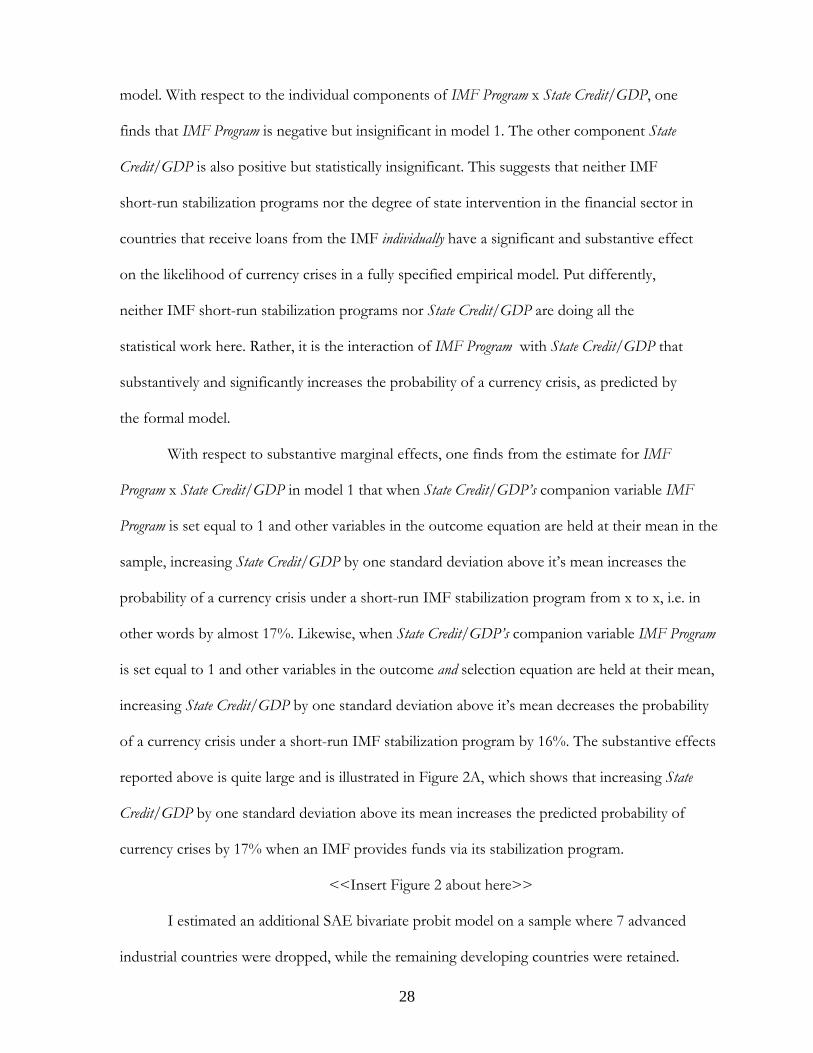
model. With respect to the individual components of IMF Program x State Credit/GDP, one

finds that IMF Program is negative but insignificant in model 1. The other component State

Credit/GDP is also positive but statistically insignificant. This suggests that neither IMF

short-run stabilization programs nor the degree of state intervention in the financial sector in

countries that receive loans from the IMF individually have a significant and substantive effect

on the likelihood of currency crises in a fully specified empirical model. Put differently,

neither IMF short-run stabilization programs nor State Credit/GDP are doing all the

statistical work here. Rather, it is the interaction of IMF Program with State Credit/GDP that

substantively and significantly increases the probability of a currency crisis, as predicted by

the formal model.

With respect to substantive marginal effects, one finds from the estimate for IMF

Program x State Credit/GDP in model 1 that when State Credit/GDP’s companion variable IMF

Program is set equal to 1 and other variables in the outcome equation are held at their mean in the

sample, increasing State Credit/GDP by one standard deviation above it’s mean increases the

probability of a currency crisis under a short-run IMF stabilization program from x to x, i.e. in

other words by almost 17%. Likewise, when State Credit/GDP’s companion variable IMF Program

is set equal to 1 and other variables in the outcome and selection equation are held at their mean,

increasing State Credit/GDP by one standard deviation above it’s mean decreases the probability

of a currency crisis under a short-run IMF stabilization program by 16%. The substantive effects

reported above is quite large and is illustrated in Figure 2A, which shows that increasing State

Credit/GDP by one standard deviation above its mean increases the predicted probability of

currency crises by 17% when an IMF provides funds via its stabilization program.

<<Insert Figure 2 about here>>

I estimated an additional SAE bivariate probit model on a sample where 7 advanced

industrial countries were dropped, while the remaining developing countries were retained.

29

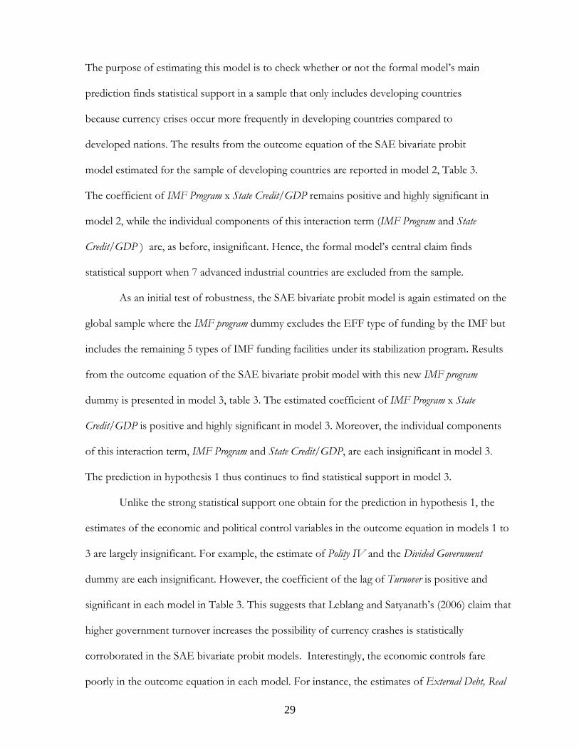
The purpose of estimating this model is to check whether or not the formal model’s main

prediction finds statistical support in a sample that only includes developing countries

because currency crises occur more frequently in developing countries compared to

developed nations. The results from the outcome equation of the SAE bivariate probit

model estimated for the sample of developing countries are reported in model 2, Table 3.

The coefficient of IMF Program x State Credit/GDP remains positive and highly significant in

model 2, while the individual components of this interaction term (IMF Program and State

Credit/GDP ) are, as before, insignificant. Hence, the formal model’s central claim finds

statistical support when 7 advanced industrial countries are excluded from the sample.

As an initial test of robustness, the SAE bivariate probit model is again estimated on the

global sample where the IMF program dummy excludes the EFF type of funding by the IMF but

includes the remaining 5 types of IMF funding facilities under its stabilization program. Results

from the outcome equation of the SAE bivariate probit model with this new IMF program

dummy is presented in model 3, table 3. The estimated coefficient of IMF Program x State

Credit/GDP is positive and highly significant in model 3. Moreover, the individual components

of this interaction term, IMF Program and State Credit/GDP, are each insignificant in model 3.

The prediction in hypothesis 1 thus continues to find statistical support in model 3.

Unlike the strong statistical support one obtain for the prediction in hypothesis 1, the

estimates of the economic and political control variables in the outcome equation in models 1 to

3 are largely insignificant. For example, the estimate of Polity IV and the Divided Government

dummy are each insignificant. However, the coefficient of the lag of Turnover is positive and

significant in each model in Table 3. This suggests that Leblang and Satyanath’s (2006) claim that

higher government turnover increases the possibility of currency crashes is statistically

corroborated in the SAE bivariate probit models. Interestingly, the economic controls fare

poorly in the outcome equation in each model. For instance, the estimates of External Debt, Real

30

Effective Exchange Rate (REER) Valuation, Reserves to Short-Term Debt, Export Growth, Current

Account/GDP and Real Interest Rate are each insignificant in every model. However, Money Supply

(M2)/Reserves and Terms of Trade Growth have the predicted sign and are significant.

Turning to the estimates of the selection equation of models 1, 2 and 3 –that are

reported in Table 4 -- we find a familiar story in that most economic controls are for the most

part statistically insignificant. For example, the estimate of the lag of Inflation, the lag of GDP per

capita growth, Real Effective Exchange Rate Valuation and Investment (as a % of GDP) is statistically

insignificant in the selection equation of each model. However, Forex Reserves/Imports is positive

and highly significant in the selection equation of all the models. The political variable in the

selection equation Veto Players is unfortunately insignificant in the estimated models.

The estimate of the SAE parameter δ is positive and highly significant in the

outcome equation of all the SAE bivariate probit models, while the estimate of the SAE

parameter γ is particularly weakly significant. The significance of δ in the outcome equation

is particularly because it indicates that accounting for spatial effects – that arguably results

from financial contagion -- in the currency crisis outcome equation is critical when

estimating the effect of other parameters on the likelihood of currency crises in order to

avoid biased and inconsistent parameter estimates. Furthermore, the estimate of ρ is

significant in the outcome equation as well, which clearly indicates the selection issues in the

data that needs to be accounted for as well in the estimation process.

4.1 Robustness Tests and Diagnostics

To check the econometric validity and consistency of the results reported earlier, I

conducted a three main robustness tests and a series of diagnostic checks. First, I added two

control variables to the outcome equation of the baseline SAE bivariate probit specification

in model 1and then re-estimated the model, including the selection and the augmented

31

outcome equation. The two additional control variables in the outcome equation are Veto

Players and Number of Past Currency Crises. The Veto Players variable is added to the outcome

equation since Macintyre (2002) suggests that higher number of veto players in government

impedes adjustment to economic shocks and this increases the likelihood of currency

crashes. Likewise, I control for Number of Past Currency Crises since it is plausible that

countries that have suffered from several incidents of currency crises in the past are more

vulnerable to currency crashes. In model 4, Table 5 I report the results from the outcome

equation of the SAE bivariate probit model that includes the two additional controls

mentioned above (the selection equation of this model is not reported to conserve space).

Observe that the estimate of IMF Program x State Credit/GDP is positive and

significant at the 1% level n the outcome equation reported in model 4 while IMF Program

and State Credit/GDP are individually insignificant in this specification. These results are

consistent with the estimates reported earlier in Table 3. Interestingly, Veto Players is

statistically insignificant in model 4, while Number of Past Currency Crises is significant.

Second, I check the robustness of the results reported earlier on two alternative

measures of the dependent variable in the outcome equation of the bivariate probit model,

Currency Crisis. This is done in order to check that the estimates obtained so far are not

driven merely by the operationalization of the dichotomous measure of Currency Crisis in this

paper (as described earlier) even though this measure is widely used in extant studies. The

two alternative measures of the dependent variables that are used for the robustness tests are

drawn from Kamin, Schindler and Samuel (2001) and Bussiere and Fratzscher (2002). Kamin

et al (2001) code a currency crisis as occurring when the index of exchange market pressure

(a weighted average of changes in the real exchange rate and reserve holdings) exceeds its

average value by 1.75 standard deviations. Using monthly data they identify a crisis as

occurring during a year when any month experiences a crisis. Bussiere and Fratzscher

32

(2002), on the other hand, code a crisis as occurring when the weighted average of the

change in the real effective exchange rate, the change in the interest rate, and the change in

reserves is more than 2 standard deviations away from each country’s average.

Using these two operational definitions of currency crashes, I first operationalize the

Kamin et al (2001) measure of currency crashes (labeled as Crisis (KSS)) based on their

definition given above and then operationalize Bussiere and Fratzscher’s (2002) definition of

currency crises (labeled as Crisis (BF)) in the global sample. After doing so, I separately

estimate two models; in the first model, the dependent variable in the outcome equation is

the Kamin et al (2001) dichotomous measure of currency crashes (Crisis (KSS)) and in the

second model, the dependent variable in the outcome equation is Bussiere and Fratzscher’s

(2002) dichotomous measure Crisis (BF).11 The results from these two bivariate probit

models are reported in models 5 and 6 respectively in Table 5. The estimated coefficient of

the interaction term IMF Program x State Credit/GDP is positive and significant at the 1%

level n the outcome equation in model 5 and 6. Moreover, IMF Program and Credit/GDP are

each individually insignificant in the outcome equation of model 5 and 6. Thus the results

reported earlier remain robust when alternative operational definitions of the dependent

variable, Currency Crisis, are used in the outcome equation.

In addition to the robustness tests, I conducted standard diagnostic checks. First,

diagnostic test indicate that none of the empirical models suffer from multicollinearity.12 Second,

I implemented Gourieroux, Monfort and Trognon’s (1982) score test of the null of serially

uncorrelated errors for each model. The p-values from this score test failed to reject the null of

no serial correlation in each specification, thus suggesting that serial correlation is not a problem

11 The dependent variable in each of these two models is IMF program. 12 Chatterjee, Price and Haidi (1999) suggest that multicollinearity exists if the largest Variance Inflation Factor (VIF) is greater than 10 and the mean VIF is larger than 1. The mean and largest VIF value in each empirical model is substantially lesser than these threshold values. Hence, multicollinearity is not a problem.

33

in the models. Third, as an additional check for specification robustness, I added the following

variables to each model: Nominal Interest Rate and the dummy Capital Controls. Inclusion of these

variables did not substantively or significantly alter the results reported above.

5. Conclusion

Why do IMF stabilization programs fail to prevent currency crashes in some

financially distressed countries that voluntarily participate in these stabilization programs but

not other financially troubled countries? The simple model of speculative trading

constructed in this paper suggests that the IMF’s ability (or inability) to prevent currency

crashes via its stabilization program crucially depends on the degree of institutionalized state

intervention in the financial sector of financially distressed countries that participate in the

IMF’s stabilization program. More specifically, the greater (lower) the extent of

institutionalized state intervention in the financial sector of a financially troubled country

that turns to the IMF for help, the higher (lesser) the likelihood that the IMF stabilization

program will fail to prevent a currency crisis in that country. Results from several spatial

bivariate probit models that accounts for both selection bias and spatial dependence in the

data provide strong statistical support for the model’s key theoretical prediction.

The research presented here has important implications. First, the rapid increase in the

volume of currencies traded in capital markets ($ 2 trillion dollars were traded daily in 2004) has

especially made developing countries –that are opening their capital markets –vulnerable to

financial problems and currency crashes. These countries are likely to turn to the IMF in the

future to resolve their financial problems. We thus need to explain rigorously and understand

more generally, and not on a case-by-case basis, when IMF stabilization programs may fail or

succeed in preventing currency crises, as done theoretically and empirically in this paper. Second,

many journalists and policy analysts in the recent past claimed that unchecked speculation by

rapacious and greedy currency traders (i.e. Soros) and “crony capitalism” caused or exacerbated

34

the currency crises of the 1990s. This paper suggests that it is neither crony capitalism nor

speculation by traders but rather the politics surrounding financial sector reform –which is

influenced by the degree of institutionalized state intervention in the financial sector – that

provides a fairly cogent for the occurrence of currency crises in financially troubled countries.

Third, as noted earlier, much of extant literature on the impact of the IMF’s role in the

global economy focus on the effect that IMF programs have on growth, inflation and

unemployment but do not analyze the IMF’s role in currency crisis-prevention. This is

unfortunate since the IMF’s main goal is to promote monetary stability and prevent currency

crises. This paper, therefore, fills a large gap in the literature and address variation in the effect

of IMF stabilization programs on preventing currency crises. Fourth, existing policy

prescriptions by policy-analysts and even the Meltzer Commission report (sanctioned by the US

congress) in 2000 primarily focus on institutional reform of the IMF as the panacea for

preventing IMF failures in the future. While the aforementioned policy prescription is not wrong

per se, it overlooks the fact that the IMF’s ability or inability to prevent currency crashes around

the globe critically depends on the domestic politics of financial sector reform in countries that

borrow from the IMF and participate in the IMF’s stabilization program.

The key policy implication that emerges from this study is that the IMF should either

scale back or increase the time span for carrying out financial sector reforms that it requests

from countries participating in its stabilization programs. Giving governments of financially

distressed countries --that have an entrenched political class opposed to financial reforms –

more time to carry out financial sector reforms will allow them to either build a minimal winning

coalition that favors reform or spread the costs of financial reforms across time. This may ease

political opposition against reforms and give the government an opportunity to carry out

financial sector reforms more extensively that will help to promote better macroeconomic

fundamentals. Whether or not this policy prescription is feasible is a matter for future research.

35

Appendix

Proof of Lemma 1: Since each trader’s private signal is conditional onθ , the pdf of is given θ is g,

while its cdf is )|( θisG . Likewise, let the density of θ given is be h and its cdf as )|( isH θ . I

assume, wlog, that g and h are uniformly distributed such that

h(θ | si) =1/2ε if si −ε ≤ θ ≤ si + ε0 otherwise

⎧ ⎨ ⎩

g(si |θ) =1/2ε if θ −ε ≤ si ≤ θ + ε0 otherwise

⎧ ⎨ ⎩

(A1.1)

Let ]1,0[: →ℜp be the proportion of speculators required for a successful speculative attack.

Let )}(),(|{)( θπθδθπ pP ≥≡ be the event of successful attacks with probability 1 where

),( πθδ is the fraction of traders that attack the currency with probability 1. The expected payoff for a

trader is ∫ −=)(

)|()(),(π

θθθP ii tdshrasu . From theorem 1 in Heinemann and Illing (2002) and

Proposition 2.1 (Coresetti et al 2004), if h and g are uniformly distributed, then ),( asu i strictly

decreases in s and θ . Hence, 1)( =sai when θ < θ* and si < s* QED.

Proof of Lemma 2: (i) Differentiating (x) with respect to l and after some algebra,

))(1(2)(*

vmmmvCl

−−−−+

=μ

μθ (A1.2)

(ii) From Fθ* − s*

σ

⎛

⎝ ⎜

⎞

⎠ ⎟ = t (equation 4), one obtains after some simple algebra θ* = s* + σF −1(t) ;

substituting this expression in equation 3 in the text leads to θ* =1− F(F −1(t)) =1− t . Substituting

θ* =1− t in θ* = s* + σF −1(t)yields 1− t = s* + σF −1(t) . Solving for s*from this expression

leads to s* =1− t −σF −1(t) .

(iii) Since the IMF optimally sets m*, β(θ,m*) > 0 if fundamentals improve such that θ ≥ θ*. If

θ < θ*, the IMF does not earn returns and pays the cost –bm. Thus β(θ,m*) < 0 for θ < θ* QED.

Proof of Proposition 1: (i) 2

*

)](1(2[)22)(()222(

mmmmvCCmvv

vl

−−−+−+−+−

=∂∂

μμθθμμ

which

after some algebra yields 0)](1(2[

))()((2

2*

<−−

−−+−+=

∂∂

mmmmC

vl

μθμμθμ

since m<μ .

36

(ii) From (A1.2), one can implicitly define θ as )(

))(1(2 *

mvmlmvC

−−−−+

=μ

μθ . Since ]1,0[∈l

and *l strictly decreases for increasing v, it follows that 0lim * →l in this case. Note that for

0lim * →l , 0<−+

=mmvC

μθ since m<μ .

(iii) Because ]1,0[∈θ , it follows that when θ strictly decreases 0lim →θ . When 0lim →θ ,

*θθ < since from lemma 1 01* >−= tθ ]1,0[∈∀t . Likewise, when θ strictly decreases and

0lim →θ , iis σε= which *ssi <⇒ . From the proof of Lemma 1, we know that currency

traders will attack the currency of the troubled country with probability 1 for *θθ < and *ssi < thus leading to a currency crisis QED.

Estimation of Spatial Bivariate Probit Model: Suppose that:

( ) ( )∑=j

ijiu 21211var ωσ (A1.3)

( ) ( )∑=j

ijiu 22222var ωσ (A1.4)

( ) ( )∑=j

ijijii uuE ., 22121221 ωωσ (A1.5)

Let { }δααθ ,'1,01 = be the parameters to be estimated in the spatial probit model, and

( )( )i

ii u

x

1

1'10

1 varαα

θψ+

= in the index function of the probit model weighted by the standard deviation

of the residual. The “generalized residuals” of this model are:

( ) ( )[ ]{ } ( )[ ]( )[ ] ( )[ ]{ }.

1~

11

11111 θψθψ

θψφθψθ

ii

iiii yu

Φ−Φ⋅Φ−= (A1.6)

The GMM estimates for 1θ can be obtained as follows:

( ) ( )1'

1,111

minargˆ θθθθ

NNNGMM SMSΘ∈

= (A1.7)

where ( ) ( ) NNNN zuzN

S ,ˆ111

'1 θθ = is a data matrix of regressors plus at least one instrument (to

identify the extra parameter δ , ( )11~ θNu is the vector of generalized residuals with elements as

shown in (A1.6), and NM is a positive definite matrix such that MMp

N → . Pinkse and Slade

(1998) prove that this estimator is consistent and asymptotically normal. From the consistent

37

estimates of 1θ , one can construct the IMR to correct for sample selection bias in the outcome

equation as follows:

[ ] ( )[ ]1'10121

'2012 0 ααββ iiiiii xuuExyyE +−>++=>

( )( )

( )[ ]( )[ ]{ }1

1

1

211

'20 1var

,θψ

θψφββ

i

i

i

iii u

uuEx

−Φ−−

⋅++=

( )( )[ ]

( )[ ]{ }1

1

2121

2112

1'20 1 θψ

θψφ

ωσ

ωωσββ

i

i

jij

jijij

ix−Φ−

−⋅++=

∑

∑

( )( )[ ]

( )[ ]{ }1

1

21

21

1

121

'20 1 θψ

θψφ

ω

ωω

σσ

ββi

i

jij

jijij

ix−Φ−

−⋅⋅++=

∑

∑

Therefore, the selectivity correction implies the following “adjusted” IMR:

( )( )[ ]

( )[ ]{ }1

1

21

21

1 θψθψφ

ω

ωωλ

i

i

jij

jijij

i −Φ−−

⋅≡∑

∑. (A1.8)

Once estimated ( )iλ̂ , the “adjusted” IMR may be included as an additional variable in the outcome

equation, which in turn could be estimated spatial methods for probit models. I use GMM to estimate

simultaneously all parameters of the sample selection model by rewriting it as a sequential estimator

(Newey 1984) composed of the Pinske and Slade (1998) and KP-SAE estimators. Stacking the

corresponding moment conditions leads to ( ) ( ) ( )[ ]''2

'1 ,,,, θθθ NNN zmzszg = ,

{ }γμββδααθ ,,,,, '10

'1,0= with ( ) ( )θθ NNN uzzs 1

'11

~, = , ( )θNu1~ and

( ) [ ] ( )θθ NNNN uzyzm 2'

212~, ⋅= , ( ) ( )γδλμββθ ,ˆ~

1'2022 NNNN xyu −−−= where N denotes the

corresponding matrix of data, we let [ ]( ) NNNNN zzyzz 1

''21

'1

' ,, ⋅= and Nz2 includes the regressors from

the selection and outcome equation respectively with the estimated “adjusted” IMR in the outcome

equation represented as ( )γδλ ,ˆN to make explicit its dependence on both SAE parameters. Let

( ) ( ) ( )( )''2

'1

~,~~ θθθ NNN uuu = ; then the parameters of the SAE sample selection model can be estimated as:

( ) ( )θθθθ

NNNGMM gMg 'minargˆΘ∈

= (A1.9)

where ( ) ( )θθ NNN uzN

g ~1 '= , for a conformable positive definite NM such that MMp

N → .

38

Table 1. Countries Included in the Dataset, 1974-2002 Country Country Argentina Madagascar Bangladesh Malawi Belgium Malaysia Belize Mali Bolivia Malta Botswana Mauritius Brazil Mexico Burundi Morocco Cameroon Mozambique Chile Myanmar Colombia Nepal Costa Rica Nicaragua Cyprus Nigeria Czech republic Pakistan Denmark Panama Dominican Republic Paraguay Ecuador Peru Egypt Philippines El Salvador Poland Equatorial Guinea Sierra Leona Ethiopia Singapore France South Africa Ghana Spain Grenada Sri Lanka Guatemala Swaziland Guinea-Bissau Syria Guyana Sweden Haiti Thailand Honduras Trinidad & Tobago Hong Kong Tunisia Hungary Turkey Italy Uganda India United Kingdom Indonesia United States Italy Uruguay Jamaica Venezuela Jordan Zambia Kenya Zimbabwe Korea Lao P.D. Republic

39

Table 2: Incidence of Currency Crises, 1974-2002 Country Currency Crises Country Currency Crises Argentina 1975,1982, 1989, 2002 Madagascar 1984, 1986, 1991, 1994 Bangladesh 1975 Malawi 1982, 1985, 1992, 1994 Belgium 1992 Belize Malaysia 1986, 1997 Bolivia 1981, 1983, 1988, 1991 Mali 1993 Botswana 1984, 1996 Malta Brazil 1982, 1987, 1990, 1995 Mauritius 1979 Burundi 1976, 1983, 1986,1989,

1997 Mexico 1976, 1982, 1985, 1994

Cameroon 1982, 1984, 1994 Morocco 1983, 1990 Chile 1985 Mozambique 1993, 1995 Colombia 1985 Myanmar 1975, 1977 Costa Rica 1981 Nepal 1975, 1981, 1984, 1991, 1995Cyprus 1976, 1989 Nicaragua 1993 Denmark 1992 Dominican Republic 1985, 1987, 1990 Nigeria 1986, 1989, 1992 Ecuador 1982, 1985, 1988 Pakistan None Egypt 1979, 1989 Panama None El Salvador 1986, 1990 Paraguay 1984, 1986, 1988, 1992 Equatorial Guinea 1991, 1994 Peru 1976, 1979, 1987 Ethiopia 1992 Philippines 1983, 1986, 1997 Fiji 1986 Poland 1997 France 1992 Sierra Leona 1988, 1990, 1997 Ghana 1978, 1983, 1986 Singapore 1975 Grenada 1978 South Africa 1987 Guatemala 1986, 1989 Sri Lanka 1977 Guinea-Bissau 1991, 1996 Spain 1992 Guyana 1987, 1989 Swaziland 1975, 1979, 1982, 1984 Haiti 1977, 1991 Syria 1977, 1982, 1988 Honduras 1990 Thailand 1981, 1984, 1997 Hong Kong 1998 Trinidad & Tobago 1985, 1988, 1993 Hungary 1994, 1997 Tunisia 1993 India 1976, 1991, 1995 Turkey 1978, 1985, 2002 Indonesia 1978, 1983, 1986, 1997 Uganda 1981, 1987, 1989 Italy 1978, 1992 United Kingdom 1992 Jamaica 1978, 1983, 1990 Uruguay 1982 Jordan 1983, 1987, 1989, 1992 Venezuela 1984, 1986, 1989, 1994 Kenya 1975, 1981, 1985, 1993,

1995, 1997 Zambia 1985, 1994

Korea 1980, 1997 Zimbabwe 1982, 1991, 1994, 1997 Lao P.D. Republic 1995

40

Table 3: Results from Outcome Equation of SAE Bivariate Probit Models

IMF program

IMF program

(excluding EFF) Global Developing Global Developing Model 1 Model 2 Model 3 Model 4 GDP per capita -.047***

(.015) -.051** (.027)

-.040*** (.018)

-.037* (.020)

Real GDP Growth .047 (.041)

.040 (.043)

.032 (.044)

.030 (.036)

Current Account/GDP

-.031 (.022)

-.025 (.021)

-.020 (.020)

-.021 (.022)

IMF program -.073 (.082)

-.031 (.040)

-.050 (.046)

-.033 (.037)

IMF program x state credit/gdp .112*** (.036)

.138*** (.044)

.137*** (.055)

.125*** (.040)

State credit/gdp .098 (.077)

.065 (.092)

.023 (.084)

.067 (.119)

(US) Real Interest Rate .027 (.048)

.021 (.020)

.022 (.031)

.021 (.040)

Terms of Trade Growth -.021** (.009)

-.044*** (.020)

-.034** (.017)

-.059* (.035)

M2/Reserves .023*** (.011)

.025*** (.012)

.037** (.018)

.051*** (.020)

Export Growth -.047 (.043)

-.068 (.112)

-.039 (.077)

-.022 (.055)

Reserves/short-term debt .028 (.071)

.030 (.022)

.039 (.041)

.012 (.008)

External debt/exports .01 (.01)

.03 (.02)

.02 (.01)

.04 (.05)

REER valuation .078 (.071)

-.057 (.052)

.064 (.059)

-.095 (.086)

Polity IV -.027 (.023)

-.038 (.073)

-.036 (.032)

-.035 (.037)

Divided Government .06 (.04)

.08 (.09)

.05 (.03)

.08 (.07)

Government Turnover .031* (.019)

.024* (.013)

.033* (0.18)

.051* (.027)

Lagged Currency Crisis .053* (.031)

.040* (.022)

.042* (.023)

.041* (.022)

Constant .551*** (.045)

.672*** (.056)

.447*** (.062)

.424** (.061)

Rho -.112*** (.047)

-.098*** (.032)

-.103*** (.028)

-.125*** (.041)

SAE parameter (γ ) .045** (.020)

.040*** (.017)

.035*** (.011)

.033*** (.012)

Log Likelihood -214.36 -177.23 -182.78 -148.09 N 2174 1889 2174 1889

2χ 29.43 36.25 40.78 51.76 Notes: ***, **, *: 1%, 5% and 10% levels of significance. Numbers in parentheses are robust standard errors.

Coefficient of adjusted IMR ( )iλ̂ not reported to save space.

41

Table 4: Results from Selection Equation of Spatial Bivariate Probit models

IMF program IMF program (excluding EFF)

Global Developing Global Developing selection

equation for Model 1

selection equation for

Model 2

selection equation for

Model 3

selection equation

for Model 4 Investment -.053*

(.031) -.040* (.022)

-.042* (.023)

-.041* (.022)

Forex Reserves/Imports -.047*** (.015)

-.051*** (.019)

-.038*** (.015)

-.031*** (.012)

Lag Inflation .047 (.041)

.040 (.043)

.032 (.044)

.030 (.036)

Trade Openness -.198 (.177)

-.065 (.092)

-.123 (.184)

-.067 (.119)

External debt/export earnings

.031 (.022)

.025 (.021)

.020 (.020)

.021 (.022)

Current Account Balance .073 (.082)

.031 (.040)

.050 (.046)

.033 (.037)

GDP per capita growth -.027 (.048)

-.021 (.020)

-.022 (.031)

-.021 (.040)

Lag Currency Crisis .023*** (.010)

.055*** (.014)

.027** (.011)

.051** (.025)

State credit/gdp .032** (.016)

.059** (.025)

.039** (.018)

.020*** (.006)

GDP per capita -.040 (.043)

-.068 (.112)

-.039 (.077)

-.022 (.055)

REER valuation .028 (.071)

.030 (.022)

.039 (.041)

.012 (.08)

Veto Players .027 (.023)

-.078 (.073)

.036 (.032)

-.035 (.037)

Latin America Dummy .06 (.04)

.08 (.09)

.02 (.01)

.04 (.05)

Constant .721***

(.0077) 0.508*** (.0068)

0.743*** (.0079)

0.605*** (0.083)

SAE parameter (δ ) .021* (.012)

.032* (.020)

.028* (.016)

.022* (.012)

Log Likelihood -412.52 -380.47 -324.65 -315.10 N 2174 1889 2174 1889

2χ 21.154 20.324 19.439 18.259 Notes: ***, **, *: 1%, 5% and 10% levels of significance. Numbers in parentheses are robust standard errors

42

Table 5: Outcome Equation Results from Robustness tests: Global Sample Additional

Controls KSS Measure of Currency Crisis

FS Measure of Currency Crisis

Model 5 Model 6 Model 7 GDP per capita -.025***

(.011) -.031** (.016)

-.028** (.015)

Real GDP Growth .053 (.043)

.065 (.097)

.057 (.067)

Current Account/GDP

-.024 (.028)

-.031 (.030)

-.035 (.034)

IMF program -.047 (.033)

-.038 (.042)

.029 (.075)

IMF program x state credit/gdp .104*** (.041)

.121*** (.038)

.122*** (.043)

State credit/gdp .098 (.077)

.065 (.092)

.023 (.084)

(US) Real Interest Rate .012 (.08)

.023 (.020)

.025 (.016)

Terms of Trade Growth -.029** (.007)

-.020** (.008)

-.024*** (.007)

M2/Reserves .035*** (.011)

.041** (.010)

.046*** (.009)

Export Growth -.050 (.046)

-.054 (.041)

-.042 (.039)

Reserves/short-term debt .059 (.050)

.021 (.019)

.044 (.031)

External debt/exports .008 (.014)

.010 (.011)

.009 (.012)

Polity IV -.035 (.037)

- .021 (.033)

-.026 (.035)

Divided Government .001 (.001)

.002 (.002)

.001 (.003)

Government Turnover .068** (.030)

.051** (.021)

.033*** (.010)

Veto Players .011 (.029)

Number of Prior Crises .021** (.009)

.040* (.012)

.032** (.010)

Constant .339*** (.072)

.290*** (.089)

.316*** (.078)

Rho -.091*** (.030)

-.087*** (.024)

-.093*** (.025)

SAE parameter (γ ) .047*** (.021)

.040** (.020)

.032*** (.011)

Log Likelihood -137.45 -142.26 -170.91 N 2073 2136 2088

2χ 63.87 71.25 81.44 Notes: ***, **, *: 1%, 5% and 10% levels of significance. Numbers in parentheses are robust standard errors.

Coefficient of adjusted IMR ( )iλ̂ not reported to save space.

43

Figure 2A: Marginal Effect of IMF Program x State Credit/GDP on Currency Crisis

0

.2

.4

.6

.8

1

Pr(C)

0 .6Credit/gdp

IMF program=1

Figure 2B: Marginal Effect of IMF Program x Inverse of State Credit/GDP on Currency Crisis

0

.2

.4

.6

.8

1

Pr(C)

0 1.7Inverse of Credit/GDP

IMF program=1

44

Figure 1: Smoothed transition probability of Currency Crisis (S=1) in Thailand 1997-1999

IMF stabilization package 1.0 p11 1-p22 Prob. (S=1) 0 Jan 97 july 97 feb 98 jan 99

45

References

Alesina, Alberto, Nouriel Roubini and Gerald Cohen. 1997. Political Cycles and the Macroeconomy. Cambridge, MA: MIT Press. Alesina, Alberto and Allen Drazen. 1991. Why are Stabilizations Delayed? A Political Economy Model. American Economic Review 81: 1170-1188. Beck, T., G. Clarke, A. Groff, P. Keefer, and P. Walsh. 2003. Database of Political Institutions, Washington DC: World Bank. Berg, Andrew and Carol Pattilllo. 1999a. Are Currency Crises Predictable? A Test. IMF Staff Papers Vol 46, No. 2. Berg, Andrew and Carol Pattilllo. 1999b. Prediciting Currency Crises: The Indicators Approach and an Alternative. Journal of International Money and Finance. 18 (1999): 561-586. Bussiere, Mathieu, and Marcel Fratzscher. 2002. Towards a New Early Warning System of Financial Crises. ECB Working Paper No. 145. (http://www.ecb.int/pub/wp/ecbwp145.pdf) Bussiere, Matthieu and Christian Mulder. 2000. Political Instability and Economic Vulnerability. International Journal of Finance and Economics 5: 309-330. Calvo, Guillermo and Enrique Mendoza. 2000a. “Rational Contagion and the Globalization of Securities Markets,” Journal of International Economics 51:79-113. Calvo, Guillermo and Enrique Mendoza. 2000b. “Capital-Market Crises and Economic Collapse in Emerging Markets: An Information-Frictions Approach,” American Economic Review 90 (May). Corsetti, Giancarlo, Stephen Morris, Amil Dasgupta and Hyun Song Shin. 2004. "Does One Soros Make a Difference? A Theory of Currency Crises with Large and Small Traders," Review of Economic Studies 71: 87-114. Dreher, Axel and Roland Vaubel, 2004a, Do IMF and IBRD cause moral hazard and political business cycles? Evidence from panel data, Open Economies Review 15(1): 5-22 . Eichengreen, Barry, Andrew Rose, and Charles Wyplosz (1995), “Exchange Market Mayhem: The Antecedents and Aftermath of Speculative Attacks,” Economic Policy 21:45-61. Eichengreen, Barry and Andrew Rose. 2003. “Does it Pay to Defend against a Speculative Attack?” in ManagingCurrency Crises in Emerging Markets (edited by Jeffrey Frankel and Michael Dooley, Berkeley: University of California Press. Frankel, Jeffrey A. and Andrew K. Rose. 1996. “Currency Crises in Emerging Markets: An Empirical Treatment.” Journal of International Economics, Vol 41 (November), pp. 351-66. Frieden, Jeffry, Piero Ghezzi, and Ernesto Stein. 2001. “Politics and Exchange Rates: A Cross Country Approach,” in The Currency Game: Exchange Rate Politics in Latin America (eds. Jeffry Frieden and Ernesto Stein). Washington, DC: Johns Hopkins University Press. . Goldstein, Morris, Graciela Kaminski, and Carmen M. Reinhart. 2000. Assessing Financial Vulnerability: An Early Warning System for Emerging Markets. Washington D.C.: Institute for International Economics.

46

Heinemann, Frank and Gerhard Illing. 2002. Speculative Attacks: Unique Equilibrium and Transparency. Journal of International Economics. 58. pp. 429-450. Hutchison, M. 2001. “A cure worse than the disease: Currency Crises and the output costs of IMF-supported Stabilization programs.” Unpublished Ms. EPRU, Denmark. Kamin, Steven M., John Schindler, Shawna Samuel. 2001. The Contribution of Domestic and External Factors to Emerging Market Devaluation Crises. International Finance Discussion Papers 2001/711. (http://www.federalreserve.gov/pubs/ifdp/2001/711/ifdp711.pdf) Kaminski, Graciela, Saul Lizondo, and Carmen M. Reinhart. 1998. Leading Indicators of Currency Crises. IMF Staff Papers Vol 45, No. 1 (March 1998). (www.imf.org) Krugman, Paul. 1979. A Model of Balance of Payments Crises. Journal of Money, Credit, and Banking 11. pp. 311-325. Kumar, Manmohan S., Uma Moorthy, and William Perraudin. 2002. Predicting Emerging Market Currency Crises. Working Paper 02/7. (www.imf.org) Leblang, David and William Bernhard 2001, “The Politics of Speculative Attacks in Industrial Democracies,” International Organization 54:291-324. Leblang, David 2002, “The Political Economy of Speculative Attacks in the Developing World,” International Studies Quarterly 46:69-91. Leblang, David 2003, “To Devalue or to Defend: The Political Economy of Exchange Rate Policy in the Developing World,” International Studies Quarterly 47:533-59. Leblang, David and Shanker Satyanath. 2006. “Institutions, Expectations and Currency Crises,” International Organization Morris, Stephen and Hyun Song Shin. 1998. Unique Equilibrium in a Model of Self Fulfilling Currency Attacks. American Economic Review 88. pp. 587-597. Morris and Shin 2000- Morris, Stephen and Hyun Song Shin. 2000. Rethinking Multiple Equilibria in Macroeconomic Modeling. NBER Macroeconomics Annual 2000, pp139-161. Cambridge: MIT Press. (http://www.econ.yale.edu/~sm326/research.html) Obstfeld, Maurice. 1996. Models of Currency Crisis with Self Fulfilling Features. European Economic Review 40, 1037-1047. Stone, Randall. 2002. Lending Credibility: The International Monetary Fund and the Post-Communist Transition. Princeton: Princeton University Press. Vreeland, James. 2003. The IMF and Economic Development, Cambridge: Cambridge University Press. Vreeland, James. 2005. The International and Domestic Politics of IMF Programs, Yale University, mimeo.