Why do Unemployment Benefits Raise Unemployment Durations?The Role of Borrowing Constraints and Income Effects

Raj Chetty∗

UC-Berkeley and NBER

November 2005

Abstract

It is well known that unemployment benefits raise unemployment durations. Thisresult has traditionally been interpreted as a substitution effect caused by a re-duction in the price of leisure relative to consumption, generating a deadweightburden. This paper questions the validity of this interpretation by showing thatunemployment benefits can also affect durations through a non-distortionary in-come effect for agents who face borrowing constraints. The empirical relevance ofborrowing constraints and income effects is evaluated in two ways. First, I dividehouseholds into groups that are likely to be constrained and unconstrained basedon their asset holdings, mortgage payments, and spouse’s labor force status. Ifind that increases in unemployment benefits have small effects on durations inthe unconstrained groups but large effects in the constrained groups. Second,I find that lump-sum severance payments granted at the time of job loss sig-nificantly increase durations, particularly among households that are likely tobe constrained. These results suggest that temporary benefit programs havesubstantial income effects, challenging the prevailing view that social safety netscreate large efficiency costs.

Keywords: liquidity constraints, consumption smoothing, insurance

∗E-mail: chetty@econ.berkeley.edu. I have benefited from discussions with Alan Auerbach, David Card,Martin Feldstein, Jon Gruber, Jerry Hausman, Caroline Hoxby, Larry Katz, Emmanuel Saez, Adam Szeidl,and numerous seminar participants. Philippe Bouzaglou, David Lee, and Jim Sly provided excellent researchassistance. Funding from the National Science Foundation and NBER is gratefully acknowledged.

1 Introduction

One of the classic empirical results in public finance is that social insurance programs such

as unemployment insurance (UI) reduce labor supply. For example, Moffitt (1985), Meyer

(1990), and others find that a 10% increase in unemployment benefits raises average unem-

ployment durations by 4-8% in the U.S.1 The traditional interpretation of these findings

is that UI induces substitution toward leisure by distorting the relative price of leisure and

consumption, generating a moral hazard efficiency cost. In their recent handbook chapter

on social insurance, Krueger and Meyer (2002) observe that behavioral responses to UI and

other social insurance programs are probably so large because they “lead to short-run varia-

tion in wages with mostly a substitution effect.” Similarly, Gruber (2005) remarks that “UI

has a significant moral hazard cost in terms of subsidizing unproductive leisure.” The logic

underlying these interpretations is presumably that transitory UI benefits are a small part

of lifetime wealth for most individuals, and UI therefore generates only substitution effects

(with negligible income effects).

An important assumption in this logic is that households are able to access lifetime wealth

while unemployed, which requires that they do not face borrowing constraints. However,

recent studies of consumption smoothing give compelling evidence that many unemployed

agents do face binding borrowing constraints. Gruber (1997) finds that increases in UI bene-

fits reduce the consumption drop during unemployment, indicating that agents are unable to

smooth consumption perfectly. Browning and Crossley (2001) and Bloemen and Stancanelli

(2003) provide more direct evidence for the borrowing constraint mechanism by showing that

the UI-consumption link identified by Gruber holds only for the subset of individuals who

report holding few assets at the time of job loss. Nearly half of job losers in the United

States report zero liquid wealth at the time of job loss, suggesting that borrowing constraints

are potentially relevant for a large fraction of the unemployed.

1Atkinson and Micklewright (1990) and Krueger and Meyer (2002) give excellent reviews of this literature.

1

In this paper, I analyze a model where unemployed agents face borrowing constraints,

and show that the effect of UI benefits on durations may largely be due to a non-distortionary

income effect in this environment. To see the intuition, first note that the wealth effects

of UI are indeed small for agents who are able to smooth consumption during unemploy-

ment spells, since UI benefits do not change permanent income very much.2 But when

agents are borrowing constrained, their behavior while unemployed is determined by cash on

hand rather than lifetime resources. UI benefits have a 1-1 effect on relaxing the liquidity

constraint for such individuals, raising their level of consumption while unemployed and po-

tentially making their optimal reservation wage higher or search effort lower. Consequently,

durations can rise simply because agents have more cash on hand, independent of changes

in the relative price of consumption and leisure. Importantly, this income effect is non-

distortionary: It does not arise from a wedge between private and social marginal costs and

therefore does not generate a deadweight burden. A benevolent social planner would not

choose to undo behavioral responses to lump-sum income grants. Hence, once one admits

the possibility of borrowing constraints, it is important to estimate the relative magnitudes

of income and substitution effects caused by unemployment insurance to assess its efficiency

cost.

I use two complementary methods to evaluate the empirical relevance of borrowing con-

straints and income effects. The first method explores the role of constraints in the UI-

duration link by estimating the total effect of UI benefits on durations separately for con-

strained and unconstrained households. The goal of this heterogeneity analysis is to deter-

mine whether it is plausible that income effects are important. For example, if UI benefits

were to affect durations only among unconstrained households, income effects could not be

central. But if the UI-duration link is driven primarily by constrained households, then it

is possible that income effects due to borrowing constraints are relevant.

2For frequent job losers, the income effects of UI may be non-trivial even if they do not face liquidityconstraints. This point is discussed in greater detail in section 2.

2

An obvious difficulty in implementing the heterogeneity analysis is that one cannot di-

rectly observe which households are constrained in the data. To overcome this latent

variable problem, I use several proxies that have been shown to predict constraints in stud-

ies of consumption smoothing. The first is simply a household’s liquid asset holdings (or

assets normalized by prior wages), net of unsecured debt. Households with higher levels of

assets at the time of unemployment are less likely to be constrained than those who have

a smaller buffer stock. The second proxy is whether the individual has a working spouse.

Dual-earner households are more likely to have the resources and credit access necessary to

smooth consumption when one of them loses a job. The third proxy is whether the indi-

vidual has to make a home mortgage payment, which is a relatively rigid commitment that

effectively reduces liquid wealth as well.

I first examine the effect of UI benefits on unemployment exit hazards in each of the

constrained and unconstrained groups nonparametrically. I divide individuals into two

categories: Those in high-UI benefit regimes (state/year pairs with UI benefits above the

sample median) and those in low-UI benefit (below median) regimes. I then plot Kaplan-

Meier survival curves for these two categories and conduct non-parametric tests for differences

in the hazard rate across the two groups. The visual analysis and statistical tests uniformly

show little correlation between UI benefits and hazard rates among the unconstrained groups

(those with more than $1000 in liquid wealth, those with a working spouse, and those without

a mortgage). However, there is a very strong link, both economically and statistically,

between the level of benefits and unemployment exit rates in all the constrained groups.

I then estimate a set of semiparametric Cox hazard models to evaluate the robustness

of these results to controls. The point estimates indicate that a 10% increase in benefits

raises unemployment durations by around 6-8% in the constrained groups, but have little

or no effect in the unconstrained groups. Moreover, the effect of UI on durations becomes

monotonically larger as we examine groups of households that are progressively more likely

to be constrained (e.g., as liquid wealth holdings fall). These results are fully robust to

3

the inclusion of rich controls and other specification checks such as the permission of unob-

served heterogeneity in baseline hazards. In addition, there is no association between UI

benefits and durations in the “control group” of UI-ineligible and non-claiming individuals,

supporting the exogeneity of the UI benefit rates.

These results show that the link between unemployment benefits and durations docu-

mented in prior studies is driven by a subset of the population that is liquidity constrained.

This result requires careful interpretation. Barring additional assumptions, the evidence

does not establish that constraints cause larger responses to UI benefits. It simply shows

that UI benefits have different effects in constrained and unconstrained groups. Whether

these differences arise because of the constraints themselves or because of correlation in

preferences and asset holdings, mortgage commitments, etc. (which are endogenous to pref-

erences) is unclear. What is clear, however, is that the substitution effect for the uncon-

strained group is small, and that the benefit elasticity of durations in the constrained group

is large. These findings are consistent with the hypothesis that an income effect is involved

in the UI-duration link, but do not establish the existence of an income effect by themselves.

This observation motivates the second portion of the empirical analysis, in which I explic-

itly decompose the benefit elasticity of unemployment durations into income and substitution

effects using variation in lump-sum severance payments. To do so, I use a new dataset that

matches survey data collected byMathematica with administrative records on unemployment

durations. Non-parametric tests show that individuals who received a lump-sum severance

payment (worth about $1000 on average) at the time of job loss have substantially lower

unemployment exit hazards, implying that income effects are indeed large. An obvious

concern is that this finding may reflect correlation rather than causality because severance

pay is not randomly allocated. Two pieces of evidence support the causality of severance

pay. First, the estimated effect of severance pay is virtually unchanged with the inclusion

of a large set of controls for demographics, income, job tenure, industry, and occupation in

a Cox model. Second, severance payments have a large positive effect on durations among

4

constrained (low asset) households, but have no effect on durations among unconstrained

households. Since there is no a priori reason to expect a differential effect of severance

pay by asset holdings under the most plausible omitted-variable hypotheses, this evidence

supports the causality of income effects.

Combining the point estimates from the two empirical approaches, a simple calculation

indicates that roughly 70% of the duration elasticity of UI benefits is due to an income

effect. Note that the evidence does not indicate that UI induces no substitution effect:

There is certainly some response to distorted marginal incentives that generates a deadweight

cost.3 The finding that income effects are large in unemployment durations also does

not contradict studies of labor supply behavior which generally find small income effects

relative to substitution effects. As emphasized by Krueger and Meyer (2002) and Chetty

(2003), income and substitution elasticities can be very different for the short-run variation

in wages and income induced by programs such as UI than for the long-run variation in

wages and wealth that determine decisions such as hours worked and retirement ages. The

elasticities need not be the same because long-term labor supply decisions are determined

purely by preferences over wealth and leisure, whereas features such as liquidity constraints

and adjustment costs also affect unemployment durations.

I would like to emphasize two limitations of the present analysis before proceeding. First,

a full welfare analysis of UI would require a complete model of job separations and finding

with endogenous determination of saving behavior based on unemployment benefits. This

analysis is outside the scope of this paper; my goal here is simply to identify the key empirical

patterns that should inform such a welfare analysis by using a stylized model that makes

the intuitions transparent. A second limitation is that the empirical analysis in this paper

is not based on randomization, and thus one may have natural concerns about omitted

3The existence of some substitution effect is consistent with the spike in the hazard rate around benefitexhaustion (Katz and Meyer 1990). This spike could partially be generated by an income effect as agentsanticipate losing benefits, but its magnitude does suggest some intertemporal substitution.

5

variable biases in interpreting some aspects of the evidence. In defense of the results, the

straightforward income effects hypothesis advocated here is supported by the fact that most

plausible alternative explanations would not simultaneously explain all the patterns observed

in the two datasets. For example, although individuals in the constrained groups might be

more responsive to UI benefits only because of unobserved heterogeneity in preferences, the

fact that severance pay affects their behavior but not unconstrained individuals still implies

an income effect. Nonetheless, a study that uses randomized variation in income grants is

necessary to obtain the most compelling and precise estimates of income effects. In view

of these limitations, this paper should be viewed as a first step that calls for more research

on disentangling income and substitution effects in assessing the efficiency consequences of

large-scale social insurance programs.

The remainder of the paper proceeds as follows. The next section demonstrates the

connection between borrowing constraints and income effects of UI in a lifecycle model.

Section 3 describes the estimation strategy, data, and results for the borrowing constraint

and heterogeneity tests. Section 4 examines the effect of severance payments on durations.

Section 5 briefly describes some policy implications of the results, and section 6 concludes.

2 Theory

I formalize the connection between borrowing constraints and income effects using a stylized

model similar to that used by Zeldes (1989) to analyze the effect of borrowing constraints

on consumption dynamics. The only differences are that the model below ignores portfolio

choice but introduces endogenous labor supply to study unemployment durations.

I model the borrowing constraint by assuming that the agent must maintain positive

wealth.4 Let cs denote consumption at time s and ew denote the agent’s wage, which is

assumed to be constant over time for simplicity. Normalize the interest and discount rates

4As Zeldes (1989) notes, more general formulations of borrowing constraints deliver similar results.

6

at zero. Assume that the agent lives for T years (in continuous time).

Suppose the agent loses his job at time t. I abstract from the dynamics of the job

search process, and assume instead that agents can control their unemployment duration,

d, deterministically by varying search effort. It will become clear that the basic intuitions

about wealth and income effects derived from this stylized model generalize to a search

framework. Search costs, the leisure value of unemployment, and the benefits of additional

search via improved job matches are all incorporated in a reduced-form manner through a

concave, increasing function ϕ(d).

The agent is eligible for unemployment benefits of b while he is not working. The

government finances the benefits by taxing the worker at a rate τ while employed, so his

net-of-tax wage is w = ew(1 − τ). To focus on the duration margin, I assume that the

probability of job loss does not vary with b.

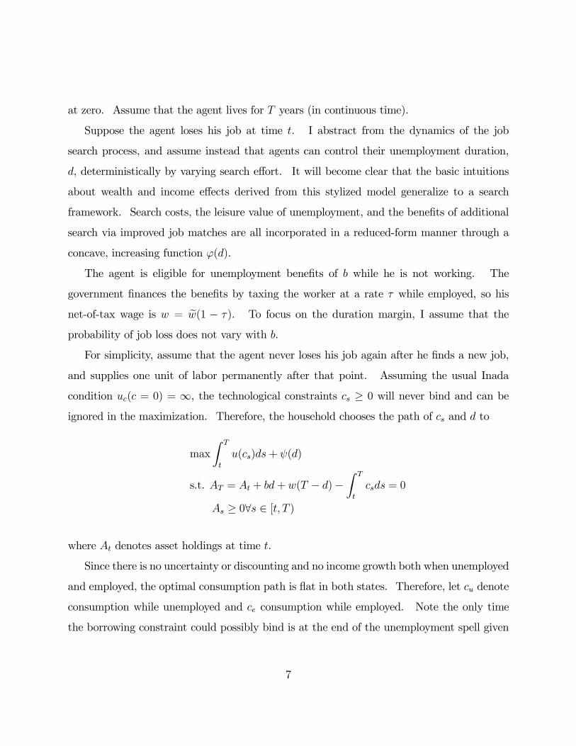
For simplicity, assume that the agent never loses his job again after he finds a new job,

and supplies one unit of labor permanently after that point. Assuming the usual Inada

condition uc(c = 0) = ∞, the technological constraints cs ≥ 0 will never bind and can beignored in the maximization. Therefore, the household chooses the path of cs and d to

max

Z T

t

u(cs)ds+ ψ(d)

s.t. AT = At + bd+ w(T − d)−Z T

t

csds = 0

As ≥ 0∀s ∈ [t, T )

where At denotes asset holdings at time t.

Since there is no uncertainty or discounting and no income growth both when unemployed

and employed, the optimal consumption path is flat in both states. Therefore, let cu denote

consumption while unemployed and ce consumption while employed. Note the only time

the borrowing constraint could possibly bind is at the end of the unemployment spell given

7

that the consumption path is flat in both states. The agent’s problem can be rewritten as

max du(cu) + (T − d)u(ce) + ψ(d)

s.t. [λ] AT = At + bd+ w(T − d)− dcu − (T − d)ce = 0 (1)

[µ] Ad = At + bd− dcu ≥ 0 (2)

Let λ denote the multiplier associated with the intertemporal budget constraint (1) and µ

the multiplier associated with the borrowing constraint (2) in period t. These multipliers

represent the marginal value of relaxing each of the constraints at the optimum in period t.

Let ∆u = u(ce)−u(cu) denote the change in the flow utility of consumption from the unem-ployed to the employed period. Taking the Kuhn-Tucker conditions for this maximization

problem, the following conditions must hold at the optimum:

u0(cu) = λ+ µ (3)

u0(ce) = λ (4)

ϕ0(d) = (λ+ µ)(w − b) + (λ+ µ)(cu − ce) +∆u (5)

The intuition for these optimality conditions can be seen with standard perturbation

arguments. First consider the case where (2) does not bind. If the borrowing constraint is

slack at the optimum, there cannot be any marginal value in loosening it further. Hence,

µ = 0 and u0(cu) = λ = u0(ce). Therefore the optimality condition for the duration choice

simplifies to ϕ0(d) = λ(w − b). Intuitively, the marginal benefit of remaining unemployed

one week longer should offset the marginal consumption utility loss of losing w−b in income.Now consider the case where the borrowing constraint (2) binds. In this case, the

provision of an extra dollar of wealth at time t relaxes both the borrowing constraint and

the intertemporal budget constraint, raising utility by λ + µ. Since it is strictly optimal

to consume that dollar immediately if the borrowing constraint is binding, the marginal

8

utility of consumption while unemployed must equal the sum of these two multipliers. But

additional wealth when employed does not relax the borrowing constraint, so u0(ce) = λ.

When the agent is constrained, the optimality condition for duration has additional terms

because the agent exhausts his assets before finding a new job and thus consumption is not

smooth over time: cu < ce = w.

Let g(·) denote the inverse of the ψ0(d) function and define Z = (λ + µ)(w − b) + (λ +µ)(cu − ce) +∆u. Then the agent’s unemployment duration can be written as

d = g(Z) (6)

This equation is very similar to the Frisch labor supply expression obtained from in-

tertemporal labor supply models (see MaCurdy 1981; Blundell and MaCurdy 1999). It

differs from the standard Frisch expression only because of the borrowing constraint. In

the unconstrained case, where Z = λ(w − b), the agent’s unemployment duration (or laborsupply) is fully determined by the marginal utility of wealth, λ, and the net wage, w − b.As originally shown by MaCurdy, this representation for the optimal labor supply decision

permits a transparent separation of wealth and substitution effects, because wealth effects

affect behavior only by changing λ. I now use this observation to compare the income effects

of UI benefits for constrained and unconstrained individuals.

2.1 Income Effect of UI Benefits on Durations

Unconstrained Case. Consider an individual for whom (2) does not bind at his optimal

allocation at the time of unemployment (µ = 0). Since wealth effects arise only through

changes in λ, the wealth (or income) effect of UI benefits on duration is given by

εINCd,b (µ = 0) =∂ log g

∂ logZ

∂ log λ

∂ logW

∂ logW

∂ log b

9

Define δ = − ∂ log g∂ logZ

. Let γW = − ∂ logλ∂ logW

denote the elasticity of the marginal utility

of wealth with respect to wealth, i.e. the coefficient of relative risk aversion of the value

function over wealth. With this notation,

εINCd,b (µ = 0) = δγWεW,b (7)

In the aggregate, UI is a balanced-budget transfer program, and thus induces no change

in lifetime wealth. Higher benefits are fully offset by higher taxes. Hence, in a benchmark

case with identical agents, εINCd,b = εW,b = 0. In an environment with heterogeneity, higher UI

benefits can generate increases in net wealth for some individuals. To bound the magnitude

of εINCd,b in this case, consider an increase in UI benefits for an individual without any change

in the UI tax. In this case, ∂W∂b= 1 and the εW,b parameter therefore equals the fraction of

lifetime wealth accounted for by UI benefits. To obtain a rough estimate of this fraction, I

use data on weeks of unemployment from the PSID for household heads followed from 1968

to 1998. Among individuals who report being unemployed at least once, the median number

of weeks unemployed between 1968 and 1998 is 32.5 and the mean is 50. Since the wage

replacement rate for UI is around 50% and males work for roughly 40 years, UI benefits

account for approximately 0.5×5040×52 = 1.2% of lifetime wealth. This is an upper bound because

we have ignored non-labor income and because not all weeks of unemployment are covered

by UI. Hence εW,b < 0.012, i.e. doubling UI benefits permanently raises lifetime wealth by

at most 1.2% for the mean job loser.

The small impact of UI benefits of lifetime wealth implies that UI has small income effects

on unemployment durations for unconstrained agents. This can be demonstrated formally

by bounding the other parameters in equation (7). To bound δ, let εd,b denote the total

elasticity of durations with respect to benefits, and recall that empirical studies of UI have

found εd,b ∈ (0.4, 0.8). Differentiating (6) w.r.t. b yields εd,b > − ∂ log g∂ logZ

bw−b , which implies

δ = − ∂ log g∂ logZ

< 1 given that bw' 1

2in practice. Given a plausible value for the coefficient of

10

relative risk aversion (e.g. γW < 5), it follows that εINCd,b < 0.06. Hence, a 10% increase in

UI benefits raises duration by at most 0.6% via the wealth effect. The lifetime wealth effect

thus accounts for a minor fraction of εd,b for the typical unconstrained UI claimant, even in

the extreme case where higher benefits are not offset at all by higher taxes.5

Constrained Case. Now consider an individual for whom (2) binds, perhaps because he

faced a series of bad wealth realizations or income shocks before period t, or because he has

a low discount factor β and chose not to build up a sufficiently large buffer stock to fully

smooth consumption during his current unemployment spell.6 Using the first-order Taylor

approximation ∆u = (λ+ µ)(ce − cu) and recalling that ce = w here, it follows that

εINCd,b (µ > 0) ' ∂ log g

∂ logZ

∂ log λ+ µ

∂ log cu

∂ log cu∂ log b

(8)

= δγcεcu,b (9)

where γc = −∂ log u0(cu)∂ log cu

denotes the coefficient of relative risk aversion over consumption

and εcu,b is the elasticity of consumption while unemployed with respect to benefits. This

elasticity could be an order of magnitude larger than the wealth effect for unconstrained in-

dividuals. To see this, first note that the γc > γW : since individuals can adjust labor supply

and other margins over their lifetime, the curvature of indirect utility over wealth must be

lower than the curvature of utility over consumption (see Bodie, Merton, and Samuleson 1992

and Chetty 2003). The ratio of the income elasticities for constrained and unconstrained

individuals therefore exceeds εcu,b/εW,b. Empirical studies of consumption-smoothing have

found that εcu,b > 0.2 among constrained groups. It follows that the income elasticity of UI

5Of course, individuals who are laid off very frequently (e.g. seasonal workers) might experience a signifi-cantly larger wealth effect from UI benefit changes. Although these responses do not arise from the constraintmechanism emphasized in this paper, they reinforce the general point that much of the UI-duration link couldbe due to non-distortionary income or wealth effects rather than substitution effects.

6The important question of why many job losers have virtually no assets is left to future research. Inthis study, I focus only on ex-post search behavior conditional on asset holdings, ignoring the reasons forinitial asset choices.

11

could be 10-20 times larger for constrained agents.

This simple analysis shows that UI benefits could have a non-trivial income effect on

durations when µ > 0. This effect occurs in addition to and independently of the usual

substitution effect. Intuitively, when the agent relies on unemployment benefits to maintain

consumption, raising the benefit level has a large effect on consumption while unemployed.

This reduces the pressure to find a job quickly in order to generate consumption, creating

the potential for an income effect. In contrast, when agents are unconstrained, the income

effect channel is virtually shut down because UI benefits are a trivial fraction of lifetime

wealth and have little effect on consumption while unemployed.

Deadweight cost of UI benefits. As with any tax or benefit program, the deadweight

cost of UI is determined strictly by the size of the substitution elasticity and not the income

elasticity. Intuitively, an efficiency cost is generated only when individuals’ respond to a

wedge between private and social marginal costs, i.e. substitution in response to changes in

relative prices. More precisely, observe that the efficiency cost of UI can be defined as the

loss in welfare from having a benefit proportional to duration instead of a lump-sum grant

at the time of job loss of an equivalent amount (Bi = b× di). If the proportional UI benefitaffects search behavior only through an income effect, replacing it with a lump-sum benefit

would leave behavior and welfare unchanged. But if UI affects search behavior through a

substitution effect, a lump-sum benefit would make agents voluntarily reduce unemployment

durations while keeping income in the unemployed state constant, thereby raising welfare.

Hence, the efficiency cost arises purely from the substitution effect.7

The remainder of the paper focuses on estimating the income and substitution elasticities

to shed light on the efficiency cost of UI.

7In a second-best world with liquidity constraints (a market failure), UI benefits can raise welfare byproviding liquidity. This welfare change is independent of the potential efficiency loss generated by UI.

12

3 Empirical Analysis I: The Role of Constraints

3.1 Estimation Strategy

The model suggests a natural first step to evaluating whether constraints and income effects

play a role in the UI-duration link: Estimate the effect of UI benefits on durations for

constrained individuals (µ > 0) and unconstrained individuals (µ = 0) separately. If the

UI-duration link is driven primarily by the µ = 0 group, it would be implausible that

income effects are important; but if the link comes from the µ > 0 group, income effects

might matter. This heterogeneity analysis essentially replicates the standard difference-in-

difference methodology using UI law variation (as in Meyer 1990) on various subsets of the

data.

I divide individuals into unconstrained and constrained groups and estimate equations of

the following form:

log dit = β0 + β1 log b+ β2Xi,t + θi,t (10)

where Xi,t denotes the observable component of the taste shift variable for household i and

θi,t = Θi,t−β2Xi,t denotes the component of that variable that cannot be observed in the data.The key identifying assumption for the empirical analysis is the same as that underlying the

conventional difference-in-difference strategy of Moffit, Meyer and others. The UI benefit

rate must be orthogonal to unobserved variation in tastes:

Eb× θi,t = 0 (11)

Some evidence supporting this assumption is described in the next section.

For simplicity, I ignore the small lifetime wealth effect of a change in UI benefits for

unconstrained individuals by assuming εINCd,b (µ = 0) = 0 below. This assumption leads us to

slightly overstate the true magnitude of substitution effects and understate the magnitude

of income effects. With this simplification, when (10) is estimated for the unconstrained

13

(µ = 0) group, the coefficient

βµ=01 = εµ=0d,b = εs,µ=0d,b

gives the pure substitution effect of UI benefits on unemployment durations for unconstrained

individuals.

When (10) is estimated for a group of constrained individuals (µ > 0), we obtain

βµ>01 = εµ>0d,b = εs+I,µ>0d,b

which is an estimate of the composite effect of UI on durations for this group, including both

substitution and income effects. The composition of this elasticity in terms of the income

and substitution components cannot be identified with the empirical strategy implemented

in this section. The second empirical strategy (section 4) decomposes this elasticity into an

income and substitution effect using variation in lump-sum severance payments.

One might wonder why I focus on UI benefits to test whether cash-on-hand affects un-

employment durations, rather than using variation in wealth holdings more generally. The

main reason is that the variation in UI benefits is credibly exogenous, insofar as it comes

from differences across states and time in laws. In contrast, wealth holdings at the time

of unemployment are endogenous and correlated with other factors that could influence du-

rations such as skills. Indeed, Gruber (2001) finds that agents with low levels of wealth

also tend to have short job tenures and limited labor force experience, inducing a negative

correlation between wealth and duration.8

Defining the constrained group. The main difficulty in implementing (10) is that µ is

a latent variable, making it impossible to classify households into groups directly based on

whether they face a binding borrowing constraint. Therefore, following Zeldes (1989), I use

a set of proxies that are predictors of whether a household is constrained. The primary

8This endogeneity problem could explain why Lentz (2003) and others generally find little associationbetween wealth holdings and unemployment durations in the cross-section.

14

proxy is liquid wealth net of unsecured debt, which I term “net wealth.” Households that

have higher levels of net wealth (Ai,t) at the time of job loss are less likely to be constrained,

allowing them to smooth consumption provided that the spell is not too long. In contrast,

households with low assets, especially Ai,t < 0, are likely to be completely reliant on UI

income for consumption while unemployed, making µ > 0 for many of them. As a robustness

check, I also proxy for constraints using net liquid wealth divided by pre-unemployment wage.

This measure captures how much of the lost income each household can replace using its

assets (Gruber, 2001). Results with this alternative definition (not reported) are very similar

to the simple asset cuts.

The second proxy is whether the individual has a spouse who is also working prior to

job loss. Households that rely on a single income are more likely to be constrained when

that individual loses his job; those with an alternate source of income may have additional

sources of liquidity, including better access to credit because at least one person has a stable

job. The third proxy for µ is the household’s mortgage payments. Gruber (1998) finds

that fewer than 5% of the unemployed sell their homes during a spell. Consequently, if an

individual must make large mortgage payments, he effectively has less liquid wealth, and is

more likely to be constrained than a renter who can move more easily or a homeowner who

has to make no mortgage payments.

The validity of each of these variables as proxies for being constrained by UI income is

substantiated by the results of Browning and Crossley (2001), who find a positive association

between UI benefits and consumption precisely when households have low-assets or only

one earner.9 Nonetheless, these markers are imperfect predictors of who is constrained.

Some households with µ = 0 are presumably misallocated to the µ > 0 group and vice-

versa. Such classification error will pull the estimated elasticities for the two groups closer

together, thereby causing us to underestimate the importance of liquidity constraints in the

9Unfortunately, the SIPP lacks consumption data, so their findings cannot be directly corroborated forthis sample.

15

UI-duration link.

Note that these proxies for constraints are all endogenous to the agent’s underlying

preferences and behavior: agents can choose, to some degree, their assets, mortgage status,

and spousal work status. Since these proxies are not exogenously assigned, differences in

behavior across groups (e.g. low asset vs. high asset) may be due to the unobservables that

led some households to be constrained and others to be unconstrained. Hence, the group-

specific elasticity estimates below are informative about the potential for income effects but

have less to say about the causality of constraints — that is, the estimates do not tell us

how the behavior of the unemployed would change if liquidity constraints were exogenously

tightened.

A concern in implementing (10) is that households may move across groups as an un-

employment spell elapses. Although the simple model above assumes that households can

anticipate their unemployment durations perfectly at the time of job loss, search is a dynamic

process in practice and households update their expectations over time while depleting their

buffer stocks. In this setting, the probability that a household faces a constraint will rise as

the spell elapses. Since the SIPP contains full asset data only at one point, the only feasible

way to account for this effect is by estimating models that allow UI benefits to have a time-

varying effect on unemployment exit rates. This concern, and more importantly the fact

that many unemployment spells are censored in the data, motivates estimation of a hazard

model with time-varying covariates rather than estimation of (10) using OLS. Letting hi,s

denote the unemployment exit hazard rate for household i in week s of an unemployment

spell and Xi,s denote a set of controls, the primary estimating equation for the constraint

tests is thus

hi,s = f(bi, s× bi, Xi,s) (12)

By estimating (12) for each of the groups defined by the proxies of µ described above,

we can recover the income and substitution elasticities of interest. While this reduced-form

16

approach does not permit complete recovery of the structural parameters needed to make

welfare calculations and analyze optimal UI policy numerically, it provides a transparent

means of illustrating the main features of the data.

3.2 Data

The data used to implement the constraint tests are from the 1985-1987, 1990-1993, and

1996 panels of the Survey of Income and Program Participation (SIPP). The SIPP collects

information from a sample of approximately 30,000 households every four months for a period

of two to three years. The interviews I use span the period from the beginning of 1985 to

the middle of 2000. At each interview, households are asked questions about their activities

during the past four months, including weekly labor force status. Unemployed individuals

are asked whether they received unemployment benefits in each month. Other data about

the demographic and economic characteristics of each household member are also collected.

I make five exclusions on the original sample of job leavers to arrive at my core sample.

First, following previous studies of UI, I restrict attention to prime-age males (over 18 and

under 65). Second, I include only the set of individuals who report searching for a job at

some point after losing their job, in order to eliminate individuals who have dropped out

of the labor force. Third, I exclude individuals who report that they were on temporary

layoff at any point during their spells, since they might not have been actively searching for

a job.10 Fourth, I exclude individuals who have less than three months work history within

the survey because there is insufficient information to estimate pre-unemployment wages for

this group. Finally, I focus primarily on individuals who take up UI within one month

after losing their job because it is unclear how UI should affect hazards for individuals who

10Katz and Meyer (1990) show that whether an individual considers himself to be on temporary layoff isendogenous to the duration of the spell; recall may be expected early in a spell but not after some time haselapsed since a layoff. Excluding temporary layoffs can therefore potentially bias the estimates. To checkthat this is not the case, I include temporary layoffs in some specifications of the model.

17

delay takeup. The potential sample selection bias related to UI takeup that arises from this

exclusion is addressed below.

These exclusions leave 4,560 individuals in the core sample. Note that asset data is

generally collected only once in each panel, so pre-unemployment asset data is available

for approximately half of these observations. The first column of Table 1 gives summary

statistics for the core sample, which looks reasonably representative of the general population.

The median UI recipient is a high school graduate and has pre-UI gross annual earnings

of $20,726 in 1990 dollars. The most germane statistic for the present analysis is pre-

unemployment wealth: median liquid wealth net of unsecured debt is only $128.

The raw data on UI laws were obtained from the Employment and Training Administra-

tion (various years), and supplemented with information directly from individual states.11

The computation of weekly benefit amounts deserves special mention. Measurement er-

ror and inadequate information about pre-unemployment wages for many claimants make it

difficult to simulate the potential UI benefit level for each agent precisely. I therefore use

three approaches to proxy for each claimant’s (unobserved) actual UI benefits, all of which

yield similar results. First, I use published average benefits for each state/year pair in lieu

of each individual’s actual UI benefit amount. Second, I proxy for the actual benefit using

maximum weekly benefit amounts, which are the primary source of variation in benefit levels

across states. Most states replace 50% of a claimant’s wages up to a maximum benefit level.

The third method involves simulating each individual’s weekly UI benefit using a two-stage

procedure. In the first stage, I predict the claimant’s pre-unemployment annual income

using information on education, age, tenure, occupation, industry, and other demographics.

The prediction equation for pre-UI annual earnings is estimated on the full sample of individ-

uals who report a job loss at some point during the sample period.12 In the second stage, I

11I am grateful to Julie Cullen and Jon Gruber for sharing their simulation programs, and to SuzanneSimonetta and Loryn Lancaster in the Department of Labor for providing detailed information about stateUI laws from 1984-2000.12Since many individuals in the sample do not have a full year’s earning’s history before a job separation,

18

use the predicted wage as a proxy for the true wage, and assign the claimant unemployment

benefits using the simulation program.

3.3 Results

3.3.1 Graphical Evidence and Non-Parametric Tests

I begin by providing graphical evidence on the benefit elasticity of unemployment durations

in constrained and unconstrained groups. I then show the robustness of these results to

controls, sample selection, and other potential specification concerns. First consider the

asset proxy for constraints. I divide households into four quartiles based on their net liquid

wealth (liquid wealth minus unsecured debt). Table 1a shows summary statistics for each

of the four quartiles. Although the households in the lower net liquid wealth quartiles are

slightly poorer and less educated, the differences between the four groups are not extremely

large. Notably, quartiles 1 and 3 are very similar in terms of income, education, and other

demographics. Hence, UI benefits are similar both in levels and as a fraction of permanent

income for all the groups.

Figures 1a-d show the effect of UI benefits on unemployment exit rates for households

in the each of the four quartiles of the net wealth distribution. To construct Figure 1a, I

first divide the observations into two categories: Those that are in (state, year) pairs that

have average weekly benefit amounts above the sample median and those below the median.

Kaplan-Meier survival curves are then plotted for these two groups using the households in

the lowest quartile of the net wealth distribution. This procedure is repeated for the other

three quartiles of the net wealth distribution to construct Figures 1b-d. Since asset levels

may be endogenous to the length of durations, households for whom asset data are available

only after job loss are excluded when constructing these figures. Including these households

I define the annual income of these individuals by assuming that they earned the average wage they reportbefore they began participating in the SIPP. For example, individuals with one quarter of wage history areassumed to have an annual income of four times that quarter’s income.

19

turns out to have little effect on the qualitative results (as we will see below in the regression

analysis).

These and all subsequent survival curves plotted using the SIPP data are adjusted for the

“seam effect” common in panel datasets. Individuals are interviewed at 4 month intervals

in the SIPP and tend to repeat answers about weekly job status in the past four months

(the “reference period”). As a result, they under-report transitions in labor force status

within reference periods and overreport transitions on the “seam” between reference periods.

Consequently, a disproportionately large number of spells appear to last for exactly 4 or 8

months in the data. These artificial spikes in the hazard rate are smoothed out by first

fitting a Cox model with a time-varying indicator variable for being on a seam between

interviews, and then recovering the (nonparametric) baseline hazards to construct a seam-

adjusted Kaplan-Meier curve. The resulting survival curves give the probability of remaining

unemployed after t weeks for an individual who never crosses an interview seam. Note that

the results are qualitatively similar if the raw data is used without any adjustment for the

seam effect.

Figure 1a shows that higher UI benefits are associated with much lower unemployment

exit rates for individuals in the lowest wealth quartile, who are most likely to be in the

constrained group (µ > 0). For example, after 15 weeks, 55% of individuals in low-

benefit state/years are still unemployed, compared with 68% of individuals in high-benefit

state/years. A nonparametric Wilcoxon test rejects the null hypothesis that the two survival

curves are identical with p < 0.01. Figure 1b constructs the same survival curves for the

second wealth quartile. UI benefits appear to have a smaller, but still powerful effect on

durations in this group. At 15 weeks, 63% of individuals in the low-benefit group are still

unemployed, vs. 70% in the high benefit group. The Wilcoxon test again rejects equality

of the survival curves in this group, with p = 0.04. Figure 1c shows that effect of UI on

durations virtually disappears in the third quartile of the wealth distribution. At 15 weeks,

57% of those in low-benefit states have found a job, vs. 59% in high-benefit states. Not

20

surprisingly, the Wilcoxon test does not reject equality of these survival curves (p = 0.74).

Finally, Figure 1d shows that UI appears to have no effect on durations for the richest group

of households, who are least likely to be constrained (µ = 0). In both the high-benefit

and low-benefit groups, 64% of the job losers remain unemployed after 15 weeks, and the

Wilcoxon test does not reject equality (p = 0.43). The fact that UI has little effect on

durations in the unconstrained groups suggests that it induces little or no substitution effect

among households with sufficient resources to smooth consumption while unemployed.

I now replicate these graphs and nonparametric tests for the other two proxies of con-

straints. Table 1b shows summary statistics for the constrained and unconstrained groups

based on spousal work and mortgage status. As with the asset cuts, there are differences

across the constrained and unconstrained groups in income and education, but these are not

extremely large. Figures 2a-b compare the effect of UI on unemployment exit rates for single

and dual-earner households. Figure 2a shows that UI benefits significantly reduce exit rates

for households who are more likely to be constrained at the time of job loss because they

were relying on a single source of income. The Wilcoxon test rejects equality of the survival

curves with p < 0.01. In contrast, UI benefits appear to have no effect on exit hazards for

households with two earners (Figure 2b).

The results for the mortgage cut are similar. Figure 3a shows that UI benefits have

a sharp effect on durations among households that have a mortgage to pay off at the time

of job loss, and equality of the two survival curves is again rejected with p < 0.01. But

among households without a mortgage pre-unemployment, the difference between the sur-

vival curves in the high-benefit and low-benefit groups is much smaller and statistically

indistinguishable (Figure 3b). Note that the constrained types in this cut, who are home-

owners with mortgages, have higher income, education, and wealth than the unconstrained

types, who are primarily renters (see Table 1b). This is in contrast with the asset and

spousal work proxies, where the constrained group included more households with lower

income, education, and wealth. This makes it somewhat less likely that the differences in

21

the benefit elasticity of duration across constrained and unconstrained groups is spuriously

driven by other differences across the groups such as income or education.

As noted above, an important assumption in this analysis is that the variation in UI

benefits is orthogonal to other unobservable determinants of durations, i.e. that (11) holds.

To test this identification assumption, Figure 4 shows the effect of UI benefits on durations

for a “control group” of below-median net wealth individuals who do not receive UI benefits,

either because of ineligibility or because they chose not to take up.13 The durations of these

individuals are insensitive to the level of benefits, supporting the claim that UI benefits play

a causal role in increasing durations among constrained households who receive benefits.

3.3.2 Semi-Parametric Estimates

I evaluate the robustness of the graphical results by estimating (12) using a Cox specification

for the hazard function. The Cox model assumes a proportional-hazards form for the hazard

rate s weeks after unemployment:

log hi,s = αs + β1 log bi + β2s× log bi + β3Xi,s (13)

whereXi,s denotes a set of covariates and {αs} are the set of baseline hazards. The coefficientof interest is β1, which captures the effect of raising the log of the UI benefit assigned to

individual i. To control for the fact that the relationship between UI benefits and the hazard

rate may vary over time, the model also includes an interaction of log(bi) with s, the weeks

elapsed since job loss. Note that this specification does not impose any functional form on

the baseline unemployment exit rates in each week, so the coefficients on the key covariates

are identified purely from variation in UI laws, as in the graphical analysis. Tables 2 and 3

13Results are similar for the set of job losers who are ineligible for UI, who arguably are a better “control”because takeup of UI is endogenous. However, the UI-ineligible group consists of part-time workers whohave very low levels of earned income before unemployment and may therefore not be similar to the averageUI claimant.

22

presents estimates of (13) and variants of this basic specification which are described below.

I first estimate (13) on the full sample to identify the unconditional effect of UI on the

hazard rate. In this specification, as in most others, I use the average UI benefit level in the

individual’s (state,year) pair to proxy for bi in light of the measurement-error issues discussed

in the data section. This specification includes a full set of controls: Industry, occupation,

and year dummies; a 10 piece log-linear spline for the claimant’s pre-unemployment wage;

linear controls for total (illiquid+liquid) wealth, age, education; and dummies for marital

status, pre-unemployment spousal work status, and being on the seam between interviews

to adjust for the seam effect. Standard errors in this and all subsequent specifications are

clustered by state.

The coefficients reported Table 1 and all subsequent tables are estimates of β1, which can

be interpreted as elasticity of the hazard rate with respect to UI benefits. The estimate in

column 1 of Table 2a indicates that a 10% increase in the UI benefit rate reduces the hazard

rate by approximately 4% in the pooled sample. Reassuringly, this unconditional estimate

is in the range found by Moffitt (1985), Meyer (1990), and Katz and Meyer (1990).

Heterogeneity by Net Liquid Wealth Quartiles. I now examine the heterogeneity of the

UI effect by estimating separate coefficients for constrained and unconstrained groups as in

the graphical analysis. Table 2 considers the asset proxy for constraints by dividing the

data into four quartiles of the net wealth distribution as in the graphical analysis. Let

Qi,j denote an indicator variable that is 1 if agent i belongs to quartile j of the wealth

distribution. Let αs,j denote the baseline exit hazard for individuals in quartile j in week

s of the unemployment spell. To avoid parametric restrictions, the baseline hazards are

allowed to vary arbitrarily across the constrained and unconstrained groups. Columns 2-5

of Table 2 report estimates of the following stratified Cox regression:

log hi,s = αs,j + βj1Qi,j log bi + βj2Qi,j(s× log bi) + β3Xi,s (14)

23

Specification (2) of Table 2a estimates this equation with no controls (no X). The key

coefficients of interest are {βj1}j=1,2,3,4, which tell us the effect of raising UI benefits on thehazard rate for each quartile of the net wealth distribution. The estimates indicate that βj1

is rising in j, i.e. the effect of UI benefits monotonically declines as one moves up in the

net liquid wealth distribution. Among households in the lowest quartile of net wealth, a

10% increase in UI benefits reduces the hazard rate by 7.9%, an estimate that is statistically

significant at the 5% level. In contrast, there is a small, statistically insignificant association

between the level of UI benefits and the hazard among households in the third and fourth

quartiles of net wealth. The null hypothesis that UI benefits have the same effect on hazard

rates in the first and fourth quartiles is rejected with p < 0.05, as is the null hypothesis that

the mean UI effect for below-median wealth households is the same as that for above-median

wealth households. These findings support the conclusion drawn from the graphical analysis

that UI benefits have much stronger effects on durations for households constrained by low

net liquid wealth.

Specification (3) replicates the preceding specification with the full set of controls used

in column (1). The key coefficients of interest are virtually unchanged when this rich set

of covariates is introduced. The fact that controlling for observed heterogeneity does not

affect the results suggests that the estimates are unlikely to be very sensitive to unobservable

heterogeneity as well.

The preceding specifications maximize sample size by using data on post-unemployment

assets for households where pre-unemployment asset data are unavailable. Since post-

unemployment assets may be endogenous to the agent’s spell length, this form of sample

selection could yield biased results. Specification (4) addresses this concern by estimating

(3) on the subsample of households with pre-unemployment asset data. Since the sample

size is reduced by more than 50%, the standard errors in this specification are larger. How-

ever, the pattern of the coefficients remains very similar to that in specification (3). The

hypothesis that the effect of UI on exit rates of below-median wealth and above-median

24

wealth households is the same can be rejected with p = 0.05.

Specification (5) introduces state fixed effects in addition to the full set of controls. In

this model, the variation in the UI benefit level comes purely from within-state law changes.

Results remain similar, with monotonically increasing βj1 coefficients as wealth rises.

Table 2b reports a series of additional robustness checks for the asset heterogeneity tests.

All of these specifications include the full control set. Specification (1) restricts the sample

to low-wage households, dropping individuals who report pre-unemployment annual wages

above $24,720, the 75th percentile of the wage distribution. The goal of this specification

is to address the concern that substitution effects of UI benefits could differ for individuals

with different wage rates. For example, UI benefits may be a small fraction of income for

high-income households and may therefore have little effect on their search behavior. Since

high income households tend to be somewhat over-represented in the high asset quartiles,

this alternative hypothesis could be responsible for the results. The estimates in column 1

reject this alternative explanation, since UI benefits continue to have much stronger effects

among low-asset households when high income households are excluded.

Columns (2) and (3) examine robustness to changes in the definition of bi. Column

(2) uses the maximum UI benefit level in individual i’s state/year and column (3) uses the

simulated benefit for each individual i using the two-stage procedure described above. Both

specifications give similar results to the baseline case. Column (4) shows that including

individuals who report being on temporary layoff does not affect the results.

Finally, column (5) replicates the baseline specification but defines the quartiles of wealth

in terms of home equity rather than net liquid wealth and restricts the sample to homeown-

ers. Home equity is much less accessible than liquid wealth during an unemployment spell,

since borrowing even against secured assets is difficult when one is unemployed. Home

equity should therefore be a poorer predictor of liquidity constraints than liquid wealth. If

constraints play a role in the UI-duration link, the differences in the effect of UI benefits

across quartiles of home equity should be weak. In contrast, if the preceding results are due

25

to spurious correlations between the benefit elasticity of durations and income or wealth, the

home equity and liquid wealth cuts should produce the same results. The evidence suggests

a role for borrowing constraints, as there is no strong pattern in the coefficients on the UI

benefit variable across the quartiles in column 5.

As a robustness check, I predict assets based on age, income, education, and marital

status. I then define net liquid wealth quartiles on the basis of predicted wealth and replicate

the preceding analysis. This analysis is particularly useful in conjunction with the severance

pay evidence in section 4, where households are classified into groups based on the same asset

prediction equation. Results from this procedure (not reported) are generally quite similar

to those above. Individual predictors of assets also support the basic results. For example,

the effect of UI benefits on durations is much stronger among individuals younger than the

median age (31 years) — who have much fewer assets on average — than among those above

the median age.

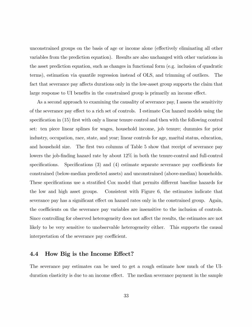
Spousal Work Status. Table 3a reports estimates of specifications analogous to (14) for

the spousal work proxy. Instead of quartiles of liquid wealth, the UI benefit coefficient

is interacted with a dummy for whether the agent lived in a single-earner or dual-earner

household prior to job loss. The baseline hazards are also stratified by this dummy. The

first specification includes all observations in the core sample without any controls. In this

group, there is a moderate but statistically insignificant difference in the UI benefit coefficient

for the single-earner and dual-earner groups.

To explore this result in greater detail, observe that households with very low net wealth

(who typically have substantial debt) are likely to be constrained irrespective of whether

they have two earners or not, and households with very high net wealth are likely to be

unconstrained regardless of spousal work status. Specification (2) therefore focuses on

households in the middle two quartiles of the net wealth distribution, who are most likely to

be on the margin of being liquidity constrained. In this subgroup of households, the effect

of spousal work status emerges much more clearly. A 10% increase in the UI benefit reduces

26

the mean unemployment exit hazard by 5.5% for single-earners but has a small, statistically

insignificant effect for dual earners. The null hypothesis that the effect is identical in the

two groups is rejected with p = 0.06. The third column shows that this result is robust

to including the full set of controls described above. The fourth column adds state fixed

effects, and shows that the general pattern is preserved although standard errors rise in this

specification. Column 5 restricts attention to the households in the lowest quartile of net

wealth. Consistent with the hypothesis that these households are constrained regardless of

spousal work status, UI benefits have a strong effect on durations in both single-earner and

dual-earner families in this category.

Mortgage Status. Table 3b shows results for the mortgage proxy using the observations

for which pre-unemployment mortgage data is available. The first specification supports

the graphical evidence in Figure 3, indicating that UI benefits have a much larger effect

on durations among households that have mortgages. Equality of coefficients on the UI

benefit variable among mortgage-holders and non-holders is rejected with p < 0.01. The

second and third specifications confirm that this result is robust to the full set of controls

and state fixed effects. The fourth specification includes only households with net liquid

wealth below the sample median. The estimates indicate that low-wealth households who

have to pay a mortgage — who are perhaps especially constrained — are extremely sensitive

to unemployment benefits in their search behavior.

Sample Selection Concerns. One might worry that endogeneity of takeup with respect

to the level of benefits biases the estimate of the UI benefit elasticity. In my sample, a 10%

increase in the benefit rate is associated with a 1% increase in the probability of UI takeup

in the first month of unemployment.14 If the marginal individuals who decide to take up

UI when benefits rise tend to have shorter unemployment spells on average, estimates of the

14The probability of taking up UI at any point during the spell rises by 2% for a 10% increase in UIbenefits. This is exactly equal to the estimate reported by Anderson and Meyer (1997), who use a muchlarger dataset on benefit takeup.

27

UI benefit elasticity will be biased toward zero.

This issue is unlikely to affect the results above for two reasons. First, the takeup elasticity

is similar across all the constrained and unconstrained subgroups. Hence, there is no reason

that it should artificially bias down the estimate only in the unconstrained group. Second,

even if there were differential biases across groups, the effects on the estimated UI benefit

elasticity would be quite small. The magnitude of the bias can be gauged by assuming that

the individuals who are added to the sample through this selection effect are drawn randomly

from the group who do not takeup UI. The empirical hazards for the non-UI group are on

average 1.1 times as large as those of the UI recipients. In practice, the marginal individual

who takes up UI is likely to anticipate a longer UI spell than the average agent who does

not take up UI, so the 1.1 ratio provides an upper bound for the size of the selection bias.

Starting from an initial takeup rate of 50%, a 10% increase in benefits will cause the average

hazard rate to rise through this selection effect by approximately 1%50%∗ (1.1 − 1) = 0.2%.

But the difference in the hazard rates across constrained and unconstrained groups induced

by a 10% benefit increase was an order of magnitude larger (approximately 5%), suggesting

that this selection effect is not critical.

In summary, there is strong evidence that UI benefits (1) induce small substitution ef-

fects among households likely to be unconstrained; and (2) induce large responses among

households that are likely to be constrained.

4 Empirical Analysis II: Severance Pay and Durations

While the preceding evidence shows that constraints play a role in the UI-duration link, it

does not directly establish that the income elasticity of unemployment durations is large

among constrained households. This section complements the preceding analysis by testing

whether the large duration response in constrained households does indeed arise from an

income effect.

28

4.1 Estimation Strategy

Many firms in the United States have severance packages that compensate employees who

are laid off. According to a recent survey of Fortune 1000 firms (Lee Hecht Harrisson 2001),

the most common policy for regular (non-executive) full-time workers is a severance payment

of one week of pay for each year of service at the firm. However, some companies have flatter

or steeper severance pay profiles with respect to job tenure. Many companies have minimum

job tenure thresholds to be eligible for severance pay (e.g. 3 years or 5 years). For regular

salaried employees, there is very little variation in severance packages within a given firm and

tenure bracket (presumably because individuals are reluctant to negotiate with firms about

severance pay). Hence, conditional on tenure, the primary source of variation in severance

pay comes from cross-firm differences in policies.15

The key characteristic of severance payments for the present analysis is that they are

lump-sum, i.e. they are not proportional to the length of unemployment spells. Receipt of

standard tenure-based severance pay does not delay eligibility for UI benefits.16 Severance

payments therefore have pure income effects and do not distort the relative price of consump-

tion and leisure for unemployed agents. I estimate the income elasticity of unemployment

durations using models similar to those above, changing the key independent variable from

the UI benefit to sevi, a dummy for receipt of severance pay:

hi,s = αs exp(θ1sevi + θ2Xi,s) (15)

The coefficient θ reveals the causal effect of severance pay on unemployment exit hazards if

receipt of severance pay is orthogonal to other determinants of durations. After estimating

the baseline model, tests of the orthogonality condition are discussed.

15There is also variation in the amounts of severance payments, but the data on amounts is too sparse tobe useful.16This can be confirmed in the data: There is no correlation between receipt of severance pay and the

length of time from job loss to first UI payment.

29

4.2 Data

The data for this portion of the study come from two surveys conducted by Mathematica on

behalf of the Department of Labor, matched with administrative data from state UI records.

The first dataset is the “Study of Unemployment Insurance Exhaustees,” which contains

data on the unemployment durations of 3,907 individuals who claimed UI benefits in 1998.

This dataset is a sample of unemployment durations in 25 states of the United States, with

oversampling of individuals who exhausted UI benefits. In addition to administrative data

on prior wages and weeks of UI paid, there are a large set of survey variables that give

information on demographic characteristics, household income, job characteristics (tenure,

occupation, industry), and most importantly for this study, receipt of severance pay.

The second dataset is the “Pennsylvania Reemployment Bonus Demonstration.” This

data was collected as part of an experiment to evaluate the effect of job reemployment

bonuses on search behavior. It contains information on 5,678 durations for a representative

sample of job losers in Pennsylvania in 1991. The information in the dataset is similar to

that in the exhaustees study.

For comparability to the preceding results, I make the same exclusions after pooling the

two datasets to arrive at the final sample used in the analysis.17 First, I include only prime-

age males. Second, I exclude temporary layoffs by discarding all individuals who expected

a recall at the time of layoff, but check to make sure that including these observations do

not change the results. These exclusions leave 2,730 individuals in the sample, of whom 521

report receiving a severance payment at job loss. Throughout the analysis, the data are

reweighted using the sampling weights to obtain estimates for a representative sample of job

losers.

Two measures of “unemployment duration” are available in this data. The first is the

number of weeks for which UI benefits were paid in the base year. This definition has

17I show only the results for the pooled data below, but similar results are obtained within each of thetwo datasets.

30

the advantage of accuracy since it comes from administrative records. It also has two

disadvantages: it is censored at the time of benefit exhaustion, and it captures total weeks

unemployed in a given year rather than the length of a particular spell (which could be

different for individuals with multiple short spells). The second measure is the survey

measure, constructed from individual’s recollection (typically one-two years after the job

loss event) of when they lost their initial job and when they found a new one. I focus on

the administrative measure here given its accuracy. However, results are quite similar (with

larger standard errors) for the survey measure.

Table 4 shows summary statistics for severance pay recipients and non-recipients. The

sample generally looks quite similar on observables to the SIPP sample used above. Given

the minimum tenure eligibility requirement, it is not surprising that severance pay recipients

have much higher median job tenures than non-recipients. Correspondingly, severance pay

recipients are older and higher in observable characteristics than non-recipients.

4.3 Results

I begin again with some graphical evidence. Figure 5 shows Kaplan-Meier survival curves

for two groups of individuals: those who received severance pay and those who did not.

Since pre-unemployment job tenure is an important determinant of severance pay and is also

highly positively correlated with durations, I control for it throughout. These survival curves

have been adjusted for tenure by fitting a cox model with tenure as the only regressor and

recovering the baseline hazards for each group. Severance pay recipients have significantly

lower unemployment exit rates. As a result, 66% of individuals who received severance pay

claimed more than 10 weeks of UI benefits, compared with 59% among those who received

no severance payment. Equality of the two survival curves is rejected by a nonparametric

test with p < 0.01.

An obvious concern with this result is that it may reflect correlation (via omitted vari-

31

ables) rather than causality because severance pay recipients differ from non-recipients in

many respects. As noted above, conditional on tenure, severance pay is determined primar-

ily by firms and is therefore unlikely to be correlated with individual-specific characteristics.

Hence, any omitted-variables explanation of the results must arise primarily from differences

between firms that pay severance and those that do not. A plausible alternative explanation

of the result is that firms that offer severance packages require very specific skills, making it

difficult for job losers to find new jobs, leading to long durations.

I use two approaches to examine the causality of severance pay. First, I investigate

whether the effect of severance pay differs across constrained and unconstrained groups.

The model in section 2 indicates that severance pay — which is a minor part of lifetime

wealth — should causally affect durations only among liquidity-constrained households. In

contrast, there is no reason to expect a differential effect of severance pay across constrained

and unconstrained households under the alternative explanation described above. Hence,

studying the heterogeneity of the severance pay effect provides a means of distinguishing

between the causal and most natural omitted-variable hypotheses.

Implementing this test requires division of households into constrained and unconstrained

groups. Unfortunately, the Mathematica surveys do not contain data on assets and the other

proxies for liquidity constraints used in the SIPP data. To overcome this problem, I predict

assets for each household with an equation estimated using OLS on the SIPP sample. The

prediction equation is a linear function of age, wage, education, and marital status. I then

divide households into two groups: Those with predicted assets above the median and those

with predicted assets below the median. Figures 6a-b replicate Figure 5 for these two groups.

They plot survival curves by severance pay after controlling for tenure. Figure 6a shows

that receipt of severance pay is associated with a large and statistically significant increase in

survival probabilities for constrained (low asset) households. Figure 6b shows that severance

pay has little effect on search behavior for households that are likely to be wealthier. As

in the UI benefit analysis, results are similar if households are split into constrained and

32

unconstrained groups on the basis of age or income alone (effectively eliminating all other

variables from the prediction equation). Results are also unchanged with other variations in

the asset prediction equation, such as changes in functional form (e.g. inclusion of quadratic

terms), estimation via quantile regression instead of OLS, and trimming of outliers. The

fact that severance pay affects durations only in the low-asset group supports the claim that

large response to UI benefits in the constrained group is primarily an income effect.

As a second approach to examining the causality of severance pay, I assess the sensitivity

of the severance pay effect to a rich set of controls. I estimate Cox hazard models using the

specification in (15) first with only a linear tenure control and then with the following control

set: ten piece linear splines for wages, household income, job tenure; dummies for prior

industry, occupation, race, state, and year; linear controls for age, marital status, education,

and household size. The first two columns of Table 5 show that receipt of severance pay

lowers the job-finding hazard rate by about 12% in both the tenure-control and full-control

specifications. Specifications (3) and (4) estimate separate severance pay coefficients for

constrained (below-median predicted assets) and unconstrained (above-median) households.

These specifications use a stratified Cox model that permits different baseline hazards for

the low and high asset groups. Consistent with Figure 6, the estimates indicate that

severance pay has a significant effect on hazard rates only in the constrained group. Again,

the coefficients on the severance pay variables are insensitive to the inclusion of controls.

Since controlling for observed heterogeneity does not affect the results, the estimates are not

likely to be very sensitive to unobservable heterogeneity either. This supports the causal

interpretation of the severance pay coefficient.

4.4 How Big is the Income Effect?

The severance pay estimates can be used to get a rough estimate how much of the UI-

duration elasticity is due to an income effect. The median severance payment in the sample

33

is approximately equal to 5 weeks of wages, which equals 10 weeks of UI benefits. The median

unemployment duration is also around 10 weeks. Hence, receipt of severance pay is roughly

equivalent to doubling UI benefits for the typical individual. In the constrained groups, the

estimate from specification 2 in Table 2 implies that a 1 log unit increase in UI reduces hazard

rate by 55%. Analogously, the estimate from specification 3 of Table 5 indicates that receipt

of severance pay reduces hazard rates by 38% for constrained households. Therefore, roughly

38/55 = 70% of the UI-duration link is attributable to an income effect for the constrained

groups. In the unconstrained groups, both income and substitution effects appear negligible;

the null hypothesis that both effects are zero cannot be rejected. If both elasticities are

roughly zero for the unconstrained groups, the income effect still accounts for 70% of the

total UI-duration elasticity in the pooled sample of all households. While this calculation

suggests that income effects are substantial, the 70% figure should be interpreted cautiously

because it involves comparisons across small samples. Further work is necessary to pin down

the magnitude of the income effect precisely.

5 Implications

The preceding results have several policy-related implications:

1. Efficiency Costs of Social Insurance. The strong link between unemployment benefits

and unemployment durations has been interpreted in previous studies as evidence that UI

generates a substantial deadweight cost by reducing labor supply. The results of this paper

challenge this view. The estimates imply that approximately 70% of the UI-duration elas-

ticity is due to a non-distortionary income effect. Since the deadweight cost of UI is a linear

function of the substitution elasticity, the efficiency cost of UI (from the duration margin)

is 70% smaller than what is suggested by studies which attribute the entire response to a

substitution effect.

Some important caveats to this conclusion deserve mention. First, this point applies

34

only to the duration margin. As emphasized by Feldstein (1978), Topel (1983), and others,

UI benefits distort other margins of behavior such as the incidence of layoffs, especially in

an imperfectly experience rated system. UI may generate substantial deadweight burdens

because of substitution effects on such margins. Second, the results apply only locally at

the present level of benefits (approximately 50% of pre-unemployment wages) in the U.S.

If benefits were closer to full wage replacement, it is certainly plausible that substitution

effects could become much more important.

2. Optimal Level of UI benefits. Although a formal analysis of optimal UI policy is

outside the scope of this paper, there are some qualitative insights worth mentioning. If

the deadweight cost of UI is lower than previously thought, it follows naturally that the

optimal benefit level should be higher as well. The mechanism through which this occurs

is best captured by the recent theoretical analysis of Crossley and Low (2004), who analyze

how saving and borrowing constraints affect the optimal level of UI benefits. They show,

quite intuitively, that tighter constraints make self-insurance a poorer substitute for a pooled

UI system, and therefore raise the optimal benefit level.18 This paper essentially provides

evidence that the Crossley-Low model should be calibrated with fairly tight constraints when

computing the optimal level of UI.

3. Optimal path of UI benefits. As Karni (1999) points out in his review of this rapidly

growing literature, a central incentive effect in these models is that the provision of benefits

late in an unemployment spell induces agents to hold out and take advantage of the distorted

price of leisure. The findings of this paper suggest that these substitution effects are small,

at least for unconstrained individuals. Hence, an upward-sloping benefit path may be more

desirable than previously thought. Incorporating borrowing constraints into the analysis

could be a fruitful direction for further work in this area.

4. Means-Testing. The results inform the controversial debate on whether tempo-

18Of course, it does not follow that government provision of these safety nets is optimal; other methodsof insurance provision may improve welfare further.

35

rary income assistance programs should be means-tested (e.g., as in the United Kingdom).

Browning and Crossley (2001) and Bloemen and Stancanelli (2003) find that UI does not

smooth consumption for those who have high levels of pre-unemployment assets, a point in

favor of asset-testing. However, UI does not appear to affect unemployment durations for

this group either. Given that means-testing can generate additional distortions in saving

behavior, a universal benefit could remain the best option.

6 Conclusion

This paper has argued that unemployment benefits raise durations primarily through non-

distortionary income effects rather than the substitution effects emphasized in the existing

literature. Roughly stated, the standard view has been that people take longer to find a

job when receiving high UI benefits because it pays less to go back to work. The evidence

described here suggests instead that unemployment durations rise mainly because households

have more cash on hand while unemployed, and are therefore less pressured to find work

quickly.

An interesting direction for future research is to study the benefits of extending unem-

ployment durations via an income effect. Does the provision of UI benefits to constrained

individuals allow them to find better job matches? Existing empirical studies of this ques-

tion have generally failed to detect an effect of UI benefits on wages, but confidence intervals

are large because of the high degree of noise in wage data. There is some evidence, how-

ever, that raising UI benefits lowers subsequent job turnover rates (Centeno 2004). Future

work might be able to shed light on this issue by examining the effects of severance pay or

unemployment benefits on subsequent wage and turnover rates for constrained individuals

in a large dataset.

Finally, while this paper has focused on unemployment insurance, the basic idea that some

behavioral responses to insurance could be income effects applies more broadly. Empirical

36

studies have documented large responses to many social and private insurance programs,

including health insurance, disability insurance, workers compensation, and social security.

In an environment with borrowing constraints, many of these responses could be partially

due to a non-distortionary income effect.19 Decomposing behavioral responses to other

programs into income and substitution effects would be a useful step in obtaining a more

precise understanding of the efficiency costs and optimal design of insurance programs.

19Nyman’s (2003) recent theory of health insurance essentially proposes that income effects account formany of the behavioral responses to health insurance.

37

References

Anderson, Patricia and Bruce Meyer, “Unemployment Insurance Takeup Rates and theAfter-Tax Value of Benefits,” Quarterly Journal of Economics 112 (1997), 913-937.Atkinson, Anthony. and John Micklewright, “Unemployment Compensation and Labor

Transitions: A Critical Review,” Journal of Economic Literature 29 (1991), 1679-1727.Bloemen, Hans & Elena G. F. Stancanelli, 2003. “Financial Wealth, Consumption

Smoothing, and Income Shocks due to Job Loss,” Documents de Travail de l’OFCE 2003-09,Observatoire Francais des Conjonctures Economiques (OFCE).Blundell, Richard and Thomas MaCurdy, “Labor Supply: A Review of Alternative Ap-

proaches,” in Ashenfelter, Orley and David Card, eds., Handbook of Labor Economics 3(Amsterdam: North-Holland, 1999).Browning, Martin and Thomas Crossley, “Unemployment Insurance Levels and Con-

sumption Changes,” Journal of Public Economics 80 (2001), 1-23.Centeno, Mário. 2004. ”The Match Quality Gains from Unemployment Insurance.”

Journal of Human Resources 39(3): 839-863.Crossley, Thomas and Hamish Low, “When Might Unemployment Insurance Matter?

Credit Constraints and the Cost of Saving,” 2004.Cullen, Julie and Jonathan Gruber, “Does Unemployment Insurance Crowd Out Spousal

Labor Supply?” Journal of Labor Economics 18 (2000), 546-572.Employment and Training Administration, Significant Provisions of State Unemployment

Insurance Laws, Washington D.C.: U.S. Government Printing Office (various years).Feldstein, Martin, “The Effect of Unemployment Insurance on Temporary Layoffs,”

American Economic Review 68 (1978), 834-46.Gruber, Jonathan, “The Consumption Smoothing Benefits of Unemployment Insurance,”

American Economic Review 87 (1997), 192-205.Gruber, Jonathan, “Unemployment Insurance, Consumption Smoothing, and Private

Insurance: Evidence from the PSID and CEX,” Research in Employment Policy 1 (1998),3-31.Gruber, Jonathan. (2001), “The wealth of the unemployed,” Industrial and Labor Rela-

tions Review, 55(1), October, pp. 79-94.Gruber, Jonathan, Public Finance and Public Policy, New York: Worth Publishers, 2005.Karni E (1999), “Optimal Unemployment Insurance: A Survey.” Southern Economic

Journal 66, 442—465.Katz, Lawrence and Bruce Meyer, The Impact of the Potential Duration of Unemploy-

ment Benefits on the Duration of Unemployment,” Journal of Public Economics 41 (1990)45-72.Krueger, Alan and Bruce Meyer (2002) “Labor Supply Effects of Social Insurance” Hand-

book of Public Economics Vol 4. North-Holland: Amsterdam

38

Lee Hecht Harrison, “Severance and Separation Benefits: Bridges for Employees in Tran-sition,” monograph, 2001.Lentz, Rasmus, “Optimal Unemployment Insurance in an Estimated Job Search Model

with Savings,” Boston University mimeo, 2003.MaCurdy, Thomas (1981). ”An Empirical Model of Labor Supply in a Life Cycle Set-

ting.” Journal of Political Economy. 89(6): 1059-1085.Meyer, Bruce (1990), “Unemployment Insurance and Unemployment Spells,” Economet-

rica, Volume 58, Issue 4, 757-782.Moffitt, Robert (1985). “Unemployment insurance and the distribution of unemployment

spells,” Journal of. Econometrics, vol. 28, no. 1, pp. 85—101.Nyman, John. The Theory of Demand for Health Insurance. Stanford: Stanford

University Press, 2003.Topel, Robert, “On Layoffs and Unemployment Insurance,” American Economic Review

73 (1983), 541-549.Zeldes, Stephen P, 1989. ”Consumption and Liquidity Constraints: An Empirical Inves-

tigation,” Journal of Political Economy 97(2), pp 305-46.

39

Appendix: Measurement of unemployment durations in SIPP data

The measurement of unemployment durations in the SIPP differs from conventional mea-sures because it requires the tabulation of responses to questions about employment at theweekly level. This appendix describes the method used to compute durations, which followsCullen and Gruber (2000).The SIPP reports the employment status of every individual over 15 years old for every

week that they are in the sample. Weekly employment status (ES) can take the followingvalues:1. With a job this week2. With a job, absent without pay, no time on layoff this week3. With a job, absent without pay, spent time on layoff this week4. Looking for a job this week5. Without a job, not looking for a job, not on layoff

A job separation is defined as a change in ES from 1 or 2 to 3, 4, or 5. The durationof unemployment is computed by summing the number of consecutive weeks that ES >= 3,starting at the date of job separation and stopping when the individual finds a job that lastsfor at least one month (i.e. reports a string of four consecutive ES=1 or ES =2). Individualsare defined as being on temporary layoff if they report ES = 3 at any point in the spell.They are included as “searching” if they report ES = 4 at any point during their spell.This method of computing durations results in a slightly different mean duration than

that found in the CPS data. The mean spell in the SIPP lasts for 20.95 weeks beforeending or being censored, whereas the US Department of Labor reports a mean duration ofapproximately 15 weeks. The official figure is computed from the length of ongoing spells forthe cross-section of unemployed individuals who report they are looking for work in the CPS.The official definition therefore excludes the spells of individuals who become discouragedand stop searching for work. Unfortunately, these individuals cannot be identified in theSIPP because of the lack of reliable information on search behavior. At a weekly frequency,reports of job search are frequently interspersed with reports that the individual is notlooking for a job; moreover, individuals often find jobs after reporting that they were notlooking for one. Therefore, the only feasible measure of the length of an unemploymentspell is to count the weeks from job separation to either job finding or censoring.

40

1 2 3 4Pooled (< -$1,115) (-$1,115-$128) ($128-$13,430) (>$13,430)

Median Liq. Wealth $1,763 $466 $0 $4,273 $53,009Median Unsecured Debt $1,000 $5,659 $0 $353 $835Median Home Equity $8,143 $2,510 $0 $11,584 $48,900Median Annual Wage $17,780 $17,188 $14,374 $18,573 $23,866

Mean Years of Education 12.07 12.21 11.23 12.17 13.12Mean Age 36.99 35.48 35.18 36.64 41.74

Fraction Renters 0.39 0.43 0.61 0.35 0.16Fraction Married 0.61 0.64 0.59 0.60 0.63

No Yes No Yes(0.63) (0.37) (0.55) (0.45)

Median Liq. Wealth $1,193 $3,001 $630 $4,855Median Unsecured Debt $778 $1,357 $523 $1,725Median Home Equity $3,838 $15,801 $0 $30,421Median Annual Wage $16,472 $20,331 $15,946 $20,792

Mean Years of Education 11.84 12.46 11.88 12.53Mean Age 35.33 39.79 35.96 38.66

Fraction Renters 0.44 0.30 0.71 0.00Fraction Married 0.38 1.00 0.55 0.70

NOTE--Data source is 1985-87, 1990-93, and 1996 SIPP panels. All monetary values are in real 1990 dollars. Sample includes prime-age males who (a) report searching for a job, (b) are not on temporary layoff, (c) takeup UI benefits within one month of layoff, and (d) have at least 3 months of work history in the dataset.Sample size is 4,560 observations. Liquid wealth is defined as total wealth minus all home equity, business equity,and vehicle equity. Net liquid wealth is liquid wealth minus unsecured debt. Dual earner families are those wherespouse is working in month immediately preceding layoff.

Summary Statistics by Spousal Work and Mortgage Status in SIPP Sample

Dual Earner? Has Mortgage?

TABLE 1aSummary Statistics by Wealth Quartile in SIPP Sample

Net Liquid Wealth Quartile

TABLE 1b

(1) (2) (3) (4) (5)

PooledPre-wave State

Full cntrls No cntrls Full cntrls Full cntrls FE's

log UI ben -0.399(0.197)

Q1 x log UI ben -0.794 -0.765 -0.756 -1.023(0.300) (0.331) (0.626) (0.357)

Q2 x log UI ben -0.710 -0.547 -0.803 -0.829(0.458) (0.406) (0.546) (0.412)

Q3 x log UI ben -0.165 -0.292 -0.287 -0.520(0.301) (0.272) (0.386) (0.343)

Q4 x log UI ben 0.111 0.113 0.193 -0.081(0.344) (0.288) (0.392) (0.402)

Q1=Q4 p-val 0.043 0.045 0.245 0.024Q1+Q2=Q3+Q4 p-val 0.012 0.052 0.050 0.028

Observations 83834 81307 75739 35291 75739

NOTE-Coefficients reported are elasticities of hazard rate w.r.t. UI bens. Standard errors clustered by statein parentheses. See note to Table 1 for sample definition. Bottom two rows of table report p-values fromF-test for equality of coefficients across quartiles. Specifications 2-5 include log UI ben interacted with asset quartile dummies as well as log UI ben interacted with weeks unemployed interacted with asset quartile dummies to capture time-varying effects of UI (see text for details). Specs 3-5 include in additionthe following controls: Industry, occupation, and year dummies; a 10 piece log-linear

spline for the claimant's pre-unemployment wage; linear controls for total (illiquid+liquid) wealth, age,

education; and dummies for marital status, pre-unemployment spousal work status, and being on the seam

between interviews to adjust for the seam effect. Spec 5 also includes state fixed effects.

Spec 4 includes only households for whom asset data is available prior to job loss. Spec 1 includes log UI

ben, log UI ben interacted with weeks unemployed, and full control set reported above.

In all specs, log UI ben is defined as average UI benefit in claimant's state/year pair.

In specs 2-5, baseline hazards are stratified by net liquid wealth quartile.Number of observations equals total risk set (i.e., total number of unemployed weeks observed in the dataset).

TABLE 2aHazard Model Estimates by Quartile of Net Liquid Wealth

By Quartile of Net Liquid Wealth

(1) (2) (3) (4) (5)Low-wage Maximum Actual Temp Home Full cntrls Benefits Benefits Layoffs Equity

Q1 x log UI ben -1.133 -0.765 -0.479 -0.754 -0.325(0.342) (0.331) (0.177) (0.321) (0.628)

Q2 x log UI ben -0.763 -0.547 -0.542 -0.539 -0.143(0.415) (0.406) (0.169) (0.382) (0.527)

Q3 x log UI ben -0.119 -0.292 -0.522 -0.238 -0.344(0.255) (0.272) (0.145) (0.264) (0.616)

Q4 x log UI ben 0.211 0.113 0.048 0.145 -0.126(0.483) (0.288) (0.282) (0.289) (0.411)

Q1=Q4 p-val 0.028 0.045 0.127 0.032 0.784Q1+Q2=Q3+Q4 p-val 0.003 0.052 0.174 0.041 0.990Observations 52805 75739 75739 80574 29549

NOTE-Coefficients reported are elasticities of hazard rate w.r.t. UI bens. Standard errors clustered by statein parentheses. See note to Table 1 for sample definition. Bottom two rows of table report p-values fromF-test for equality of coefficients across quartiles. All specifications include log UI ben interacted with asset quartile dummies as well as log UI ben interacted with weeks unemployed interacted with asset quartile dummies to capture time-varying effects of UI (see text for details). All specs also includethe following controls: Industry, occupation, and year dummies; a 10 piece log-linear

spline for the claimant's pre-unemployment wage; linear controls for total (illiquid+liquid) wealth, age,

education; and dummies for marital status, pre-unemployment spousal work status, and being on the seam

between interviews to adjust for the seam effect. Spec 1. excludes households in the upper quartile

of the wage distribution. Spec 2. proxies for UI ben using state/year maximums rather than averages.

Spec 3. uses individual-level simulated benefits based on wage histories. Spec 4 includes temporary layoffs. Spec 5. defines asset quartiles by home equity holdings instead of net liquid wealthand includes only homeowners. In all specs, baseline hazards are stratified by net liquid wealth quartile.Number of observations equals total risk set (i.e., total number of unemployed weeks observed in the dataset).

Additional Hazard Model Estimates by Quartile of Net Liquid WealthTABLE 2b

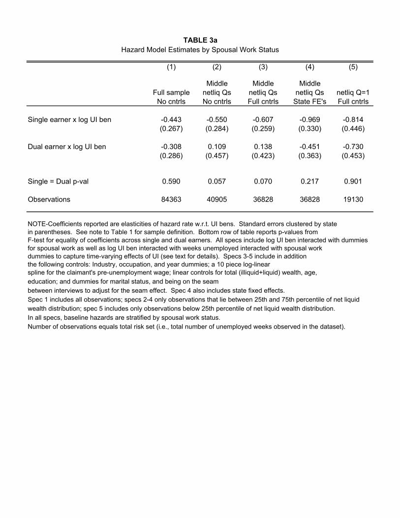
(1) (2) (3) (4) (5)

Middle Middle MiddleFull sample netliq Qs netliq Qs netliq Qs netliq Q=1

No cntrls No cntrls Full cntrls State FE's Full cntrls

-0.443 -0.550 -0.607 -0.969 -0.814(0.267) (0.284) (0.259) (0.330) (0.446)

-0.308 0.109 0.138 -0.451 -0.730(0.286) (0.457) (0.423) (0.363) (0.453)

0.590 0.057 0.070 0.217 0.901

84363 40905 36828 36828 19130

NOTE-Coefficients reported are elasticities of hazard rate w.r.t. UI bens. Standard errors clustered by statein parentheses. See note to Table 1 for sample definition. Bottom row of table reports p-values fromF-test for equality of coefficients across single and dual earners. All specs include log UI ben interacted with dummies for spousal work as well as log UI ben interacted with weeks unemployed interacted with spousal work dummies to capture time-varying effects of UI (see text for details). Specs 3-5 include in additionthe following controls: Industry, occupation, and year dummies; a 10 piece log-linear spline for the claimant's pre-unemployment wage; linear controls for total (illiquid+liquid) wealth, age, education; and dummies for marital status, and being on the seambetween interviews to adjust for the seam effect. Spec 4 also includes state fixed effects. Spec 1 includes all observations; specs 2-4 only observations that lie between 25th and 75th percentile of net liquidwealth distribution; spec 5 includes only observations below 25th percentile of net liquid wealth distribution.In all specs, baseline hazards are stratified by spousal work status.Number of observations equals total risk set (i.e., total number of unemployed weeks observed in the dataset).

TABLE 3aHazard Model Estimates by Spousal Work Status

Single earner x log UI ben

Dual earner x log UI ben

Single = Dual p-val

Observations

(1) (2) (3) (4)

Full sample Full sample Full sample netliq Q <=2No cntrls Full cntrls State FE's Full cntrls

No mortgage x log UI ben 0.269 0.322 0.263 -0.135(0.292) (0.218) (0.455) (0.390)

Mortgage x log UI ben -0.976 -0.938 -0.957 -1.552(0.424) (0.419) (0.484) (0.667)

No mortg. = Mortg. p-val 0.002 0.005 0.008 0.047

Observations 37087 35291 35291 16656

NOTE-Coefficients reported are elasticities of hazard rate w.r.t. UI bens. Standard errors clustered by statein parentheses. Sample consists of households in core sample for whom pre-unemp mortgage data is available. See note to Table 1 for definition of core sample. Bottom row of table reports p-values from F-test for equalityof coefficients across non-mortgage and mortgage holders. All specs include log UI ben interacted with mortgage dummies as well as log UI ben interacted with weeks unemployed interacted with mortgage dummies to capture time-varying effects of UI (see text for details). Specs 2-4 include in additionthe following controls: Industry, occupation, and year dummies; a 10 piece log-linear spline for the claimant's pre-unemployment wage; linear controls for total (illiquid+liquid) wealth, age, education; and dummies for marital status, spousal work, and being on the seambetween interviews to adjust for the seam effect. Spec 3 also includes state fixed effects. Specs 1-3 includes all observations; spec 4 only observations that lie below 50th percentile of net liquidwealth distribution. In all specs, baseline hazards are stratified by mortgage dummy.Number of observations equals total risk set (i.e., total number of unemployed weeks observed in the dataset).

TABLE 3bHazard Model Estimates by Mortgage Holding Status

Median pre-unemp job tenure (years) 1.9 1.6 4.8Median pre-unemp annual wage $20,828 $19,183 $29,874

Percent dropouts 14% 16% 6%Percent college grads 17% 13% 34%Percent married 58% 56% 68%Mean age 36.4 35.5 40.6Mean number of persons in hhold 2.21 2.24 2.04

NOTE--Data source is Study of Unemployment Insurance Exhaustees and Pennsylvania Reemployment Bonus Demonstration (Mathematica surveys matched to administrative UI records). These datasets are publicly available through the Upjohn Institute. All monetary values are in real 1990 dollars. Sample includes prime-age male UI claimants who are not on temporary layoff.Sample size is 2,730 observations. Data is reweighted using sampling probabilities to yield estimates for arepresentative sample of job losers. Pre-unemp job tenure is defined as number of years spent working at firm from which worker was laid off.

(0.82) (0.18)

TABLE 4Summary Statistics for Mathematica Sample

Pooled No Severance Severance

(1) (2) (3) (4)Tenure Control Full Controls Tenure Control Full Controls

Severance Pay Dummy -0.115 -0.127(0.030) (0.035)

(Netliq < Median) x Sev Pay -0.476 -0.445(0.084) (0.093)

(Netliq > Median) x Sev Pay 0.068 0.058(0.058) (0.060)

Equality of coeffs p-val <0.001 <0.001

Observations 2730 2426 2561 2426

NOTE-Coefficients reported are elasticities of hazard rate w.r.t. UI bens. Standard errors clustered bystate in parentheses. See note to Table 4 for sample definition. Bottom row of specs 3 and 4 reportsp-values from an F-test for equality of coefficients across low and high-asset groups. Columns 1 and 3include only a linear control for tenure at pre-job loss employer in addition to reported coefficients. Columns 2 and 4 include the following controls: ten piece linear splines for wages, household income, job tenure; dummies for prior industry, occupation, race, state, and year; linear controls for age, marital status, education, and household size. Baseline hazards in specs 3-4 are stratified by Netliq < Median.Netliq < Median is an indicator variable for whether the household's predicted assets (using an equation estimated from the SIPP data; see text) are below the samplemedian. Netliq > Median is defined analogously.

TABLE 5Effect of Severance Pay on Hazard Rates

Pooled By Net Liquid Wealth

.2.4

.6.8

1Fr

actio

n U

nem

ploy

ed

0 10 20 30 40 50Weeks Unemployed

Avg. UI benefit below mean Avg. UI benefit above mean

Effect of UI Benefits on Durations: Lowest Quartile of Net WealthFigure 1a

Wilcoxon Test for Equality: p = 0.01

Mean UI benefit = $185

Mean UI benefit = $140

.2.4

.6.8

1Fr

actio

n U

nem

ploy

ed

0 10 20 30 40 50Weeks Unemployed

Avg. UI benefit below mean Avg. UI benefit above mean

Effect of UI Benefits on Durations: Second Quartile of Net WealthFigure 1b

Wilcoxon Test for Equality: p = 0.04

NOTE–Sample for both figures consists of observations in the core SIPP sample for whichpre-unemployment wealth data are available. See Table 1 for definition of core sample and definitionof net liquid wealth. Figure 1a includes households in lowest quartile of real net liquid wealth. Figure1b includes those in second quartile. Each figure plots Kaplan-Meier survival curves for two groups ofindividuals: Those in state/year pairs with average weekly benefit amounts (WBA) below the samplemean and those in state/year pairs with WBAs above the mean. Survival curves are adjusted for seameffect by fitting a Cox model and recovering baseline hazards as described in text.

.2.4

.6.8

1Fr

actio

n U

nem

ploy

ed

0 10 20 30 40 50Weeks Unemployed

Avg. UI benefit below mean Avg. UI benefit above mean

Effect of UI Benefits on Durations: Third Quartile of Net WealthFigure 1c

Wilcoxon Test for Equality: p = 0.74

.2.4

.6.8

1Fr

actio

n U

nem

ploy

ed

0 10 20 30 40 50Weeks Unemployed

Avg. UI benefit below mean Avg. UI benefit above mean

Effect of UI Benefits on Durations: Highest Quartile of Net WealthFigure 1d

Wilcoxon Test for Equality: p = 0.43

NOTE–These figures are constructed in the same way as Figures 1a-b using observations in the thirdand fourth quartiles of net wealth. See notes to Figures 1a-b for details.

.2.4

.6.8

1Fr

actio

n U

nem

ploy

ed

0 10 20 30 40 50Weeks Unemployed

Avg. UI benefit below mean Avg. UI benefit above mean

Effect of UI Benefits on Durations: Single-Earner HouseholdsFigure 2a

Wilcoxon Test for Equality: p = 0.00

.2.4

.6.8

1Fr

actio

n U

nem

ploy

ed

0 10 20 30 40 50Weeks Unemployed

Avg. UI benefit below mean Avg. UI benefit above mean

Effect of UI Benefits on Durations: Dual-Earner HouseholdsFigure 2b

Wilcoxon Test for Equality: p = 0.37

NOTE–Figure 2a includes households in the core SIPP sample with one earner in the month prior tojob loss. Figure 2b includes households with two earners. See Table 1 for definition of core sample.Each figure plots Kaplan-Meier survival curves for two groups of individuals: Those in state/year pairswith average weekly benefit amounts (WBA) below the sample mean and those in state/year pairs withWBAs above the mean. Survival curves are adjusted for seam effect by fitting a Cox model andrecovering baseline hazards as described in text.

.2.4

.6.8

1Fr

actio

n U

nem

ploy

ed

0 10 20 30 40 50Weeks Unemployed

Avg. UI benefit below mean Avg. UI benefit above mean

Effect of UI Benefits on Durations: Households with MortgagesFigure 3a

Wilcoxon Test for Equality: p = 0.01

.2.4

.6.8

1Fr

actio

n U

nem

ploy

ed

0 10 20 30 40 50Weeks Unemployed

Avg. UI benefit below mean Avg. UI benefit above mean

Effect of UI Benefits on Durations: Households without MortgagesFigure 3b

Wilcoxon Test for Equality: p = 0.31

NOTE–These figures are constructed in the same way as Figures 2a-b. Figure 3a includes householdswho make mortgage payments; 3b includes all others. Only observations with mortgage data prior tojob loss are included. See notes to Figures 2a-b for additional details on construction of these figures.

.2.4

.6.8

1Fr

actio

n U

nem

ploy

ed

0 10 20 30 40 50Weeks Unemployed

Placebo Test: Effect of UI Benefits on Low-Wealth Non-RecipientsFigure 4

Avg. UI benefit below mean Avg. UI benefit above mean

Wilcoxon Test for Equality: p = 0.53

NOTE–The sample for this figure consists of prime-age male job losers in the SIPP data who (a) do notreport receiving UI benefits while unemployed, (b) report searching for a job, (c) are not on temporarylayoff, (d) have at least 3 months of wage history prior to job loss, and (e) have below-median net liquidwealth prior to job loss. Kaplan-Meier survival curves are plotted for two groups of individuals: Those instate/year pairs with average weekly benefit amounts (WBA) below the sample mean and those instate/year pairs with WBAs above the mean. Survival curves are adjusted for seam effect by fitting aCox model and recovering baseline hazards as described in text.

.4.6

.81

Frac

tion

Une

mpl

oyed

0 5 10 15 20 25Weeks Unemployed

Received Severance Pay No Severance Pay

Effect of Severance Pay on DurationsFigure 5

Wilcox Test for Equality: p = 0.00

NOTE–Data are from Mathematica surveys matched to administrative UI records. See note to Table 4for additional details on data and sample definition. Data is reweighted using sampling probabilities toyield estimates for a representative sample of job losers. Kaplan-Meier survival curves are plotted fortwo groups of individuals: Those who received a severance payment at the time of job loss and thosewho did not. Survival curves are adjusted for the effect of pre-unemployment job tenure on durations byfitting a Cox model and recovering baseline hazards as described in text.

.2.4

.6.8

1

Frac

tion

Une

mpl

oyed

0 5 10 15 20 25Weeks Unemployed

Received Severance Pay No Severance Pay

Effect of Severance Pay on Durations: Below Median Net WealthFigure 6a

Wilcox Test for Equality: p = 0.00

.2.4

.6.8

1

Frac

tion

Une

mpl

oyed

0 5 10 15 20 25Weeks Unemployed

Received Severance Pay No Severance Pay

Effect of Severance Pay on Durations: Above Median Net WealthFigure 6b

Wilcox Test for Equality: p = 0.52

NOTE–See Figure 5 for sample definition. Each of these figures is constructed in exactly the sameway as Figure 5. Figure 6a includes observations where predicted net wealth is below the samplemedian; Figure 6b includes those above the median. Net wealth is predicted using a linear function ofage, wage, education, and marital status that is estimated on the core SIPP sample as described intext.