Why Do Governments Tax or Subsidize Fossil Fuels?
72
Working Paper 541 August 2020 Why Do Governments Tax or Subsidize Fossil Fuels? Abstract Governments have long faced pressure to address the climate crisis by increasing taxes on fossil fuels, which are the source of more than three-quarters of the world’s anthropogenic carbon pollution. Since fossil fuel taxes and subsidies are hard to measure, it is unclear how much government policies have changed. Using original high-frequency data on gasoline taxes and subsidies in 157 countries, we establish three findings: despite rising alarm about climate change, from 2003 to 2015 there was little net change in fuel taxes and subsidies at a global level; fuel taxes and subsidies appear to be driven by slow-moving economic factors, primarily income and fossil fuel wealth; and reforms, when they occur, are overwhelmingly associated with country-level political conditions that follow no readily-discernible patterns. These patterns are consistent with a model in which fossil fuel taxes are determined by a country’s income and revenue needs, not its environmental commitments. www.cgdev.org Paasha Mahdavi, Cesar B. Martinez-Alvarez, and Michael L. Ross Keywords: Gasoline taxes, carbon taxes, fossil fuel subsidies, tax reform, climate policy, environmental politics, political economy JEL: H23, Q35, Q38, Q54, Q5
Transcript of Why Do Governments Tax or Subsidize Fossil Fuels?

Working Paper 541 August 2020
Why Do Governments Tax or Subsidize Fossil Fuels?
Abstract
Governments have long faced pressure to address the climate crisis by increasing taxes on fossil fuels, which are the source of more than three-quarters of the world’s anthropogenic carbon pollution. Since fossil fuel taxes and subsidies are hard to measure, it is unclear how much government policies have changed. Using original high-frequency data on gasoline taxes and subsidies in 157 countries, we establish three findings: despite rising alarm about climate change, from 2003 to 2015 there was little net change in fuel taxes and subsidies at a global level; fuel taxes and subsidies appear to be driven by slow-moving economic factors, primarily income and fossil fuel wealth; and reforms, when they occur, are overwhelmingly associated with country-level political conditions that follow no readily-discernible patterns. These patterns are consistent with a model in which fossil fuel taxes are determined by a country’s income and revenue needs, not its environmental commitments.
www.cgdev.org
Paasha Mahdavi, Cesar B. Martinez-Alvarez, and Michael L. Ross
Keywords: Gasoline taxes, carbon taxes, fossil fuel subsidies, tax reform, climate policy, environmental politics, political economy
JEL: H23, Q35, Q38, Q54, Q5

Center for Global Development2055 L Street NW
Washington, DC 20036
202.416.4000(f) 202.416.4050
www.cgdev.org
The Center for Global Development works to reduce global poverty and improve lives through innovative economic research that drives better policy and practice by the world’s top decision makers. Use and dissemination of this Working Paper is encouraged; however, reproduced copies may not be used for commercial purposes. Further usage is permitted under the terms of the Creative Commons License.
The views expressed in CGD Working Papers are those of the authors and should not be attributed to the board of directors, funders of the Center for Global Development, or the authors’ respective organizations.
Why Do Governments Tax or Subsidize Fossil Fuels?
Paasha MahdaviUniversity of California, Santa Barbara
Cesar B. Martinez-AlvarezUniversity of California, Los Angeles
Michael L. RossUniversity of California, Los Angeles
We thank Thomas Hale, Chad Hazlett, Robert Keohane, Daniel Treisman, and the participants at the February 2020 Balzan Workshop on Climate Change Politics for valuable suggestions. Our data collection efforts were generously supported by the UCLA Burkle Center and the Natural Resources Governance Institute. Earlier versions of this paper were presented at the 2018 meeting of the American Political Science Association, and seminars at University of Wisconsin, University of Colorado, University of Virginia, the UCLA Burkle Center, and the Center for Global Development, and were greatly improved by the suggestions of participants.
Mahdavi, Martinez-Alvarez, and Ross, 2020. “Why Do Governments Tax or Subsidize Fossil Fuels?.” CGD Working Paper 541. Washington, DC: Center for Global Development. https://www.cgdev.org/publication/why-do-governments-tax-or-subsidize-fossil-fuels

1 Introduction
We are remarkably ignorant about what governments are doing to address the most im-
portant challenge of the 21st century. The gravity of the climate change problem has been
widely-acknowledged by most governments since the mid-1990s.1 Yet, most studies that seek to
explain – or even describe – climate change policies are limited to one or several countries. There
are relatively few cross-national studies, and most cover the advanced industrialized democra-
cies but not the rest of the world (Battig and Bernauer, 2009; Bayer and Urpelainen, 2016; Aklin
and Urpelainen, 2013; Purdon et al., 2015; Mildenberger, 2020; Ward and Cao, 2012; Finnegan,
2019).
In part, this reflects the challenge of identifying policies that are equally salient in a wide
range of settings: the most appropriate policies vary widely, depending on a country’s geographic
characteristics, economic structure, and level of development. Hence measuring a government’s
“mitigation efforts” in ways that are comparable across countries and over time has been a
major stumbling block for researchers and policy architects alike (O’Neill et al., 2013; Aldy
et al., 2016; Bernauer and Bohmelt, 2013). For some scholars, the measurement problem is so
intractable that “the quest to find a single cause, or even a common set of drivers, to explain
climate leaders or climate laggards is a near-futile exercise” (Christoff and Eckersley, 2011).
Our approach is to focus on policies that encourage or discourage the use of fossil fuels,
which since 2000 have been the source of about 78 percent of all anthropogenic greenhouse
gas pollution (Clarke and (coord. lead authors), 2015). We concentrate on transportation
fuels, which generate about 23 percent of global energy-related emissions (Sims, 2014). All
governments have policies that encourage or discourage the consumption of transportation fuels,
typically through a complex web of policies that have the effect of taxing or subsidizing the retail
price. These varied policies have led to remarkable country-to-country differences in prices: in
June 2020, a liter of gasoline sold for $0.02 in Venezuela and $2.24 in Hong Kong.2
Taxes and subsidies for fossil fuels have profound consequences: they affect fuel consumption
(Charap et al., 2013; Fattouh and El-Katiri, 2013), greenhouse gas pollution (Erickson et al.,
1Since the mid-1990s, almost all countries have been members of the United Nations Framework Conventionon Climate Change (UNFCCC), whose stated objective is to stabilize greenhouse gas concentrations “at a levelthat would prevent dangerous anthropogenic interference with the climate system.”
2Globalpetrolprices.com, accessed June 26, 2020.
1

2020), investments in renewable energy (Aghion et al., 2016), inequality (Del Granado et al.,
2012), and the fiscal health of governments. They also affect political stability: between 2006
and 2019, attempts to raise gasoline prices were followed by protests in at least 24 countries.3
The 1999 overthrow of Indonesia’s Suharto government, Myanmar’s 2007 “Saffron Rebellion,”
and France’s 2018-19 “Gilets jaune” movement all began as protests against higher gasoline
prices. As Ansolabehere and Konisky (2014, 17) note, “people are acutely aware of energy
prices.”
There is strong international support for removing subsidies and raising taxes on fossil fuels.
The Intergovernmental Panel on Climate Change (IPCC) describes the removal of fossil fuel
subsidies as one of the simplest and cheapest ways for countries to curtail carbon pollution
(Sims, 2014). Other international institutions – including the World Bank, the International
Monetary Fund, the United Nations Environmental Program, and the International Energy
Agency – have also urged governments to abolish these subsidies (McFarland and Whitley,
2014). Many governments nominally support fuel price reforms: in September 2009, the G20
heads of state agreed to phase out “inefficient fossil fuel subsidies,” while the 21 governments
of the Asia Pacific Economic Cooperation group made a similar vow (McFarland and Whitley,
2014). In June 2010, nine additional governments formed the “Friends of Fossil Fuel Subsidy
Reform” to support these efforts.
Despite these initiatives, fossil fuel taxes and subsidies can be remarkably hard to change.
The federal gasoline tax in the US was last changed in 1994. More recent efforts to reduce
subsidies in Angola, Mexico, Nigeria, Indonesia, Sudan, Egypt, Azerbaijan, and Venezuela have
all been rolled back or nullified by falling exchange rates or rising inflation. As a result, fossil
fuel subsidies remain large: depending on how they are measured, they are worth between $500
billion and $5.2 trillion dollars a year (Kojima and Koplow, 2015; Coady et al., 2017). After
falling in 2015 and 2016, they rose in 2017 and 2018, returning to their 2014 levels (Matsumura
and Zakia, 2019).
Cross-national research on the politics of fossil fuel taxes and subsidies has been limited,
partly because data have been scarce. As a result, previous analyses have been based on either
compilations of case studies (e.g., Inchauste and Victor, 2017; Skovgaard and van Asselt, 2018;
Clements et al., 2013), or a public data set that measures prices at two-year intervals, and hence
3See Appendix Table S3 for a list of countries, dates and sources.
2

tells us relatively little about the frequency and timing of reforms (Cheon et al., 2013; Wagner,
2013).
We compile an original data set on the monthly value of gasoline taxes and subsidies in 157
countries from 2003 to 2015, totaling 23,550 observations. Using these data we estimate the
relationship between fuel taxes and a wide range of potentially-salient economic and political
factors.
We find three robust patterns. First, fuel taxes and subsidies are highly resistant to change.
Despite thirteen years of rising alarm about greenhouse gas emissions, there was little net change
in fuel taxes and subsidies over the 2003-15 period. Fuel taxes rose modestly in 73 countries,
fell modestly in 63 countries, and were unchanged in five. On average, countries raised their
per-liter gasoline taxes by 2.05 percent per year. Yet this fails to capture the global trend, since
consumption fell in high-tax countries but rose in low-tax countries. If we weight each country
to reflect its annual gasoline consumption, per-liter gas taxes fell globally by 5.43 percent per
year. In short, governments collectively made little progress toward raising taxes on gasoline
and diesel fuel.
Second, fuel tax and subsidy levels are strongly associated with the same three factors that
drive other types of taxes: income per capita, which is linked to disposable income, the demand
for public goods, and the size of government (Ortiz-Ospina and Roser, 2020; Akitoby et al., 2006;
Drazen, 2004; Luttmer and Singhal, 2011); government debt, which is associated with higher
taxes (Schneider and Heredia, 2003); and oil and gas wealth, which provides an alternative
source of government revenues and tends to reduce other types of taxes (Prichard et al., 2018;
Brautigam et al., 2008). All three factors change slowly, and may help keep fuel taxes and
subsidies in place through what Victor (2009, 7) calls “a political logic that is often difficult to
alter.”
Finally, the small changes in fuel taxes that did occur were primarily associated with unob-
served, time-varying, country-specific factors. This result stands in contrast with prior studies
that suggest governments adopt more climate-friendly policies when they are more democratic
(Cheon et al., 2013; Midlarsky, 1998; Neumayer, 2002; Bayer and Urpelainen, 2016); when they
have more effective bureaucracies, which can compensate the losers from environmental reforms
(Kyle, 2018; Cheon et al., 2013; Victor, 2009); or when elections or leadership changes create
3

“windows of opportunity” (Moerenhout, 2018; Harrison and Sundstrom, 2007).
We find no support for these or other arguments about the role of political factors. Instead,
our analysis supports recent qualitative research on fuel tax reform that emphasize the impor-
tance of each country’s unique configurations of actors, events, constraints and opportunities
(Clements et al., 2013; Skovgaard and van Asselt, 2018; Inchauste and Victor, 2017; Rabe,
2018).
In sum, our analysis implies that fuel tax policies are determined by slowly-moving macro-
level economic conditions, while changes in these policies are largely a function of micro-level
political conditions that are highly context-specific. Our results are robust to many alternative
specifications and the use of instrumental variables for fossil fuel wealth.
To explain these results, we argue they are consistent with a model in which fuel taxes are
first and foremost taxes, not instruments of environmental policy. As such, they are jointly
driven by a government’s demand for revenues and the public’s willingness to supply them;
these in turn are affected by a country’s income, debt, and natural resource endowment. When
there is a gap between the fuel taxes that a government seeks to impose and the amount that
citizens are willing to pay, the outcome is resolved by country-specific political factors, such as
the capacity of citizens to mobilize, and the government’s ability to curtail this mobilization.
At the broadest level, our research contributes to the study of climate change politics
(Bernauer, 2013; Hughes and Lipscy, 2013; Javeline, 2014). We make three contributions to
this literature. First, we offer a significantly improved way to measure the actions that govern-
ments are taking to curb greenhouse gas emissions. Unlike other climate policy indicators, our
measure of monthly fossil fuel taxes and subsidies does not rely on subjective judgments; it only
records implemented policies, not nominal ones; and it allows researchers to make fine-grained
comparisons of policies across countries and over time. To the best of our knowledge, our data
offers the most accurate and fine-grained measure of an important climate policy for a large
number of countries over a significant period of time.
Second, we provide new insights about global progress on taxing carbon fuels. The concept
of taxing carbon fuels has received widespread support among policy analysts, yet the success
of these efforts has been difficult to measure. Our analysis covers the thirteen-year period
leading up to the 2015 Paris Accord, which was characterized by growing alarm about the
4

consequences of global climate change, and heightened international support for both reducing
subsidies and raising taxes on fossil fuels. We find that over this period, taxes on one category of
fossil fuels – transportation fuels – did not significantly increase, and by one measure, actually
decreased. We take this as evidence of how difficult it is for governments to raise the cost of
carbon fuels, and how a different political imperative – funding the government while avoiding
protests – typically takes precedence. Less contentious emissions-reduction strategies – like
making renewable energy cheaper, curtailing fossil fuel use through standards instead of prices,
and encouraging subnational political action – may ultimately be more effective.
Finally, we suggest a new perspective on the global politics of fuel taxes: that they are
mostly determined by the revenue needs of governments and largely unresponsive to the climate
catastrophe. If these patterns hold for other types of carbon policies – a question we do not
try to answer here – they may deepen our understanding of the political economy of climate
change, and cast light on general patterns, obstacles, and opportunities.
We also bring several innovations to the study of fossil fuel taxes and subsidies.4 Most
research on this topic has been based on in-depth, highly granular, qualitative case studies;
quantitative analyses have lagged behind, in part because of limited data. Our analysis is the
first to use both monthly and annual data covering a large number of countries and years, to
correct for distortions caused by broad-based taxes, to more carefully test alternative arguments,
and to address the endogeneity of natural resource wealth. These innovations give us a stronger
platform to evaluate the sources of fossil fuel taxes and subsidies.
The next section explains how we measure taxes and subsidies for gasoline and diesel, along
with other key variables. Our empirical analysis is in section three. We discuss our results in
section four, where we also develop a simple model to show how income, fossil fuel dependence,
and local politics can account for the observed patterns. Section five concludes.
4Throughout this paper we use the terms “fossil fuel taxes” and “gasoline taxes” to refer to both taxes andsubsidies. Subsidies can be characterized as negative taxes.
5

2 Data
2.1 Gasoline Taxes
To measure taxes and subsidies for gasoline, we collected data on local retail gas prices from
January 2003 to June 2015 for 157 countries, representing 97.1% of the world’s population and
accounting for 98.2% of all greenhouse gas emissions. The countries included all sovereign states
with populations over one million in 2012, except for four countries where we failed to obtain
reliable data (Cuba, Eritrea, North Korea, and Turkmenistan).5 Data are missing for 1,067 (4.5
percent) of the 23,550 country-months. Appendix Section 1 explains our method for deriving
taxes and subsidies, the full list of countries and months (Table S1), and describes our data
sources (Table S2).6
There are several ways to define and measure fossil fuel taxes and subsidies. We use a
conservative definition and employ the “price gap” method.7 Since refined petroleum products
are traded internationally, it is possible to calculate the international supply cost – that is, the
cost of bringing a liter of gasoline or diesel to consumers. Since they are sold on retail markets
in virtually all countries, their in-country prices are observable. The difference between the
international supply cost and the local retail price is the price gap and constitutes the implicit
fuel tax or subsidy (Koplow, 2009).
We also correct for the effects of any general sales taxes, such as value-added taxes (VAT),
that are imposed on all goods and services. Because they do not affect the price of gasoline
or diesel relative to other goods, general sales taxes cannot cause consumers to switch toward
cheaper transportation alternatives. We therefore control for the effects of VAT and other
broadly-applied sales taxes with a novel data set created by the International Monetary Fund.8
Our measure of fossil fuel taxes and subsidies has three valuable properties. First, it tell us
5Over a three-year period, our research team gathered data from a large number of primary and secondarysources, working in ten languages. In 17 countries, we employed local researchers to obtain primary data thatwere not otherwise accessible.
6For the separate analysis of diesel taxes and subsidies, we use the biannual observations from Wagner (2013).7The IMF identifies two classes of petroleum subsidies: “pre-tax subsidies,” which represent the difference
between the retail price and the international supply cost, and “post-tax subsidies” which are defined as thedifference between the retail price and the sum of the supply cost, a basic consumption tax, and a Pigouvian taxthat offsets the costs of local pollution, congestion, and carbon emissions (Coady et al., 2017). Post-tax subsidiesare, by construction, larger than pre-tax subsidies. We only examine pre-tax subsidies.
8While the VAT correction makes our estimates more precise, it does not affect any of our results, which aresubstantially unchanged when the VAT correction is dropped.
6
about a policy that is politically costly to adopt. When climate policies are uncontroversial, their
adoption tells us relatively little about the depth of the government’s policy commitments. But
the price of fuel affects many citizens on a daily level, and policies that raise it can be politically
risky and lead to protest. This makes it a useful way to gauge a government’s capacity to sustain
carbon-reducing policies that raise consumer costs.
Second, it reveals the taxes and subsidies that were implemented, not merely ones that
were publicly announced. Many governments declare ambitious climate policies that they fail
to implement; others will adopt costly reforms without announcing them. We only measure
policies once they affect prices at the pump.
Finally, our measure captures the size of the net tax or subsidy. A wide range of government
policies can affect fossil fuels at different points in the supply chain – taxing or subsidizing the
extraction, import, refining, or transportation of fuel – in ways that ultimately affect the retail
price. Governments can also change the retail price directly, even without making formal changes
to the tax code: state-owned oil companies, for example, can raise or lower gasoline prices by
fiat. Our indicator measures the aggregated effects of these policies, producing a more complete
picture of the consumption incentives or disincentives maintained by governments. Since some
of these price-altering policies cannot be formally classified as taxes or subsidies, we refer to our
measure as net implicit taxes and subsidies.
2.2 Explanatory variables
To learn about the correlates of fuel tax levels, we take an inductive approach. We begin with
a baseline model that includes three economic variables that are widely believed to influence
a country’s tax structure: fossil fuel endowment, income per capita, and government debt.
We then add variables to test alternative arguments about the role of democratic institutions,
bureaucratic effectiveness, elections, oil discoveries, and leadership changes. In the Appendix
we test additional arguments about the role of national oil companies and car ownership.
2.2.1 Fossil Fuel Wealth
Fossil fuel subsidies are strongly associated with oil and gas wealth, but the latter has not
been well-measured. Previous studies of fuel taxes have used OPEC membership as a proxy for
7

oil wealth, yet OPEC members produce less than 40 percent of the world’s oil and gas (Cheon
et al., 2013, 2015). A country’s fossil fuel production may also be endogenous to its fossil fuel
taxes, possibly leading to biased estimations.
We use three more fine-grained measures. Our preferred measure is Fossil Fuel Dependence,
which is the fraction of a country’s GDP that comes from oil and gas production and may be the
most intuitive way to make comparisons across countries. Our alternative measures focus on oil
exports: Fossil Fuel Exports Dependence, which expresses oil and gas exports as a fraction of
total exports, and Oil and Gas Exports per capita, which expresses these exports in per capita
terms. Although they are highly correlated, each captures a slightly different dimension of
fossil fuel abundance: countries like Chad, with low incomes and modest levels of oil wealth,
will have relatively high values of Fossil Fuel Dependence and Fossil Fuel Export Dependence
but relatively low values of Oil and Gas Exports per capita; countries like Norway, with more
diversified economies but greater per capita oil wealth, will have the opposite. We take our data
on oil and gas production and exports from Ross and Mahdavi (2015) and World Bank (2019).
To evaluate the impact of oil and gas wealth at the monthly level, we use data on giant oil field
discoveries from Arezki et al. (2017).
Since we recognize that all of the oil wealth measures may be endogenous to other variables in
our model (such as income and fuel taxes), we instrument for fossil fuel wealth using a country’s
1960 oil endowment per capita. For robustness, we also employ an alternative instrument based
on the spatial distribution of oil-yielding sedimentary basins (Cassidy, 2018). We assume that,
conditional on the revenues generated from oil production, the historical geological endowment
of a country’s oil is plausibly exogenous from present-day implicit taxes on gasoline. To protect
against violations of the exclusion restriction using this instrument, we follow Cassidy (2018) by
controlling for potential geographical correlates of geological endowments and fuel price policies,
which in our case include latitude, coastal access, and regional indicators.
2.2.2 Other variables
Our main economic measures (GNI Per Capita and Central Government Debt) are drawn
from the World Development Indicators and the International Monetary Fund (World Bank,
2019; IMF, 2019a). Our baseline measure of democracy is the Polity IV score from Marshall
8

et al. (2011), which we convert to the categorical measure Autocracy ;9 as alternatives, we also
use the Electoral Democracy score from the Varieties of Democracy database (Coppedge et al.,
2015) and a dichotomous measure of democracy from Boix et al. (2013). The Government
Effectiveness score comes from the Worldwide Governance Indicators (WGI) and measures
both expert and public perceptions of the quality of public services, the civil service, and policy
formulation and implementation (World Bank, 2019). To measure the incidence of elections
and leadership changes, we use data from the Archigos dataset (Goemans et al., 2009) and the
NELDA project (Hyde and Marinov, 2015). Value-added tax data comes from the IMF (2019b).
3 Analysis
Our analysis is exploratory and we do not make strong claims about causal inference. In-
stead, our goals are to describe changes in fuel taxes from 2003 to 2015, and determine if prior
arguments about the causes of fuel tax reform are consistent with our data. We begin with a
cross-national analysis to evaluate explanations for fuel tax levels, then analyze panel data to
evaluate explanations for policy changes. We also use biannual data on diesel prices from 2004
to 2014 from Wagner (2013) and ask similar questions about diesel taxes and subsidies.
3.1 Fuel tax levels, 2003-15
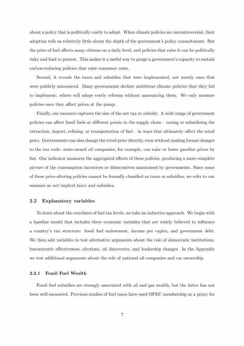
Figure 1 shows gasoline taxes and subsidies for 155 countries over the 2003-15 period.10
Each gray line represents the retail price in a single country, while the heavy red line displays
the “benchmark price,” representing the supply cost of a liter of gasoline.11 States fall into two
groups: those above the red benchmark line, whose gasoline prices are greater than the supply
cost (indicating they are taxing gas sales), and those below the benchmark line, whose prices
are less than the supply cost (indicating they are subsidizing gasoline). Of the 155 countries
in our data, 133 (85.8 percent) were net taxers for most of this period, while 22 (14.2 percent)
9Specifically, we converted the Polity IV into a binary variable denominated Autocracy that takes the valueof 1 when the Polity IV score is equal to or lower than -6, and zero otherwise.
10Although we have local price data for Myanmar and Somalia, we could not include them because they lackedmarket exchange rates for their currencies during this period.
11For the benchmark price we use the spot price for conventional refined gasoline at the New York Harbor,adjusted to account for distribution costs.
9
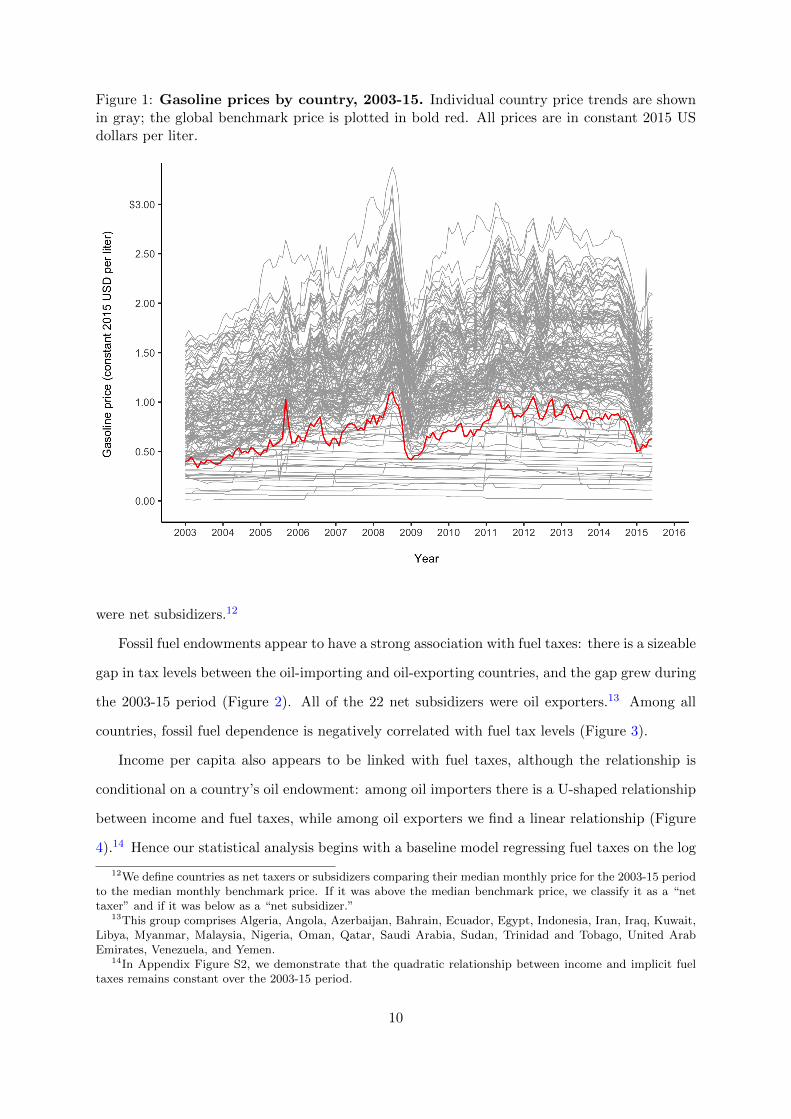
Figure 1: Gasoline prices by country, 2003-15. Individual country price trends are shownin gray; the global benchmark price is plotted in bold red. All prices are in constant 2015 USdollars per liter.
were net subsidizers.12
Fossil fuel endowments appear to have a strong association with fuel taxes: there is a sizeable
gap in tax levels between the oil-importing and oil-exporting countries, and the gap grew during
the 2003-15 period (Figure 2). All of the 22 net subsidizers were oil exporters.13 Among all
countries, fossil fuel dependence is negatively correlated with fuel tax levels (Figure 3).
Income per capita also appears to be linked with fuel taxes, although the relationship is
conditional on a country’s oil endowment: among oil importers there is a U-shaped relationship
between income and fuel taxes, while among oil exporters we find a linear relationship (Figure
4).14 Hence our statistical analysis begins with a baseline model regressing fuel taxes on the log
12We define countries as net taxers or subsidizers comparing their median monthly price for the 2003-15 periodto the median monthly benchmark price. If it was above the median benchmark price, we classify it as a “nettaxer” and if it was below as a “net subsidizer.”
13This group comprises Algeria, Angola, Azerbaijan, Bahrain, Ecuador, Egypt, Indonesia, Iran, Iraq, Kuwait,Libya, Myanmar, Malaysia, Nigeria, Oman, Qatar, Saudi Arabia, Sudan, Trinidad and Tobago, United ArabEmirates, Venezuela, and Yemen.
14In Appendix Figure S2, we demonstrate that the quadratic relationship between income and implicit fueltaxes remains constant over the 2003-15 period.
10

Figure 2: Gasoline prices 2003-15, oil exporters versus importers. Oil exporter andimporter group averages are computed monthly using unweighted country taxes and subsidies.
Figure 3: Fuel dependence and net implicit taxes by country. Cross-sectional rela-tionship between net implicit fuel taxes and fossil fuel dependence, both averaged across the2003-2015 period. Countries above 30% fossil fuel exports dependence are labeled to illustratethe high correlation (ρ = 0.84) between fuel dependence indicators.
11

Figure 4: Income per capita and net implicit taxes by country. Cross-sectional relation-ship between net implicit fuel taxes and GNI per capita, both averaged across the 2003-2015period, in oil-exporting countries (top panel) and oil-importing countries (bottom panel). Alocal smoother is shown to illustrate the approximately linear relationship in oil-exporters (thesmoother excludes Norway, which is the outlier in the upper right quadrant) versus the U-shapedrelationship in oil-importers. Model-based results plotted in Appendix Figure S1.
12

Table 1: Cross-Section / Basic Specification
Dependent variable:
Net Implicit Tax on Gasoline
(1) (2) (3) (4)
log(GNI Per Capita) −1.032∗∗∗ −0.939∗∗∗ −0.873∗∗∗ −0.745∗∗∗
(0.193) (0.181) (0.181) (0.182)log(GNI Per Capita Sq) 0.066∗∗∗ 0.061∗∗∗ 0.057∗∗∗ 0.050∗∗∗
(0.011) (0.011) (0.011) (0.011)Fossil Fuel Dependence −0.016∗∗∗
(0.004)log(Oil and Gas Exports PC) −0.024∗∗∗
(0.005)Fossil Fuel Export Dependence −0.007∗∗∗
(0.001)Central Government Debt 0.003∗∗∗ 0.002∗∗ 0.002∗∗ 0.002∗∗
(0.001) (0.001) (0.001) (0.001)Value-Added Tax Rate 0.049∗∗∗ 0.042∗∗∗ 0.041∗∗∗ 0.035∗∗∗
(0.005) (0.005) (0.005) (0.005)Constant 3.543∗∗∗ 3.328∗∗∗ 2.986∗∗∗ 2.695∗∗∗
(0.817) (0.750) (0.750) (0.747)
Observations 140 139 139 136R2 0.598 0.673 0.672 0.737Adjusted R2 0.586 0.660 0.660 0.727
Note: Robust SE ∗p<0.1; ∗∗p<0.05; ∗∗∗p<0.01
of income per capita and the square of logged income, fossil fuel dependence, and government
debt. We also include VAT as a control (Table 1).
The estimates are consistent with the scatterplots: there is a quadratic relationship between
GNI per capita and fuel taxes, (Table 1, column 1; see also Appendix Figure S1), a negative
relationship between Fossil Fuel Dependence and fuel taxes (Table 1, column 2), as well as a
positive relationship between Central Government Debt and fuel taxes. When we measure fossil
fuel endowments in alternative ways (Table 1, columns 3 and 4), the R-squared term is similar
or larger. The R-squared terms in columns 2-4 suggest these variables account for between 67%
and 74% of the variation in fuel taxes.15
In Table 2 we evaluate two political factors: Autocracy and Government Effectiveness.
We also include an interaction term for Fossil Fuel Dependence and the Autocracy dummy, to
investigate the claim that oil-rich autocracies are unusually reliant on fossil fuel subsidies, which
15Without the VAT-adjustment, GNI per capita and Fossil Fuel Dependence account for between 42% and57% of the variation; the F -statistic for models with and without VAT is 97.4, indicative of the need for VAT-adjustment.
13

Table 2: Cross-Section / Additional Controls
Dependent variable:
Net Implicit Tax on Gasoline
(1) (2) (3) (4)
log(GNI Per Capita) −0.939∗∗∗ −0.957∗∗∗ −0.957∗∗∗ −0.519∗∗
(0.181) (0.194) (0.194) (0.207)log(GNI Per Capita Sq) 0.061∗∗∗ 0.061∗∗∗ 0.061∗∗∗ 0.036∗∗∗
(0.011) (0.012) (0.012) (0.013)Fossil Fuel Dependence −0.016∗∗∗ −0.015∗∗∗ −0.015∗∗∗ −0.016∗∗∗
(0.004) (0.005) (0.005) (0.005)Central Government Debt 0.002∗∗ 0.002∗∗ 0.002∗∗ 0.001∗
(0.001) (0.001) (0.001) (0.001)Autocracy (Polity IV) −0.108 −0.108 −0.032
(0.102) (0.102) (0.103)Fossil Fuel Dependence * Autocracy 0.001 0.001 0.002
(0.008) (0.008) (0.006)Government Effectiveness 0.045 0.045 0.013
(0.078) (0.078) (0.080)European Union −0.092
(0.122)Latitude 0.001
(0.001)Landlocked 0.003
(0.054)Asia + Pacific −0.064
(0.104)Europe + North America 0.039
(0.171)Former USSR −0.333∗∗
(0.139)Latin America + Caribbean −0.248∗∗∗
(0.089)Middle East −0.369∗∗∗
(0.121)Value-Added Tax Rate 0.042∗∗∗ 0.042∗∗∗ 0.042∗∗∗ 0.038∗∗∗
(0.005) (0.005) (0.005) (0.008)Constant 3.328∗∗∗ 3.485∗∗∗ 3.485∗∗∗ 1.770∗∗
(0.750) (0.771) (0.771) (0.831)
Observations 139 134 134 134R2 0.673 0.709 0.709 0.766Adjusted R2 0.660 0.690 0.690 0.735
Note: Robust SE ∗p<0.1; ∗∗p<0.05; ∗∗∗p<0.01
they use to maintain popular support (Ross, 2012; Fails, 2019). We show in Appendix Table S4
that there is an unconditional, bivariate correlation between each of the “democracy” measures
and fuel taxes. But when we place each of the measures in the full model, none are statistically
correlated with fuel taxes and their inclusion has little effect on the baseline results.16 Adding
16The failure to find heterogeneous effects is illustrated in Appendix Figure S3.
14

a series of regional controls to the model, plus measures of geography (latitude and coastal
access), raises the R-squared and reduces the size of the GNI per capita and GNI per capita
squared coefficients but otherwise does not change these results (column 4).
In the Appendix, we show that these results are unchanged when we use alternative measures
for democracy (Tables S5–S6) and regional categories (Table S7); when we control for the
presence of national oil companies (Table S8), a factor highlighted by Cheon et al. (2015); and
when we control for the number of cars per capita (Table S9), which plausibly represents the
size of the constituency benefiting directly from fuel subsidies.
These results could be biased by the endogeneity of Fossil Fuel Dependence to both our
outcome and several of the other right-hand side variables (GNI per capita, Autocracy, and
Government Effectiveness).17 In Table 3, we show results from two-stage least squares models
in which we use a country’s 1960 oil endowment per capita to instrument for Fossil Fuel De-
pendence. The data comes from Tsui (2011), cited by Cassidy (2018). See Table S11 for results
from first-stage models.
The instrument produces no change in the statistical significance of Fossil Fuel Dependence
or the other right-hand side variables, although it causes the instrumented Fossil Fuel Depen-
dence coefficients to roughly double in size, implying an attenuation bias in the naıve model
using the endogenous regressor. To further check our results, we use an alternative instrument
for Fossil Fuel Dependence, based on the spatial distribution of oil-yielding sedimentary basins
and taken from Cassidy (2018) (Table S10). While the instrument is less efficient—the first
stage F statistic is 17 compared to an F of 283 for the endowment instrument (Table S11)—the
results are substantively similar.
17On the problem of endogeneity in the political effects of oil wealth, see, for example, Haber and Menaldo(2011).
15

Table 3: Instrumental Variables Approach
Dependent variable:
Net Implicit Tax on Gasoline
(1) (2) (3) (4)
log(GNI Per Capita) −0.869∗∗∗ −1.041∗∗∗ −1.041∗∗∗ −0.519∗∗
(0.205) (0.212) (0.212) (0.235)log(GNI Per Capita Sq) 0.058∗∗∗ 0.072∗∗∗ 0.072∗∗∗ 0.044∗∗∗
(0.012) (0.014) (0.014) (0.015)Fossil Fuel Dependence −0.032∗∗∗ −0.033∗∗∗ −0.033∗∗∗ −0.033∗∗∗
(0.005) (0.006) (0.006) (0.007)Central Government Debt 0.001 0.001 0.001 0.001
(0.001) (0.001) (0.001) (0.001)Autocracy (Polity IV) −0.165 −0.165 −0.080
(0.148) (0.148) (0.145)Fossil Fuel Dependence * Autocracy 0.010 0.010 0.009
(0.009) (0.009) (0.008)Government Effectiveness −0.122 −0.122 −0.150∗
(0.086) (0.086) (0.088)European Union −0.168
(0.115)Latitude 0.002
(0.002)Landlocked −0.026
(0.068)Asia + Pacific −0.133
(0.104)Europe + North America −0.113
(0.172)Former USSR −0.467∗∗∗
(0.167)Latin America + Caribbean −0.374∗∗∗
(0.105)Middle East −0.411∗∗∗
(0.129)Value-Added Tax Rate 0.034∗∗∗ 0.040∗∗∗ 0.040∗∗∗ 0.041∗∗∗
(0.005) (0.005) (0.005) (0.006)Constant 3.230∗∗∗ 3.527∗∗∗ 3.527∗∗∗ 1.383
(0.852) (0.842) (0.842) (0.957)
Observations 137 132 132 132Adjusted R2 0.587 0.633 0.633 0.684
Note: Robust SE ∗p<0.1; ∗∗p<0.05; ∗∗∗p<0.01
16

3.2 Changes in Fuel Taxes
How much did fuel taxes change from 2003 to 2015? What caused the changes?
In Figure 5 we display how fuel taxes changed for the 141 countries with relatively complete
data for both 2003 and 2015. The x-axis shows the implicit tax or subsidy in the first six months
of 2003, while the y-axis shows the implicit tax or subsidy for the first half of 2015. Over these
13 years, taxes rose modestly in 73 countries (51.8 percent), fell modestly in 63 countries (44.7
percent), and were unchanged in five (3.5 percent). Countries were almost as likely to reduce
taxes as to raise them.18
If we weight all countries equally, the median gasoline tax rose from $0.29 per liter to
$0.37 per liter between 2003 and 2015; this is equivalent to an annual increase of 2.05 percent,
adjusted for inflation. We can alternatively weight each country’s price by its gasoline con-
sumption in the same year, giving high-consuming countries more weight than low-consuming
countries. The median consumption-weighted tax fell from $0.12 to $0.06 per liter – a drop
of 48.8 percent, equivalent to an annual decline of 5.43 percent.The downward trend in the
consumption-weighted price reflects a global shift: while consumption fell among the high-tax
countries (which were generally high-income, oil-importing states), it rose among low-tax coun-
tries (which were predominantly middle-income and oil-exporting states).
We report a similar pattern for diesel fuel: from 2004 to 2014, the unweighted median diesel
tax rose from $0.22 per liter to $0.25 per liter, a total-period increase of 12.0 percent and an
annual increase of just 0.95 percent.19 Diesel taxes rose in 62 countries and fell in 66 countries.
For many issues, the absence of global policy change might be unremarkable. But the
absence of change in fossil fuel taxes and subsidies from 2003 to 2015 is surprising, since this
was a period of rapidly-growing attention to both the hazards of climate change and the benefits
of taxing carbon emissions.
Table 4 displays the results from a fixed-effects model with our monthly fuel tax data
aggregated into annual observations.20 As with the cross-country results, Fossil Fuel Dependence
18These trends are not sensitive to the choice of beginning and end dates: when we use the second half of2003 and the second half of 2014 as alternative beginning and end periods, the trends are similar.
19We are unable to perform a consumption-weighted calculation for diesel given the lack of time-series dataon country-level diesel consumption.
20Note we choose the fixed-effects specification as we are interested in within-country changes over time. InAppendix Tables S12–S15, we also show the results from a pooled model without fixed effects.
17

Figure 5: Gasoline taxes by country in 2003 and 2015. This figure compares the averageper-liter tax or subsidy for countries in the first six months of 2003 to the first six months of2015. Taxes or subsidies are net of each country’s value-added tax rate; this is calculated asPriceit ∗ (1 − V ATit) − Benchmarkt. Countries with the same level of taxes or subsidies inboth periods will fall along the 45-degree dashed line. Countries with higher taxes (or lowersubsidies) in 2015 than in 2003 are colored in blue; those with lower taxes (or higher subsidies)are colored in dark orange. See also Appendix Figures S4–S5.
is negatively associated with fuel taxes, even after accounting for country and year fixed effects.
Both Central Government Debt and VAT remain statistically correlated with fuel taxes, but
GNI per capita does not. Government Effectiveness continues to be uncorrelated with fuel
taxes. Autocracy is statistically associated with fuel taxes at the 10% level, but the sign on
the coefficient is reversed from the model in Table 2. Further, there remains no evidence of a
differential effect of fuel dependence on taxes between autocracies and democracies.
A model with only country-fixed effects and no other covariates gives an adjusted R2 of
0.915, indicating that the overwhelming majority of the variation in our data is cross-sectional,
18

Table 4: Cross-section Time-series: Annual Panel
Dependent variable:
Net Implicit Tax on Gasoline
log(GNI Per Capita) −0.020(0.097)
log(GNI Per Capita Sq) 0.004(0.006)
Fossil Fuel Dependence −0.006∗∗∗
(0.002)Central Government Debt 0.001∗∗∗
(0.0003)Autocracy (Polity IV) 0.096∗
(0.054)Fossil Fuel Dependence * Autocracy −0.005
(0.003)Government Effectiveness 0.026
(0.031)Value-Added Tax Rate 0.018∗∗∗
(0.004)Constant 0.147
(0.400)
Observations 1,522Country and Year FE YAdjusted R2 0.931
Note: Robust SE ∗p<0.1; ∗∗p<0.05; ∗∗∗p<0.01
not intertemporal (Figure 6).21 Our baseline model—including income, fossil fuel dependence,
debt, and VAT—accounts for about 20% of the remaining intertemporal variation (0.017/0.085
in the annual panel regressions and 0.025/0.126 in the monthly panel regressions), while the
remaining 80% is accounted for by unobserved, time-varying, country-specific factors.
Our monthly data allows us to estimate the role of three types of infra-annual events: the
discovery of giant oil fields, elections, and leadership turnover. Our dependent variable is now
the monthly measure of Net Implicit Tax on Gasoline. In Table 5 we enter each measure with
leads and lags by quarters. There appears to be no statistical relationship between fuel taxes
and the timing of elections or changes in political leadership. The month of an oil discovery
and the following two quarters are associated with higher fuel taxes at the p=.05 and p=.10
levels, albeit with a small substantive effect; this is not consistent with the notion that fossil
fuel wealth leads to reduced fuel taxes, and we cannot rule out the possibility that this result
21Adding year-fixed effects only marginally improves the fit of the model: an adjusted R-squared increase to0.922, and an F -statistic of only 13.2 (p < 0.0001).
19
Figure 6: Deviation from within-country versus across-country average net implicittax on gasoline. Each point in the graph represents the difference between a country-month-year tax and the overall country mean (x-axis) and the overall monthly mean (y-axis). The 95%quantile range of across-country deviations is roughly 3 times larger than the within-countrydeviation range; a sample with balanced across-country and within-country variation wouldhave roughly equal ranges.
is an artifact of the oil discoveries dataset, making us reluctant to draw inferences.
For each variable we tried a range of other specifications, including leads and lags to cover
events one to twelve months before, and one to twelve months following, each type of event.
The results were substantively unchanged.22
The results across these three model specifications – cross-sectional, instrumental variables
analysis, and fixed-effects panel – are plotted in Figure 7 for four of our variables of interest:
GNI per capita, Fossil Fuel Dependence, Central Government Debt, and Autocracy.
22In the Appendix, we show the results of a pooled model with monthly data (Table S16).
20

Table 5: Cross-section Time-series: Monthly Panel
Dependent variable:
Net Implicit Tax on Gasoline
1 Qr Before Elections 0.001(0.009)
2 Qr Before Elections 0.004(0.010)
3 Qr Before Elections 0.001(0.009)
4 Qr Before Elections 0.001(0.010)
1 Qr After Elections 0.002(0.009)
2 Qr After Elections −0.003(0.009)
3 Qr After Elections −0.007(0.010)
4 Qr After Elections −0.011(0.009)
1 Qr After Leader Turnover 0.010(0.015)
2 Qr After Leader Turnover 0.013(0.014)
3 Qr After Leader Turnover 0.017(0.014)
4 Qr After Leader Turnover 0.008(0.014)
Oil Discovery Month 0.041∗∗
(0.017)1 Qr After Discovery Month 0.033∗∗
(0.016)2 Qr After Discovery Month 0.026∗
(0.015)3 Qr After Discovery Month 0.016
(0.015)4 Qr After Discovery Month 0.023
(0.016)Constant 0.218∗∗∗
(0.015)
Observations 22,124Country FE YAdjusted R2 0.898
Note: Robust SE ∗p<0.1; ∗∗p<0.05; ∗∗∗p<0.01
21

Figure 7: Model results across three specifications for income, fuel dependence,autocracy, and government debt. Note the differing scales of the estimated coefficientsacross all covariates. See Appendix Figure S3 for fuel-autocracy interaction marginal effectsplot.
22

4 Discussion
In our data analysis, three patterns stand out: the powerful role of core economic factors,
particularly income per capita and fossil fuel wealth; the lack of any consistent effect from
political factors, including democracy, elections, leadership, and government effectiveness; and
the importance of unobserved, country-specific factors in explaining policy changes. These
patterns are robust to multiple specifications and the use of instruments for the endogenous
Fossil Fuel Dependence variable. In the Appendix, we show that the same three patterns apply
to taxes on diesel fuel (Tables S17–S20).
4.1 Economic Factors
Gasoline taxes appear to be largely a function of three macro-level economic factors: income,
fossil fuel wealth, and government debt. Depending on how we measure fossil fuel wealth,
together they account for between 42% and 57% of the country-to-country variation.23
The substantive effect of income appears to be large, though it is difficult to estimate with
much precision—partly because the effects of income and fossil fuel wealth are confounded,
partly because the effects of income vary by a country’s natural resource endowment, and partly
because among oil-importing countries, the impact of income on fuel taxes is U-shaped (Figure 4
and Appendix Figures S1–S2). Still, it is consistent with the performances of many countries:
we observe the highest fuel taxes in very rich countries (like Singapore and Switzerland) and
very poor ones (like Burundi and Malawi), which suggests the U-shaped relationship; and we
see fast-growing middle-income countries like China and Bangladesh enacting large increases in
fuel taxes.
The substantive effect of fossil fuel wealth, however, is more straightforward and unambigu-
ously large. In our baseline estimation (Table 1, column 2), a one standard deviation increase
in Fossil Fuel Dependence is associated with a 16 cent decrease in the fuel tax. For example, as
a country’s fuel dependence increases from the levels in Malaysia (6.1%) to Qatar (30.1%), the
fuel tax decreases by 43 cents, or 20% of the total range of the variable. Our results are similar
when we use alternative measures of oil wealth (Table 1, columns 3 and 4), and roughly doubles
in size when we use petroleum endowment in 1960 as an instrument (Table 3). We observe a
23This is based on running the models in Table 1 without controlling for VAT.
23

similar relationship in the panel data: increases in Fossil Fuel Dependence are associated with
declines in fuel taxes, even after accounting for two-way fixed effects (Table 4). This matches
our observations of countries like Chad, Bolivia, and Equatorial Guinea, which had fast-growing
fossil fuel exports and some of the biggest drops in fuel taxes.
Central Government Debt has a statistical effect that is smaller: a one standard deviation
increase in debt (31 percentage points) is correlated with a 6 cent increase in the fuel tax (Table
1, columns 2-4; Table 4, columns 1-3). A dramatic shift in debt, for example, from Luxembourg
in 2005 (0.8% of GDP) to Greece in 2005 (108% of GDP) would be associated with a $0.19 per
liter increase in fuel taxes, akin to a change of 8% of the total range of the dependent variable.
This seems to match the experience of countries like Yemen and Sudan, where sudden changes
in fiscal pressures between 2003 and 2015 led to the removal of large fuel subsidies.24
4.2 Political Factors
We find no consistent association between fuel taxes and democratic rule, elections, leader-
ship changes, or government effectiveness. Although fuel taxes tend to be higher in democracies
than autocracies, this is because regime type is confounded with GNI per capita, Central Govern-
ment Debt, and Fossil Fuel Dependence. The same holds true for Government Effectiveness: its
naıve correlation with fuel taxes appears to be spurious. Our result is consistent with Bernauer
and Bohmelt’s conclusion that “Most studies are not able to identify a robust significant effect”
of national-level political factors on fossil-fuel taxation (Bernauer and Bohmelt, 2013, 434-435).
If democratic rule led to higher fuel taxes, then countries that democratized between 2003
and 2015 period should have raised their gasoline tax, while countries that grew less democratic
should have reduced it. We find no such pattern in the data: the countries that moved farthest
towards democracy over the period had on average the same gasoline taxes at the end as they
did at the beginning. The same is true for countries that moved the farthest toward autocracy
(see Appendix Figure S5).
The absence of any effect from elections or leadership change might at first look surprising,
since several case studies imply that these events can create “windows of opportunity” for
reform. For example, Egypt’s experience in 2014-15 seems to suggest that elections matter:
24For an in-depth look at the impact of fiscal pressures on fuel taxes, see Vagliasindi (2012) and Inchausteand Victor (2017).
24

after General El-Sisi won the 2014 presidential election in a landslide (following an earlier
coup), he began the first of two rounds of politically-unpopular fiscal reforms, removing long-
standing subsidies for gasoline, diesel, kerosene, and liquified natural gas (Moerenhout, 2018).
Moerenhout’s careful case study (Moerenhout, 2018, 268) describes Egypt as “a good example of
opportunistic reform,” and observes that “Many subsidy reforms in countries with traditionally
low prices happen in shocks and during windows of opportunity, most often at the time of an
observable fiscal crisis or after an election.”
Yet the longer-term effects of these reforms – and hence of the Egyptian election – are
unclear. By 2017, the real price of Egyptian gasoline had dropped well below the 2014 pre-
reform price, due in part to a devaluation of the Egyptian pound. El-Sisi’s post-election reforms
had much less impact than first appeared.
The 2018 Presidential election in Mexico was also surprisingly inconsequential. In December
2017, the Mexican government unveiled large gasoline price increases, which led to riots across
the country (Grunstein, 2017). During the 2018 presidential campaign, the candidate who even-
tually won—Andres Manuel Lopez Obrador—harshly criticized the fuel price increases and said
he would roll them back. Yet after taking office in December 2018, the current administration
has left the gasoline price policy mostly unchanged.
4.3 Unobserved factors
Our analysis implies that changes in fuel tax policies are predominantly a function of com-
plex, time-varying, country-specific factors. While variations in fuel taxes over time are rela-
tively small, 80% of these intertemporal changes are not associated with any of the variables
in our models. Unobserved factors at the country level may be the most important drivers of
changing fuel prices.
While this result may look perplexing, it is consistent with the sizable case study literature
on fuel taxes, which emphasizes the causal impact of distinctive juxtapositions of actors and
events, idiosyncratic local conditions, and fleeting opportunities for reform (Clements et al.,
2013; Skovgaard and van Asselt, 2018; Rabe, 2018; Inchauste and Victor, 2017). The impact
and complexity of fluctuating local conditions may help explain why, after a decade of research
from the World Bank and IMF, there is no straightforward formula for subsidy reform. Our
25

analysis echos the conclusion in Inchauste and Victor (2017, 3) that, “local details matter
enormously and vary by country, by market, by fuel type, and by the political organization of
the relevant interest groups. The factors relevant in political economy are highly complex and
difficult to study without detailed case study analysis.”
4.4 A Model of the Supply and Demand of Fossil Fuel Taxes
How do these four factors – income per capita, fossil fuel dependence, government debt, and
local politics – jointly determine fuel taxes? Here we develop a simple model to illustrate how
they could produce some of the patterns we observe in the data.
Our approach is to treat fuel taxes as taxes, not instruments of environmental policy. We
hence assume they are influenced by the same broad factors that affect all tax policies, including
a government’s demand for revenues and the population’s willingness to supply them. These
factors include a country’s income level, natural resource wealth, and debt burden.
Our model incorporates longstanding ideas about the determinants of tax policies: that
higher incomes lead to more government spending as a fraction of the economy, and hence higher
taxes (Ortiz-Ospina and Roser, 2020; Akitoby et al., 2006; Drazen, 2004); that the governments
of low-income countries are dependent on easy-to-collect taxes, including trade taxes and taxes
on commodities for which demand is inelastic (Slemrod, 1990; Besley and Persson, 2014); and
that as incomes rise, governments become less reliant on trade and commodity taxes and more
reliant on taxes on income, profits, and capital gains (Joshi et al., 2014; Besley and Persson,
2014). These suggest that among low-income countries, taxes on fossil fuels should be relatively
high, since transportation fuels are both commodities and (in our baseline example) imported.
They also imply that as incomes rise, the government’s demand for fossil fuel tax revenues
should decline, as it increasingly relies on taxes on income, profits, and capital gains.
Rising incomes should also affect the population’s willingness to pay fuel taxes: more wealth
creates both more disposable income and a greater demand for public goods (Luttmer and
Singhal, 2011; Greenstone and Jack, 2015). This implies that rising incomes should be associated
with an increased willingness to pay fuel taxes.
In our model, fuel taxes are jointly determined by governments that demand tax revenues and
citizens who must supply them. Countries are divided into fossil fuel importers and exporters.
26

Figure 8: Supply and Demand of Revenue from Fossil Fuel Taxes. Consumer willingnessto pay fuel taxes (supply, S) and government demand for fuel tax revenues (demand, D), plottedby national income (x-axis) and fuel tax revenues (y-axis). Shaded regions (A and B) representthe divergence between government and citizen preferences. Points r1 and r2 represent thepotential range of gasoline tax revenues when country income is relatively low at i1. Point i2marks the income threshold after which willingness to pay exceeds government need for revenues.
i1 i2
r1
r2
Fuel tax revenues
Income
Willingnessto Pay(S)
Governmentrevenue needs(D)
A B
Consider first the oil importers (Figure 8). When country incomes are low, governments
are highly dependent on fuel tax revenues and wish to keep rates high. As countries become
wealthier, governments grow more reliant on other, more broadly-based tax instruments, causing
the government’s demand for fuel tax revenue to slope downward. At the same time, when
incomes rise citizens grow more willing to pay high fuel taxes, producing an upward-sloping
supply curve.
When country income is low (i1), the government will attempt to set the gasoline tax at r2
even though the median citizen is only willing to pay r1 in taxes. The larger the gap between
r1 and r2, the greater the dissatisfaction of citizens and the higher the likelihood that the
27

government’s preferred tax level will spark protests. Since the preferences of governments and
citizens diverge in Area A, there is no equilibrium fuel tax. The tax will hence be determined
by political factors that reflect the relative bargaining power of the two parties, such as the
capacity of citizens to organize protests, and the capacity of the government to deter them.
Once incomes pass a certain threshold (i2), the public’s willingness to pay exceeds the
government’s need for fuel taxes, making the government’s revenue needs less salient.25 Further
increases in income will lead to more disposable income and a greater willingness to fund public
goods, and hence pay fuel taxes; since the government’s demand function is no longer relevant,
this is sufficient to cause the price to rise. If we allow for heterogeneity in the willingness of
citizens to pay for public goods, we may still observe conflicts in Area B over the price. Local
political conditions will determine which groups are more influential and hence what the tax
will be.
Now consider a country with significant hydrocarbon wealth. Hydrocarbon wealth typically
produces large government revenues, even in low-income countries; this tends to reduce the
government’s need for revenues from other sources, including fuel taxes (Ross, 2012). In an
oil-exporting country, the demand curve should hence be relatively flat and closer to zero.
The supply curve should also become flatter. In most oil-exporting countries, citizens believe
oil wealth belongs to the nation and confers on them a right to purchase fuel without paying
more than the marginal supply cost, even when their disposable incomes rise (Beblawi and
Luciani, 1990; Hertog and Woertz, 2013; El-Katiri, 2014; Krane, 2018). Hence in oil-exporting
countries, the fuel tax should be relatively low, since both curves are closer to zero. It should
also remain constant as incomes rise.26
The model suggests a way to account for some of the key features of the data, including the
impact of incomes on fuel taxes, and why it may vary between oil-importing and oil-exporting
states; the relationship between fossil fuel endowments and fuel taxes; the salience of local
conditions; and the conflicts that break out over fuel prices, particularly in low and middle
income countries.
25That is, the government finds it easier to raise revenues with other types of taxes, making fuel taxes arelatively unimportant source of revenue.
26When the retail price is below the international supply cost—e.g., the price of imported fuel—the differenceis defined as a subsidy.
28

5 Conclusion
We believe this is the most comprehensive and accurate analysis to date of an important
climate-related policy across a large number of countries and years. Our findings are worrisome:
from 2003 to 2015, taxes and subsidies for transportation fuels showed little change, with in-
creases in some countries offset by declines in others. Our analysis is consistent with a model
in which fuel taxes are determined by a country’s income and revenue needs rather than its
environmental commitments. There is little or no evidence that governments changed their fuel
tax policies in response to the climate emergency.
We also find no support for prior claims about political factors that influence either cli-
mate policies in general or fuel taxes in particular. Taxes and subsidies were not associated
with democratic accountability, elections, bureaucratic effectiveness, oil discoveries, automobile
ownership, or state-owned enterprises.
Instead, policies were associated with a combination of macro-level economic conditions—
income levels, fossil fuel endowments, and government debt—and micro-level, country-specific
political conditions that follow no readily-discernible patterns. The latter finding is consistent
with the conclusions of several collections of qualitative case studies that emphasize the critical
role of contextual factors in the reform of fossil fuel taxes and subsidies (Inchauste and Victor,
2017; Clements et al., 2013; Vagliasindi, 2012; Skovgaard and van Asselt, 2018).
Our findings may cast light on a broader class of politically-costly climate policies, par-
ticularly ones that entail carbon pricing. Although carbon taxes are championed by many
economists and policy analysts for their efficiency, it is unclear whether governments are adopt-
ing them. Several reports suggest their use is spreading and note the rising number of juris-
dictions that have implemented them or are considering doing so (Klenert et al., 2018). We
find that one type of carbon tax, on transportation fuels, made little progress between 2003 and
2015. This probably reflects the “breadth and ferocity of political opposition” to carbon-pricing
proposals across many jurisdictions (Rabe, 2018, xvi).
Still, our findings also suggest there may be opportunities to raise fossil fuel taxes in coun-
tries where the fundamental determinants of tax policies – income levels, debt, and fossil fuel
dependence – are changing in the right directions. In China, quickly-rising incomes probably
made it politically feasible for the government to hike fuel taxes; in Norway and Indonesia,
29

declining fossil fuel dependence created political conditions that ultimately opened the door to
higher gasoline taxes. Over the next decade, incomes in quickly-growing countries like India
and Vietnam may move them past the inflection point on the U-curve when countries typically
raise their fuel taxes. If our model is correct, this makes them good candidates for significant
increases in fuel taxes, despite the expected gains in car ownership.
Fortunately, there are many ways governments can discourage fossil fuel consumption with-
out imposing new taxes on consumer products: instead of making gasoline and diesel more
expensive, they can make green alternatives cheaper, for example, by investing in mass transit
and subsidizing electric vehicles. They can also use regulations instead of prices by raising fuel
efficiency standards, and in the electricity sector, adopting renewable portfolio standards and
shutting down coal plants.
Fossil fuel taxes are not a lost cause, but they are much harder to advance than many
recognize. Other carbon-reducing policies may ultimately be politically easier to implement.
30

References
Aghion, Philippe , Antoine Dechezlepretre, David Hemous, Ralf Martin, and John Van Reenen
(2016). Carbon taxes, path dependency, and directed technical change: Evidence from the
auto industry. Journal of Political Economy 124 (1), 1–51.
Akitoby, Bernardin , Benedict Clements, Sanjeev Gupta, and Gabriela Inchauste (2006). Public
spending, voracity, and wagner’s law in developing countries. European Journal of Political
Economy 22 (4), 908–924.
Aklin, Michael and Johannes Urpelainen (2013). Political competition, path dependence, and
the strategy of sustainable energy transitions. American Journal of Political Science 57 (3),
643–658.
Aldy, Joseph , William Pizer, Massimo Tavoni, Lara Aleluia Reis, Keigo Akimoto, Geoffrey
Blanford, Carlo Carraro, Leon E Clarke, James Edmonds, Gokul C Iyer, et al. (2016). Eco-
nomic tools to promote transparency and comparability in the paris agreement. Nature
Climate Change 6 (11), 1000.
Ansolabehere, Stephen and David M Konisky (2014). Cheap and clean: how Americans think
about energy in the age of global warming. Mit Press.
Arezki, Rabah , Valerie A. Ramey, and Liugang Sheng (2017). News shocks in open economies:
Evidence from giant oil discoveries. The Quarterly Journal of Economics 132 (1), 103–155.
Battig, Michele B and Thomas Bernauer (2009). National institutions and global public goods:
are democracies more cooperative in climate change policy? International organization 63 (2),
281–308.
Bayer, Patrick and Johannes Urpelainen (2016). It is all about political incentives: democracy
and the renewable feed-in tariff. The Journal of Politics 78 (2), 603–619.
Beblawi, Hazem and Giacomo Luciani (1990). The rentier state. Routledge.
Bernauer, Thomas (2013). Climate change politics. Annual Review of Political Science 16,
421–448.
31

Bernauer, Thomas and Tobias Bohmelt (2013). National climate policies in international com-
parison: the climate change cooperation index. Environmental Science & Policy 25, 196–206.
Besley, Timothy and Torsten Persson (2014). Why do developing countries tax so little? Journal
of Economic Perspectives 28 (4), 99–120.
Boix, Carles , Michael Miller, and Sebastian Rosato (2013). A complete data set of political
regimes, 1800–2007. Comparative Political Studies 46 (12), 1523–1554.
Brautigam, Deborah , Odd-Helge Fjeldstad, and Mick Moore (2008). Taxation and state-
building in developing countries: Capacity and consent. Cambridge University Press.
Cassidy, Traviss (2018). The long-run effects of oil wealth on development: Evidence from
petroleum geology. The Economic Journal 129 (623), 2745–2778.
Charap, Mr Joshua , Mr Arthur Ribeiro da Silva, and Mr Pedro C Rodriguez (2013). Energy
subsidies and energy consumption: A cross-country analysis. Number 13-112. International
Monetary Fund.
Cheon, Andrew , Maureen Lackner, and Johannes Urpelainen (2015). Instruments of political
control: National oil companies, oil prices, and petroleum subsidies. Comparative Political
Studies 48 (3), 370–402.
Cheon, Andrew , Johannes Urpelainen, and Maureen Lackner (2013). Why do governments
subsidize gasoline consumption? an empirical analysis of global gasoline prices, 2002–2009.
Energy Policy 56, 382–390.
Christoff, Peter and Robyn Eckersley (2011). Comparing state responses. The Oxford handbook
of climate change and society , 431–448.
Clarke, Leon E and Kejun Jiang (coord. lead authors) (2015). Assessing transformation path-
ways. In O. Edenhofer (Ed.), Climate Change 2014: Mitigation of Climate Change. Contri-
bution of WGIII to the IPCC Fifth Assessment Report. Cambridge University Press.
Clements, Benedict J , David Coady, Stefania Fabrizio, Sanjeev Gupta, Trevor Serge Coleridge
Alleyne, and Carlo A Sdralevich (2013). Energy subsidy reform: lessons and implications.
International Monetary Fund.
32

Coady, David , Ian Parry, Louis Sears, and Baoping Shang (2017). How large are global fossil
fuel subsidies? World development 91, 11–27.
Coppedge, Michael , John Gerring, Staffan I Lindberg, Jan Teorell, David Altman, Michael
Bernhard, M Steven Fish, Adam Glynn, Allen Hicken, Carl H Knutsen, et al. (2015). Varieties
of democracy. Codebook. Version.
Del Granado, Francisco Javier Arze , David Coady, and Robert Gillingham (2012). The un-
equal benefits of fuel subsidies: A review of evidence for developing countries. World devel-
opment 40 (11), 2234–2248.
Drazen, Allan (2004). Political economy in macro economics. Orient Blackswan.
El-Katiri, Laura (2014). The guardian state and its economic development model. Journal of
development studies 50 (1), 22–34.
Erickson, Peter , Harro van Asselt, Doug Koplow, Michael Lazarus, Peter Newell, Naomi
Oreskes, and Geoffrey Supran (2020). Why fossil fuel producer subsidies matter. Na-
ture 578 (7793), E1–E4.
Fails, Matthew D (2019). Fuel subsidies limit democratization: evidence from a global sample,
1990–2014. International Studies Quarterly 63 (2), 354–363.
Fattouh, Bassam and Laura El-Katiri (2013). Energy subsidies in the Middle East and North
Africa. Energy Strategy Reviews 2 (1), 108–115.
Finnegan, Jared (2019). Institutions, climate change, and the foundations of long-term policy-
making. APSA Preprints doi: 10.33774/apsa-2019-6ft75.
Goemans, Henk E , Kristian Skrede Gleditsch, and Giacomo Chiozza (2009). Introducing
archigos: A dataset of political leaders. Journal of Peace research 46 (2), 269–283.
Greenstone, Michael and B Kelsey Jack (2015). Envirodevonomics: A research agenda for an
emerging field. Journal of Economic Literature 53 (1), 5–42.
Grunstein, Miriam (2017). The winter of our discontent: The implications of mexico’s hefty
gasoline price hikes. Issue Brief 6.
33
Haber, Stephen and Victor Menaldo (2011). Do natural resources fuel authoritarianism? A
reappraisal of the resource curse. American Political Science Review 105 (1), 1–26.
Harrison, Kathryn and Lisa McIntosh Sundstrom (2007). The comparative politics of climate
change. Global Environmental Politics 7 (4), 1–18.
Hertog, Steffen and Eckert Woertz (2013). Gcc countries as “rentier states” revisited.
Hughes, Llewelyn and Phillip Y Lipscy (2013). The Politics of Energy. Annual Review of
Political Science 16, 449–469.
Hyde, Susan D and Nikolay Marinov (2015). Nelda 4.0: National elections across democracy
and autocracy dataset codebook for version 4. Accessed on September 2, 2016.
IMF (2019a). Central government debt database.
IMF (2019b). Value-added tax rates database.
Inchauste, Gabriela and David G Victor (2017). The political economy of energy subsidy reform.
The World Bank.
Javeline, Debra (2014). The most important topic political scientists are not studying: adapting
to climate change. Perspectives on Politics 12 (2), 420–434.
Joshi, Anuradha , Wilson Prichard, and Christopher Heady (2014). Taxing the informal econ-
omy: The current state of knowledge and agendas for future research. The Journal of Devel-
opment Studies 50 (10), 1325–1347.
Klenert, David , Linus Mattauch, Emmanuel Combet, Ottmar Edenhofer, Cameron Hepburn,
Ryan Rafaty, and Nicholas Stern (2018). Making carbon pricing work for citizens. Nature
Climate Change 8 (8), 669–677.
Kojima, Masami and Doug Koplow (2015). Fossil fuel subsidies: Approaches and valuation.
Policy Research Working Paper 7220, World Bank.
Koplow, Doug (2009). Measuring energy subsidies using the price-gap approach: What does it
leave out? IISD Trade, Investment and Climate Change Series.
34
Krane, Jim (2018). Political enablers of energy subsidy reform in middle eastern oil exporters.
Nature Energy 3 (7), 547–552.
Kyle, Jordan (2018). Local corruption and popular support for fuel subsidy reform in Indonesia.
Comparative Political Studies 51 (11), 1472–1503.
Luttmer, Erzo FP and Monica Singhal (2011). Culture, context, and the taste for redistribution.
American Economic Journal: Economic Policy 3 (1), 157–79.
Marshall, Monty G , Keith Jaggers, and Ted Robert Gurr (2011). Polity IV project: Political
regime characteristics and transitions 1800-2010 dataset users manual. Center for Systemic
Peace 11.
Matsumura, Wataru and Adam Zakia (2019). Fossil fuel consumption subsidies bounced back
strongly in 2018. International Energy Agency, Paris 7.
McFarland, William and Shelagh Whitley (2014). Fossil fuel subsidies in developing countries.
A review of support to reform processes. Overseas Development Institute.
Midlarsky, Manus I (1998). Democracy and the environment: an empirical assessment. Journal
of Peace Research 35 (3), 341–361.
Mildenberger, Matto (2020). Carbon Captured: How Business and Labor Control Climate Pol-
itics. Cambridge: MIT Press.
Moerenhout, Tomsh (2018). Reforming egypt’s fossil fuel subsidies in the context of a changing
social contract. The politics of fossil fuel subsidies and their reform, 265.
Neumayer, Eric (2002). Do democracies exhibit stronger international environmental commit-
ment? A cross-country analysis. Journal of Peace Research 39 (2), 139–164.
O’Neill, Kate , Erika Weinthal, Kimberly R Marion Suiseeya, Steven Bernstein, Avery Cohn,
Michael W Stone, and Benjamin Cashore (2013). Methods and global environmental gover-
nance. Annual Review of Environment and Resources 38, 441–471.
Ortiz-Ospina, Esteban and Max Roser (2020). Government spending. Our World in Data.
35
Prichard, Wilson , Paola Salardi, and Paul Segal (2018). Taxation, non-tax revenue and democ-
racy: New evidence using new cross-country data. World Development 109, 295–312.
Purdon, Mark et al. (2015). Advancing comparative climate change politics: Theory and
method. Global Environmental Politics 15 (3), 1–26.
Rabe, Barry G (2018). Can we price carbon? MIT Press.
Ross, Michael and Paasha Mahdavi (2015). Oil and gas data, 1932-2014. Harvard Dataverse 2.
Ross, Michael L (2012). The oil curse: How petroleum wealth shapes the development of nations.
Princeton University Press.
Schneider, Ben Ross and Blanca Heredia (2003). Reinventing Leviathan: the politics of ad-
ministrative reform in developing countries. North-South Center Press, University of Miami
Miami.
Sims, Ralph et al. (2014). Transport. In O. Edenhofer (Ed.), Climate Change 2014: Mitigation
of Climate Change. Contribution of WGIII to the IPCC Fifth Assessment Report. Cambridge
University Press.
Skovgaard, Jakob and Harro van Asselt (2018). The politics of fossil fuel subsidies and their
reform. Cambridge University Press.
Slemrod, Joel (1990). Optimal taxation and optimal tax systems. Journal of Economic Per-
spectives 4 (1), 157–178.
Tsui, Kevin K (2011). More oil, less democracy: Evidence from worldwide crude oil discoveries.
The Economic Journal 121 (551), 89–115.
Vagliasindi, Maria (2012). Implementing energy subsidy reforms. Washington, DC: World
Bank .
Victor, David G (2009). The politics of fossil-fuel subsidies. Available at SSRN 1520984 .
Wagner, Armin (2013). International fuel prices 2012/2013. Deutsche Gesellschaft fur Technis-
che Zusammenarbeit (GTZ) GmbH .
36

Ward, Hugh and Xun Cao (2012). Domestic and international influences on green taxation.
Comparative Political Studies 45 (9), 1075–1103.
World Bank (2019). World development indicators database.
37

Supporting Information
Why Do Governments Tax or Subsidize Fossil Fuels?
To be published as Online Appendix
Contents
1 Supplementary Data Description 21.1 Data collection methods . . . . . . . . . . . . . . . . . . . . . . . 2
1.1.1 Selection of dates and grades . . . . . . . . . . . . . . . . 21.1.2 Converting local currencies . . . . . . . . . . . . . . . . . 21.1.3 Benchmark prices . . . . . . . . . . . . . . . . . . . . . . . 21.1.4 Start and end dates . . . . . . . . . . . . . . . . . . . . . 31.1.5 Consumption weighting . . . . . . . . . . . . . . . . . . . 3
1.2 Sample, variable descriptions, and protest data . . . . . . . . . . 4
2 Supplementary Tables: Gasoline models 102.1 Cross-Sectional models . . . . . . . . . . . . . . . . . . . . . . . . 102.2 Instrumental Variables models . . . . . . . . . . . . . . . . . . . 162.3 Cross-Sectional Time Series models . . . . . . . . . . . . . . . . . 18
3 Supplementary Tables: Diesel models 233.1 Cross-Sectional models . . . . . . . . . . . . . . . . . . . . . . . . 233.2 Instrumental Variables models . . . . . . . . . . . . . . . . . . . 253.3 Cross-Sectional Time Series models . . . . . . . . . . . . . . . . . 26
4 Supplementary Figures 27
1

1 Supplementary Data Description
1.1 Data collection methods
1.1.1 Selection of dates and grades
For countries with data reported more frequently than monthly intervals (daily,weekly or bi-weekly), we used the price from the first day or week of the monthas the monthly price. When data on multiple gasoline grades were availablewe use regular-graded gasoline (typically between 87 and 90 octane) to reflectthe type most likely to be purchased by the average consumer. In countrieswhere the availability of grades changes over time we selected the grade withthe longest coverage. When data were available for different parts of a countrywe selected the region that includes the capital city.
1.1.2 Converting local currencies
To convert local currencies to US dollars we use monthly exchange rates fromthe IMF International Financial Statistics. For converting from nominal to real2015 US dollars we use monthly inflation rates from the US Federal Reserve Eco-nomic Database (FRED) Consumer Price Index for All Urban Consumers: AllItems Less Food and Energy (CPILFESL) series. In countries that experiencedcurrency changes or revaluations—for example, Romania (July 2005), Turkey(January 2005), Ghana (August 2007)—all prices have been back-converted tothe more recent currency price. For example, the Turkish lira was revalued inJanuary 2005 by dividing by 1,000,000 to usher in the ‘Second Turkish lira’. Allpre-2005 prices are thus divided by 1,000,000 to be in Second Turkish lira perlitre.
1.1.3 Benchmark prices
To estimate implicit net taxes and subsidies we compute the gap between thelocal price and the international benchmark price, less a small adjustment toaccount for distribution costs. To simplify our analysis we assume local dis-tribution costs are fixed for all countries and years at 10 US cents per litrein constant 2015 US dollars; this estimate is drawn from ref. 19, which uses asimilar figure for the cost of bringing refined gasoline to retailers. Though distri-bution and other local costs may vary by location, we expect those unobserveddifferences to change slowly, and thus may affect cross-country comparisons butnot within-country comparisons over time.
For our benchmark we use the spot price for conventional refined gasoline atthe New York Harbor as reported by the US Energy Information Administra-tion. For oil-importing countries, the benchmark price represents the marginalcost of supplying gasoline to consumers. For oil-producing countries, who inmany cases can supply gasoline to their citizens at a lower cost, the differencebetween the retail price and the benchmark represents the opportunity cost tothe government: if it sets a retail price below the international benchmark, it
2

is forgoing revenue it would otherwise accrue by selling its gasoline at a marketprice. In both cases we treat the difference between the retail price and thebenchmark as the net implicit tax or subsidy.
1.1.4 Start and end dates
Six-month averages for 2003 (‘first half 2003’) and 2015 (‘first half 2015’) arecomputed using prices for January through June, where available. In countrieswhere one or several of these months are missing, we instead use the averageprice for the non-missing months.
1.1.5 Consumption weighting
We weight implicit net taxes and subsidies by consumption using data on annualmotor gasoline consumption from the US Energy Information Agency Interna-tional Energy Statistics. A weight wit is given by a country’s consumptionshare, calculated as the total consumption by each country i divided by totalglobal consumption in month t (assuming constant consumption share acrossall 12 months in a given year). A global consumption-weighted mean implicitnet tax isthen given by
taxt = (
N∑i=1
witpriceit) − benchmarkt
at each month t. The most recent Energy Information Administration data onmotorgasoline consumption are from 2012; we extrapolate consumption sharesup to 2015 by assuming that shares (but not consumption) remain fixed acrossthe 2012–2015 period.
3

1.2 Sample, variable descriptions, and protest data
Table S1: List of countries and monthly observations usedin the analysis.
Country Start Date End Date Monthly Obs.Afghanistan Mar 2004 Jun 2015 126Albania Jul 2008 Jun 2015 79Algeria Jan 2003 Jun 2015 150Angola Jan 2003 Jun 2015 150Argentina Jan 2003 Jun 2015 150Armenia Jan 2003 Mar 2015 138Australia Jan 2003 Jun 2015 150Austria Jan 2003 Jun 2015 150Azerbaijan Jan 2003 Jun 2015 150Bahrain Jan 2003 Jun 2015 150Bangladesh Jan 2003 Jun 2015 150Belarus Sep 2006 Jun 2015 106Belgium Jan 2003 Jun 2015 150Belize Jan 2003 Feb 2015 146Benin Jan 2003 Jun 2015 138Bolivia Jan 2003 Jun 2015 150Bosnia and Herzegovina Jan 2003 Jun 2015 150Botswana Jan 2003 Jun 2015 150Brazil Jan 2003 Jun 2015 150Bulgaria Jan 2003 Jun 2015 150Burkina Faso Jan 2003 Jun 2015 150Burundi Jan 2003 Jun 2015 140Cambodia Jan 2003 Mar 2015 146Cameroon Jan 2003 Jun 2015 132Canada Jan 2003 Jun 2015 150Central African Republic Jan 2003 Jun 2015 130Chad Jan 2003 Jun 2015 150Chile Jan 2003 Jun 2015 150China Jan 2003 Jun 2015 150Colombia Jan 2003 Jun 2015 150Congo Jan 2003 Jun 2015 146Congo, Dem Rep Jan 2003 Jun 2015 150Costa Rica Jan 2003 Jun 2015 150Cote d’Ivoire Jan 2003 Jun 2015 137Croatia Jan 2003 Jun 2015 150Cyprus May 2004 Jun 2015 134Czech Republic Jan 2003 Jun 2015 150Denmark Jan 2003 Jun 2015 150
4

Country Start Date End Date Monthly Obs.Dominican Republic Jan 2003 Jun 2015 143Ecuador Jan 2003 Jun 2015 150Egypt Jan 2003 Jun 2015 150El Salvador Jan 2004 Jun 2015 138Equatorial Guinea Jan 2003 Jun 2015 150Estonia Jan 2003 Jun 2015 150Ethiopia Jan 2003 Jun 2015 150Finland Jan 2003 Jun 2015 150France Jan 2003 Jun 2015 150Gabon Jan 2003 Jun 2015 150Gambia Jan 2003 Jun 2015 144Georgia Jul 2008 Jun 2015 84Germany Jan 2003 Jun 2015 150Ghana Jan 2003 Jun 2015 149Greece Jan 2003 Jun 2015 150Guatemala Jan 2003 Jun 2015 150Guinea Jan 2005 Jun 2015 126Guinea-Bissau Jan 2003 Apr 2015 86Guyana Jan 2003 Jun 2015 150Haiti Jan 2003 Jun 2015 150Honduras Jan 2003 Jun 2015 150Hungary Jan 2003 Jun 2015 146India Jan 2003 Jun 2015 150Indonesia Jan 2003 Jun 2015 150Iran Jan 2003 Jun 2015 150Iraq Jan 2003 Jun 2015 150Ireland Jan 2003 Jun 2015 150Israel Jan 2003 Jun 2015 150Italy Jan 2003 Jun 2015 150Jamaica Feb 2004 Jun 2015 134Japan Jan 2003 Jun 2015 150Jordan Jan 2003 Jun 2015 150Kazakhstan Jul 2009 Jun 2015 72Kenya Jan 2003 Jun 2015 150Kuwait Jan 2003 Jun 2015 150Kyrgyzstan Jan 2003 Jun 2015 150Laos Jan 2003 Jun 2015 150Latvia Jan 2003 Jun 2015 150Lebanon Jan 2003 Jun 2015 150Lesotho Jan 2004 Jun 2015 136Liberia Jul 2008 Mar 2015 74Libya Jan 2003 Jun 2015 150Lithuania Jan 2003 Jun 2015 150
5

Country Start Date End Date Monthly Obs.Luxembourg Jan 2003 Jun 2015 150Macedonia Apr 2006 Jun 2015 111Madagascar Jan 2003 Jun 2015 150Malawi Jan 2003 Jun 2015 150Malaysia Jan 2003 Jun 2015 150Mali Jan 2003 Jun 2015 149Malta Jun 2004 Jun 2015 133Mauritania Jan 2003 Jun 2015 142Mauritius Jan 2003 Jun 2015 150Mexico Jan 2003 Jun 2015 150Moldova Jan 2003 Jun 2015 150Mongolia Jan 2003 Jun 2015 150Montenegro Jul 2006 Jun 2015 108Morocco Jan 2003 Jun 2015 150Mozambique Feb 2003 Jun 2015 149Myanmar Jan 2003 Jul 2014 139Namibia Jan 2003 Jun 2015 146Nepal Jan 2003 Jun 2015 150Netherlands Jan 2003 Jun 2015 150New Zealand Jan 2003 Jun 2015 150Nicaragua Jan 2003 Jun 2015 150Niger Jan 2003 Jun 2015 150Nigeria Jan 2003 Jun 2015 150Norway Jan 2003 Jun 2015 150Oman Jan 2003 Jun 2015 150Pakistan May 2006 Jun 2015 109Panama Jan 2003 Jun 2015 150Papua New Guinea Jan 2003 Apr 2015 112Paraguay Jan 2003 Jun 2015 150Peru Jan 2003 Jun 2015 150Philippines Jan 2003 Jun 2015 150Poland May 2004 Jun 2015 134Portugal Jan 2003 Jun 2015 150Qatar Jan 2003 Jun 2015 150Romania Jan 2003 Jun 2015 150Russia Jan 2003 Jun 2015 150Rwanda Jan 2003 Jun 2015 150Saudi Arabia Jan 2003 Jun 2015 150Senegal Jan 2003 Jun 2015 144Serbia Jan 2003 Jun 2015 150Sierra Leone Jan 2003 Jun 2015 144Singapore Jan 2003 Jun 2015 150Slovakia Jun 2004 Jun 2015 133
6

Country Start Date End Date Monthly Obs.Slovenia Jan 2003 Jun 2015 150Somalia Jan 2003 Jun 2015 146South Africa Jan 2003 Jun 2015 150South Korea Jan 2003 Jun 2015 150Spain Jan 2003 Jun 2015 150Sri Lanka Jan 2003 Jun 2015 150Sudan Jan 2003 Jun 2015 150Suriname Jan 2003 Jun 2015 150Swaziland Jan 2003 Jun 2015 150Sweden Jan 2003 Jun 2015 150Switzerland Jan 2003 Jun 2015 150Syria Jan 2003 Jun 2015 150Taiwan Jan 2003 Jun 2015 150Tajikistan Jan 2003 Jun 2015 150Tanzania Jan 2003 Jun 2015 150Thailand Jan 2003 Jun 2015 150Timor-Leste Jan 2003 Jun 2015 150Togo Jan 2003 Jun 2015 150Trinidad & Tobago Jan 2003 Jun 2015 150Tunisia Jul 2005 Jun 2015 112Turkey Jan 2003 Jun 2015 150UAE Jan 2003 Jun 2015 150Uganda Jan 2003 Jun 2015 141Ukraine Mar 2003 Jun 2015 148United Kingdom Jan 2003 Jun 2015 150United States Jan 2003 Jun 2015 150Uruguay Jan 2003 Jun 2015 150Uzbekistan Oct 2008 Jun 2015 81Venezuela Jan 2003 Jun 2015 150Viet Nam Jan 2003 Jun 2015 150Yemen Jan 2003 Jun 2015 150Zambia Jan 2003 Jun 2015 150Zimbabwe Feb 2009 Jun 2015 76
7

Table S2: Variable list, descriptions, and data sources.
Variable Description Source
Gasoline Tax Net implicit tax estimated using the ”gap” ap-proach, which is the difference between the lo-cal price and the benchmark
Ross et al.(2017)
Fuel Exports Dependence Exports of mineral fuels as percentage of totalmerchandise
World Bank(2019)
Oil and Gas Income De-pendence
Total oil and gas income as percentage of GDP Ross (2013),World Bank(2019)
GNI Per Capita (Atlas) Gross national income per capita converted toU.S. dollars using the Atlas method
World Bank(2019)
GDP Per Capita PPP Gross domestic product per capita based onpurchashing power parity
World Bank(2019)
Electoral Democracy Index including information on freedom of as-sociation, clean elections, freedom of expres-sion, elected officials, and suffrage
Coppedge et al.(2015)
Polity IV Polity IV Score from a -10 to 10 range Marshall et al.(2011)
Democracy Dichotomous measure of democracy based onRobert Dahl’s elements of contestation andparticipation
Boix et al.(2013)
NOC Presence of an upstream national oil company Mahdavi(2020)
Influential NOC Presence of an upstream national oil companycompletely owned by the state and with pro-duction capacity
Mahdavi(2020)
Central Gov Debt Total stock of debt liabilities issued by a coun-try’s central government as a percent of grossnational product
IMF (2019a)
Car Ownership Number of motor vehicles per capita World Bank(2019)
VAT Value-added Tax Rate IMF (2019b)Region World Bank Regional categories as defined by the World
BankWorld Bank(2019)
Fuel Exports Per Capita Value of total oil and gas exports per capita inUSD
Ross (2013)
Oil Endowment Natural log of the total endowment of oil inmillions of barrels divided by the populationin 1960
Tsui (2011)cited by Cas-sidy (2018)
Convergent C-C mechani-cal area
Natural log of the total sovereign area coveredby convergent C-C mechanical basin
Cassidy (2018)
Time Before/After Elec-tions
1-4 quarters before and after executive-levelelections
Hyde andMarinov (2015)
Time Before/After LeaderTurnover
1-4 quarters before and after the regularturnover of executive leaders (excludes any ir-regular mechanisms such as coups)
Goemans et al.(2009)
Time Before/After Oil Dis-coveries
1-4 quarters before and after the discovery ofmajor oil fields
Arezki et al.(2017)
Diesel Prices Pump price for diesel fuel in USD per liter World Bank(2019)
Diesel Benchmark Price Spot price for Ultra Low Sulfur CARB Dieselat the Los Angeles port in USD per liter
EIA (2019c)
Global Oil Price Cushing OK WTI Spot Price FOB Annual inUSD per barrel
EIA (2019a)
Gasoline Benchmark Price Spot price for conventional refined gasoline atthe New York City port (Brent crude blend)in USD per liter
EIA (2019b)8

Table S3: Country list of states experiencing protests over fuel prices,2007–2019.
Country Date Source.Bolivia Dec 2010 Ortiz et al. (2013)Brazil May 2018 The Guardian (2019)Burkina Faso Feb 2008 Ortiz et al. (2013)Burkina Faso Nov 2018 Africa News (2018)Cameroon Feb 2008 Ortiz et al. (2013)Cameroon Dec 2008 The New York Times (2008)China Apr 2011 Ortiz et al. (2013)Cote d’Ivoire Apr 2008 Ortiz et al. (2013)Chile Dec 2010 Ortiz et al. (2013)Chile Aug 2011 Ortiz et al. (2013)Ecuador Oct 2019 The New York Times (2019a)France Nov 2018 The New York Times (2018)India Jun 2010 Ortiz et al. (2013)India May 2012 Ortiz et al. (2013)India Sep 2012 Ortiz et al. (2013)India Jun 2013 Ortiz et al. (2013)Indonesia May 2008 Ortiz et al. (2013)Indonesia Apr 2012 Ortiz et al. (2013)Iran Nov 2019 The New York Times (2019b)Jordan Nov 2012 Ortiz et al. (2013)Jordan March 2013 The Jordan Times (2013a)Mexico Jan 2017 The Washington Post (2008)Mozambique Feb 2008 Ortiz et al. (2013)Mozambique Sep 2010 Ortiz et al. (2013)Myanmar Aug 2007 Asia Times (2007)Nigeria Jan 2012 Ortiz et al. (2013)Sudan Sep 2013 The Jordan Times (2013b)Uganda Apr 2011 Ortiz et al. (2013)Yemen Aug 2014 Al-Jazeera (2014)
9

2 Supplementary Tables: Gasoline models
2.1 Cross-Sectional models
Table S4: Bivariate relationships between Regime Type and Fossil FuelTaxes.
Dependent variable:
Net Implicit Tax on Gasoline
(1) (2) (3) (4) (5)
Polity IV (continuous) 0.044∗∗∗
(0.005)
Autocracy (Polity IV) −0.537∗∗∗
(0.097)
Democracy (Polity IV) 0.449∗∗∗
(0.070)
Electoral Democracy (V-DEM) 1.119∗∗∗
(0.123)
Democracy (Boix et al.) 0.487∗∗∗
(0.076)
Constant 0.312∗∗∗ 0.547∗∗∗ 0.238∗∗∗ −0.123 0.198∗∗∗
(0.039) (0.040) (0.052) (0.075) (0.058)
Observations 153 153 153 153 150R2 0.294 0.123 0.214 0.340 0.228Adjusted R2 0.290 0.117 0.209 0.335 0.223
Note: Robust SE ∗p<0.1; ∗∗p<0.05; ∗∗∗p<0.01
10

Table S5: Cross-sectional models: Alternative measures of regimetype. Here we use the Boix-Miller-Rosato measure of democracy instead ofthe Polity IV measure used in the main text. Compare to results in main textTable 2. See Table S2 for variable descriptions.
Dependent variable:
Net Implicit Tax on Gasoline
(1) (2) (3) (4)
log(GNI Per Capita) −0.939∗∗∗ −0.994∗∗∗ −0.994∗∗∗ −0.550∗∗∗
(0.181) (0.198) (0.198) (0.195)log(GNI Per Capita Sq) 0.061∗∗∗ 0.063∗∗∗ 0.063∗∗∗ 0.038∗∗∗
(0.011) (0.013) (0.013) (0.012)Fossil Fuel Dependence −0.016∗∗∗ −0.013∗∗ −0.013∗∗ −0.014∗∗∗
(0.004) (0.005) (0.005) (0.004)Central Government Debt 0.002∗∗ 0.002∗∗ 0.002∗∗ 0.002∗
(0.001) (0.001) (0.001) (0.001)BMR Democracy 0.083 0.083 0.027
(0.074) (0.074) (0.089)Fossil Fuel Dependence −0.004 −0.004 −0.003
* BMR Democracy (0.010) (0.010) (0.010)Government Effectiveness 0.045 0.045 0.019
(0.077) (0.077) (0.078)European Union −0.080
(0.125)Latitude 0.002
(0.002)Landlocked 0.005
(0.053)Asia + Pacific −0.075
(0.102)Europe + North America −0.001
(0.170)Former USSR −0.358∗∗∗
(0.136)Latin America + Caribbean −0.227∗∗
(0.106)Middle East −0.384∗∗∗
(0.123)Value-Added Tax Rate 0.042∗∗∗ 0.042∗∗∗ 0.042∗∗∗ 0.038∗∗∗
(0.005) (0.005) (0.005) (0.008)
Observations 139 135 135 135Adjusted R2 0.660 0.686 0.686 0.727
Note: Robust SE ∗p<0.1; ∗∗p<0.05; ∗∗∗p<0.01
11
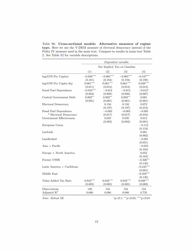
Table S6: Cross-sectional models: Alternative measures of regimetype. Here we use the V-DEM measure of electoral democracy instead of thePolity IV measure used in the main text. Compare to results in main text Table2. See Table S2 for variable descriptions.
Dependent variable:
Net Implicit Tax on Gasoline
(1) (2) (3) (4)
log(GNI Per Capita) −0.939∗∗∗ −0.965∗∗∗ −0.965∗∗∗ −0.547∗∗∗
(0.181) (0.194) (0.194) (0.198)log(GNI Per Capita Sq) 0.061∗∗∗ 0.061∗∗∗ 0.061∗∗∗ 0.038∗∗∗
(0.011) (0.012) (0.012) (0.012)Fossil Fuel Dependence −0.016∗∗∗ −0.013 −0.013 −0.013∗
(0.004) (0.008) (0.008) (0.007)Central Government Debt 0.002∗∗ 0.002∗∗ 0.002∗∗ 0.001
(0.001) (0.001) (0.001) (0.001)Electoral Democracy 0.156 0.156 0.072
(0.197) (0.197) (0.254)Fossil Fuel Dependence −0.003 −0.003 −0.005
* Electoral Democracy (0.017) (0.017) (0.016)Government Effectiveness 0.035 0.035 0.012
(0.082) (0.082) (0.081)European Union −0.112
(0.124)Latitude 0.001
(0.002)Landlocked −0.001
(0.051)Asia + Pacific −0.053
(0.104)Europe + North America 0.052
(0.163)Former USSR −0.326∗∗
(0.140)Latin America + Caribbean −0.245∗∗∗
(0.091)Middle East −0.359∗∗∗
(0.136)Value-Added Tax Rate 0.042∗∗∗ 0.042∗∗∗ 0.042∗∗∗ 0.038∗∗∗
(0.005) (0.005) (0.005) (0.008)
Observations 139 134 134 134Adjusted R2 0.660 0.686 0.686 0.735
Note: Robust SE ∗p<0.1; ∗∗p<0.05; ∗∗∗p<0.01
12
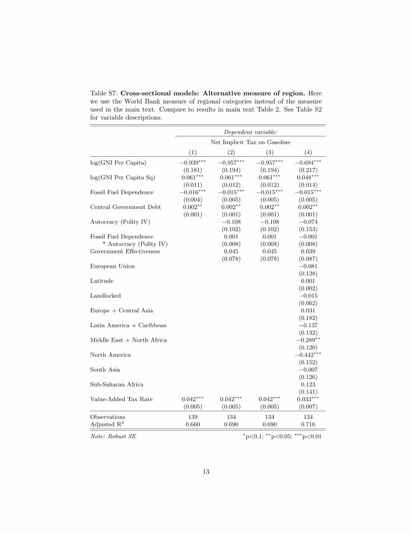
Table S7: Cross-sectional models: Alternative measure of region. Herewe use the World Bank measure of regional categories instead of the measureused in the main text. Compare to results in main text Table 2. See Table S2for variable descriptions.
Dependent variable:
Net Implicit Tax on Gasoline
(1) (2) (3) (4)
log(GNI Per Capita) −0.939∗∗∗ −0.957∗∗∗ −0.957∗∗∗ −0.694∗∗∗
(0.181) (0.194) (0.194) (0.217)log(GNI Per Capita Sq) 0.061∗∗∗ 0.061∗∗∗ 0.061∗∗∗ 0.048∗∗∗
(0.011) (0.012) (0.012) (0.014)Fossil Fuel Dependence −0.016∗∗∗ −0.015∗∗∗ −0.015∗∗∗ −0.015∗∗∗
(0.004) (0.005) (0.005) (0.005)Central Government Debt 0.002∗∗ 0.002∗∗ 0.002∗∗ 0.002∗∗
(0.001) (0.001) (0.001) (0.001)Autocracy (Polity IV) −0.108 −0.108 −0.074
(0.102) (0.102) (0.153)Fossil Fuel Dependence 0.001 0.001 −0.001
* Autocracy (Polity IV) (0.008) (0.008) (0.008)Government Effectiveness 0.045 0.045 0.039
(0.078) (0.078) (0.087)European Union −0.081
(0.128)Latitude 0.001
(0.002)Landlocked −0.015
(0.062)Europe + Central Asia 0.031
(0.182)Latin America + Caribbean −0.137
(0.132)Middle East + North Africa −0.289∗∗
(0.120)North America −0.442∗∗∗
(0.152)South Asia −0.007
(0.126)Sub-Saharan Africa 0.123
(0.141)Value-Added Tax Rate 0.042∗∗∗ 0.042∗∗∗ 0.042∗∗∗ 0.033∗∗∗
(0.005) (0.005) (0.005) (0.007)
Observations 139 134 134 134Adjusted R2 0.660 0.690 0.690 0.716
Note: Robust SE ∗p<0.1; ∗∗p<0.05; ∗∗∗p<0.01
13

Table S8: Cross-sectional models: National oil companies. Here we addmeasures to control for the presence of national oil companies. Compare toresults in main text Table 2. See Table S2 for variable descriptions.
Dependent variable:
Net Implicit Tax on Gasoline
(1) (2) (3)
log(GNI Per Capita) −0.879∗∗∗ −0.843∗∗∗ −0.879∗∗∗
(0.201) (0.173) (0.197)log(GNI Per Capita Sq) 0.055∗∗∗ 0.054∗∗∗ 0.056∗∗∗
(0.013) (0.011) (0.013)Fossil Fuel Dependence −0.011∗∗ −0.009∗ −0.012∗∗
(0.005) (0.005) (0.005)Central Government Debt 0.002∗∗ 0.002∗∗ 0.002∗∗
(0.001) (0.001) (0.001)Autocracy (Polity IV) −0.057 −0.024 −0.060
(0.095) (0.085) (0.100)Fossil Fuel Dependence * Autocracy −0.001 −0.003 −0.001
(0.008) (0.007) (0.008)Government Effectiveness 0.067 0.053 0.052
(0.078) (0.069) (0.077)National Oil Company (Mahdavi) −0.108∗
(0.059)Influential National Oil Company (Mahdavi) −0.252∗∗∗
(0.088)National Oil Company (Cheon et al.) −0.108
(0.066)Value-Added Tax Rate 0.041∗∗∗ 0.039∗∗∗ 0.041∗∗∗
(0.005) (0.005) (0.005)
Observations 132 132 134Adjusted R2 0.700 0.720 0.695
Note: Robust SE ∗p<0.1; ∗∗p<0.05; ∗∗∗p<0.01
14

Table S9: Cross-sectional models: Motorization rate. Here we add ameasure to control for the number of cars per capita, which plausibly representsthe size of the constituency benefiting directly from fuel subsidies. Compare toresults in main text Table 2. See Table S2 for variable descriptions.
Dependent variable:
Net Implicit Tax on Gasoline
(1) (2) (3) (4)
log(GNI Per Capita) −1.046∗∗∗ −1.064∗∗∗ −1.064∗∗∗ −0.741∗∗∗
(0.204) (0.218) (0.218) (0.248)log(GNI Per Capita Sq) 0.071∗∗∗ 0.070∗∗∗ 0.070∗∗∗ 0.054∗∗∗
(0.013) (0.015) (0.015) (0.017)Fossil Fuel Dependence −0.026∗∗∗ −0.022∗∗∗ −0.022∗∗∗ −0.023∗∗∗
(0.005) (0.007) (0.007) (0.006)Central Government Debt 0.001∗ 0.001 0.001 0.001
(0.001) (0.001) (0.001) (0.001)Autocracy (Polity IV) −0.105 −0.105 −0.072
(0.093) (0.093) (0.116)Fossil Fuel Dependence * Autocracy −0.001 −0.001 0.001
(0.008) (0.008) (0.007)Government Effectiveness 0.057 0.057 0.013
(0.082) (0.082) (0.093)Motorization Rate −0.315 −0.372 −0.372 −0.597
(0.292) (0.311) (0.311) (0.417)European Union −0.068
(0.126)Latitude 0.001
(0.002)Landlocked −0.006
(0.062)Asia + Pacific −0.054
(0.108)Europe + North America 0.089
(0.202)Former USSR −0.199
(0.186)Latin America + Caribbean −0.223∗∗
(0.100)Middle East −0.266∗∗
(0.129)Value-Added Tax Rate 0.042∗∗∗ 0.041∗∗∗ 0.041∗∗∗ 0.037∗∗∗
(0.005) (0.005) (0.005) (0.007)
Observations 117 113 113 113Adjusted R2 0.762 0.769 0.769 0.790
Note: Robust SE ∗p<0.1; ∗∗p<0.05; ∗∗∗p<0.01
15

2.2 Instrumental Variables models
Table S10: Instrumental Variables models: Alternative instrument.Here we use the spatial distribution of oil-yielding sedimentary basins, followingCassidy 2018, as an instrument for fossil fuel dependence instead of the oilendowment per capita instrument. Compare to results in main text Table 3.See Table S2 for variable descriptions and Table S11 for first-stage results.
Dependent variable:
Net Implicit Tax on Gasoline
(1) (2) (3)
log(GNI Per Capita)) −0.316 −0.358 −0.971∗∗∗
(0.392) (1.074) (0.362)log(GNI Per Capita Sq) 0.030 0.096 0.084∗∗
(0.021) (0.094) (0.040)Fossil Fuel Dependence −0.060∗∗ −0.183 −0.082
(0.025) (0.291) (0.094)Central Government Debt −0.0001 −0.007 −0.001
(0.002) (0.016) (0.004)Autocracy (Polity IV) −0.677 −0.259
(1.128) (0.364)Fossil Fuel Dependence * Autocracy 0.059 0.023
(0.116) (0.045)Government Effectiveness −1.550 −0.524
(2.780) (0.812)log(Land Area PC) 0.045 0.077 0.072
(0.055) (0.192) (0.113)log(Coastline PC) 0.008 0.052 0.010
(0.016) (0.107) (0.031)log(Mountainous Area PC) 0.007 0.033 −0.001
(0.015) (0.067) (0.018)log(Good Soil PC) −0.053∗ −0.144 −0.073
(0.030) (0.230) (0.082)log(Tropical Area PC) 0.016 0.051 0.022
(0.016) (0.074) (0.027)Europe/Northern America/Oceania −0.250 −1.128
(0.243) (2.059)Asia −0.223 −0.497
(0.171) (0.869)Latin America/Caribbean −0.364∗∗ −1.324
(0.183) (2.060)Value-Added Tax Rate 0.033∗∗∗ 0.064 0.044∗∗∗
(0.009) (0.047) (0.011)
Observations 135 131 131Adjusted R2 0.357 −2.920 0.040
Note: Robust SE ∗p<0.1; ∗∗p<0.05; ∗∗∗p<0.01
16
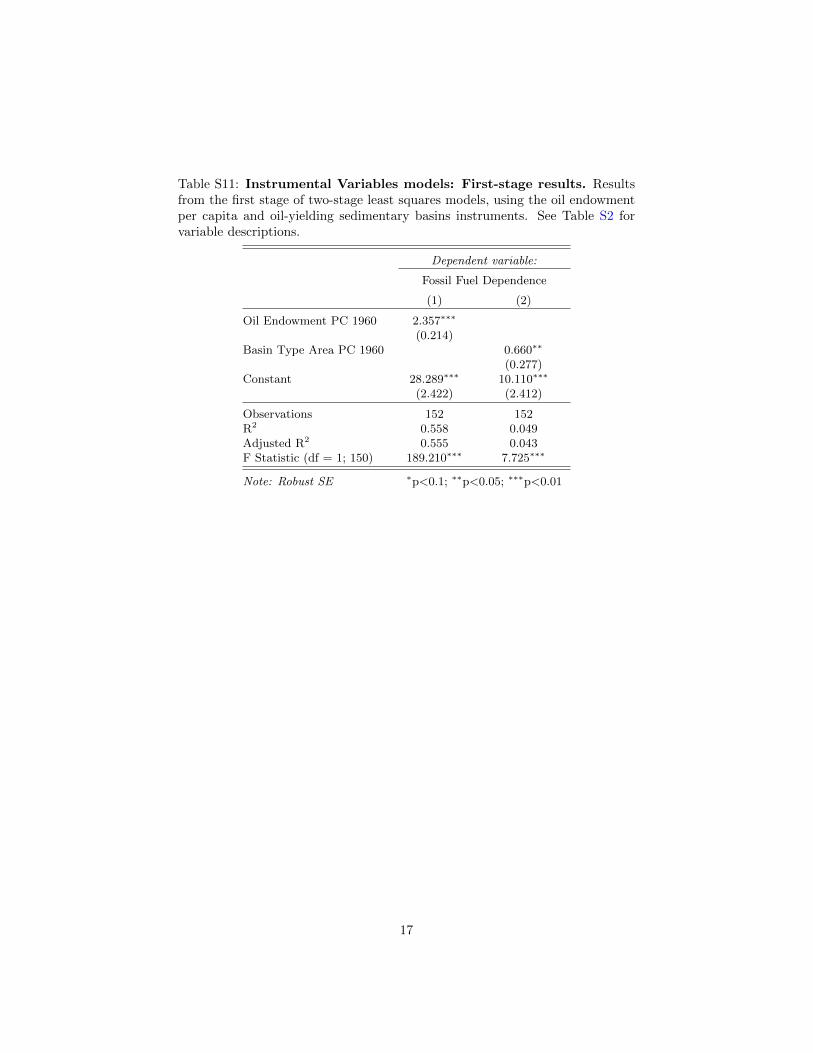
Table S11: Instrumental Variables models: First-stage results. Resultsfrom the first stage of two-stage least squares models, using the oil endowmentper capita and oil-yielding sedimentary basins instruments. See Table S2 forvariable descriptions.
Dependent variable:
Fossil Fuel Dependence
(1) (2)
Oil Endowment PC 1960 2.357∗∗∗
(0.214)Basin Type Area PC 1960 0.660∗∗
(0.277)Constant 28.289∗∗∗ 10.110∗∗∗
(2.422) (2.412)
Observations 152 152R2 0.558 0.049Adjusted R2 0.555 0.043F Statistic (df = 1; 150) 189.210∗∗∗ 7.725∗∗∗
Note: Robust SE ∗p<0.1; ∗∗p<0.05; ∗∗∗p<0.01
17

2.3 Cross-Sectional Time Series models
A Hausman test comparing the pooled OLS model to a country-year fixed ef-fects model gives an F statistic of 34.9 (p-value < 0.0001), which suggests thefixed effects model may be a better choice over the pooled model. (A secondHausman test gives a χ2 of 99.97 (p-value < 0.0001), indicating that a randomeffects model should be rejected in favor of a fixed effects model.) In a pooledmodel, GNI per capita, GNI per capita sq, Fossil Fuel Dependence, and CentralGovernment Debt have the same relationships to Net Implicit Tax on Gasolineas they do in the cross-section results in the main text (Tables 1-3). We alsofind that Autocracy is statistically associated with Net Implicit Tax on Gasolinein the direction hypothesized by prior studies, while Government Effectivenessis not. The Fossil Fuel Dependence*Autocracy interaction term remains notstatistically significant, implying that fossil fuel dependence has similar effectsin democracies and autocracies. Note that, as discussed in the main text, oncecountry and year fixed effects are added to the model, most of the variables losestatistical significance at the p = 0.05 level (although Autocracy remains signif-icant at the p = 0.10 level). The exceptions are Fossil Fuel Dependence, VAT,and Central Government Debt, which remain significant in both specifications.
Table S12: Cross-sectional Time-series: with and without fixed effects.Compare to Table 4 in the main text. See Table S2 for variable descriptions.
Dependent variable:
Net Implicit Tax on Gasoline
(1) (2)
log(GNI Per Capita) −0.843∗∗∗ −0.020(0.058) (0.097)
log(GNI Per Capita Sq) 0.055∗∗∗ 0.004(0.004) (0.006)
Oil and Gas Income Dependence −0.014∗∗∗ −0.006∗∗∗
(0.001) (0.002)Central Government Debt 0.001∗∗∗ 0.001∗∗∗
(0.0003) (0.0003)Autocracy (Polity IV) −0.149∗∗∗ 0.096∗
(0.040) (0.054)Oil and Gas Income Dependence * Autocracy −0.0001 −0.005
(0.003) (0.003)Government Effectiveness 0.033 0.026
(0.021) (0.031)Value-Added Tax Rate 0.040∗∗∗ 0.018∗∗∗
(0.002) (0.004)Constant 3.000∗∗∗ 0.147
(0.237) (0.400)
Observations 1,522 1,522Country and Year FE N YR2 0.645 0.938Adjusted R2 0.643 0.931
Note: Robust SE ∗p<0.1; ∗∗p<0.05; ∗∗∗p<0.01
18

Table S13: Cross-sectional time-series models: Alternative measuresof regime type. Here we use the Boix-Miller-Rosato measure of democracyinstead of the Polity IV measure used in the main text. Compare to results inmain text Table 4. See Table S2 for variable descriptions.
Dependent variable:
Net Implicit Tax on Gasoline
(1) (2)
log(GNI Per Capita) −0.848∗∗∗ −0.033(0.061) (0.096)
log(GNI Per Capita Sq) 0.055∗∗∗ 0.005(0.004) (0.006)
Fossil Fuel Dependence −0.014∗∗∗ −0.010∗∗∗
(0.002) (0.002)Central Government Debt 0.001∗∗∗ 0.001∗∗∗
(0.0003) (0.0003)Democracy 0.065∗∗∗ 0.009
(0.023) (0.033)Fossil Fuel Dependence * Democracy −0.002 0.008∗∗
(0.003) (0.004)Government Effectiveness 0.035∗ 0.045
(0.021) (0.030)Value-Added Tax Rate 0.042∗∗∗ 0.017∗∗∗
(0.002) (0.004)Constant 2.971∗∗∗ 0.247
(0.246) (0.393)
Observations 1,547 1,547Country and Year FE N YR2 0.636 0.937Adjusted R2 0.634 0.930
Note: Robust SE ∗p<0.1; ∗∗p<0.05; ∗∗∗p<0.01
19

Table S14: Cross-sectional time-series models: Alternative measures ofregime type. Here we use the V-Dem measure of electoral democracy insteadof the Polity IV measure used in the main text. Compare to results in maintext Table 4. See Table S2 for variable descriptions.
Dependent variable:
Net Implicit Tax on Gasoline
(1) (2)
log(GNI Per Capita) −0.850∗∗∗ −0.059(0.059) (0.099)
log(GNI Per Capita Sq) 0.055∗∗∗ 0.006(0.004) (0.006)
Fossil Fuel Dependence −0.014∗∗∗ −0.011∗∗∗
(0.003) (0.003)Central Government Debt 0.001∗∗∗ 0.001∗∗∗
(0.0003) (0.0003)Electoral Democracy 0.167∗∗∗ 0.052
(0.060) (0.078)Fossil Fuel Dependence * Electoral Democracy −0.002 0.008
(0.005) (0.007)Government Effectiveness 0.023 0.045
(0.021) (0.030)Value-Added Tax Rate 0.041∗∗∗ 0.017∗∗∗
(0.002) (0.004)Constant 2.960∗∗∗ 0.346
(0.240) (0.400)
Observations 1,537 1,537Country and Year FE N YR2 0.640 0.937Adjusted R2 0.638 0.930
Note: Robust SE ∗p<0.1; ∗∗p<0.05; ∗∗∗p<0.01
20

Table S15: Cross-sectional time-series models: Motorization rate. Herewe add a measure to control for the number of cars per capita, which plausiblyrepresents the size of the constituency benefiting directly from fuel subsidies.Compare to results in main text Table 2. See Table S2 for variable descriptions.
Dependent variable:
Net Implicit Tax on Gasoline
(1) (2)
log(GNI Per Capita) −0.967∗∗∗ −0.233∗
(0.073) (0.137)log(GNI Per Capita Sq) 0.062∗∗∗ 0.015∗
(0.005) (0.008)Fossil Fuel Dependence −0.020∗∗∗ −0.001
(0.002) (0.002)Central Government Debt 0.001∗∗ 0.001∗∗∗
(0.0003) (0.0004)Autocracy (Polity IV) −0.195∗∗∗ 0.147∗∗
(0.044) (0.059)Fossil Fuel Dependence * Autocracy 0.004 −0.002
(0.003) (0.003)Government Effectiveness 0.086∗∗∗ −0.007
(0.026) (0.037)Motorization Rate −0.222∗∗ 0.450∗
(0.103) (0.238)Value-Added Tax Rate 0.043∗∗∗ 0.014∗∗∗
(0.002) (0.004)Constant 3.548∗∗∗ 0.988∗
(0.285) (0.550)
Observations 1,093 1,093Country and Year FE N YR2 0.738 0.961Adjusted R2 0.736 0.956
Note: Robust SE ∗p<0.1; ∗∗p<0.05; ∗∗∗p<0.01
21
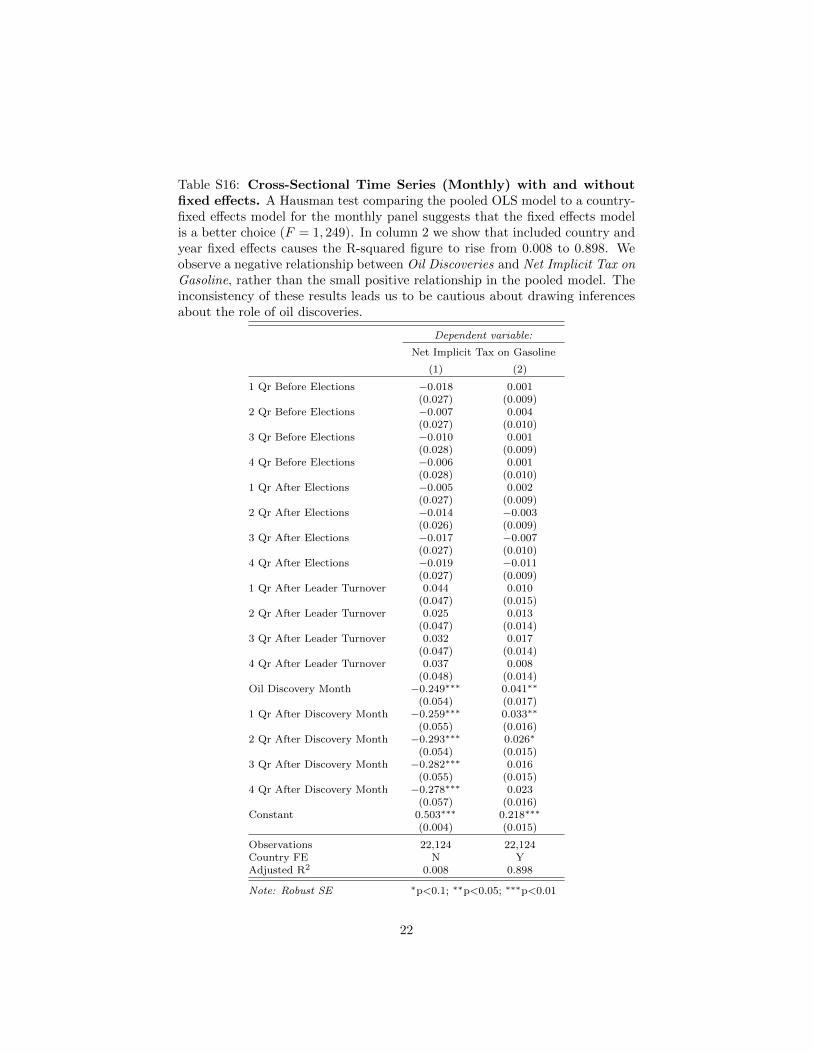
Table S16: Cross-Sectional Time Series (Monthly) with and withoutfixed effects. A Hausman test comparing the pooled OLS model to a country-fixed effects model for the monthly panel suggests that the fixed effects modelis a better choice (F = 1, 249). In column 2 we show that included country andyear fixed effects causes the R-squared figure to rise from 0.008 to 0.898. Weobserve a negative relationship between Oil Discoveries and Net Implicit Tax onGasoline, rather than the small positive relationship in the pooled model. Theinconsistency of these results leads us to be cautious about drawing inferencesabout the role of oil discoveries.
Dependent variable:
Net Implicit Tax on Gasoline
(1) (2)
1 Qr Before Elections −0.018 0.001(0.027) (0.009)
2 Qr Before Elections −0.007 0.004(0.027) (0.010)
3 Qr Before Elections −0.010 0.001(0.028) (0.009)
4 Qr Before Elections −0.006 0.001(0.028) (0.010)
1 Qr After Elections −0.005 0.002(0.027) (0.009)
2 Qr After Elections −0.014 −0.003(0.026) (0.009)
3 Qr After Elections −0.017 −0.007(0.027) (0.010)
4 Qr After Elections −0.019 −0.011(0.027) (0.009)
1 Qr After Leader Turnover 0.044 0.010(0.047) (0.015)
2 Qr After Leader Turnover 0.025 0.013(0.047) (0.014)
3 Qr After Leader Turnover 0.032 0.017(0.047) (0.014)
4 Qr After Leader Turnover 0.037 0.008(0.048) (0.014)
Oil Discovery Month −0.249∗∗∗ 0.041∗∗
(0.054) (0.017)1 Qr After Discovery Month −0.259∗∗∗ 0.033∗∗
(0.055) (0.016)2 Qr After Discovery Month −0.293∗∗∗ 0.026∗
(0.054) (0.015)3 Qr After Discovery Month −0.282∗∗∗ 0.016
(0.055) (0.015)4 Qr After Discovery Month −0.278∗∗∗ 0.023
(0.057) (0.016)Constant 0.503∗∗∗ 0.218∗∗∗
(0.004) (0.015)
Observations 22,124 22,124Country FE N YAdjusted R2 0.008 0.898
Note: Robust SE ∗p<0.1; ∗∗p<0.05; ∗∗∗p<0.01
22

3 Supplementary Tables: Diesel models
We additionally run all specifications in the main text for models with taxeson diesel fuel instead of gasoline. The same core patterns hold for diesel: aconsistent statistical relationship between fuel taxes and income, and betweenfuel taxes and fossil fuel dependence; the lack of a consistent relationship withpolitical factors; and the importance of unobserved, country-specific factors inthe annual panel. Note that we do not run monthly panels here given the lackof infra-annual data on diesel prices.
3.1 Cross-Sectional models
Table S17: Diesel analysis: cross-sectional base specification. Compareto results in main text Table 1. See Table S2 for variable descriptions.
Dependent variable:
Net Implicit Tax on Diesel
(1) (2) (3) (4)
log(GNI Per Capita) −0.899∗∗∗ −0.820∗∗∗ −0.780∗∗∗ −0.664∗∗∗
(0.163) (0.150) (0.145) (0.146)log(GNI Per Capita Sq) 0.057∗∗∗ 0.053∗∗∗ 0.050∗∗∗ 0.044∗∗∗
(0.010) (0.009) (0.009) (0.009)Fossil Fuel Dependence −0.015∗∗∗
(0.003)log(Oil and Gas Exports PC) −0.019∗∗∗
(0.004)Fossil Fuel Export Dependence −0.006∗∗∗
(0.001)Central Government Debt 0.001∗∗ 0.001 0.001 0.0005
(0.001) (0.001) (0.001) (0.001)Value-Added Tax Rate 0.042∗∗∗ 0.034∗∗∗ 0.035∗∗∗ 0.030∗∗∗
(0.004) (0.004) (0.004) (0.004)Constant 3.101∗∗∗ 2.953∗∗∗ 2.692∗∗∗ 2.433∗∗∗
(0.676) (0.606) (0.597) (0.594)
Observations 138 137 137 135R2 0.587 0.666 0.656 0.722Adjusted R2 0.575 0.653 0.643 0.711
Note: Robust SE ∗p<0.1; ∗∗p<0.05; ∗∗∗p<0.01
23

Table S18: Diesel analysis: cross-sectional full specification. Compareto results in main text Table 2. See Table S2 for variable descriptions.
Dependent variable:
Net Implicit Tax on Diesel
(1) (2) (3) (4)
log(GNI Per Capita) −0.820∗∗∗ −0.904∗∗∗ −0.904∗∗∗ −0.420∗∗∗
(0.150) (0.158) (0.158) (0.159)log(GNI Per Capita Sq) 0.053∗∗∗ 0.059∗∗∗ 0.059∗∗∗ 0.031∗∗∗
(0.009) (0.010) (0.010) (0.010)Fossil Fuel Dependence −0.015∗∗∗ −0.016∗∗∗ −0.016∗∗∗ −0.016∗∗∗
(0.003) (0.004) (0.004) (0.004)Central Government Debt 0.001 0.001 0.001 0.0005
(0.001) (0.001) (0.001) (0.001)Autocracy (Polity IV) −0.147∗ −0.147∗ −0.115
(0.079) (0.079) (0.081)Fossil Fuel Dependence * Autocracy −0.002 −0.002 0.001
(0.006) (0.006) (0.005)Government Effectiveness −0.025 −0.025 −0.027
(0.067) (0.067) (0.066)European Union −0.033
(0.099)Latitude 0.002
(0.001)Landlocked 0.070∗
(0.041)Asia + Pacific −0.171∗∗
(0.073)Europe + North America −0.002
(0.129)Former USSR −0.279∗∗
(0.110)Latin America + Caribbean −0.243∗∗∗
(0.065)Middle East −0.336∗∗∗
(0.112)Value-Added Tax Rate 0.034∗∗∗ 0.034∗∗∗ 0.034∗∗∗ 0.026∗∗∗
(0.004) (0.004) (0.004) (0.006)Constant 2.953∗∗∗ 3.226∗∗∗ 3.226∗∗∗ 1.433∗∗
(0.606) (0.620) (0.620) (0.619)
Observations 137 132 132 132R2 0.666 0.725 0.725 0.793Adjusted R2 0.653 0.707 0.707 0.765
Note: Robust SE ∗p<0.1; ∗∗p<0.05; ∗∗∗p<0.01
24

3.2 Instrumental Variables models
Table S19: Diesel analysis: instrumental variable specification. Fossilfuel dependence is instrumented using the oil endowment per capita measurefrom 1960. Compare to results in main text Table 3.
Dependent variable:
Net Implicit Tax on Diesel
(1) (2) (3) (4)
log(GNI Per Capita) −0.795∗∗∗ −0.962∗∗∗ −0.962∗∗∗ −0.411∗∗
(0.166) (0.164) (0.164) (0.181)log(GNI Per Capita Sq) 0.052∗∗∗ 0.066∗∗∗ 0.066∗∗∗ 0.035∗∗∗
(0.010) (0.011) (0.011) (0.011)Fossil Fuel Dependence −0.025∗∗∗ −0.025∗∗∗ −0.025∗∗∗ −0.026∗∗∗
(0.004) (0.005) (0.005) (0.005)Central Government Debt −0.00004 0.0002 0.0002 0.00001
(0.001) (0.001) (0.001) (0.001)Autocracy (Polity IV) −0.178 −0.178 −0.148
(0.116) (0.116) (0.111)Fossil Fuel Dependence * Autocracy 0.003 0.003 0.006
(0.007) (0.007) (0.007)Government Effectiveness −0.114∗ −0.114∗ −0.126∗
(0.066) (0.066) (0.069)European Union −0.076
(0.088)Latitude 0.002
(0.001)Landlocked 0.052
(0.052)Asia + Pacific −0.213∗∗∗
(0.080)Europe + North America −0.099
(0.132)Former USSR −0.367∗∗∗
(0.131)Latin America + Caribbean −0.323∗∗∗
(0.082)Middle East −0.373∗∗∗
(0.103)Value-Added Tax Rate 0.029∗∗∗ 0.032∗∗∗ 0.032∗∗∗ 0.027∗∗∗
(0.004) (0.004) (0.004) (0.005)Constant 2.974∗∗∗ 3.307∗∗∗ 3.307∗∗∗ 1.157
(0.695) (0.656) (0.656) (0.750)
Observations 135 130 130 130R2 0.627 0.705 0.705 0.771Adjusted R2 0.612 0.686 0.686 0.739
Note: Robust SE ∗p<0.1; ∗∗p<0.05; ∗∗∗p<0.01
25

3.3 Cross-Sectional Time Series models
Table S20: Diesel analysis: cross-sectional time-series specification.Compare to results in main text Table 4. See Table S2 for variable descrip-tions.
Dependent variable:
Net Implicit Tax on Diesel
(1) (2)
log(GNI Per Capita) −0.796∗∗∗ −0.208(0.069) (0.132)
log(GNI Per Capita Sq) 0.052∗∗∗ 0.012(0.004) (0.008)
Oil and Gas Income Dependence −0.015∗∗∗ −0.005∗
(0.002) (0.003)Autocracy (Polity IV) −0.159∗∗∗ 0.065
(0.041) (0.067)Government Effectiveness −0.004 0.058
(0.029) (0.045)Central Government Debt 0.0001 0.0004
(0.0003) (0.0004)Oil and Gas Income Dependence * Autocracy −0.001 0.0004
(0.003) (0.005)Value-Added Tax Rate 0.035∗∗∗ 0.011∗∗
(0.002) (0.006)Constant 2.807∗∗∗ 1.247∗∗
(0.273) (0.549)
Observations 734 734Country and Year FE N YR2 0.657 0.930Adjusted R2 0.653 0.913
Note: Robust SE ∗p<0.1; ∗∗p<0.05; ∗∗∗p<0.01
26

4 Supplementary Figures
0.0
0.5
1.0
1.5
5 6 7 8 9 10 11
Income per capita (logged)
Pre
dict
ed N
et im
plic
it ta
x on
gas
olin
e (
cons
tant
201
5 U
SD
per
lite
r)
Figure S1: Income per capita and predicted fuel taxes by country.Marginal effects of logged income per capita and logged income per capitasquared on fuel taxes, based on results from Table 1, column 1. Predictedvalues for fuel taxes are plotted on the y-axis. Distribution of logged incomeper capita values plotted as a rug above the x-axis.
27

1st
2nd
3rd
4th
−1.00
−0.50
0.00
0.50
1.00
1.50
$2.00
2003 2004 2005 2006 2007 2008 2009 2010 2011 2012 2013 2014 2015 2016
Year
Net
impl
icit
tax
on g
asol
ine
(co
nsta
nt 2
015
US
D p
er li
ter)
Figure S2: Net taxes and subsidies by income group over time. Incomegroup averages are computed monthly using unweighted country taxes and sub-sidies. This figure excludes oil-exporting countries. Color-coding is as follows,from top to bottom as of 2015. Black: first income quartile; blue: second incomequartile; green: fourth income quartile, orange: third income quartile.
28
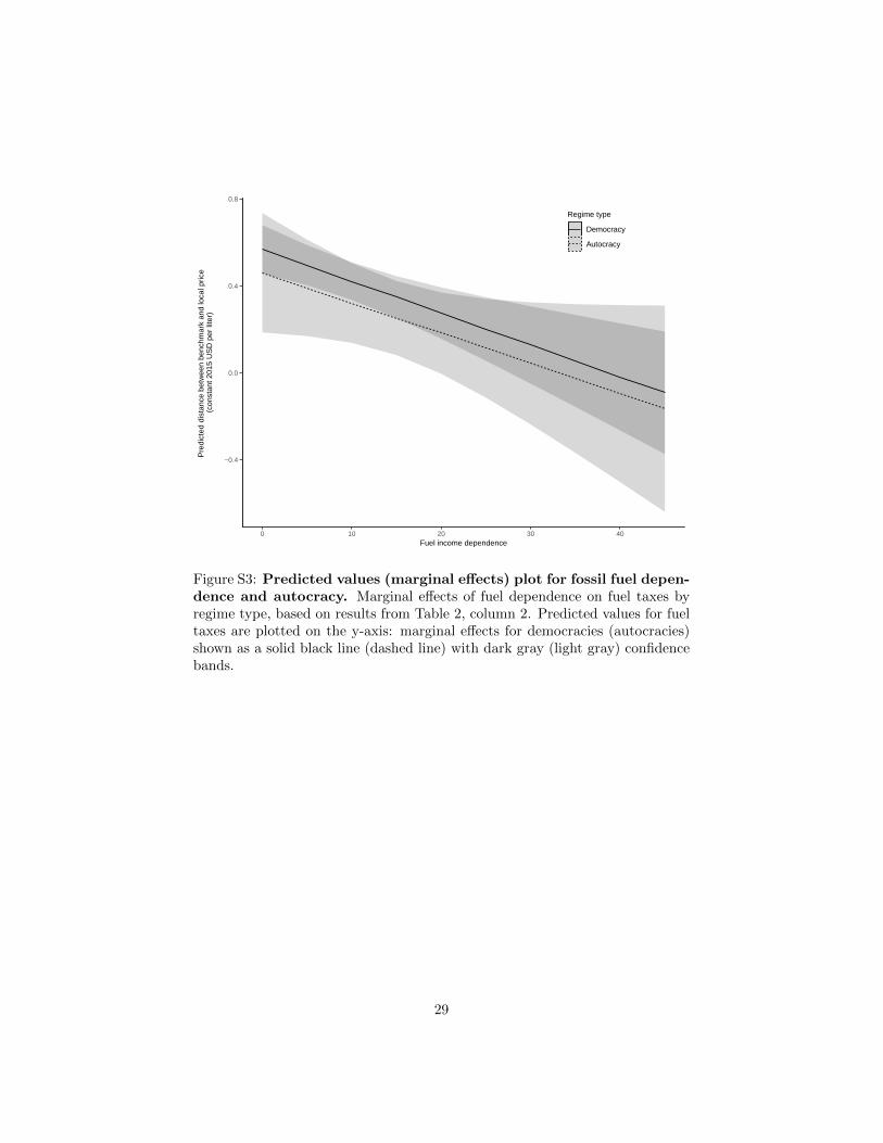
−0.4
0.0
0.4
0.8
0 10 20 30 40Fuel income dependence
Pre
dict
ed d
ista
nce
betw
een
benc
hmar
k an
d lo
cal p
rice
(co
nsta
nt 2
015
US
D p
er li
ter)
Regime type
Democracy
Autocracy
Figure S3: Predicted values (marginal effects) plot for fossil fuel depen-dence and autocracy. Marginal effects of fuel dependence on fuel taxes byregime type, based on results from Table 2, column 2. Predicted values for fueltaxes are plotted on the y-axis: marginal effects for democracies (autocracies)shown as a solid black line (dashed line) with dark gray (light gray) confidencebands.
29

Figure S4 illustrates the importance of Fossil Fuel Dependence: it is similarto Figure 5 in the main text but highlights countries above the 30% Fossil FuelExport Dependence threshold. Of the 27 oil exporters, 20 had net subsidies ineither 2003, 2015, or both. Sixteen of them also fall below the 45 degree line,indicating that their taxes fell (or subsidies grew) during this period.
Angola
United Arab Emirates
Argentina
Armenia
Australia
Austria
Azerbaijan
Burundi
Belgium
Benin
Burkina Faso
Bangladesh
Bulgaria
Bahrain
Bosnia and Herzegovina
Belize
Bolivia
Brazil
Botswana
Central African Republic
Canada
Switzerland
Chile
China
Cote d'Ivoire
Cameroon
Congo, Dem. Rep.
Congo, Rep.
Colombia
Costa RicaCzech Republic
GermanyDenmark
Dominican Republic
Algeria
EcuadorEgypt, Arab Rep.
Spain
Estonia
Finland
France
Gabon
United Kingdom
Gambia, The Guinea−Bissau
Equatorial Guinea
Greece
Guatemala
Guyana
Croatia
Hungary
Indonesia
India
Ireland
Iran, Islamic Rep.
Iraq
Israel Italy
Jordan
Japan
Kenya
Kyrgyz Republic
Cambodia
Korea, Rep.
Kuwait
Lebanon
Libya
Sri Lanka
Lithuania Luxembourg
Latvia
Morocco
Moldova
Madagascar
Mexico
Mali
Mongolia
Mozambique
Mauritania Mauritius
Malawi
Malaysia
Namibia
Niger
Nigeria
Nicaragua
Netherlands
Norway
Nepal
New Zealand
Oman
Panama Peru
Philippines
Portugal
Paraguay
Qatar
Romania
Russian Federation
Rwanda
Saudi Arabia
Senegal
Singapore
Sierra Leone
Serbia
Suriname
SloveniaSweden
Swaziland
Syrian Arab RepublicChad
Togo
Thailand
Tajikistan
Trinidad and Tobago
Turkey
Taiwan
Tanzania
Uganda
Ukraine
Uruguay
United States
Venezuela
Vietnam
Yemen, Rep.
South Africa
Zambia
−0.50
−0.25
0.00
0.25
0.50
0.75
1.00
1.25
−0.25 0.00 0.25 0.50 0.75 1.00 1.25
Net implicit tax on gasoline in 1st half 2003 (constant 2015 USD per litre)
Net
impl
icit
tax
on g
asol
ine
in 1
st h
alf 2
015
(con
stan
t 201
5 U
SD
per
litr
e)
Gasoline consumption (thou. bbls per day)
a
a1000
5000
Figure S4: Net VAT-adjusted implicit taxes in 2003 versus 2015 forfuel dependent countries. The average level of taxes or subsidies per literfor countries in the first six months of 2003 compared to the first six monthsof 2015, with highlighted labels for the top 30 most fuel dependent countries.Countries with higher taxes (or lower subsidies) in 2015 than in 2003 are coloredin blue; those with lower taxes (or higher subsidies) are colored in dark orange.See notes in Figure 5 for further details.
30
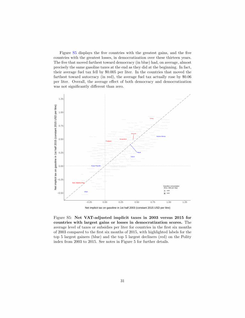
Figure S5 displays the five countries with the greatest gains, and the fivecountries with the greatest losses, in democratization over these thirteen years.The five that moved farthest toward democracy (in blue) had, on average, almostprecisely the same gasoline taxes at the end as they did at the beginning. In fact,their average fuel tax fell by $0.005 per liter. In the countries that moved thefarthest toward autocracy (in red), the average fuel tax actually rose by $0.06per liter. Overall, the average effect of both democracy and democratizationwas not significantly different than zero.
Angola
United Arab Emirates
Argentina
Armenia
Australia
Austria
Azerbaijan
Burundi
Belgium
Benin
Burkina Faso
Bangladesh
Bulgaria
Bahrain
Bosnia and Herzegovina
Belize
Bolivia
Brazil
Botswana
Central African Republic
Canada
Switzerland
Chile
ChinaCote d'IvoireCameroon
Congo, Dem. Rep.
Congo, Rep.
Colombia
Costa Rica
Czech Republic
GermanyDenmark
Dominican Republic
Algeria
EcuadorEgypt, Arab Rep.
Spain
Estonia
Finland
France
Gabon
United Kingdom
Gambia, The Guinea−Bissau
Equatorial Guinea
Greece
Guatemala
Guyana
Croatia
Hungary
Indonesia
India
Ireland
Iran, Islamic Rep.
Iraq
Israel Italy
Jordan
Japan
Kenya
Kyrgyz Republic
Cambodia
Korea, Rep.
Kuwait
Lebanon
Libya
Sri Lanka
LithuaniaLuxembourg
Latvia
Morocco
Moldova
Madagascar
Mexico
Mali
Mongolia
Mozambique
Mauritania Mauritius
Malawi
Malaysia
Namibia
Niger
Nigeria
Nicaragua
Netherlands
Norway
Nepal
New Zealand
Oman
Panama
Peru
Philippines
Portugal
Paraguay
Qatar
Romania
Russian Federation
Rwanda
Saudi Arabia
Senegal
Singapore
Sierra Leone
SerbiaSuriname
SloveniaSweden
Swaziland
Syrian Arab Republic Chad
Togo
Thailand
Tajikistan
Trinidad and Tobago
Turkey
Taiwan
Tanzania
Uganda
Ukraine
Uruguay
United States
Venezuela
Vietnam
Yemen, Rep.
South Africa
Zambia
−0.50
−0.25
0.00
0.25
0.50
0.75
1.00
1.25
−0.25 0.00 0.25 0.50 0.75 1.00 1.25
Net implicit tax on gasoline in 1st half 2003 (constant 2015 USD per litre)
Net
impl
icit
tax
on g
asol
ine
in 1
st h
alf 2
015
(con
stan
t 201
5 U
SD
per
litr
e)
Gasoline consumption (thou. bbls per day)
a
a1000
5000
Figure S5: Net VAT-adjusted implicit taxes in 2003 versus 2015 forcountries with largest gains or losses in democratization scores. Theaverage level of taxes or subsidies per liter for countries in the first six monthsof 2003 compared to the first six months of 2015, with highlighted labels for thetop 5 largest gainers (blue) and the top 5 largest decliners (red) on the Polityindex from 2003 to 2015. See notes in Figure 5 for further details.
31

References
Africa News (2018). “Burkina faso: Protest against fuel price increase”,11/30/2018.
Al-Jazeera (2014). “Yemen protests erupt after fuel price doubles”, 07/30/2014.
Arezki, R., Ramey, V. A., and Sheng, L. (2017). News shocks in open economies:Evidence from giant oil discoveries. The Quarterly Journal of Economics,132(1):103–155.
Asia Times (2007). “Fuel price policy explodes in myanmar”, 07/24/2007.
Boix, C., Miller, M., and Rosato, S. (2013). A complete data set of politicalregimes, 1800–2007. Comparative Political Studies, 46(12):1523–1554.
Cassidy, T. (2018). The long-run effects of oil wealth on development: Evidencefrom petroleum geology. The Economic Journal, 129(623):2745–2778.
Coppedge, M., Gerring, J., Lindberg, S. I., Teorell, J., Altman, D., Bernhard,M., Fish, M. S., Glynn, A., Hicken, A., Knutsen, C. H., et al. (2015). Varietiesof democracy. Codebook. Version.
EIA (2019a). Cushing ok wti spot price fob.
EIA (2019b). Spot price for conventional refined gasoline atthe new york cityport.
EIA (2019c). Spot price for ultra low sulfur carb diesel.
Goemans, H. E., Gleditsch, K. S., and Chiozza, G. (2009). Introducing archigos:A dataset of political leaders. Journal of Peace research, 46(2):269–283.
Hyde, S. D. and Marinov, N. (2015). Nelda 4.0: National elections across democ-racy and autocracy dataset codebook for version 4. Accessed on September,2:2016.
IMF (2019a). Central government debt database.
IMF (2019b). Value-added tax rates database.
Mahdavi, P. (2020). Power Grab: Political Survival Through Extractive ResourceNationalization. Cambridge: Cambridge University Press.
Marshall, M. G., Jaggers, K., and Gurr, T. R. (2011). Polity IV project: Politicalregime characteristics and transitions 1800-2010 dataset users manual. Centerfor Systemic Peace, 11.
Ortiz, I., Burke, S., Berrada, M., and Cortes, H. (2013). World protests 2006-2013. Initiative for Policy Dialogue and Friedrich-Ebert-Stiftung New YorkWorking Paper, (2013).
32

Ross, M. L. (2013). The oil curse: How petroleum wealth shapes the developmentof nations. Princeton University Press.
Ross, M. L., Hazlett, C., and Mahdavi, P. (2017). Global progress and back-sliding on gasoline taxes and subsidies. Nature Energy, 2(1):16201.
The Guardian (2019). “Brazil faces call for return to military dictatorship amidtruckers’ strike”, 05/30/2019.
The Jordan Times (2013a). “Activists protest against fuel price rise”,03/02/2013.
The Jordan Times (2013b). “Sudan defends crackdown as protests enter secondweek”, 09/30/2013.
The New York Times (2008). “Anti government rioting spreads in Cameroon”,12/07/2008.
The New York Times (2018). “Hundreds of thousands in France protest taxesby blocking roads”, 11/17/2018.
The New York Times (2019a). “Deal struck in Ecuador to cancel austeritypackage and end protests”, 10/13/2019.
The New York Times (2019b). “Iran abruptly raises fuel prices, and protestserupt”, 11/18/2019.
The Washington Post (2008). “Mexicans are outraged over a big hike in gasprices on jan 1”, 01/02/2017.
Tsui, K. K. (2011). More oil, less democracy: Evidence from worldwide crudeoil discoveries. The Economic Journal, 121(551):89–115.
World Bank (2019). World development indicators database.
33