Whole System Design Suite - research.qut.edu.au · and arbitrary spot, and the pipe fitter is then...

Technical Design Portfolio

Whole System Design Suite Taking a whole system approach to achieving

sustainable design outcomes

Unit 6 - Worked Example 1 Industrial Pumping Systems

July 2007

This Course was developed under a grant from the Australian Government Department of the Environment and Water Resources as

part of the 2005/06 Environmental Education Grants Program. (The views expressed herein are not necessarily the views of the

Commonwealth, and the Commonwealth does not accept the responsibility for any information or advice contained herein.)

TDP ESSP Technical Design Portfolio: Whole System Design Suite Worked Example 1 – Industrial Pumping Systems

Unit 6 Worked Example 1 – Industrial Pumping

Systems

Significance of Pumping Systems and Design Motors use 60 percent of the world’s electricity. Of this percentage, 20 percent is used for pumping.1 Industrial pumping systems account for nearly 20 percent of the world’s industrial electrical energy demand; this is no surprise, as most systems are running in continuous operations for 18 hours per day or more.

With such a large amount of energy devoted to moving liquid from one place to another (a lot of which is used to fight pipe friction and in many cases unnecessary changes in height and direction), improving the efficiency of industrial pumping systems can make major strides in the reduction of industrial energy consumption and hence greenhouse emissions. The benefits of improved pumping efficiency include reduced reliance on both the electricity grid and renewable energy supplies, and improved operational reliability. Furthermore, saving a single unit of pumping energy can actually save more than ten times that energy in fuel. Due to the inefficiencies of a mostly centralised electricity transmission system, 100 units of fuel input at the power station are required to achieve 9.5 units of energy output at the pumping system.2 But the reverse is also true: saving 9.5 units of energy output at the pump could save 100 units of energy at the power station.3

Generally, smaller pumping systems tend to be more inefficient than large pumping systems. Small pumping systems typically make up only a small fraction of the total cost of an industrial operation and thus receive relatively little design attention. However, the significance of small pumping systems cannot be overlooked. There are many more small- and medium-sized enterprises than there are large enterprises. Thus it is likely that there are a lot more small pumping systems than large pumping systems, especially since small enterprises almost exclusively use small pumping systems and large enterprises use both small and large pumping systems. Large pumping systems, in the order of kilowatts and megawatts that are poorly designed and managed, can attract very high and unnecessary costs. Consequently, large pumping system design is typically quite disciplined, with more attention paid to factors such as minimum velocities, thermal expansion, pipe work and maintenance. Still, there are very few pumping systems that wouldn’t benefit from Whole System Design.

1 Hawken, P., Lovins, A.B. and Lovins, L.H. (1999) Natural Capitalism: Creating the Next Industrial Revolution, Earthscan, London p 115. 2 Ibid, p 121 3 Ibid, p 121

Prepared by The Natural Edge Project 2007 of 21


Worked example overview

The following worked example provides a worked mathematical example similar to a well known Whole System Design case study, ‘Pipes and Pumps’, which is briefly described in the below extract from Natural Capitalism:4

In 1997, leading American carpet maker, Interface Inc, was building a factory in Shanghai. One of its industrial processes required fourteen pumps. In optimizing the design, the top Western specialist firm sized those pumps to total ninety-five horsepower. But a fresh look by Interface/Holland's engineer Jan Schilham, applying methods learned from Singaporean efficiency expert Eng Lock Lee, cut the design's pumping power to only seven horsepower - a 92 percent or twelve-fold energy saving - while reducing its capital cost and improving its performance in every respect.

The new specifications required two changes in design. First, Schilham chose to deploy big pipes and small pumps instead of the original design's small pipes and big pumps. Friction falls as nearly the fifth power of pipe diameter, so making the pipes 50 percent fatter reduces their friction by 86 percent. The system then needs less pumping energy - and smaller pumps and motors to push against the friction. If the solution is this easy, why weren't the pipes originally specified to be big enough? Because of a small but important blind spot: traditional optimization compares the cost of the fatter pipe with only the value of the saved pumping energy. This comparison ignores the size, and hence the capital cost, of the equipment - pump, motor, motor-drive circuits, and electrical supply components - needed to combat the pipe friction. Schilham found he needn't calculate how quickly the savings could repay the extra up-front cost of the fatter pipe, because capital cost would fall more for the pumping and drive equipment than it would rise for the pipe, making the efficient system as a whole cheaper to construct.

Second, Schilham laid out the pipes first and then installed the equipment, in reverse to how pumping systems are conventionally installed. Normally, equipment is put in some convenient and arbitrary spot, and the pipe fitter is then instructed to connect point A to point B. The pipe often has to go through all sorts of twists and turns to hook up equipment that's too far apart, turned the wrong way, mounted at the wrong height, and separated by other devices installed in between. The extra bends and the extra length make friction in the system about three- to sixfold higher than it should be. The pipe fitters don't mind the extra work: They're paid by the hour, they mark up the pipe and fittings, and they won't have to pay the pumps' capital or operating costs.

By laying out the pipes before placing the equipment that the pipes connect, Schilham was able to make the pipes short and straight rather than long and crooked. That enabled him to exploit their lower friction by making the pumps, motors, inverters, and electricals even smaller and cheaper.

The fatter pipes and cleaner layout yielded not only 92 percent lower pumping energy at a lower total capital cost but also simpler and faster construction, less use of floor space, more reliable operation, easier maintenance, and better performance. As an added bonus, easier thermal insulation of the straighter pipes saved an additional 70 kilowatts of heat loss, enough to avoid burning about a pound of coal every two minutes, with a three-month payback.

Schilham marveled at how he and his colleagues could have over looked such simple opportunities for decades. His redesign required, as inventor Edwin Land used to say, ‘not so

4 Ibid.



much having a new idea as stopping having an old idea.’ The old idea was to ‘optimize’ only part of the system - the pipes - against only one parameter - pumping energy. Schilham, in contrast, optimized the whole system for multiple benefits—pumping energy expended plus capital cost saved. (He didn't bother to value explicitly the indirect benefits mentioned, but he could have.)

Figure 6.1 shows the setting for the worked example, a typical production plant scenario where a pumping system would be used. In Figure 6.1, a known fluid at temperature T must be moved from point 1 in reservoir A to point 2 at the tap with a target exit volumetric flow rate of Q. Between the reservoir and tap is a window (fixed into the wall) and a machine press (moveable).

Figure 6.1. A Typical Production Plant Scenario

Source: adapted from Munson, B.R., Young, D.F. and Okiishi, T.H. (1998)5 pp. 512, 522

Recall the 10 elements of applying a Whole System Design approach discussed in Unit 4 and Unit 5:

1. Ask the right questions

2. Benchmark against the optimal system

3. Design and optimise the whole system

4. Account for all measurable impacts

5. Design and optimise subsystems in the right sequence

6. Design and optimise subsystems to achieve compounding resource savings

7. Review the system for potential improvements

8. Model the system

9. Track technology innovation

10. Design to create future options

5 Munson, B.R., Young, D.F. and Okiishi, T.H. (1998) Fundamentals of Fluid Mechanics, 3rd edn, Wiley & Sons, New York.



The following worked example will demonstrate how the 10 elements can be applied to pumping systems using two contrasting examples: a conventional pumping versus a Whole System Designed pumping system. The application of an element will be indicated with a blue box.

Design Challenge: Consider water at 20 ºC flowing from reservoir A, through the system in Figure 6.1, to a tap with a target exit volumetric flow rate of Q = 0.001 m3/s. Select suitable pipes based on pipe diameter, D, and a suitable pump based on pump power, P, and calculate the cost of the system.

Design Process: The following sections present:

1. General Solution: A solution for any single pump, single pipe system with the given constraints

2. Conventional Design solution: Conventional system with limited application of the 10 key operational steps for Whole System Design

3. Whole System Design solution: Improved system using the 10 key operational steps for Whole System Design

4. Performance comparison: Comparison of the economic and environmental costs and benefits



General Solution

Note: Appendix 6A contains equations and tables that are applied to the General, Conventional and Whole System Design solutions in the following sections. They can also be applies to similar pipe and pump systems.

Table 6.1: Symbol Nomenclature

Symbol Description Unit Symbol Description Unit

p Pressure Pa L Pipe length m

ρ Density kg/m3 D Pipe diameter m

g Acceleration due to gravity

9.81 m/s2 Re Reynolds number

α Kinetic energy coefficient

μ Dynamic viscosity Ns/m2

V Average velocity m/s ε Equivalent roughness

mm

z Height m KL Loss coefficient

h Head loss m A Pipe cross sectional area

m2

f Friction factor P Power W

Figure 6.2 shows a typical single pump, single pipe solution, which includes the following features:

- The system accommodates the pre-existing floor plan (window) and equipment (machine press) in the plant.

- Reservoir A exit is very well rounded.

- The diameter of every pipe is D.

- A globe valve, which acts as an emergency cut off and stops the flow for maintenance purposes, is fully open during operation.

- The existing tap is replaced by a tap with an exit diameter of D.



Figure 6.2. A typical single pump, single pipe solution

Source: adapted from Munson, B.R., Young, D.F. and Okiishi, T.H. (1998), pp512, 522, 8006

The energy balance between point 1 and point 2 in the system is given by Bernoulli’s Equation (see Appendix 6A):

8. Model the system

p1/ρg + α1V12/2g + z1 + Σ Pi/ρgAiVi

= p2/ρg + α2V22/2g + z2 + Σ fi (Li/Di)(Vi

2/2g) + Σ KLiVi2/2g

Some simplifications and substitutions can be made based on the configuration of the system:

- p1 = p2 = 0 (atmospheric pressure)

- V1 = 0

- z1 = 0

- Since reservoir A exit is very well rounded, assume the corresponding component loss is negligible

- Since the diameter of every pipe is D (constant):7

• The cross sectional area of every pipe is A.

• The average velocity of the fluid in the downstream of the pump is constant and equal to V2.

- The pipes are considered to be a single pipe of length L.

- Assume the pipe is completely full of water since there is no downward flow.8

6 Munson, B.R., Young, D.F. and Okiishi, T.H. (1998) Fundamentals of Fluid Mechanics, 3rd edn, Wiley & Sons, New York, pp512, 522, 800. 7 A and V are dependent on D. 8 This assumption aims to omit two possible situations where air is present in the pipe. The first situation occurs when the portion of the pipe nearest the tap contains air because there isn’t enough water to fill the pipe. In practice, this situation can be overcome by turning off the tap before turning off the pump when shutting down. The second situation occurs when water and air share space in



- Assume that pipes are available in the lengths indicated in Figure 6.2.

- Assume that head losses through pump connectors, tap connectors and reservoir A exit are negligible.

Thus, the energy balance reduces to:

P/ρgAV2 = α2V22/2g + z2 + f (L/D)(V2

2/2g) + V22/2g (Σ KLi)

The design variables to be determined are:

- Pump power, P

- Pipe diameter, D

The known variables are:

- ρ given in Table 6A.3 (Appendix 6A)

- z2 from system plan

- L from system plan

- KLi given in Figure 6A.4, Figure 6A.6, Table 6A.2 (see Appendix 6A)

V2 can be eliminated from the energy balance equation by substituting for functions of Q and D using (Appendix 6A):

V2 = Q/A

and

A = ∏D2/4

Substituting and making pump power, P, the subject of the equation gives:

P = (8ρQ3/∏2D4) [α2 + f (L/D) + Σ KLi] + ρgQz2

The friction factor, f, is dependent on the Reynolds number, Re, (Appendix 6A):

Re = ρV2D/μ

Substituting for V2 gives:

Re = 4ρQ/∏Dμ

Where μ is given in Table 6A.3 (Appendix 6A). For a turbulent flow (Re > 4000) the equivalent roughness of the interior of the pipe, ε, is required to determine f. The equivalent roughness is given in Table 6A.1 (Appendix 6A).

We now have the relationship between pump power, P, and pipe diameter, D, in terms of known variables for the system in Figure 6.2.

the pump at the same point (but don’t mix). This configuration is often referred to as a ‘channel’ configuration because of the resemblance to a channelled waterway such as a river (open channel) or a sewage pipe (closed channel). Since water is denser than air, water will occupy the bottom side of the channel and air will occupy the top side; and since all flow is either horizontal or against gravity then, given enough water and an outlet for the air to escape (tap), the pipe will likely be filled with water.



Conventional Design solution

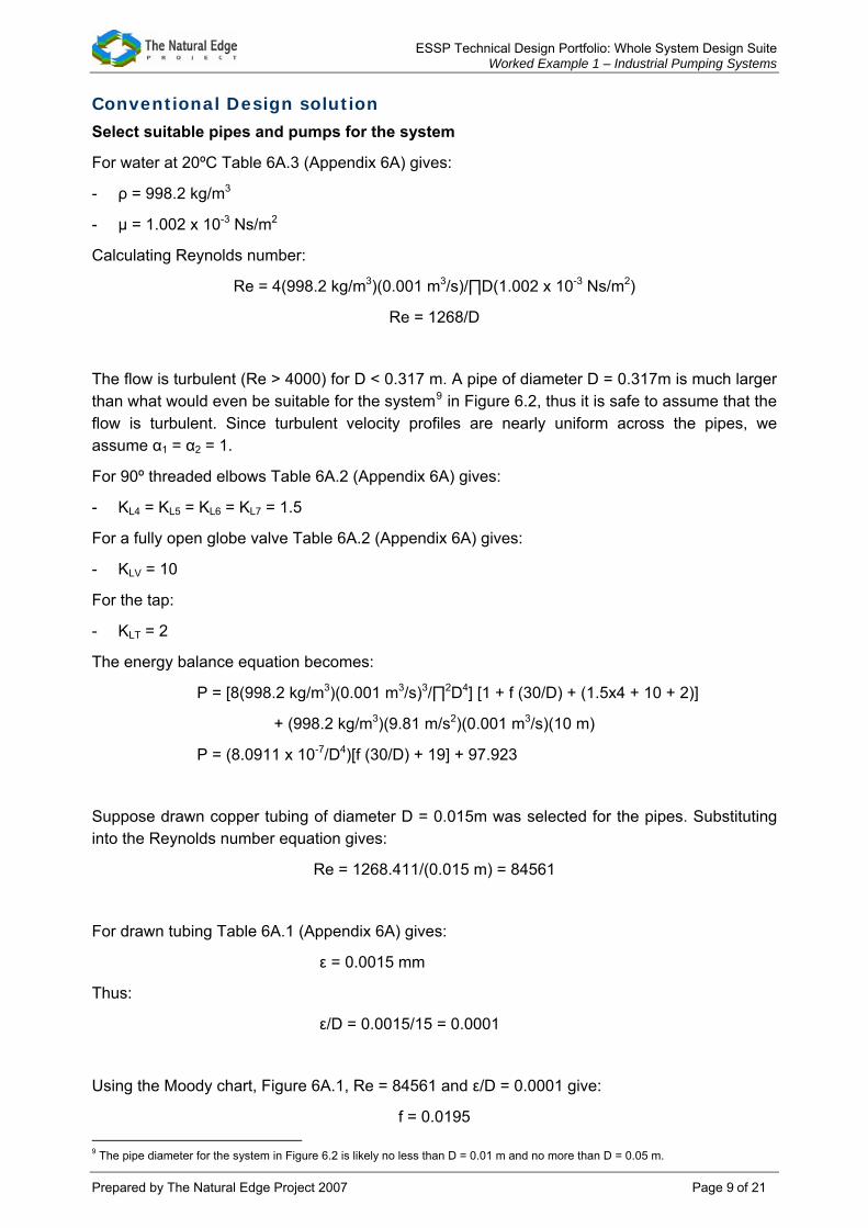
Select suitable pipes and pumps for the system

For water at 20ºC Table 6A.3 (Appendix 6A) gives:

- ρ = 998.2 kg/m3

- μ = 1.002 x 10-3 Ns/m2

Calculating Reynolds number:

Re = 4(998.2 kg/m3)(0.001 m3/s)/∏D(1.002 x 10-3 Ns/m2)

Re = 1268/D

The flow is turbulent (Re > 4000) for D < 0.317 m. A pipe of diameter D = 0.317m is much larger than what would even be suitable for the system9 in Figure 6.2, thus it is safe to assume that the flow is turbulent. Since turbulent velocity profiles are nearly uniform across the pipes, we assume α1 = α2 = 1.

For 90º threaded elbows Table 6A.2 (Appendix 6A) gives:

- KL4 = KL5 = KL6 = KL7 = 1.5

For a fully open globe valve Table 6A.2 (Appendix 6A) gives:

- KLV = 10

For the tap:

- KLT = 2

The energy balance equation becomes:

P = [8(998.2 kg/m3)(0.001 m3/s)3/∏2D4] [1 + f (30/D) + (1.5x4 + 10 + 2)]

+ (998.2 kg/m3)(9.81 m/s2)(0.001 m3/s)(10 m)

P = (8.0911 x 10-7/D4)[f (30/D) + 19] + 97.923

Suppose drawn copper tubing of diameter D = 0.015m was selected for the pipes. Substituting into the Reynolds number equation gives:

Re = 1268.411/(0.015 m) = 84561

For drawn tubing Table 6A.1 (Appendix 6A) gives:

ε = 0.0015 mm

Thus:

ε/D = 0.0015/15 = 0.0001

Using the Moody chart, Figure 6A.1, Re = 84561 and ε/D = 0.0001 give:

f = 0.0195 9 The pipe diameter for the system in Figure 6.2 is likely no less than D = 0.01 m and no more than D = 0.05 m.



Substituting D = 0.015 m and f = 0.0195 into the equation for pump power gives:

P = (8.0911 x 10-7/(0.015 m)4)[0.0195 (30/(0.015 m)) + 19] + 97.923 = 1025 W

That is, for the system in Figure 6.2, if drawn copper tubing of diameter D = 0.015 m is used for the pipes, then a pump of power P = 1025 W is required to generate an exit volumetric flow rate of Q = 0.001 m3/s.

From ‘Water pumps pricelist’ (Appendix 6B) we can select a pump model:

Waterco Hydrostorm Plus 15010 at P = 1119 W (1.5 hp)

From ‘Hard drawn copper tube (6M length)’ in ‘Kirby copper pricelist’ (Appendix 6C) we can select a pipe:

T24937 at D = 15 mm (5/8 in)

Calculate the cost of the system

For copper pipe T24937 ‘Hard drawn copper tube (6M length)’ in ‘Kirby copper pricelist’ (Appendix 6C) gives a cost of $57.12 per 6m. Therefore the cost of 30m of copper pipe is:

Pipe cost = ($57.12 per 6m)(30 m)/6 = $285.60

For standard radius 90º elbows of 15mm (5/8 in) diameter J00231 ‘copper fittings’ in the ‘Kirby copper pricelist’ (Appendix 6C) gives a cost of $2.34 each. Therefore the total cost of the elbows is:

Elbow cost = ($2.34)(4) = $9.36

For a globe valve of diameter 15mm (5/8 in), interpolating a ‘components pricelist’ (Appendix 6D) gives:

Estimated globe valve cost = $13 (US$10)

For a tap of exit diameter 0.015 m ‘components pricelist’ (Appendix 6D) gives:

Tap cost = $6.70

Installation costs for 8hrs at $65/hr gives:

Installation costs = ($65/hr)(8 hrs) = $520

10 Waterco (2004) Hydrostorm Plus Pool and Spa Pumps. Waterco, p 2. Available at http://www.waterco.com.au/brochures/ZZB0908_HydrostormPlus.pdf (accessed 11 July 2006). Waterco shows that this pump has a max Q = 400 l/min, whereas we require Q = 600 l/min (0.001m3/s). However, in practice, Q = 600 l/min (0.001m3/s) would be an unusually high flow rate for the system in Figure 6.2. Hence it is reasonable to ignore this relatively minor discrepancy because the system itself is not entirely practical.


http://www.waterco.com.au/brochures/ZZB0908_HydrostormPlus.pdf


For the Waterco Hydrostorm Plus 150 gives:

Pump cost = $616

Thus, the total capital cost of the system is:

Capital cost = $285.60 + $9.36 + $13 + $6.70 + $520 + $546

= $1451

To calculate running costs for the selected electrically powered pump, the following values are used:

- pump efficiency for an electrical pump: 47%11

- cost of electricity: $0.1/kWh (2006 price for large energy users)

For the Waterco Hydrostorm Plus 150 pump running at output power P = 1025 W, the monthly pump running costs for 12 hrs/day, 26 day/mth are:

Running cost = ($0.1/kWh)(1.025 kW)(12 hrs/day)(26 day/mth)/(0.47)

= $68/mth

11 ESPA (2000) SILENT Series; TYPHOON Series: Swimming pool pumps: Instruction Manual, Monarch Pool Systems, p 2. Available at http://www.monarchpoolsystems.com/manuals/PDF/Espa-manual.pdf (accessed 11 July 2006). This value is an approximation based on the data given by ESPA for the Silent 75M.


http://www.monarchpoolsystems.com/manuals/PDF/Espa-manual.pdf


Whole System Design Solution Is the conventional solution optimal for the whole system? What are the factors of the whole system that need to be considered? The conventional design solution was suboptimal for two reasons:

1. Ask the right questions

1. The pipe configuration introduced head losses that could be avoided, and

2. The selection procedure for pipe diameter, D, and pump power, P, did not address the whole system.

Redesign the pipes and pump system with less head loss

Items to consider:

- From Bernoulli’s equation, 4

1D

Power ∝ Increasing

diameter dramatically reduces power required

7. Review the system for potential improvements

- Can the system be designed with less bends? - Can the system be designed with more-shallow bends? - Is it worthwhile moving the plant equipment (machine press)? - Is an alternative pipe material more suitable? - Is there a more suitable valve? Do we even need a valve?

Figure 6.3. An alternative, Whole System Design configuration, which accommodates for the window and the machine press shown in Figure 6.1

Source: adapted from Munson, B.R., Young, D.F. and Okiishi, T.H. (1998), pp512, 522, 80012

12 Munson, B.R., Young, D.F. and Okiishi, T.H. (1998) Fundamentals of Fluid Mechanics, 3rd edn, Wiley & Sons, New York, pp512, 522, 800.



Select suitable pipes and pumps for the system

Since the conditions at point 1 and point 2 in Figure 6.3 are the same as in Figure 6.2, and a single pump and single pipe are used, the energy balance equation for the general solution is applicable:

P = (8ρQ3/∏2D4) [α2 + f (L/D) + Σ KLi] + ρgQz2

For 45º threaded elbows Table 6A.2 (Appendix 6A) gives:

- KL4 = KL5 = 0.4

For a fully open gate valve Table 6A.2 (Appendix 6A) gives:

- KLV = 0.15

For the tap:

- KLT = 2

The energy balance equation becomes:

P = [8(998.2 kg/m3)(0.001 m3/s)3/∏2D4] [1 + f (24/D) + (0.4x2 + 0.15 + 2)]

+ (998.2 kg/m3)(9.81 m/s2)(0.001 m3/s)(10 m)

P = (8.0911 x 10-7/D4)[f (24/D) + 3.95] + 97.923

Suppose, instead, a drawn copper pipe of diameter D = 0.03m (double the diameter in the conventional solution) was selected. Substituting into the Reynolds number equation gives:

Re = 1268.411/(0.03 m) = 42280

For drawn tubing13 Table 6A.1 (Appendix 6A) gives:

- ε = 0.0015 mm

Thus: ε/D = 0.0015/30 = 0.00005

Using the Moody chart, Figure 6A.1, Re = 42280 and ε/D = 0.00005 give:

- f = 0.0215

Substituting D = 0.03 m and f = 0.0215 into the equation for pump power gives:

P = (8.0911 x 10-7/(0.03 m)4)[0.0215 (24/(0.03 m)) + 3.95] + 97.923 = 119 W

13 Munson, B.R., Young, D.F. and Okiishi, T.H. (1998) Fundamentals of Fluid Mechanics, 3rd edn, Wiley & Sons, New York, p 492. Pipes of diameter 0.01-0.04m are available in a few different materials, including copper, steel and aluminium. Munson, Young and Okjishi suggest that drawn metal tubing, such as the copper pipes incorporated in the conventional solution, are the smoothest of the suitable pipes for the Design Challenge. Although plastic pipes are virtually frictionless, they are also generally larger than what is required, starting at diameters of about 0.05m (1 in).



That is, for the system in Figure 6.3, if drawn copper tubing of diameter D = 0.03 m is used for the pipes, then a pump of power P = 119 W is required to generate an exit volumetric flow rate of Q = 0.001 m3/s.

From ‘Water pumps pricelist’ we can select pump model:

Monarch ESPA Whisper 50014 at P = 370 W (0.5 hp)

From ‘Hard drawn copper tube (6M length)’ in ‘Kirby copper pricelist’ we can select pipe:

T22039 at D = 31.75 mm (1¼ in)

Is this the optimal solution for the whole system?

Consider the effect of other pipe diameters and pump powers

Other combinations of pipe diameter and pump power15 that suit the system can be selected in a similar way, as in Table 6.2:

3. Design and optimise the whole system

Table 6.2: Pump power calculated for a spectrum of pipe diameters

D (m) Re ε/D F P (W)

0.015 84561 0.0001 0.0195 660

0.02 63421 0.000075 0.0205 242

0.025 50736 0.00006 0.0210 148

0.03 42280 0.00005 0.0215 119

0.04 31710 0.0000375 0.0230 104

14 Monarch Pool Systems (n.d.) Whisper Series: Swimming Pool Pumps, Monarch Pool Systems, p 2. Available at http://www.monarchpoolsystems.com/products/Low%20Res%20PDFs/Whisper.pdf (accessed 13 July 2006). Monarch Pool Systems shows that this pump has a max Q = 160 l/min, whereas we require Q = 600 l/min (0.001m3/s). However, in practice, Q = 600 l/min (0.001m3/s) would be an unusually high flow rate for the system in Figure 6.2. Hence it is reasonable to ignore this relatively minor discrepancy because the system itself in not entirely practical. ‘Water Pumps Pricelist’ also shows two other pumps – little Giant Utility Sump 50500 and Flotec Waterfall/Utility FP0S1200X – that are better matched (with respect to power) to the system in Figure 6.3. However, these pumps are usually too small to be used in an application such as the system in Figure 6.3, and their flow rate of Q = 76 l/min (1200gph) is too much of a stretch to simply ignore. 15 Only system with diameter up to D = 0.04m are shown. At higher diameters the power savings become small. For example D = 0.05 m gives P = 102W; and D = 0.06 m gives 100W.


http://www.monarchpoolsystems.com/products/Low%20Res%20PDFs/Whisper.pdf


Calculate the cost of the system

The capital and running costs for each pipe and pump combination are shown in Table 6.3. The costs are calculated in a similar way as for the conventional solution. The efficiency of the Monarch ESPA Whisper 1000 is approximated at 42%16 and the efficiency of the Monarch ESPA Whisper 500 is approximated at 40%.17 The life cycle economic cost of each solution is estimated as the net present value (NPV) calculated over a life of 50 years and at a discount rate of 6%.

Table 6.3: Summary of system costs for a range of pump types and pipe diameter

D (m)

Pipes and components

cost P (W)

Pump selected

Pump cost

Total capital

cost

Running cost

Life cycle cost

(-NPV18)

0.015 $602 660 Monarch ESPA Whisper 1000

$357 $959 $49/mth $10,821


$331 $1076 $19/mth $4,873


$331 $1158 $12/mth $3,480


$331 $1245 $9/mth $3,112


$331 $1457 $8/mth $3,089

Table 6.3 shows that the solution with D = 0.015m has the lowest capital cost by a relatively small margin, but the highest life cycle cost by a factor of 2-3. Given the estimation errors in our calculations, the life cycle cost for the solution with D = 0.03 m is about the same as that for a system with D = 0.04 m. However, the capital cost is about $200 less and would therefore incur smaller economic stress up front.19 Hence, for the optimal pipe and pump combination for the system in Figure 6.3 we can select:

ESPA Whisper 500 pump at P = 370 W (0.5 hp)

T22039 hard drawn copper pipe at D = 31.75 mm (1¼ in)

16 ESPA (2000) SILENT Series; TYPHOON Series: Swimming pool pumps: Instruction Manual, Monarch Pool Systems, p 2. Available at http://www.monarchpoolsystems.com/manuals/PDF/Espa-manual.pdf (accessed 11 July 2006).This value is an approximation based on the data given by ESPA for the Silent 30M. 17 Ibid. This value is an approximation based on the data given by ESPA, which shows a trend of decreasing efficiency with decreasing power capacity. 18 Negative (-) values for NPV are actually costs. 19 Alternatively, the risk involved with spreading the system cost over a period where the economic situation can only be estimated may be a greater stress than having to pay more up front. Consequently, in this worked example either solution is as good as the other.




Summary: Performance Comparisons

A side-by-side comparison of the conventional design solution system and the Whole System Design (WSD) solution in Table 6.4 highlights the substantially different results that each approach achieves:

Table 6.4: Comparing the costs of the two solutions

Solution D (m)

Pipes and components

cost

P (W)

Pump cost

Total capital

cost

Running cost

Life cycle cost (-NPV)

Conventional 0.015 $835 1025 $616 $1451 $61/mth $15,129

WSD 0.03 $914 119 $331 $1245 $9/mth $3,112

The life cycle cost of the Whole System Design solution is about five-fold smaller than for the conventional solution. Since the capital costs of both solutions are similar, it is obvious that the cost savings for the Whole System Design solution arises from the lower required pumping power and hence running cost. This example demonstrates the dominance of running costs over capital costs – a relationship that is common for many resource consuming systems. The power reduction was made possible by the inclusion of two additional steps in the design and selection process:

1. Step 1: Redesign the pipes and pump system with less head loss, and

2. Step 2: Consider the effect of other pipe diameters and pump powers.

Step 1 optimised the system configuration and yielded system wide improvement, regardless of the pipe diameter selected. Even with the same pipe diameter as the conventional solution (D = 0.015 m), the Whole System Design solution has a 28% lower pipes and components cost; requires 36% less power; has a 34% lower capital cost; and comes in about 28% cheaper over its life, as shown in Figure 6.4.

Step 2 optimised the pipe diameter and pump selection process. Notably, the larger diameter pipes reduced the total required pumping power of the system. The second step resulted in a further 82% reduction in power and 71% reduction in life cycle cost, as shown in Figure 6.4.

In total, the Whole System Design solution uses 88% less power; costs 79% less over its life; and is cheaper to purchase and install than the conventional solution.



(a) Life cycle cost

(b) Capital cost and breakdown

(c) Pumping power

Figure 6.4. Comparing the effects of Step 1 and Step 2



Multiple benefits

A number of other benefits arise from designing the pumping system such that it is ‘short, fat, and straight’ rather than ‘long, thin and bent’:

4. Account for all measurable impacts

- More floor space is available – less piping covering the floors of industrial sites means more space is available to work in, as well as improving the safety of the work environment.

- More reliable operation – less bends and valves in piping reduces the likelihood of parts failing. Reducing friction in the piping means that less energy is lost to adding physical stress to the piping system, thereby increasing the life of the system. Since less power is required, the motor driving the pump doesn’t need to work as hard.

- Easier maintenance – with short and straight pipes, maintenance workers can get into the system with relative ease, as opposed to negotiating a maze of piping in the conventional solution.

- Better performance – A much greater percentage of energy used in the system is converted into useful work. A system that is more reliable and easy to maintain provides consistently high performance relative to conventional systems.



Factors to consider for larger systems

Extra considerations for larger pipes

The pipe sizes considered in this worked example can be installed and mounted without restriction. However, a few notes should be made about larger pipes:

- A structure design permit may be required before mounting the pipe to an existing structure. Attaining the permit may incur a cost.

- Large pipes are heavier and thus may require additional mounting support, which may incur a cost.

- Pipes larger than about 0.05m (2 in) diameter may require stress analysis to account for the effects of thermal expansion. Tables that suggest when stress analysis should be performed are available. The tables usually consider pipe diameter and fluid temperature.

- Long straight pipes experience more wall stress than shorter, bent pipes. Systems with long straight pipes can also result in higher forces and resulting moments on inertia on the fixed nozzles of equipment, especially when the endpoints of the system are under pressure (say in a tank as opposed to open air). In these cases, expansion joints and bellowed nozzles can be incorporated to an advantage, with the key consideration being to make bends as smooth as possible.

Site planning

In this worked example, it was assumed that reservoir A, the pump, and the tap were to remain where there were. Sometimes, the location of such features is arbitrary, as in the ‘Pipes and Pumps’ example in Natural Capitalism,20 so their location can be governed by the piping system. Other times, however, other factors can influence where these features as well as the pipes should be located. For example, a pipe and pump system can share many resources with other equipment and systems. These resources include shelter, electrical cable route, drainage systems, and access ways for maintenance. Accounting for these factors is an example of Step 3, ‘Design and optimise the whole system’ and Step 4, ‘Account for all measurable impacts’.

Larger cost reductions

In this worked example, the small amount of required pumping power21 did not lend itself to a good demonstration of pump capital cost savings. Table 6.3 shows that even though required pumping power fell by a factor of more than two between the solution where D = 0.02m and the solution where D = 0.04m, the same pump was used for all solutions and hence the pump capital cost was the same. In a larger system, the required pumping power falls over a larger range for which there is a variety of pumps that can be selected.

Internal combustion engine powered systems

Some moderate sized systems use pumps powered by internal combustion engines (ICE). The size of ICE pumps start at about 1.5 kW output power. They are usually cheaper to purchase but more expensive to run than the equivalent electric pump. Consequently, moderate sized ICE pump systems have even greater potential for cost savings.

To demonstrate, consider a conventional, ICE-powered system that requires 10kW of pumping power. We have shown that Whole System Design can reduce the pumping power of a conventional system by 88%. The 10kW conventional system can therefore be redesigned as a 20 Hawken, P., Lovins, A.B. and Lovins, L.H. (1999) Natural Capitalism: Creating the Next Industrial Revolution, Earthscan, London. 21 The optimised whole systems design solution required the same amount of power (119W) as a bright incandescent lamp.



1.2kW system, which means the 10kW ICE pump costing about $12,70022 can be replaced with a 1.5kW electric pump costing $616.23

Now, since the required pumping power is reduced by 88%, the running costs are then reduced by 88%. Furthermore, an additional saving arises since the electrical pump is at least twice as efficient as the ICE pump (20-26%24) while the cost per unit energy is about the same for electricity ($0.10/kWh for large energy users, $0.17 for domestic users) as it is for petrol ($0.14/kWh at $1.30 per litre).

Effectively, the lower power consumption of the Whole System Design solution makes viable solutions that bring with them additional benefits and that are otherwise too expensive.

To calculate the cost per unit energy of petrol, the following values are used:

- energy value of petrol: 34 MJ/litre25

- cost of petrol: $1.30/litre (2006 price at the pump)

The cost per unit energy for petrol is:

Cost per unit energy = ($1.30/litre)/(34,000,000 J/litre)

= 3.8235 x 10-8 $/J

Converting to units of $/kWh:

Cost per unit energy = [(3.8235 x 10-8 $/J)/(1 s)](1000 W/kW)(3600 s/hr)

= $0.14/kWh

22 ‘Water Pumps Pricelist’ gives details for a 10kW (13 hp) Fire 02.5F13K2V pump. 23 ‘Water Pumps Pricelist’ gives details for a 1.5kW (2 hp) Waterco Hydrostorm Plus 200 pump. 24 Evans, R., Sneed, R.E. and Hunt, J.H. (1996) Pumping plant performance evaluation, North Carolina Cooperative Extension Service. Available at http://www.bae.ncsu.edu/programs/extension/evans/ag452-6.html (accessed 27 June 2006). This value is an overestimate. The data is for an internal combustion engine only, and does not include any mechanical losses associated with the coupling of the engine to the pump or the pump itself. 25 Moorland School (n.d.) Petrol, http://www.moorlandschool.co.uk/earth/petrol.htm (accessed 27 June 2006).


http://www.bae.ncsu.edu/programs/extension/evans/ag452-6.html

http://www.moorlandschool.co.uk/earth/petrol.htm


References

ESPA (2000) SILENT Series; TYPHOON Series: Swimming pool pumps: Instruction Manual, Monarch Pool Systems. Accessed 11 July 2006. Available at http://www.monarchpoolsystems.com/manuals/PDF/Espa-manual.pdf.

Evans, R., Sneed, R.E. and Hunt, J.H. (1996) Pumping plant performance evaluation, North Carolina Cooperative Extension Service. Accessed 27 June 2006. Available at http://www.bae.ncsu.edu/programs/extension/evans/ag452-6.html.

Hawken, P., Lovins, A.B. and Lovins, L.H. (1999) Natural Capitalism: Creating the Next Industrial Revolution, Earthscan, London.

Monarch Pool Systems (n.d.) Whisper Series: Swimming Pool Pumps, Monarch Pool Systems. Accessed 13 July 2006. Available at http://www.monarchpoolsystems.com/products/Low%20Res%20PDFs/Whisper.pdf.

Moorland School (n.d.) Petrol. Accessed 27 June 2006. Available at http://www.moorlandschool.co.uk/earth/petrol.htm.

Munson, B.R., Young, D.F. and Okiishi, T.H. (1998) Fundamentals of Fluid Mechanics, 3rd edn, Wiley & Sons, New York.

Waterco (2004) Hydrostorm Plus Pool and Spa Pumps. Accessed 11 July 2006. Available at http://www.waterco.com.au/brochures/ZZB0908_HydrostormPlus.pdf.



http://www.bae.ncsu.edu/programs/extension/evans/ag452-6.html

http://www.monarchpoolsystems.com/products/Low%20Res%20PDFs/Whisper.pdf

http://www.moorlandschool.co.uk/earth/petrol.htm

http://www.waterco.com.au/brochures/ZZB0908_HydrostormPlus.pdf




Worked Example 1 – Appendix 6A July 2007




TDP ESSP Technical Design Portfolio: Whole System Design Suite Worked Example 1 – Appendix 6A

Appendix 6A Calculating the total energy balance

Symbol nomenclature

Symbol Description Unit

A Pipe cross sectional area m2

D Pipe diameter m

f Friction factor

g Acceleration due to gravity 9.81 m/s2

h Head loss m

KL Loss coefficient

L Pipe length m

p Pressure Pa

P Power W

Q Volumetric flow rate m3/s

R Universal gas constant 8.314 kJ/kmolK

Re Reynolds number

T Temperature K

V Average velocity m/s

z Height m

α Kinetic energy coefficient

γ Specific weight kN/m3

ε Equivalent roughness mm

μ Dynamic viscosity Ns/m2

ν Kinematic viscosity m2/s

ρ Density kg/m3

Prepared by The Natural Edge Project 2007 Page 2 of 15



Calculating the total energy balance

There are 4 kinds of energy changes associated with fluid flow through a pipe and pump system:

1. Pressure, kinetic energy and potential energy changes

2. Friction losses

3. Component losses

4. Pumping gains

1. Energy balance of a steady, inviscid (zero viscosity), incompressible flow in a frictionless pipe system (an ideal system) is governed by the Bernoulli equation, which indicates that the sum of the pressure, kinetic energy, and potential energy changes is constant along a streamline. The equation is given in terms of heads:

p/ρg + αV2/2g + z = constant along a streamline

For uniform velocity profiles α = 1. For non-uniform velocity profiles α > 1.

2. Friction head loss for a fully developed, steady, incompressible flow in a single pipe is given by the Darcy-Weisbach equation:

hF = f (L/D)(V2/2g)

The total friction head loss through all pipes in a pipe system is the sum of the individual friction losses.

Calculating the friction factor, f, depends on the type of flow. The Reynolds number is used to distinguish between laminar and turbulent flow:

Re = ρVD/μ

Reynolds number Type of fluid flow

Re < 2100 Laminar

2100 < Re < 4000 Transitional

Re > 4000 Turbulent

If the flow is laminar the friction factor is given by:

f = 64/Re

If the flow is turbulent the friction factor is a function of Re and the ratio ε/D, where ε is the equivalent roughness. Table 6A.1 gives values of ε for various types of pipe.



Table 6A.1: Equivalent Roughness for New Pipes

Pipe Equivalent roughness, ε

Feet Millimetres

Rivited steel 0.003 – 0.03 0.9 - 9.0

Concrete 0.001 – 0.01 0.3 – 3.0

Wood stave 0.0006 – 0.003 0.18 – 0.9

Cast iron 0.00085 0.26

Galvanised iron 0.0005 0.15

Commercial steel or wrought iron 0.00015 0.045

Drawn tubing 0.000005 0.0015

Plastic, glass 0.0 (smooth) 0.0 (smooth)

Source: Munson, B.R., Young, D.F. and Okiishi, T.H. (1998), p4921

1 Munson, B.R., Young, D.F. and Okiishi, T.H. (1998) Fundamental of Fluid Mechanics, 3rd edn, Wiley & Sons, New York, p492.


Figure 6A.1. The Moody Chart: Friction Factor as a function of Reynolds number and relative roughness for round pipes – the Moody Chart shows the relationship between f, Re and ε/D

Source: Munson, B.R., Young, D.F. and Okiishi, T.H. (1998) p4932

2 Ibid, p493.



Alternatively, t y chart:

1/√f = –2log10 [(ε/D)/3.7 + 2.51/(Re√f)]

3. Component head losses refer to losses associated with flow though components such as pipe contractions, expansions, bends, joins and valves. The component head loss through a single component is given by:

hC = KLV2/2g

The total head loss through all components in the system is the sum of the individual component losses. The loss coefficient, KL, depends on the type of component.

At a pipe contraction - where the upstream pipe cross sectional area, A1, is larger than the downstream pipe cross sectional area, A2 - KL is given by Figure 6A.2 for a rounded inlet edge and Figure 6A.3 for a sudden contraction.

he Colebrook formula is valid for the non-laminar range of the Mood

Figure 6A.2. Entrance loss coefficient as a function of rounding the inlet edge


Figure 6A.3: Loss coefficient for a sudden contraction

3 Ibid, p499.




Figure 6A.4 gives KL for vario umed to be infinite. us entrance conditions, where A1 is ass

Figure 6A.4. Entrance flow conditions and loss coefficient. (a) Re-entrant, KL = 0.8, (b) sharp-edged, KL = 0.5, (c) slightly rounded, KL = 0.2, (d) well-rounded, KL = 0.04.


At a sudden pipe expansion, where the upstream pipe cross sectional area, A1, is smaller than the downstream pipe cross sectional area, A2, KL is given by Figure 6A5.

Figure 6A.5: Loss coefficient for a sudden expansion


Alternatively, KL for a sudden expansion can be calculated using:

KL = (1- A1/A2) 2

Figure 6A.6 gives KL for various exit conditions, where A2 is assumed to be infinite.

4 Ibid, p500. 5 Ibid, p498. 6 Ibid, p500.



Figure 6A.6: Exit flow conditions and loss coefficient. (a) Re-entrant, KL = 1.0, (b) sharp-edged, KL = 1.0, (c) slightly rounded, KL = 1.0 (d) well-rounded, KL = 1.0.

Table 6A.2

7Source: Munson, B.R., Young, D.F. and Okiishi, T.H. (1998) p499

gives KL for flows through other types of components.

7 Ibid, p499.



Table 6A.2: Loss Coefficients for Pipe Components


8 Ibid, p505.



4. Pumping gains ref a single pump of power P pumping a fluid at average velocity V through a pipe of cross sectional area A is:

hP = P/ρgAV

The total pumping gain over all pumps in the system is the sum of the individual gains.

Total energy balance in terms of heads for a pipes and pumps system is given by combining the 4 sources of energy changes between point 1 and point 2 on a streamline:

p1/ρg + α1V12/2g + z1 + Σ hPi = p2/ρg + α2V2

2/2g + z2 + Σ hFi + Σ hCi

or

p1/ρg + α1V12/2g + z1 + Σ Pi/ρgAiVi

er to energy from a pump. The pumping head gain for

= p2/ρg + α2V22/2g + z2 + Σ fi (Li/Di)(Vi

2/2g) + Σ KLiVi2/2g

Other useful equations

γ = ρg

ν = μ/ρ

p = ρgh

Q = AV

For a circular pipe: A = ΠD2/4

Comparing pipe 1 with diameter D1 and pipe 2 with diameter D2:

hF1/hF2 = (D2/D1)5

For a perfect gas: p = ρRT



Useful resources

Table 6A.3: Physical Properties of Water (SI Units).

Source: Munson, B.R., Young, D.F. and Okiishi, T.H. (1998) p. 8539

9 Ibid, p853.



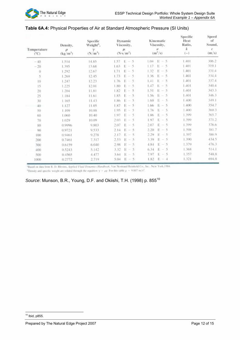
Table 6A.4: Physical Properties of Air at Standard Atmospheric Pressure (SI Units)

Source: Munson, B.R., Young, D.F. and Okiishi, T.H. (1998) p. 85510

10 Ibid, p855.



Table 6A.5: Conversion Factors from BG and EE Units to SI Units

Source: Munson, B.R., Young, D.F. and Okiishi, T.H. (1998)11

11 Ibid.



Table 6A.6: Conversion Factors from SI Units to BG and EE Units

Source: Munson, B.R., Young, D.F. and Okiishi, T.H. (1998)12

12 Ibid.




References

Munson, B., Young, D. and Okiishi, T. (1998) Fundamental of Fluid Mechanics, 3rd edn, Wiley & Sons, New York.




Worked Example 1 – Appendix 6B July 2007




TDP ESSP Technical Design Portfolio: Whole System Design Suite Worked Example 1 – Appendix 6B

Appendix 6B Water Pumps Price Lists

Pumpshop

http://www.pumpshop.com.au/(Accessed 11 August 2005)

Model Power Flow Port size Price Silent 50 370 W 40 mm AU$376.42 Silent 75 550 W 40 mm AU$389.18

Silent 100 750 W 40 mm AU$401.94

Hurlcon

Model Power Flow Port size Price LX300 0.33 hp 320 l/m @ 30kPa AU$497.42


http://www.pumpshop.com.au/



Model Power Flow Port size Price Whisper 500 0.5 hp 40 mm AU$330.99 Whisper 750 0.75 hp 40 mm AU$343.97

Whisper 1000 1 hp 40 mm AU$356.95

Speck

Model Power Flow Port size Price Magic 8 0.75 hp 160 l/m 40 mm AU$376.42

Magic 11 1 hp 220 l/m 40 mm AU$389.18

Waterco

Model Power Flow Port size Price Hydrostorm Plus 150 1.5 hp 50 mm AU$616 Hydrostorm Plus 200 2 hp 50 mm AU$662.20 Hydrostorm Plus 250 2.5 hp 50 mm AU$708.40 Hydrostorm Plus 300 3 hp 65 mm AU$839.30 Hydrostorm Plus400 4 hp 65 mm AU$985.60


Northern Tool and Equipment http://www.northerntool.com(Accessed 11 August 2005)

Little Giant Utility Sump

Model Power Total Head Flow Port size Price 505000 180 W 26.3 ft 1200 gph @ 1 ft 1 in US$79.99

Flotec Waterfall/Utility

Model Power Total Head Flow Port size Price FP0S1200X 180 W 1200 gph 0.5, 0.75, 1 in US$99.99 FP0S2300X 275 W 2300 gph 0.5, 0.75, 1 in US$119.99


http://www.northerntool.com/


Izumi

Model Power Total Head Flow Port size Price SMD-50HX 4 hp 50 ft 2000 gph

850 gph @ 33ft 2 in US$1149.99

SMD-80HX 5.5 hp 50 ft 2000 gph @ 33ft 3 in US$1349.99

NorthStar

Model Power Total Head Flow Port size Price 5.5 hp 187 ft 6960 gph 2 in US$599.99

SE 80 EX 6 hp 102 ft 15376 gph 3 in US$419.99



Gorman Rupp

Model Power Total Head Flow Port size Price 2P5A 5 hp 200 ft 7200 gph 2in US$499.99 2P5IR 6.5 hp 200 ft 8200 gph @ 20 ft 2in US$629.99

Davey

Model Power Total Head Flow Port size Price AK280 6 hp 302 ft 4800 gph 1.5 in US$999.99 AK282 9 hp 332 ft 7200 gph 1.5 in US$1799.99



A.Y. McDonald http://www.aymcdonald.com/(Accessed 11 August 2005)

Fire

Model Power Flow Port size Price 02.5F13K1V 13 hp 250 gpm 1.5 in US$10523 02.5F13K2V 13 hp 250 gpm 2.5 in US$9612 02.5F13K3V 23 hp 250 gpm 2.5 in US$11844


http://www.aymcdonald.com/

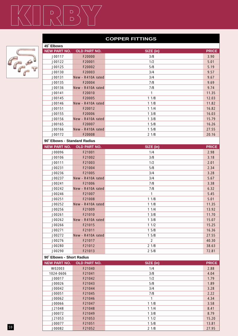
59

COPPER FITTINGS

NEW PART NO. OLD PART NO. SIZE (in) PRICE



45˚ Elbows

J00117 F20000 3/8 3.90J00122 F20001 1/2 5.01J00125 F20002 5/8 5.19J00130 F20003 3/4 9.57J00131 New - R410A rated 3/4 9.67J00135 F20004 7/8 9.69J00136 New - R410A rated 7/8 9.74J00141 F20010 1 11.35J00145 F20005 1 1/8 12.03J00146 New - R410A rated 1 1/8 11.82J00151 F20012 1 1/4 16.82J00155 F20006 1 3/8 16.03J00156 New - R410A rated 1 3/8 15.79J00165 F20007 1 5/8 16.26J00166 New - R410A rated 1 5/8 27.55J00172 F20008 2 1/8 20.16

90˚ Elbows - Standard Radius

J00096 F21001 1/4 2.98J00106 F21002 3/8 3.18J00111 F21003 1/2 2.01J00231 F21004 5/8 2.34J00236 F21005 3/4 3.28J00237 New - R410A rated 3/4 5.67J00241 F21006 7/8 3.38J00242 New - R410A rated 7/8 6.32J00246 F21007 1 5.45J00251 F21008 1 1/8 5.01J00252 New - R410A rated 1 1/8 11.35J00256 F21009 1 1/4 13.92J00261 F21010 1 3/8 11.70J00262 New - R410A rated 1 3/8 15.07J00266 F21015 1 1/2 15.25J00271 F21011 1 5/8 16.36J00272 New - R410A rated 1 5/8 27.55J00276 F21017 2 40.30J00280 F21012 2 1/8 38.63J00290 F21013 2 5/8 72.81

90˚ Elbows - Short Radius

W02003 F21040 1/4 2.881024-0606 F21041 3/8 4.04

J00017 F21042 1/2 1.79J00026 F21043 5/8 1.89J00042 F21044 3/4 3.28J00051 F21045 7/8 2.22J00062 F21046 1 4.34J00066 F21047 1 1/8 3.58J21048 F21048 1 1/4 8.41J00072 F21049 1 3/8 8.79J21053 F21053 1 1/2 15.20J00077 F21051 1 5/8 13.81J00082 F21052 2 1/8 27.95

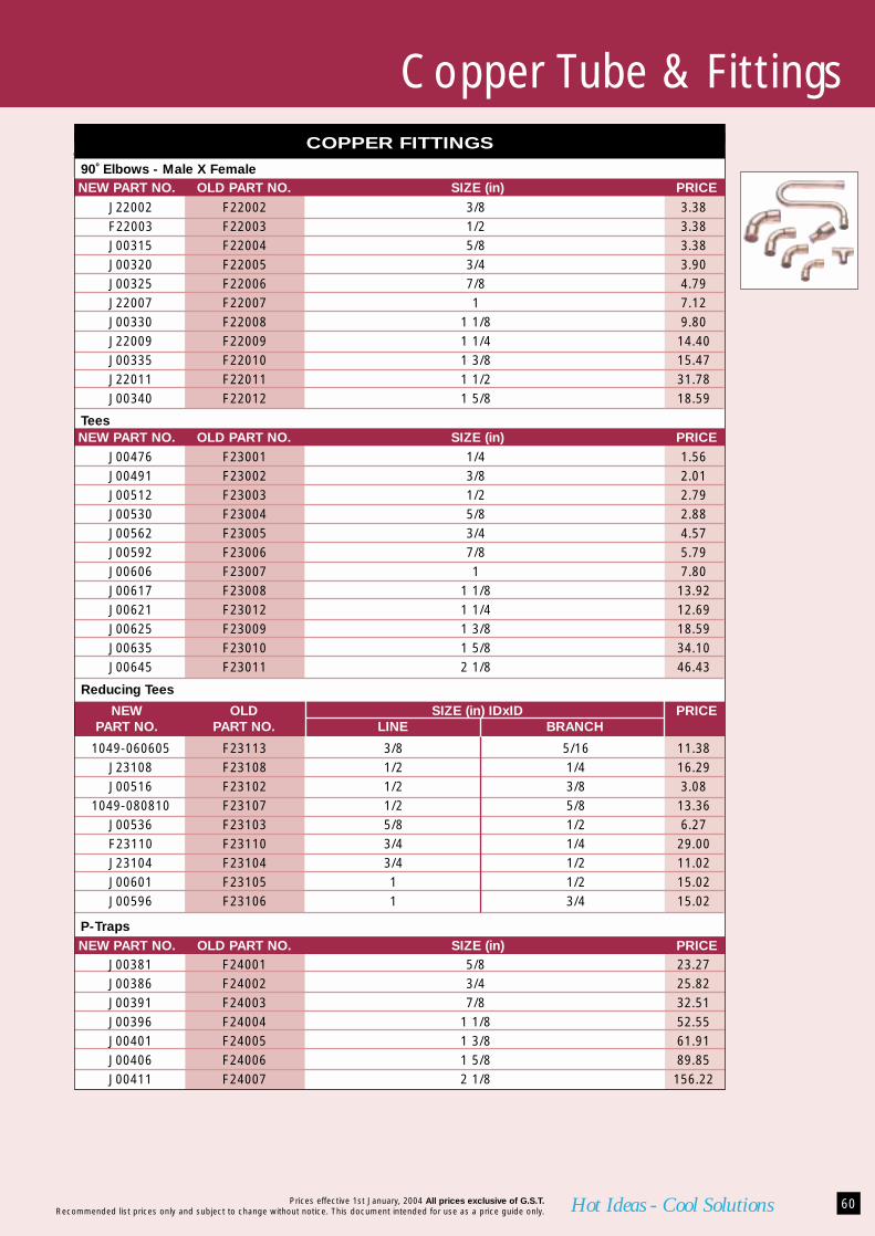
Copper Tube & Fittings

60Hot Ideas - Cool Solutions

COPPER FITTINGS



NEW OLD SIZE (in) IDxID PRICEPART NO. PART NO. LINE BRANCH

NEW PART NO. OLD PART NO. SIZE (in) PRICEP-Traps

J00381 F24001 5/8 23.27J00386 F24002 3/4 25.82J00391 F24003 7/8 32.51J00396 F24004 1 1/8 52.55J00401 F24005 1 3/8 61.91J00406 F24006 1 5/8 89.85J00411 F24007 2 1/8 156.22

Prices effective 1st January, 2004 All prices exclusive of G.S.T.Recommended list prices only and subject to change without notice. This document intended for use as a price guide only.

90˚ Elbows - Male X Female

J22002 F22002 3/8 3.38F22003 F22003 1/2 3.38J00315 F22004 5/8 3.38J00320 F22005 3/4 3.90J00325 F22006 7/8 4.79J22007 F22007 1 7.12J00330 F22008 1 1/8 9.80J22009 F22009 1 1/4 14.40J00335 F22010 1 3/8 15.47J22011 F22011 1 1/2 31.78J00340 F22012 1 5/8 18.59

Tees

J00476 F23001 1/4 1.56J00491 F23002 3/8 2.01J00512 F23003 1/2 2.79J00530 F23004 5/8 2.88J00562 F23005 3/4 4.57J00592 F23006 7/8 5.79J00606 F23007 1 7.80J00617 F23008 1 1/8 13.92J00621 F23012 1 1/4 12.69J00625 F23009 1 3/8 18.59J00635 F23010 1 5/8 34.10J00645 F23011 2 1/8 46.43

Reducing Tees

1049-060605 F23113 3/8 5/16 11.38J23108 F23108 1/2 1/4 16.29J00516 F23102 1/2 3/8 3.08

1049-080810 F23107 1/2 5/8 13.36J00536 F23103 5/8 1/2 6.27F23110 F23110 3/4 1/4 29.00J23104 F23104 3/4 1/2 11.02J00601 F23105 1 1/2 15.02J00596 F23106 1 3/4 15.02

61 Hot Ideas - Cool Solutions

COPPER FITTINGS


NEW PART NO. OLD PART NO. SIZE (in) IDxID PRICE

Prices effective 1st January, 2004 All prices exclusive of G.S.T.

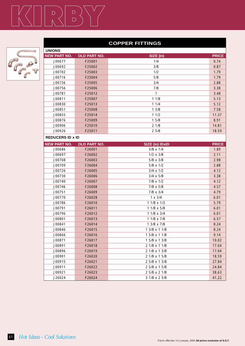
UNIONS

J00677 F25001 1/4 0.74J00692 F25002 3/8 0.87J00702 F25003 1/2 1.79J00716 F25004 5/8 1.79J00736 F25005 3/4 2.88J00756 F25006 7/8 3.38J00781 F25012 1 3.48J00811 F25007 1 1/8 5.13J00830 F25013 1 1/4 5.12J00851 F25008 1 3/8 7.58J00855 F25014 1 1/2 11.37J00876 F25009 1 5/8 8.91J00906 F25010 2 1/8 14.81J00926 F25011 2 5/8 18.59

REDUCERS ID x ID

J00686 F26001 3/8 x 1/4 1.89J00697 F26002 1/2 x 3/8 2.11J00708 F26003 5/8 x 3/8 2.98J00709 F26004 5/8 x 1/2 2.88J00726 F26005 3/4 x 1/2 4.12J00730 F26006 3/4 x 5/8 3.38J00740 F26007 7/8 x 1/2 4.12J00746 F26008 7/8 x 5/8 4.57J00751 F26009 7/8 x 3/4 4.79J00770 F26028 1 x 3/4 6.01J00786 F26010 1 1/8 x 1/2 5.79J00791 F26011 1 1/8 x 5/8 6.01J00796 F26012 1 1/8 x 3/4 6.01J00801 F26013 1 1/8 x 7/8 6.57J00841 F26014 1 3/8 x 7/8 8.24J00846 F26015 1 3/8 x 1 1/8 8.24J00866 F26016 1 5/8 x 1 1/8 9.14J00871 F26017 1 5/8 x 1 3/8 10.02J00891 F26018 2 1/8 x 1 1/8 17.04J00896 F26019 2 1/8 x 1 3/8 17.04J00901 F26020 2 1/8 x 1 5/8 18.59J00915 F26021 2 5/8 x 1 3/8 27.84J00911 F26022 2 5/8 x 1 5/8 24.84J00921 F26023 2 5/8 x 2 1/8 38.63J26024 F26024 3 1/8 x 2 5/8 41.22



BUSHINGS OD X ID

NEW PART NO. OLD PART NO. SIZE (in) OD(M)xID(F) PRICE

180˚ BENDS

NEW OLD SIZE (in) PRICEPART NO. PART NO. ID CENTRES

Y-PIECES (SWEAT)

NEW OLD SIZE (in) PRICEPART NO. PART NO. ID (A) ID (B)

Recommended list prices only and subject to change without notice. This document intended for use as a price guide only.

J00930 F27001 3/8 x 1/4 1.89J27002 F27002 1/2 x 1/4 1.99J00936 F27003 1/2 x 3/8 2.98J00940 F27004 5/8 x 3/8 2.88J00946 F27005 5/8 x 1/2 3.08J27006 F27006 3/4 x 1/2 3.87J00956 F27007 3/4 x 5/8 3.58J27008 F27008 7/8 x 1/2 4.67J00961 F27009 7/8 x 5/8 4.57J00966 F27010 7/8 x 3/4 4.57J00975 F27011 1 1/8 x 1/2 6.76J00976 F27012 1 1/8 x 5/8 5.45J00981 F27013 1 1/8 x 3/4 6.01J00986 F27014 1 1/8 x 7/8 9.80J27015 F27015 1 3/8 x 5/8 7.15J00996 F27016 1 3/8 x 7/8 10.35J01006 F27017 1 3/8 x 1 1/8 9.02J01021 F27018 1 5/8 x 7/8 10.14J01026 F27019 1 5/8 x 1 1/8 9.46J01031 F27020 1 5/8 x 1 3/8 14.36J01042 F27021 2 1/8 x 1 1/8 20.04J01046 F27022 2 1/8 x 1 3/8 18.59J01051 F27023 2 1/8 x 1 5/8 18.59

J28001 F28001 3/8 1 1/4 6.46J28004 F28004 5/8 2 8.94J28005 F28005 3/4 2 1/4 15.00J00462 F28006 7/8 2 1/2 16.69F28007 F28007 1 1/8 3 16.89J28009 F28009 1 5/8 4 3/8 29.00F28010 F28010 2 1/8 5 1/8 47.18

J01186 J01186 1/2 3/8 12.28J01187 F28101 5/8 1/2 29.62J28102 F28102 5/8 5/8 26.22J01188 F28103 3/4 5/8 29.62J01190 F28104 7/8 5/8 28.17J01191 F28105 7/8 7/8 32.18J28107 F28107 1 3/4 35.36


SOFT DRAWN COPPER TUBE

NEW OLD CONNECTION OD WALL THICKNESS ROLL LENGTH PRICEPART NO. PART NO. (in) (mm) (mm) GAUGE (m)

HARD DRAWN COPPER TUBE (6M LENGTH)

NEW OLD CONNECTION OD WALL THICKNESS PRICEPART NO. PART NO. (in) (mm) (mm) GAUGE

ACR TUBE

NEW OLD CONNECTION OD WALL THICKNESS ROLL LENGTH PRICEPART NO. PART NO. (in) (mm) (mm) GAUGE (m)

Prices effective 1st January, 2004 All prices exclusive of G.S.T.

T32263 C22S316 3/16 4.76 0.71 22 30 80.00T32336 C20S14 1/4 6.35 0.91 20 30 114.18T32522 C20S516 5/16 7.94 0.91 20 30 140.99T32662 C20S38 3/8 9.53 0.91 20 18 102.27T32930 C20S12 1/2 12.7 0.91 20 18 115.18T33090 C20S58 5/8 15.88 0.91 20 18 163.00T16850 New 5/8 15.88 1.02 R410A rated 18 170.00T33294 C20S34 3/4 19.05 0.91 20 18 176.00T76198 C20S78 7/8 22.22 0.91 20 18 255.17

T92029 C20H14 1/4 6.35 0.91 20 25.68T56847 C20H38 3/8 9.53 0.91 20 37.73T22527 C20H12 1/2 12.7 0.91 20 41.39T24937 C20H58 5/8 15.88 0.91 20 57.12T16870 New 5/8 15.88 1.02 R410A rated 62.00T88072 C20H34 3/4 19.05 0.91 20 61.31T16855 New 3/4 19.05 1.14 R410A rated 73.00T13862 C20H78 7/8 22.22 0.91 20 88.04T23515 New 7/8 22.22 1.63 R410A rated 149.25T60658 C20H1 1 25.4 0.91 20 96.95T73971 C20H118 1 1/8 25.58 0.91 20 105.34T14569 New 1 1/8 25.58 1.83 R410A rated 202.00T22039 C20H114 1 1/4 31.75 0.91 20 122.62T15237 C20H138 1 3/8 34.92 0.91 20 138.34T91987 C18H138 1 3/8 34.92 1.22 18 178.29T75980 New 1 3/8 34.92 2.03 R410A rated 279.00T15644 C20H112 1 1/2 38.1 0.91 20 149.35T32921 C20H158 1 5/8 41.28 0.91 20 162.46T16865 New 1 5/8 41.28 2.41 R410A rated 373.00T94960 C18H218 2 1/8 53.98 1.22 18 275.64T31976 C18H258 2 5/8 66.68 1.6 18 407.45

T59422 ZC20S14 1/4 6.35 0.76 21 15.24 57.32T55745 ZC20S38 3/8 9.52 0.81 21 15.24 85.98T54136 ZC20S12 1/2 12.7 0.81 21 15.24 97.67T52079 ZC20S58 5/8 15.88 0.89 20 15.24 136.83T63721 ZC20S34 3/4 19.05 0.89 20 15.24 149.08



COPPER SADDLES


PAIRCOIL - PRE INSULATED COPPER TUBE


Recommended list prices only and subject to change without notice. This document intended for use as a price guide only.

CSL025 T14001 1/4 0.52CSL031 T14025 5/16 0.52CSL037 T14002 3/8 0.52CSH50 T14003 1/2 0.52CSH062 T14004 5/8 0.59CSH075 T14005 3/4 0.52CSH087 T14006 7/8 1.05CSH112 T14007 1-1/8 1.88CSH100 T14020 1 0.66CSH125 T14021 1-1/4 1.88CSH137 T14008 1-3/8 1.69CSH150 T14022 1-1/2 1.85CSH162 T14009 1-5/8 1.88CSH200 T14023 2 2.02DCS502 T14010 1/2 x 1/4 1.05DCS623 T14011 5/8 x 3/8 1.15DCS-753 T14024 3/4 x 3/8 1.78

T99515 PC1438 1/4 & 3/8 20m roll 262.57T99525 PC1412 1/4 & 1/2 20m roll 328.77T99535 PC1458 1/4 & 5/8 20m roll 444.60T99545 PC3812 3/8 & 1/2 20m roll 400.47T99555 PC3858 3/8 & 5/8 20m roll 472.18T99565 PC3834 3/8 & 3/4 20m roll 546.10T99575 PC1234 1/2 & 3/4 20m roll 606.78


CAPILLARY SERVICE PACKS

NEW OLD LENGTH ID PRICEPART NO. PART NO. (m) (mm) (in)

Prices effective 1st January, 2004 All prices exclusive of G.S.T.Recommended list prices only and subject to change without notice. This document intended for use as a price guide only.

CAPILLARY TUBE IN ROLLS

NEW OLD LENGTH ID OD PRICEPART NO. PART NO. (m) (mm) (in) (mm) (in)

30CAP0.66X1.72A T12001 30 0.66 0.026 1.72 0.68 136.00T12020 T12020 100 0.66 0.026 1.72 1.22 182.00

30CAP0.80 T12002 30 0.8 0.031 2.06 0.081 141.0030CAP0.90 T12003 30 0.9 0.035 2.18 0.086 146.00

T12004 T12004 30 1 0.039 2.28 0.09 140.0030CAP1.10 T12005 30 1.1 0.043 2.16 0.085 140.00

30CAP1.20A T12006 30 1.2 0.047 2.26 0.089 143.0030CAP1.30X2.58A T12007 30 1.3 0.051 2.58 0.102 193.00

30CAP1.50 T12008 30 1.5 0.059 2.28 0.111 158.0030CAP1.62 T12009 30 1.62 0.064 2.94 0.116 215.0030CAP1.78 T12010 30 1.78 0.07 3.1 0.122 225.00

100CAP1.78X3.10 T12025 100 1.78 0.07 3.1 0.122 434.0030CAP2.04X3.44A T12012 30 2.04 0.08 3.44 0.135 232.00

SP1 SP1 3660 0.66 0.026 17.05SP2 SP2 3660 0.8 0.031 17.05SP3 SP3 3660 0.9 0.033 17.05SP4 SP4 4270 1.1 0.043 17.05

SP4.5 SP4.5 4270 1.2 0.047 19.88SP5 SP5 4270 1.3 0.051 17.05SP6 SP6 3660 1.4 0.055 17.05

SP6.5 SP6.5 3660 1.5 0.059 22.67SP7 SP7 3050 1.62 0.064 17.05SP8 SP8 3660 1.78 0.07 17.05SP9 SP9 2750 1.9 0.075 17.05SP10 SP10 3050 2.04 0.08 17.05SP11 SP11 3660 2.24 0.088 17.05

VIBRATION ELIMINATORS

NEW OLD TO FIT COPPER TUBING (in) O/ALL MAX PRICEPART NO. PART NO. ACTUAL NOMINAL FLEX TUBING LENGTH WORKING

OD ID ID (mm) PRESSURE kPaVAF3 VAF3 3/8 1/4 3/8 210 3102 48.51VAF4 VAF4 1/2 3/8 3/8 229 3102 48.51VAF5 VAF5 5/8 1/2 1/2 248 3102 55.00VAF7 VAF7 3/4 5/8 3/4 286 3033 78.00VAF8 VAF8 7/8 3/4 3/4 292 3033 78.00VAF9 VAF9 1 1/8 1 1 330 2620 95.00VAF10 VAF10 1 3/8 1 1/4 1 1/4 375 2758 132.00VAF11 VAF11 1 5/8 1 1/2 1 1/2 432 2758 189.00VAF82 VAF82 2 1/8 2 2 508 2690 326.00VAF83 VAF83 2 5/8 2 1/2 2 1/2 610 2344 660.00

Tell




Worked Example 1 – Appendix 6D July 2007




TDP ESSP Technical Design Portfolio: Whole System Design Suite Worked Example 1 – Appendix 6D

Appendix 6D Water Pumps Price Lists

A.Y.McDonald


(Accessed 11 August 2005)

Globe Valve 2021

Diameter Price ¼ in US$8.72 3/8 in US$8.72 ½ in US$9.20 ¾ in US$10.911 in US$16.261 ¼ in US$26.371 ½ in US$32.532 in US$56.11

Swing check valve 2050T

Diameter Price ½ in US$6.53 ¾ in US$8.19 1 in US$11.47 1 ¼ in US$16.46 1 ½ in US$22.67 2 in US$35.25 2 ½ in US$71.17 3 in US$95.94 4 in US$158.49

Angle Sillock 2014

Diameter Price ½ in US$3.93 ¾ in US$5.05




Wet Earth http://www.wetearth.com.au

(Accessed 11 August 2005)

PVC Ball Valve Threaded

Diameter Price 15mm $3.82 20mm $4.35 25mm $6.10 32mm $7.55 40mm $12.96 50mm $16.01

Brass Gate valve


Bronze Ball Valve


Tap Brass (Hose Cock)

Diameter Price15mm Male $6.7920mm Male $7.48


http://www.wetearth.com.au/


Galvanised Hex Nipple


Galvanised Threaded Elbow

Diameter Price15mm $1.0820mm $1.5925mm $2.3932mm $3.4240mm $4.7850mm $7.24

Galvanised Threaded Socket


Galvanised Threaded Tee

Diameter Price15mm $1.5420mm $2.1825mm $3.4532mm $5.0940mm $6.3850mm $9.58



Brass Hex Nipple

Diameter Price 15mm $1.39 20mm $2.08 25mm $2.92

Brass Female Tee

Diameter Price15mm $3.5220mm $5.09

Brass Elbow

Diameter Price 15mm Female $3.52 20mm Female $5.36 20mm Male/Female $4.39


Whole System Design Suite - research.qut.edu.au · and arbitrary spot, and the pipe fitter is then...

Documents

Transcript of Whole System Design Suite - research.qut.edu.au · and arbitrary spot, and the pipe fitter is then...