€¦ · Web viewHave you ever been in contact with anyone who suffers from TB?

Who Suffers from Indoor Air Pollution? Evidence from Bangladesh
Susmita Dasgupta* Mainul Huq
M. Khaliquzzaman Kiran Pandey
David Wheeler
Development Research Group World Bank
World Bank Policy Research Working Paper 3428, October 2004 The Policy Research Working Paper Series disseminates the findings of work in progress to encourage the exchange of ideas about development issues. An objective of the series is to get the findings out quickly, even if the presentations are less than fully polished. The papers carry the names of the authors and should be cited accordingly. The findings, interpretations, and conclusions expressed in this paper are entirely those of the authors. They do not necessarily represent the view of the World Bank, its Executive Directors, or the countries they represent. Policy Research Working Papers are available online at http://econ.worldbank.org.
* Authors’ names in alphabetical order. We would like to express our appreciation to the field survey team of the Development Policy Group, for their excellent air-quality monitoring work under difficult conditions. We are also grateful to Kseniya Lvovsky, Maureen Cropper, Douglas Barnes, Bart Ostro and Paul Martin for useful comments and suggestions. Financial support for this study has been provided by Trust Funds through the Knowledge for Change Program of the World Bank’s Development Economics Vice-Presidency, and by the Development Research Group.
Pub
lic D
iscl
osur
e A
utho
rized
Pub
lic D
iscl
osur
e A
utho
rized
Pub
lic D
iscl
osur
e A
utho
rized
Pub
lic D
iscl
osur
e A
utho
rized

2
Abstract In this paper, we investigate individuals’ exposure to indoor air pollution (IAP). Using new survey data from Bangladesh, we analyze exposure at two levels: differences within households attributable to family roles, and differences across households attributable to income and education. Within households, we relate individuals’ exposure to pollution in different locations during their daily round of activity. We find high levels of exposure for children and adolescents of both sexes, with particularly serious exposure for children under 5. Among prime-age adults, we find that men have half the exposure of women (whose exposure is similar to that of children and adolescents). We also find that elderly men have significantly lower exposure than elderly women. Across households, we draw on results from our previous paper (Dasgupta, et al., 2004), which relate pollution variation across households to choices of cooking fuel, cooking locations, construction materials and ventilation practices. We find that these choices are significantly affected by family income and adult education levels (particularly for women). Overall, we find that the poorest, least-educated households have twice the pollution levels of relatively high-income households with highly-educated adults. Overall, we find that young children and poorly-educated women in poor households face pollution exposures that are four times those for men in higher-income households organized by more highly-educated women. In our previous paper, we recommended feasible changes in cooking locations, construction materials and ventilation practices that could greatly reduce average household pollution levels. In this paper, we consider measures for narrowing the exposure gap among individuals within households. We focus particularly on changes for infants and young children, since they suffer the worst mortality and morbidity from indoor air pollution, but our findings also apply to women and adolescents. Our recommendations for reducing their exposure are based on a few simple, robust findings: Hourly pollution levels in cooking and living areas are quite similar because cooking smoke diffuses rapidly and nearly-completely into living areas. However, outdoor pollution is far lower. At present, young children are only outside for an average of 3 hours per day. For children in a typical household, pollution exposure can be halved by adopting two simple measures: increasing their outdoor time from 3 to 5 or 6 hours per day, and concentrating outdoor time during peak cooking periods. We recognize that weather and other factors may intervene occasionally, and that child supervision outdoors may be difficult for some households. However, the potential benefits are so great that neighbors might well agree to pool outdoor supervision once they became aware of the implications for their children’s health.

3
1. Introduction
Indoor air pollution from burning wood, animal dung and other biofuels is a major cause of acute
respiratory infections (ARI), which constitute the most important cause of death for young children in
developing countries (Murray and Lopez, 1996). Acute lower respiratory infection (ALRI), the most
serious type of ARI, is often associated with pneumonia (Kirkwood et al., 1995). ALRI accounts for
20% of the estimated 12 million annual deaths of children under five, and about 10% of perinatal
deaths (WHO, 2001; Bruce, 1999). Nearly all of these deaths occur in developing countries, with the
heaviest losses in Asia (42% of total deaths) and Africa (28%) (Murray and Lopez, 1996). Through its
effect on respiratory infections, indoor air pollution (IAP) is estimated to cause between 1.6 and 2
million deaths per year in developing countries (Smith, 2000). Most of the dead are in poor
households and approximately 1 million are children (Smith, 1993; Smith, et al., 1993; Smith and
Mehta, 2000). Table 1 provides estimates of health damage from IAP by region.
Table 1: Annual Disease Burden From Indoor Air Pollution (Early 1990’s)
Source: World Bank (2002), drawing on Smith and Mehta (2000) and Von Schrinding, et al., (2001)
The size of IAP’s estimated impact has prompted the World Bank (2001) and other international
development institutions to identify reduction of indoor air pollution as a critical objective for the
coming decade. The current scientific consensus is that most respiratory health damage comes from
1 DALYs, or disability-adjusted life years, combine life-years lost from premature death and fractional years of healthy life lost from illness and disability (Murray and Lopez 1996).
Region Deaths (‘000)
Illness Incidence (‘000,000)
DALYs1 (‘000,000)
China 516.5 209.7 9.3 India 496.1 448.4 16.0 Sub-Saharan Africa 429.0 350.7 14.3 Other Asia & Pacific Islands 210.7 306.4 6.6 Mid-East and North Africa 165.8 64.2 5.6 Latin America & Caribbean 29.0 58.2 0.9 Total 1,800.0 1,400 .0 53.0

4
inhalation of respirable particles whose diameter is less than 10 microns (PM10), and recent attention
has focused particularly on fine particles (PM2.5).
In a previous paper, we analyzed variations in average IAP levels across Bangladeshi households
(Dasgupta, et al., 2004). We found that common variations in fuel use, cooking locations, construction
materials and ventilation characteristics lead to large differences in IAP. Non-fuel characteristics are
so influential that some households using “dirty” biomass fuels have PM10 concentrations comparable
to those in households using clean fuels such as liquid natural gas. Under adverse conditions, on the
other hand, Bangladeshi households using dirty fuels can experience 24-hour average PM10
concentrations as high as 800 ug/m3.
Such concentrations are far higher than outdoor PM10 levels considered dangerous for public
health in industrial societies (Galassi et al., 2000). In those societies, however, use of clean fuels is so
pervasive that attention focuses on outdoor pollution. In biofuel-using Bangladeshi households,
particularly in rural areas, the calculus is often reversed: Indoor air pollution (IAP) may be much
worse than outdoor pollution, and health risks may be severe for household members who are exposed
to IAP for long periods during the day.
In this paper, we use our survey data to estimate the incidence of IAP exposure for family
members by age-sex group, with a particular focus on young children. We investigate the two major
sources of differential exposure: individuals’ time spent in different locations (cooking areas, living
areas and outside), and hourly fluctuations in pollution from cooking. We also assess the effect of
parents’ income and education on average household pollution levels.
The remainder of the paper is organized as follows. In Sections 2-5 we study the sources of
variation in individuals’ exposure to pollution within households. The four sections analyze
individuals’ daily location patterns, their interaction with daily cycles in pollution from cooking, the

5
implications for pollution exposure, and some possible remedies for the most vulnerable family
members (particularly young children). Section 6 compares our results with those in a recent study for
India. In Section 7, we assess the effects of income and adult education on both determinants of
exposure: average pollution levels across households, and patterns of activity within households.
Section 8 provides a summary and conclusions.
2. Daily Location Patterns in Bangladeshi Households
Within households, individuals’ pollution exposure may vary significantly because they spend
very different amounts of time in cooking areas, living areas, and outside the house. Table 2 reports
average daily hours in the three locations for a representative sample of 4,612 individuals drawn from
600 households in rural, peri-urban and urban areas of seven Bangladeshi regions (Figure 1): Rangpur
(491 individuals) in the Northwest, Sylhet (578) in the Northeast, Rajshahi (491) and Jessore (490) in
the West, Faridpur (497) and Dhaka (1,493) in the Center, and Cox’s Bazar (572) in the Southeast.
Table 2 present statistics by sex, because gender roles are quite different in Bangladeshi
households. Among age groups, we distinguish infants (age 0-1) and young children (age 1-5)
because they are most vulnerable to air pollution, and most tied to their mothers’ patterns of activity.
We divide school-age youths into two groups with different patterns of school attendance that may
have implications for exposure to indoor pollution: students 6-8 years of age, who attend school in the
morning (9:00 a.m. – 12:00 a.m.), and students 9-19 years of age who attend from midday until late
afternoon (11:30 a.m. – 4:30 p.m.). We divide adults into prime-age (20-60) and older (60+)
categories.
Table 2 shows that time-location patterns are very similar for infants of both sexes. They spend
relatively short periods in cooking areas (1 hour per day), very long periods in living areas (20
hours/day), and the residual time (3 hours) outside the house. Infants spend more time indoors than
6
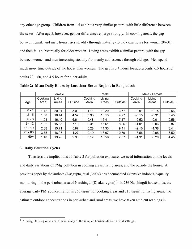
any other age group. Children from 1-5 exhibit a very similar pattern, with little difference between
the sexes. After age 5, however, gender differences emerge strongly. In cooking areas, the gap
between female and male hours rises steadily through maturity (to 3.6 extra hours for women 20-60),
and then falls substantially for older women. Living areas exhibit a similar pattern, with the gap
between women and men increasing steadily from early adolescence through old age. Men spend
much more time outside of the house than women: The gap is 3.4 hours for adolescents, 6.5 hours for
adults 20 – 60, and 4.5 hours for older adults.
Table 2: Mean Daily Hours by Location: Seven Regions in Bangladesh
3. Daily Pollution Cycles
To assess the implications of Table 2 for pollution exposure, we need information on the levels
and daily variations of PM10 pollution in cooking areas, living areas, and the outside the house. A
previous paper by the authors (Dasgupta, et al., 2004) has documented extensive indoor air-quality
monitoring in the peri-urban area of Narshingdi (Dhaka region).2 In 236 Narshingdi households, the
average daily PM10 concentration is 260 ug/m3 for cooking areas and 210 ug/m3 for living areas. To
estimate outdoor concentrations in peri-urban and rural areas, we have taken ambient readings in
2 Although this region is near Dhaka, many of the sampled households are in rural settings.
Female Male Male - Female
Age Cooking
Area Living Areas
Outside
Cooking Area
Living Areas
Outside
Cooking Area
Living Areas
Outside
0 - 1 1.12 20.04 3.01 1.11 19.29 3.57 -0.01 -0.75 0.562 - 5 1.08 18.44 4.52 0.93 18.13 4.97 -0.15 -0.31 0.456 - 8 1.01 16.40 6.61 0.48 16.41 7.17 -0.52 0.01 0.56
9 - 12 1.32 15.55 7.19 0.31 15.61 8.06 -1.01 0.06 0.8713 - 19 2.38 15.71 5.97 0.28 14.33 9.41 -2.10 -1.38 3.4420 - 60 3.75 16.05 4.27 0.19 13.07 10.79 -3.56 -2.98 6.52
60+ 1.48 19.76 2.93 0.17 16.56 7.37 -1.31 -3.20 4.45

7
Figure 1: Survey Areas in Bangladesh

8
Narshingdi (8 monitoring points), and rural areas of Jessore (16 points) and Rangpur (11 points).
Average outdoor concentrations in the three locations are 36, 48, and 62 ug/m3, respectively. The
overall average for 35 monitoring points is 50 ug/m3, which we have adopted as our estimate of
outdoor pollution for this exercise.
In the previous paper, we have shown that pollution generated in cooking areas diffuses almost
immediately into living areas.3 As a result, pollution in both areas exhibits strong pollution cycles in
response to fuel combustion for cooking. Drawing on information from continuous, 24-hour
monitoring of PM10 in 27 households in Narshingdi, Figure 2 displays a typical daily pollution cycle as
a 24-hour plot of the ratio of the hourly mean PM10 concentration to the daily mean concentration.4
Its distinguishing features include two peaks during morning and evening cooking times, when
pollution rises to over 3 times the daily average, and extensive periods in the afternoon and evening
when pollution is substantially lower than the daily average. Daily indoor pollution cycles are also
reflected in outdoor ambient cycles, as many houses emit cooking smoke. Figure 3 illustrates a typical
ambient cycle, drawn from 24-hour monitoring at 7 points in rural villages of Jessore and Rangpur.5
We combine mean indoor and outdoor pollution concentrations with the hourly ratios in Figures 2 and
3 to produce Table 3, which provides hourly estimates of PM10 in cooking areas, living areas and
outside the house.
3 For illustrations of the close relationship, see Dasgupta, et al. (2004), Figure 2, p. 12. 4 Of course, households differ significantly in the timing of daily peaks; some have three rather than two, and there are also significant differences in peak levels and change gradients. Figure 2 represents the central tendency in the observed patterns for 27 households.. 5 This cycle is clearly different from the cycle in Figure 2, for two apparent reasons. First, the outdoor cycle reflects the combined effect of fuel-burning in many households, whose daily cycles reach peaks at different times, and at different PM10 emissions intensities. However, this does not explain the large difference in the relative size of the two outdoor peaks, as compared with rough parity for the indoor peaks. Since the outdoor pattern is reproduced across several widely-separated monitoring points, we hypothesize that different atmospheric conditions lead to more pronounced accumulation and duration of suspended particulates in the evening. Alternatively, preparation of evening meals may cluster more tightly in time, leading to more concentrated loading of PM10 in the evening. Future research may shed more light on this phenomenon.

9
Figure 2: Daily PM10 Pattern for Cooking and Living Areas
Figure 3: Daily Ambient (Outdoor) Pollution Pattern in Rural Villages
0.0
0.5
1.0
1.5
2.0
2.5
12:00 AM 4:00 AM 8:00 AM 12:00 PM 4:00 PM 8:00 PM 12:00 AMTime
PM10
Rel
ativ
e to
Mai
n Da
ily P
M10
0.0
0.5
1.0
1.5
2.0
2.5
3.0
3.5
12:00 AM 4:00 AM 8:00 AM 12:00 PM 4:00 PM 8:00 PM 12:00 AMTime
PM10
Rel
ativ
e to
Mea
n D
aily
PM
10

10
Table 3: Daily PM10 Concentrations, by Location
Time
Kitchen
Living Area
Ambient
12:00 AM 78 63 40 1:00 AM 78 63 35 2:00 AM 78 63 37 3:00 AM 78 63 39 4:00 AM 78 63 41 5:00 AM 142 114 42 6:00 AM 257 207 47 7:00 AM 466 376 57 8:00 AM 845 683 44 9:00 AM 568 459 33
10:00 AM 382 308 28 11:00 AM 257 207 33 12:00 PM 173 139 39
1:00 PM 116 94 37 2:00 PM 78 63 34 3:00 PM 78 63 40 4:00 PM 78 63 37 5:00 PM 257 207 36 6:00 PM 845 683 66 7:00 PM 525 424 101 8:00 PM 326 263 88 9:00 PM 202 163 72
10:00 PM 126 101 50 11:00 PM 78 63 46
To interpret these results, it is useful to note that India’s 24-hour standard for rural exposure to
PM10 is 100 ug/m3.6 Over the daily cycle, outdoor pollution only rises to this level during one hour in
the early evening (around 7:00 p.m.). However, the standard is exceeded in the indoor cooking area
for 15 hours per day, and in living areas for 14 hours. During peak cooking periods, the PM10
concentrations rise to 845 ug/m3 in the cooking area and 683 ug/m3 in the living areas.
6 Bangladesh does not seem to have an equivalent standard, but similar conditions in the two countries make the Indian standard relevant in this context.

11
4. Daily Exposure for Different Household Members
We combine the information in Tables 2 and 3 to produce estimates of daily average PM10
exposure by age-sex group. To incorporate our hourly estimates for PM10 concentrations in cooking,
living and outside areas, we adopt a set of conventions for assigning family members to locations
during the 24-hour cycle. We provide a complete accounting of assignments for all age-sex groups in
Appendix 1. We assume that infants and children 0-5 spend their single hour in the cooking area
during the morning peak cooking time. We assume that women spend their cooking-area time during
peak cooking periods, and that young children have their outside time during the mid-afternoon.
For older children, part of outside time reflects schooling schedules; we assume that the balance
is devoted to play in the mid-late afternoon. Men’s outside work times lie in the interval 7:00 AM –
6:00 PM, with total hours reflecting the totals in Table 2. After accounting for cooking-area and
outside times, all family members are assigned to inside living areas for periods that match the totals
in Table 2. We compute daily exposure for members of each age-sex group by adding the 24 hourly
PM10 concentrations for their assigned locations and calculating the mean concentration. Table 4
presents the results.
To check the general validity of our estimates for a typical household, we replicate our approach
236 times, using the mean PM10 concentration for each household monitored by our study. These
concentrations vary widely, for reasons explored in our previous paper (Dasgupta, et al., 2004). We
average the results and present them alongside the typical household results in Table 4.

12
Table 4: Daily Average PM10 Exposure by Age and Gender*
Typical Household**
236 Monitored Households***
Age Female Male Female Male 0-1 216 214 209 195 1-5 212 212 199 192 6-8 173 172 156 163 9-19 207 174 196 194 20-60 227 116 221 118 60+ 220 161 264 188
* Outdoor PM10 = 50 ** PM10 concentrations: cooking area 260; living area 210 *** Averages for 236 separate calculations using monitored PM10 levels
Differences in the two sets of results stem from variations in average pollution levels, household
age-sex compositions, and time allocations by household members in the full set of monitored
households. We present the results for the typical household in order to display exposure variations
when inside/outside pollution concentrations and individuals’ time allocations are held constant. In
any case, the two sets of results are quite similar. The most striking finding is the high exposure --
around 200 -- for infants and children, regardless of gender. Exposures for student-age individuals (6-
19) are somewhat lower (although still quite high), and also similar for both sexes. The real gender-
based divergence occurs among adults, with women’s exposures nearly twice those for men in the age
group 20-60, and about 40% higher for older women (over 60).
Table 4 indicates that only adult males aged 20-60 have daily PM10 exposures low enough to
approach the Indian standard (100 ug/m3). All other household members have significantly higher
exposure levels, and the youngest children of both sexes have exposures that are among the most
dangerous. Mortality from respiratory disease among children in this age range attests to the potent
impact of such pollution levels.
Two features of our results warrant particular scrutiny. First, although attention has traditionally
focused on pollution in cooking areas, our results suggest that simultaneous pollution in living areas is

13
the true culprit. This is particularly true for young children, who spend only one hour per day in
cooking areas, on average. Living-area pollution is only moderately below cooking-area pollution and
follows the same cycle, so most daily inhalation of particulates occurs in the living areas. Adult males
have lower exposures simply because they are out of the house for many more hours per day.
Second, we should qualify our results with a cautionary note about the impact of very intense
pollution on women and children during peak cooking periods. It is possible that peak pollution
during a few hours per day causes disproportionate health damage. Currently-available scientific
evidence suggests that health damage is associated with daily average exposure levels, not peak hourly
exposures. However, the evidence is far from conclusive, and it is mostly derived from research on
outdoor pollution effects in industrial economies.7 Given the intensity of hourly pollution “spikes”
during cooking in many Bangladeshi households, further research on this issue seems justified.
5. Reducing Exposure for Young Children
We use the case of infants (age 0-1) in our typical household to illustrate some implications of
our results. We focus on infants because their documented vulnerability to indoor pollution seems to
be the greatest. Our example applies to both male and female infants, since Table 4 shows that gender
only makes a slight difference for daily exposure (216 ug/m3 for females vs. 214 for males).
Figure 4 presents a simple experiment with data for the typical household. Starting with the
status quo, with infants spending 3 hours outside in mid-afternoon, we optimize the 3-hour outside
period by switching to other times (e.g., 8:00 AM) that provide the greatest relief from indoor
7 Studies of short exposures to outdoor particulate concentrations suggest some impact on heart rate variability and the rate of heart attacks. However, a recent study in Palm Springs, California suggests that the short-period effect disappears when 24-hour average exposure is controlled for. Similarly, average exposures seem to dominate day-to-day variations in daily time series studies. Our thanks to Dr. Bart Ostro, Chief, California Office of Environmental Health Hazard Assessment, for his insights.

14
pollution. Then we add 3 more hours outside, sequentially choosing times that yield the greatest
incremental reductions in daily PM10 exposure. We plot the results in Figure 4.
Figure 4: Optimum Outside Hours and Daily PM10 Exposure for Infants
50
75
100
125
150
175
200
225
0 1 2 3 4 5 6Hours Outside
Dai
ly E
xpos
ure
(ug/
m3)
Figure 4 indicates that keeping infants outside during an optimally-chosen 6-hour period during
peak cooking times (7:00 – 10:00 AM; 5:00 – 7:00 PM) would reduce daily PM10 exposure to the
Indian standard level (100 ug/m3). Since approximately half of the sample households have PM10
concentrations above the mean level for our survey population (260 ug/m3 in cooking areas, 210 in
living areas), the potential reduction in exposure for infants in many homes could be much greater.8
Our results suggest that for households whose young children are kept inside during peak
cooking periods, simply moving the children outside when weather permits could yield significant
health improvements. Household members assigned to outside supervision would also benefit from
reduced pollution. In cases where family help is scarce, it might be possible for several households to
pool supervision during peak periods. While this might create some inconvenience, families might
8 We recognize that our illustration achieves such large reductions by assuming that infants are outside during the least desirable time in the status quo situation (i.e., the mid-afternoon period when indoor pollution is also relatively low). However, we believe that our essential point is generally valid – optimally-chosen outside time for infants has the potential for considerable reduction of health damage.

15
well consider this option if they recognized the potential health benefits for their children. By the
same logic, of course, other family members would benefit from extending their outside time during
peak cooking periods.
6. Comparison with Results for India
A recent study of IAP exposure in India (World Bank, 2002) provides a useful point of
comparison for our results. The India study also considers different age-sex groups, cooking vs. living
areas, and cooking vs. non-cooking times. Its conclusions are similar to our findings in some respects:
Whereas women, in their traditional capacity as cooks, suffer from much greater average daily exposures than other family members, adult men experience the least exposure. Among non-cooks, those who are most vulnerable to the health risks of IAP — young children and elderly people — tend to experience higher levels of exposure because they spend more time indoors.
(World Bank (2002), p. 3)
As Table 4 shows, we also find large differences between women and men in exposure to air
pollution.9 However, we find essentially no difference in exposure for women and young children of
both sexes. We also find relatively small differences between women’s exposures and exposures for
adolescents of either sex. The essential difference between our results and the India results lies in our
findings for pollution in living areas. We find average living-area pollution concentrations to be much
closer to cooking-area concentrations, and our 24-hour monitoring data indicate that daily pollution
cycles are close to identical for the two areas. As a result, time spent in living areas does not provide
much relief from pollution exposure. Time spent outside the house therefore emerges as the key
variable in our analysis, and adult males have much smaller pollution exposure simply because of their
outside orientation.
9 As we note in our previous paper (Dasgupta, et al., 2004), average PM10 concentrations are smaller in our study.
16
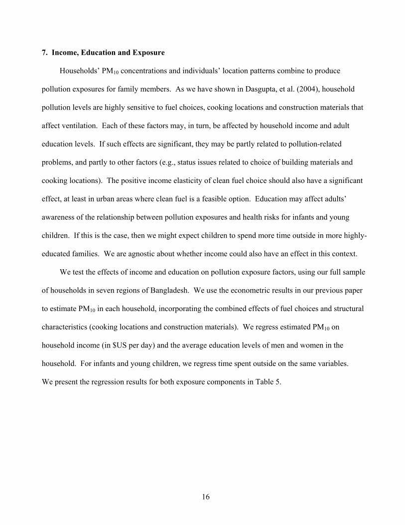
7. Income, Education and Exposure
Households’ PM10 concentrations and individuals’ location patterns combine to produce
pollution exposures for family members. As we have shown in Dasgupta, et al. (2004), household
pollution levels are highly sensitive to fuel choices, cooking locations and construction materials that
affect ventilation. Each of these factors may, in turn, be affected by household income and adult
education levels. If such effects are significant, they may be partly related to pollution-related
problems, and partly to other factors (e.g., status issues related to choice of building materials and
cooking locations). The positive income elasticity of clean fuel choice should also have a significant
effect, at least in urban areas where clean fuel is a feasible option. Education may affect adults’
awareness of the relationship between pollution exposures and health risks for infants and young
children. If this is the case, then we might expect children to spend more time outside in more highly-
educated families. We are agnostic about whether income could also have an effect in this context.
We test the effects of income and education on pollution exposure factors, using our full sample
of households in seven regions of Bangladesh. We use the econometric results in our previous paper
to estimate PM10 in each household, incorporating the combined effects of fuel choices and structural
characteristics (cooking locations and construction materials). We regress estimated PM10 on
household income (in $US per day) and the average education levels of men and women in the
household. For infants and young children, we regress time spent outside on the same variables.
We present the regression results for both exposure components in Table 5.

17
Table 5: Education, Income and Pollution Exposure for Children
(1) (2) (3) Cooking Area Living Area Hours Outside House PM10(ug/m3) PM10(ug/m3) (Children 0-5) Adult Education Level (Range: 0-4) Female -20.305 -14.404 0.130 (7.77)** (7.11)** (0.69) Male -7.556 -6.546 -0.612 (3.36)** (3.76)** (3.85)** Income Per Capita -9.753 -4.752 0.033 ($US Per Day) (4.82)** (3.03)** (0.18) Constant 298.616 252.849 5.145 (87.64)** (95.78)** (21.73)** Observations 4,174 4,174 483 R-squared 0.07 0.06 0.04 Absolute value of t statistics in parentheses * significant at 5%; ** significant at 1%
Education and household per capita income have the expected effects on determinants of indoor
air pollution. All estimated effects are large, highly significant, and have the expected negative sign.
Women’s education has a particularly large effect. Our results indicate that when men’s and women’s
education levels jointly increase from 0 (no primary schooling) to 4 (post-secondary education),
predicted PM10 in the cooking area decreases by about 110 ug/m3. This is a very large effect, since the
average PM10 concentration for our 236 monitored households is 260 ug/m3. Each increase of
$US 1.00/day is associated with a decline of 10 ug/m3, so the predicted reduction over the sample
income range (less than $.50/day to $15.00/day) is approximately 150 ug/m3.
Although education and income strongly reduce average pollution, they do not seem to change
children’s daily activity patterns in ways that reduce pollution exposure. Children’s hours spent
outdoors are not significantly affected by women’s education or income per capita, and the measured

18
effect of adult male education is actually perverse (children of more educated men spend less time
outdoors).
We tentatively conclude that parents’ education and income do affect children’s pollution
exposure, but only through the determinants of pollution. We extend the analysis by estimating
separate regressions for fuel choice and structural determinants of pollution (cooking locations,
construction materials). We combine information on fuel choices and structural characteristics into
two separate indices, with weights determined by the regression coefficients for cooking-area pollution
determinants in Table 7 of Dasgupta, et al. (2004). Table 6 presents the results, which suggest that
female education, male education and family income all have large, highly-significant effects on
pollution via fuel choice. Female education has an equivalent effect on the structural determinants, but
male education and family income do not appear to be significant. As in the composite result (Table
5), female education appears to be the strongest and most pervasive determinant of arrangements that
reduce indoor air pollution.
Table 6: Income, Education and Determinants of Indoor Air Pollution Fuel Construction Materials Choice Cooking Location Adult Education Level (Range: 0-4) Female -8.687 -6.926 (12.00)** (3.85)** Male -7.555 -2.151 (12.14)** (1.39) Income Per Capita -12.760 1.547 ($US Per Day) (22.79)** (1.11) Constant 15.511 22.031 (16.44)** (9.40)** Observations 4,174 4,174 R-squared 0.36 0.01 Absolute value of t statistics in parentheses significant at 5%; ** significant at 1%
19
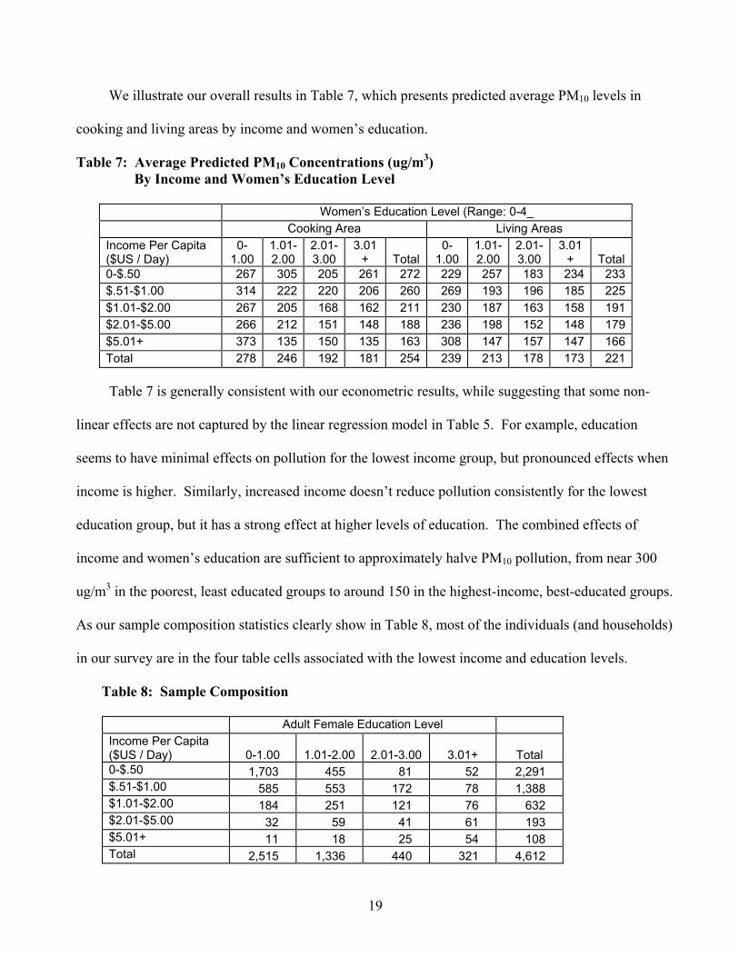
We illustrate our overall results in Table 7, which presents predicted average PM10 levels in
cooking and living areas by income and women’s education.
Table 7: Average Predicted PM10 Concentrations (ug/m3) By Income and Women’s Education Level
Women’s Education Level (Range: 0-4_ Cooking Area Living Areas Income Per Capita ($US / Day)
0-1.00
1.01-2.00
2.01-3.00
3.01+
Total
0-1.00
1.01-2.00
2.01-3.00
3.01+
Total
0-$.50 267 305 205 261 272 229 257 183 234 233$.51-$1.00 314 222 220 206 260 269 193 196 185 225$1.01-$2.00 267 205 168 162 211 230 187 163 158 191$2.01-$5.00 266 212 151 148 188 236 198 152 148 179$5.01+ 373 135 150 135 163 308 147 157 147 166Total 278 246 192 181 254 239 213 178 173 221
Table 7 is generally consistent with our econometric results, while suggesting that some non-
linear effects are not captured by the linear regression model in Table 5. For example, education
seems to have minimal effects on pollution for the lowest income group, but pronounced effects when
income is higher. Similarly, increased income doesn’t reduce pollution consistently for the lowest
education group, but it has a strong effect at higher levels of education. The combined effects of
income and women’s education are sufficient to approximately halve PM10 pollution, from near 300
ug/m3 in the poorest, least educated groups to around 150 in the highest-income, best-educated groups.
As our sample composition statistics clearly show in Table 8, most of the individuals (and households)
in our survey are in the four table cells associated with the lowest income and education levels.
Table 8: Sample Composition
Adult Female Education Level Income Per Capita ($US / Day)
0-1.00
1.01-2.00
2.01-3.00
3.01+
Total
0-$.50 1,703 455 81 52 2,291 $.51-$1.00 585 553 172 78 1,388 $1.01-$2.00 184 251 121 76 632 $2.01-$5.00 32 59 41 61 193 $5.01+ 11 18 25 54 108 Total 2,515 1,336 440 321 4,612

20
8. Summary and Conclusions
In this paper, we have investigated individuals’ exposure to indoor air pollution (IAP) in
Bangladesh. We have analyzed exposure at two levels: differences within households attributable to
family roles, and differences across households attributable to income and education. Within
households, we have related individuals’ exposure to pollution in different locations during their daily
round of activity. We find high levels of exposure for children and adolescents of both sexes, with
particularly serious exposure for children under 5. Among prime-age adults, we find that men have
half the exposure of women (whose exposure is similar to that of children and adolescents). We also
find that elderly men have significantly lower exposure than elderly women.
Across households, we draw on results from our previous paper (Dasgupta, et al., 2004), which
relates pollution variation across households to choices of cooking fuel, cooking locations,
construction materials and ventilation practices. We find that these choices are significantly affected
by family income and adult education levels (particularly for women). Overall, we find that the
poorest, least-educated households have twice the pollution levels of relatively high-income
households with highly-educated adults.
To summarize, we find that young children and poorly-educated women in poor households face
pollution exposures that are four times those of men in higher-income households organized by more
highly-educated women. In our previous paper, we recommended feasible changes in cooking
locations, construction materials and ventilation practices that could greatly reduce average household
pollution levels. In this paper, we consider measures for narrowing the exposure gap within
households. We focus particularly on changes for infants and young children, since they suffer the
worst mortality and morbidity from indoor air pollution, but our findings also apply to women and
adolescents. Our recommendations for reducing their exposure are based on a few simple, robust

21
findings: Hourly pollution levels in cooking and living areas are quite similar because cooking smoke
diffuses rapidly and nearly-completely into living areas. At the same time, outdoor pollution is far
lower. At present, young children are only outside for an average of 3 hours per day. For children in a
typical household, pollution exposure can be halved by adopting two simple measures: increasing
their outdoor time from 3 to 5 or 6 hours per day, and concentrating outdoor time during peak cooking
periods. We recognize that weather and other factors may intervene occasionally, and that child
supervision outdoors may be difficult for some households. However, the potential benefits are so
great that neighbors might well agree to pool outdoor supervision once they became aware of the
implications for their children’s health.

22
References
Bruce, N., 1999, Lowering Exposure of Children to Indoor Air Pollution to Prevent ARI: the Need for Information and Action, Capsule Report (3), Environmental Health Project, Arlington VA. Dasgupta, S., M. Huq., M. Khaliquzzaman, K. Pandey, and D.Wheeler, 2004, “Indoor Air Quality for Poor Families: New Evidence from Bangladesh,” World Bank, Development Research Group Working Paper No. 3393, August. Galassi, C., B. Ostro, F. Forastiere, S. Cattani, M. Martuzzi and R. Bertollini, 2000, “Exposure to PM10 in the Eight Major Italian Cities and Quantification of the Health Effects,” presented to ISEE 2000, Buffalo, New York, August 19-22. Kirkwood, B., S. Gove, S. Rogers, J. Lob-Levyt, P. Arthur and H. Campbell, 1995, "Potential Interventions for the Prevention of Childhood Pneumonia in Developing Countries: A Systematic Review,” Bulletin of the World Health Organization, 73: 793-798. Murray, C. and A. Lopez (eds.), 1996, The Global Burden of Disease, Cambridge MA: Harvard School of Public Health, WHO, World Bank. Smith, K., 2000, “National Burden of Disease in India From Indoor Air Pollution,” Proceedings of the National Academy of Science USA, (97) 13286-13293. Smith, K. and S. Metha, 2000, The Global Burden of Disease from Indoor Air Pollution in Developing Countries: Comparison of Estimates, Prepared for the WHO/USAID Global Technical Consultation on Health Impacts of Indoor Air Pollution in Developing Countries. Smith, K., 1993, “Fuel Combustion, Air Pollution Exposure, and Health: the Situation in Developing Countries," Annual Review of Environment and Energy, 18:526-566. Smith, K., Y, Liu, J. Rivera, et al., 1993. “Indoor air quality and child exposures in highland Guatemala,” Proceedings of the 6th International Conference on Indoor Air Quality and Climate, University of Technology, Helsinki, 1:441-446. Von Schrinding, Y., N. Bruce, K. Smith, G. Ballars-Treemeer, M. Errati, and K. Lvovsky, 2001, Addressing the Impact of Household Energy and Indoor Air Pollution on the Health of the Poor—Implications for Policy Action and Intervention Measures, WHO Commission on Macroeconomics and Health Working Paper, WG5:12. WHO, 2001, Informal Consultation on Epidemiologic Estimates for Child Health 11-12 June 2001, Department of Child and Adolescent Health Development, WHO, Geneva (http://www.who.int/child-adolescent-health/New Publications/Overview/). World Bank, 2002, “India: Household Energy, Indoor Air Pollution, and Health,” ESMAP / South Asia Environment and Social Development Unit, November.
23
World Bank, 2001, Making Sustainable Commitments: An Environment Strategy for the World Bank, July.

Appendix I: Hourly Household Member Locations, by Age and Gender (X = Presence in a Location)
Time (0 = 12:00 AM; 23 = 11:00 PM) Sex Age Place 0 1 2 3 4 5 6 7 8 9 10 11 12 13 14 15 16 17 18 19 20 21 22 23 Total
F 0-1 K X 1 F 0-1 L X X X X X X X X X X X X X X X X X X X X 22 F 0-1 O X X X 1 F 1-5 K X 1 F 1-5 L X X X X X X X X X X X X X X X X X X X 19 F 1-5 O X X X X 4 F 6-8 K X 1 F 6-8 L X X X X X X X X X X X X X X X X X 17 F 6-8 O X X X X X X 6 F 9-18 K X X 2 F 9-18 L X X X X X X X X X X X X X X X X 16 F 9-18 O X X X X X X 6 F 19-60 K X X X X 4 F 19-60 L X X X X X X X X X X X X X X X X X X 18 F 19-60 O X X 2 F 60+ K X X 2 F 60+ L X X X X X X X X X X X X X X X X X X X 19 F 60+ O X X X 3 M 0-1 K X 1 M 0-1 L X X X X X X X X X X X X X X X X X X X X 20 M 0-1 O X X X 3 M 1-5 K X 1 M 1-5 L X X X X X X X X X X X X X X X X X X X 19 M 1-5 O X X X X 4 M 6-8 K X 1 M 6-8 L X X X X X X X X X X X X X X X X 16 M 6-8 O X X X X X X X 7 M 9-18 K 0 M 9-18 L X X X X X X X X X X X X X X X X 16 M 9-18 O X X X X X X X X 8 M 19-60 K 0 M 19-60 L X X X X X X X X X X X X X 13 M 19-60 O X X X X X X X X X X X 11 M 60+ K 0 M 60+ L X X X X X X X X X X X X X X X X 16 M 60+ O X X X X X X X X 8