whitepaper at SIGGRAPH 2015 - DEPARTMENT OF …ari/Publications/SIGGRAPH...2015-08-24 · whitepaper...
164
Multi-Scale Global Illumination in Quantum Break Ari Silvennoinen Ville Timonen Remedy Entertainment Aalto University Remedy Entertainment SIGGRAPH 2015: Advances in Real-Time Rendering course
Transcript of whitepaper at SIGGRAPH 2015 - DEPARTMENT OF …ari/Publications/SIGGRAPH...2015-08-24 · whitepaper...
Multi-Scale Global Illumination in Quantum Break
Ari Silvennoinen Ville TimonenRemedy Entertainment
Aalto UniversityRemedy Entertainment
SIGGRAPH 2015: Advances in Real-Time Rendering course
Remedy Entertainment
SIGGRAPH 2015: Advances in Real-Time Rendering course
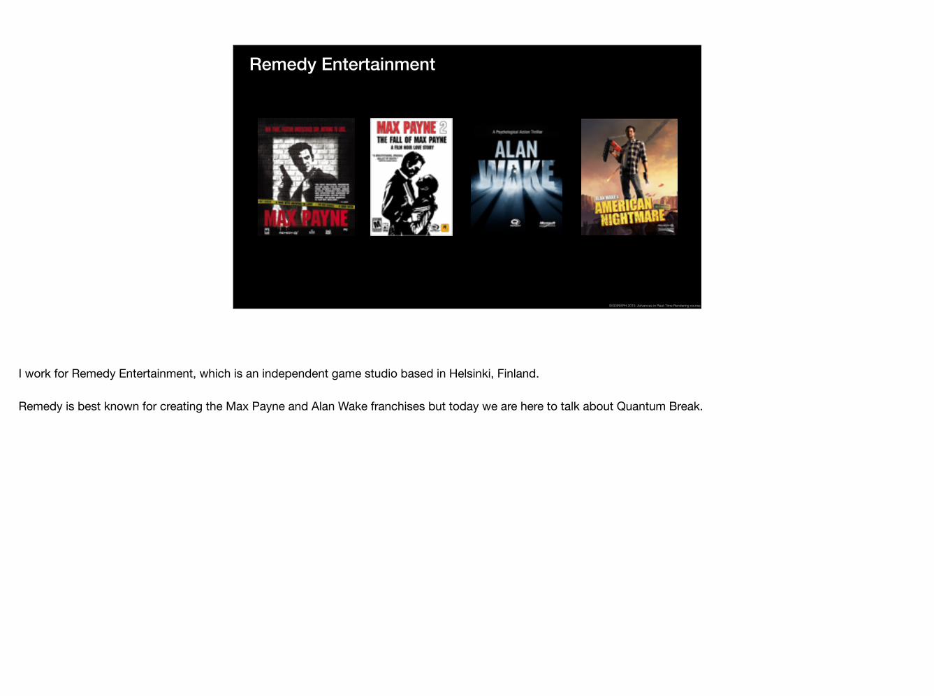
I work for Remedy Entertainment, which is an independent game studio based in Helsinki, Finland.
Remedy is best known for creating the Max Payne and Alan Wake franchises but today we are here to talk about Quantum Break.

Before we go any further, let’s take a look at a video to find out what the game is all about.
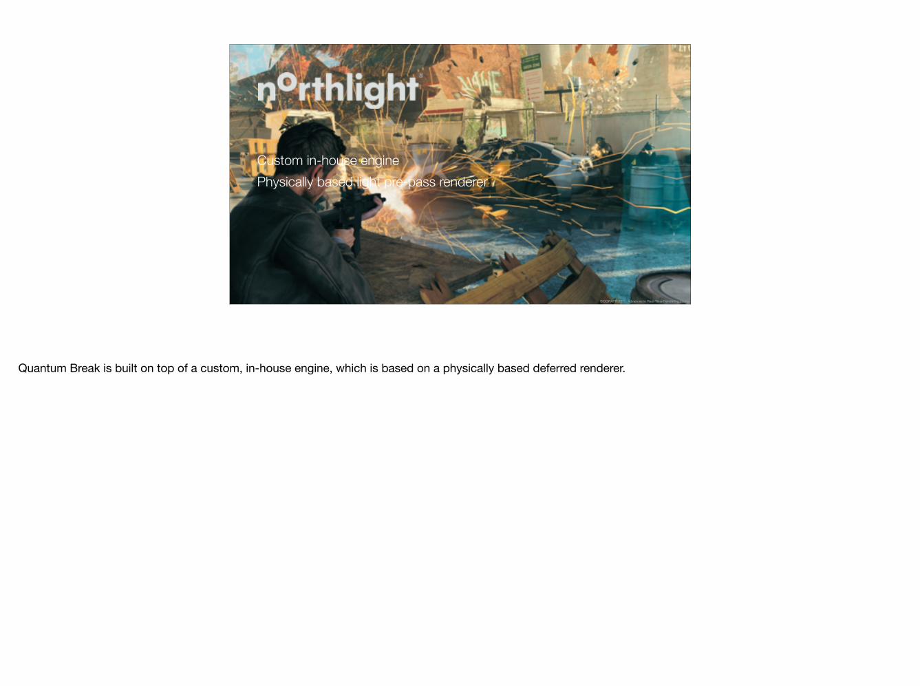
Custom in-house engine Physically based light pre-pass renderer
SIGGRAPH 2015: Advances in Real-Time Rendering course
Quantum Break is built on top of a custom, in-house engine, which is based on a physically based deferred renderer.
SIGGRAPH 2015: Advances in Real-Time Rendering course
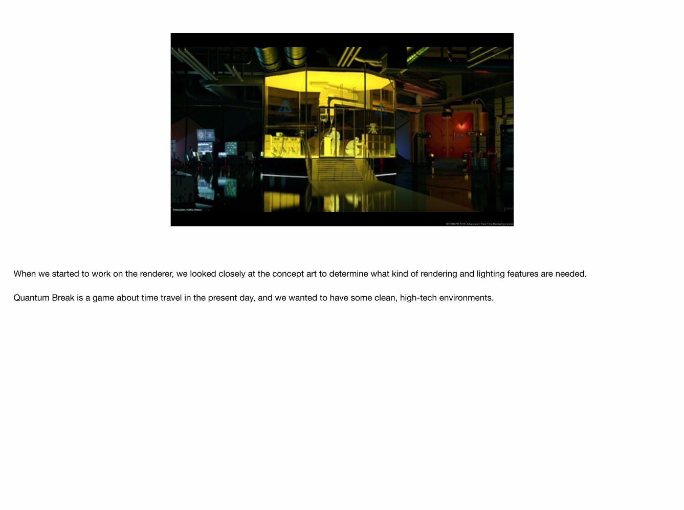
When we started to work on the renderer, we looked closely at the concept art to determine what kind of rendering and lighting features are needed.
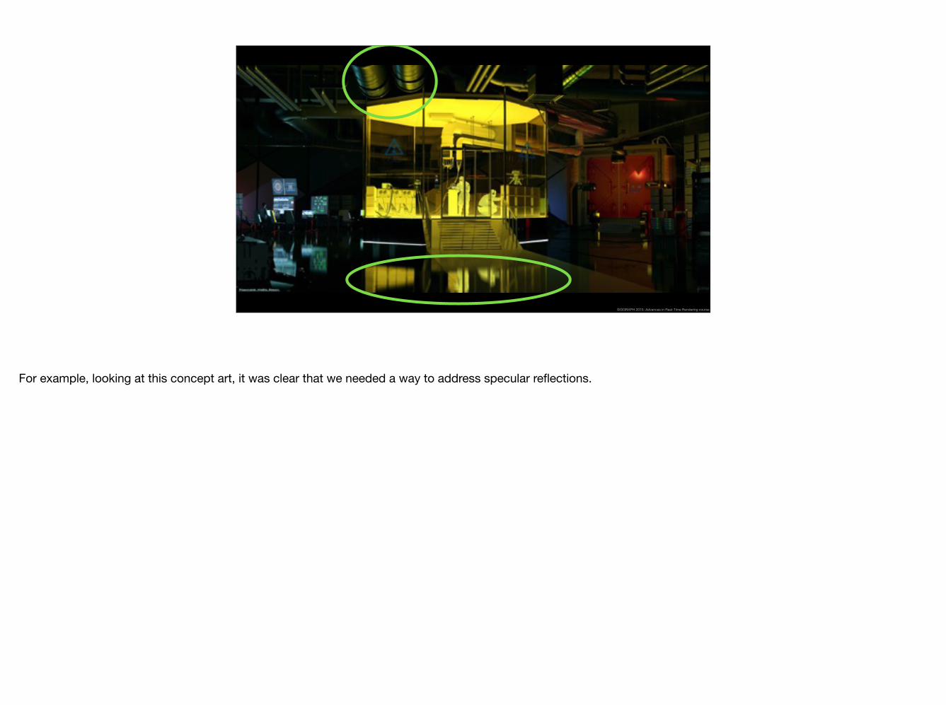
Quantum Break is a game about time travel in the present day, and we wanted to have some clean, high-tech environments.
SIGGRAPH 2015: Advances in Real-Time Rendering course
For example, looking at this concept art, it was clear that we needed a way to address specular reflections.
SIGGRAPH 2015: Advances in Real-Time Rendering course
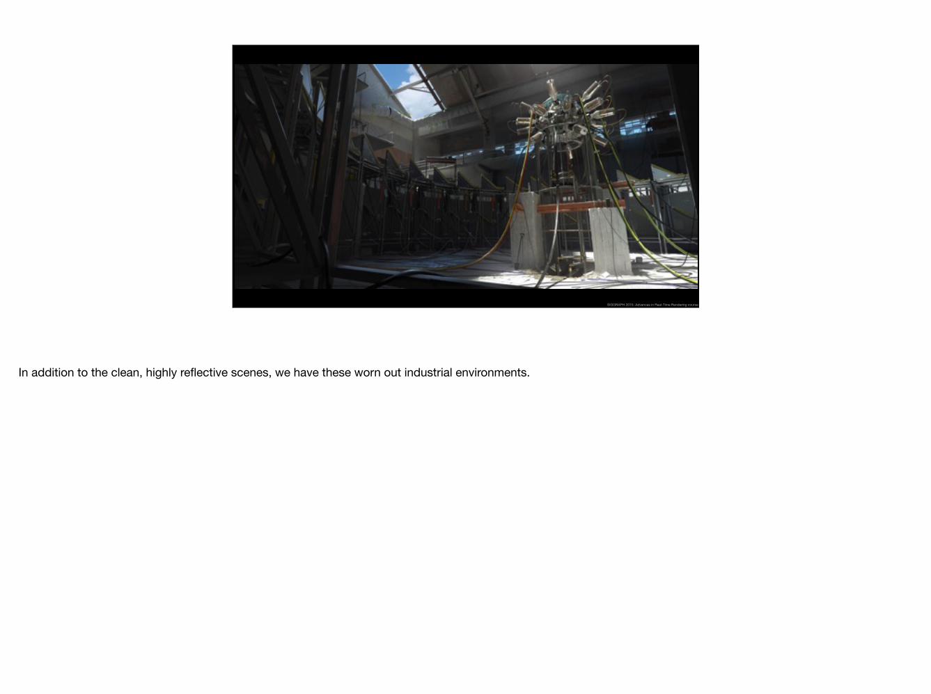
In addition to the clean, highly reflective scenes, we have these worn out industrial environments.
SIGGRAPH 2015: Advances in Real-Time Rendering course
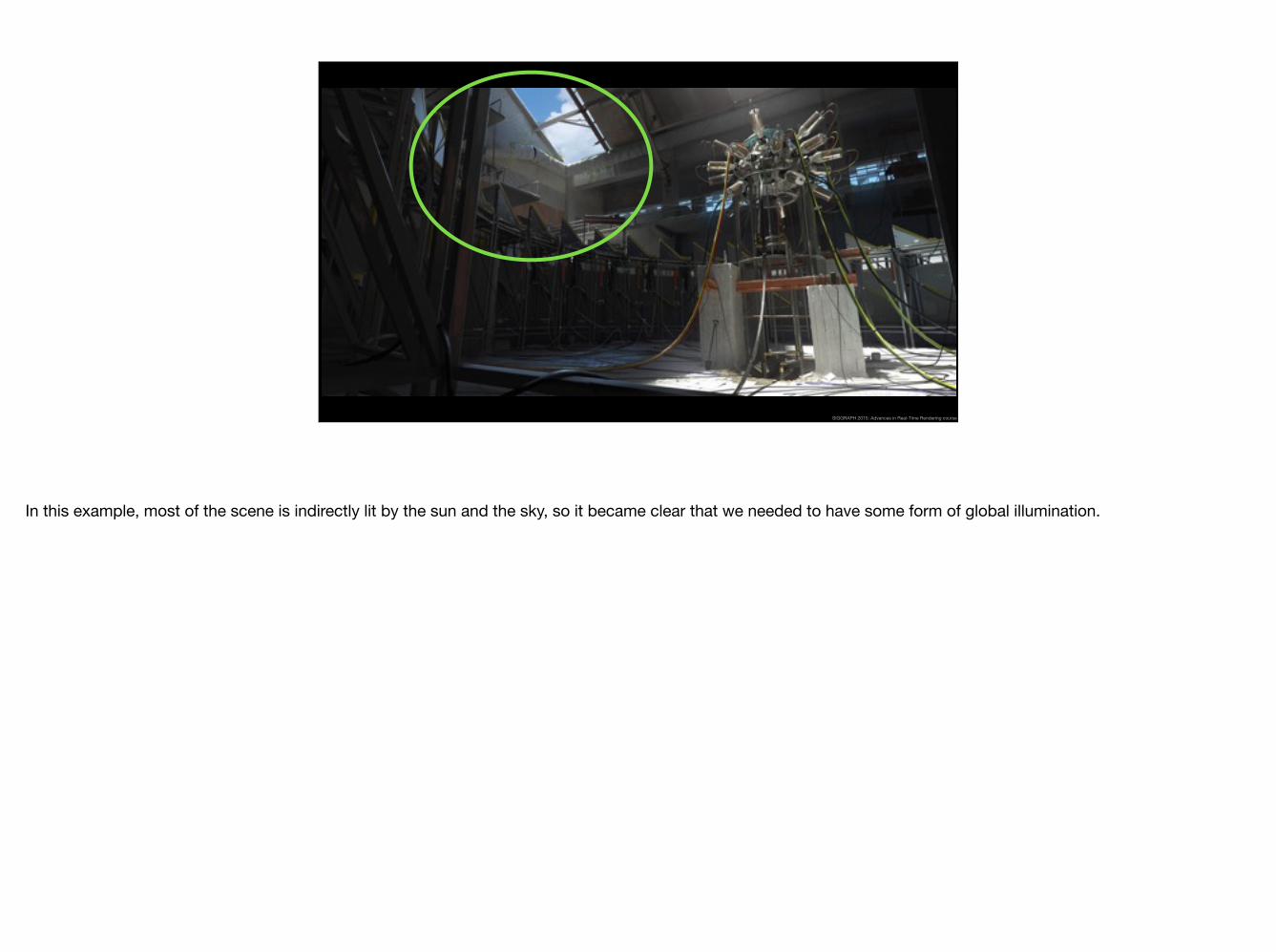
In this example, most of the scene is indirectly lit by the sun and the sky, so it became clear that we needed to have some form of global illumination.
SIGGRAPH 2015: Advances in Real-Time Rendering course
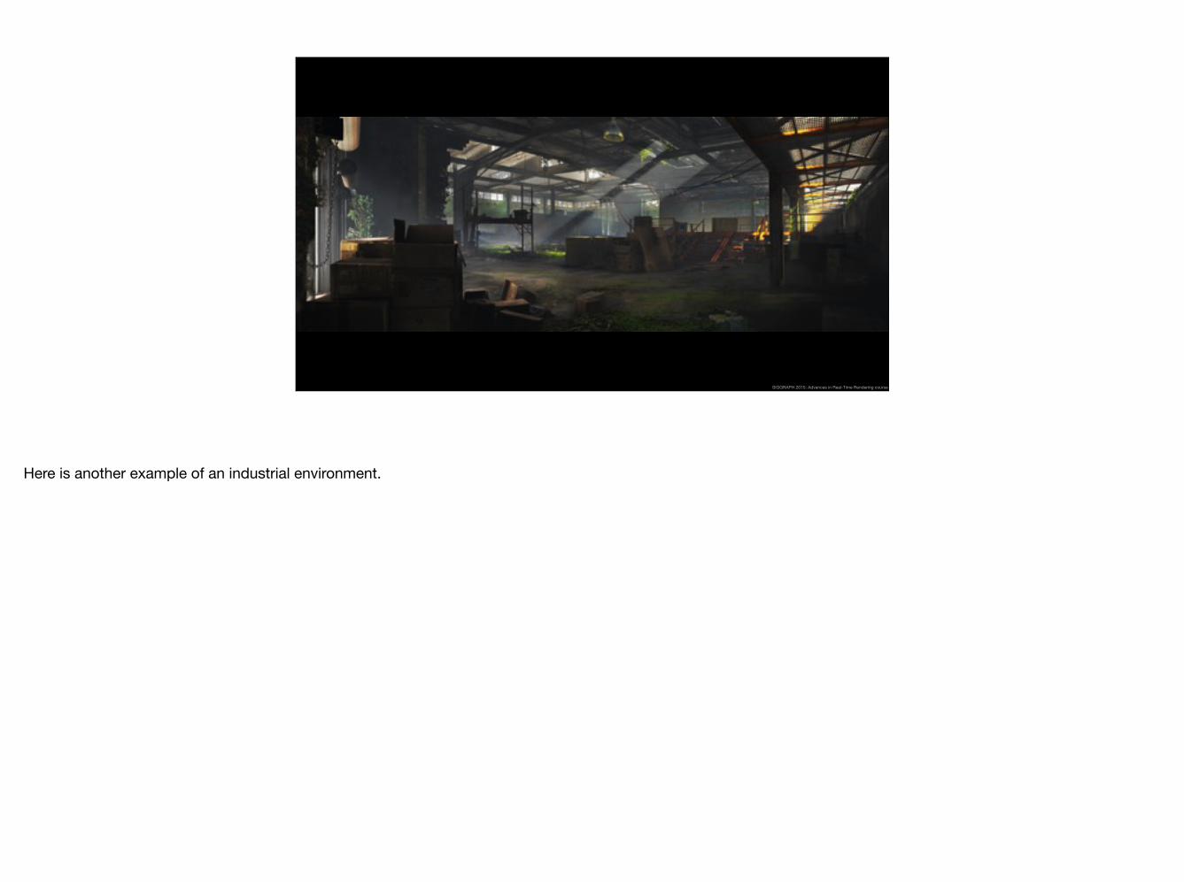
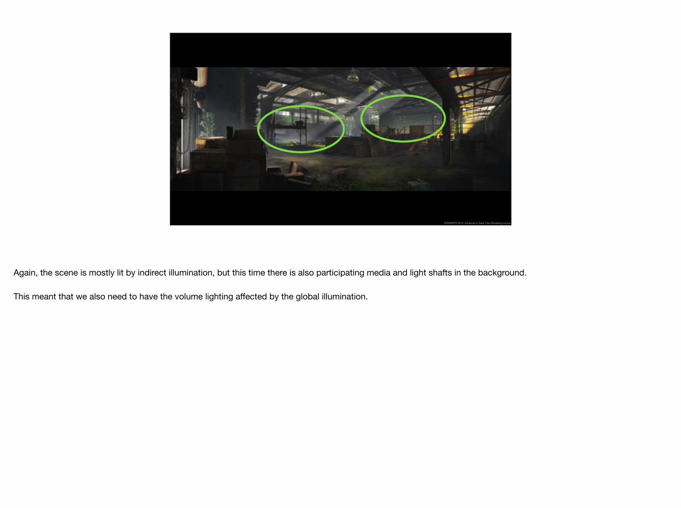
Here is another example of an industrial environment.
SIGGRAPH 2015: Advances in Real-Time Rendering course
Again, the scene is mostly lit by indirect illumination, but this time there is also participating media and light shafts in the background.
This meant that we also need to have the volume lighting affected by the global illumination.

Design Goals and Constraints
Consistency
SIGGRAPH 2015: Advances in Real-Time Rendering course
One of our primary goals with the new renderer was consistency across the lighting.
We wanted to have the environments, dynamic objects, particles and volumetric lights all blend in together seamlessly.

Design Goals and Constraints
Consistency Semi-dynamic environments and lighting
SIGGRAPH 2015: Advances in Real-Time Rendering course
The second constraint was that we had to support large scale destruction events and, in some levels, dynamic time of day.

Design Goals and Constraints
Consistency Semi-dynamic environments and lighting Fully automatic
SIGGRAPH 2015: Advances in Real-Time Rendering course
Finally, since we are a small team, we wanted to have a fully automatic system, which would require minimal amount of artist work.
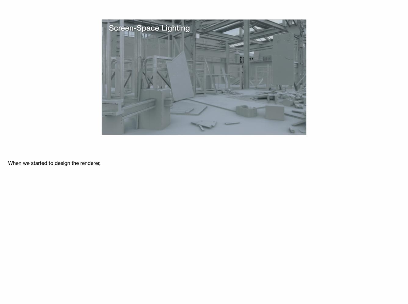
Screen-Space Lighting
SIGGRAPH 2015: Advances in Real-Time Rendering course
When we started to design the renderer,
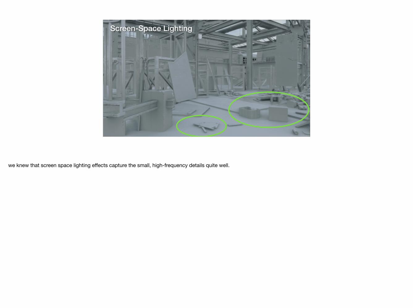
Screen-Space Lighting
SIGGRAPH 2015: Advances in Real-Time Rendering course
we knew that screen space lighting effects capture the small, high-frequency details quite well.
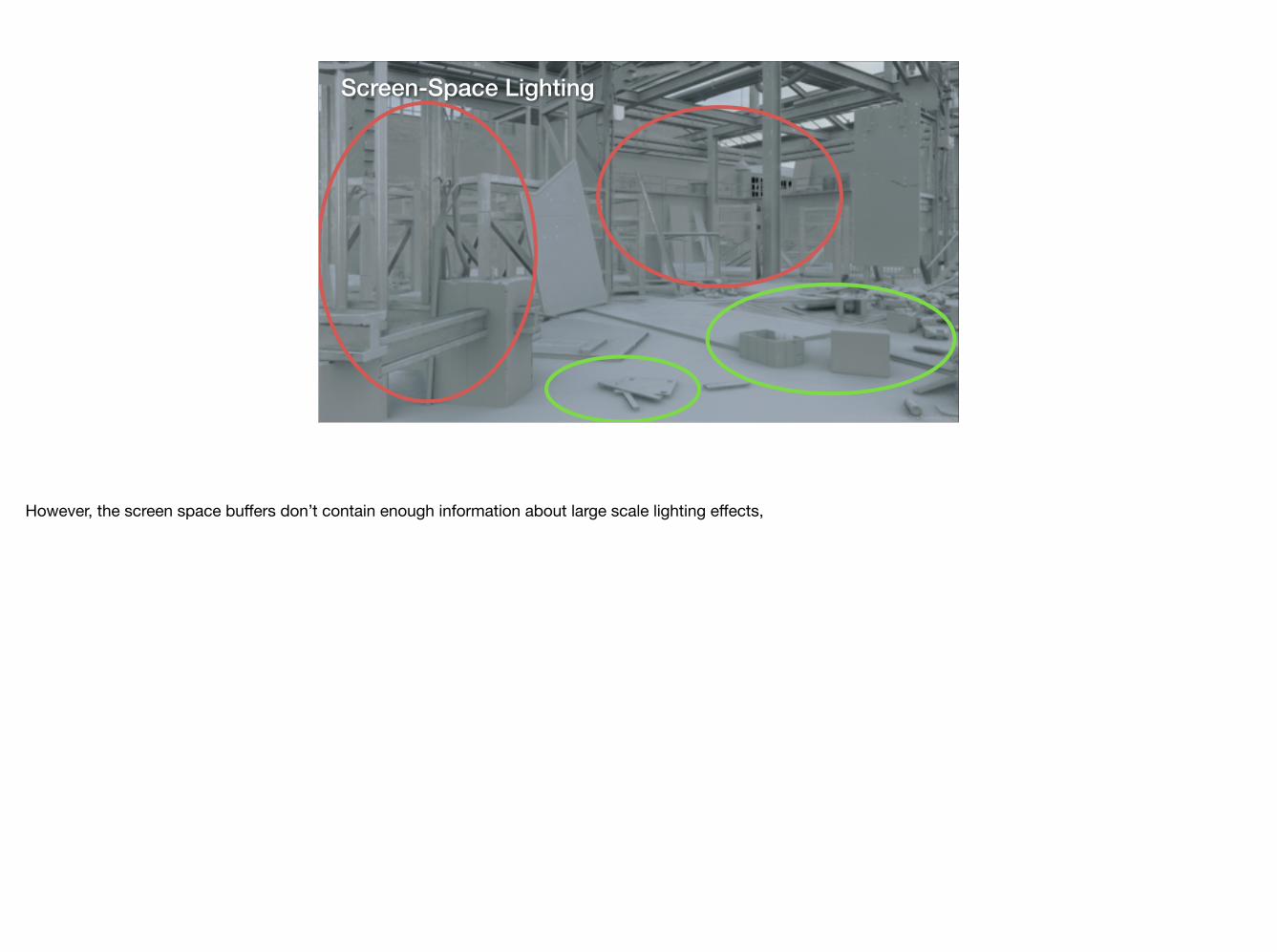
Screen-Space Lighting
SIGGRAPH 2015: Advances in Real-Time Rendering course
However, the screen space buffers don’t contain enough information about large scale lighting effects,
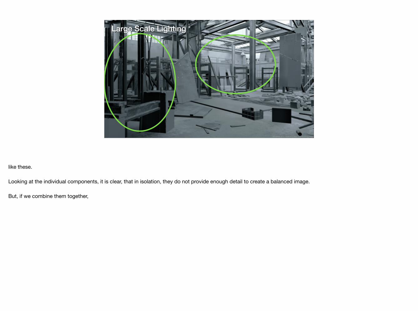
Large Scale Lighting
SIGGRAPH 2015: Advances in Real-Time Rendering course
like these.
Looking at the individual components, it is clear, that in isolation, they do not provide enough detail to create a balanced image.
But, if we combine them together,
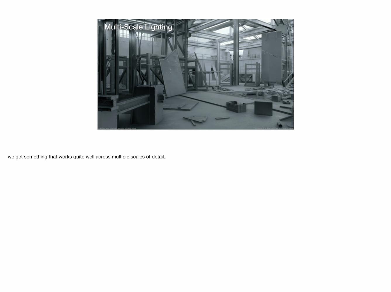
Multi-Scale Lighting
SIGGRAPH 2015: Advances in Real-Time Rendering course SIGGRAPH 2015: Advances in Real-Time Rendering course
we get something that works quite well across multiple scales of detail.

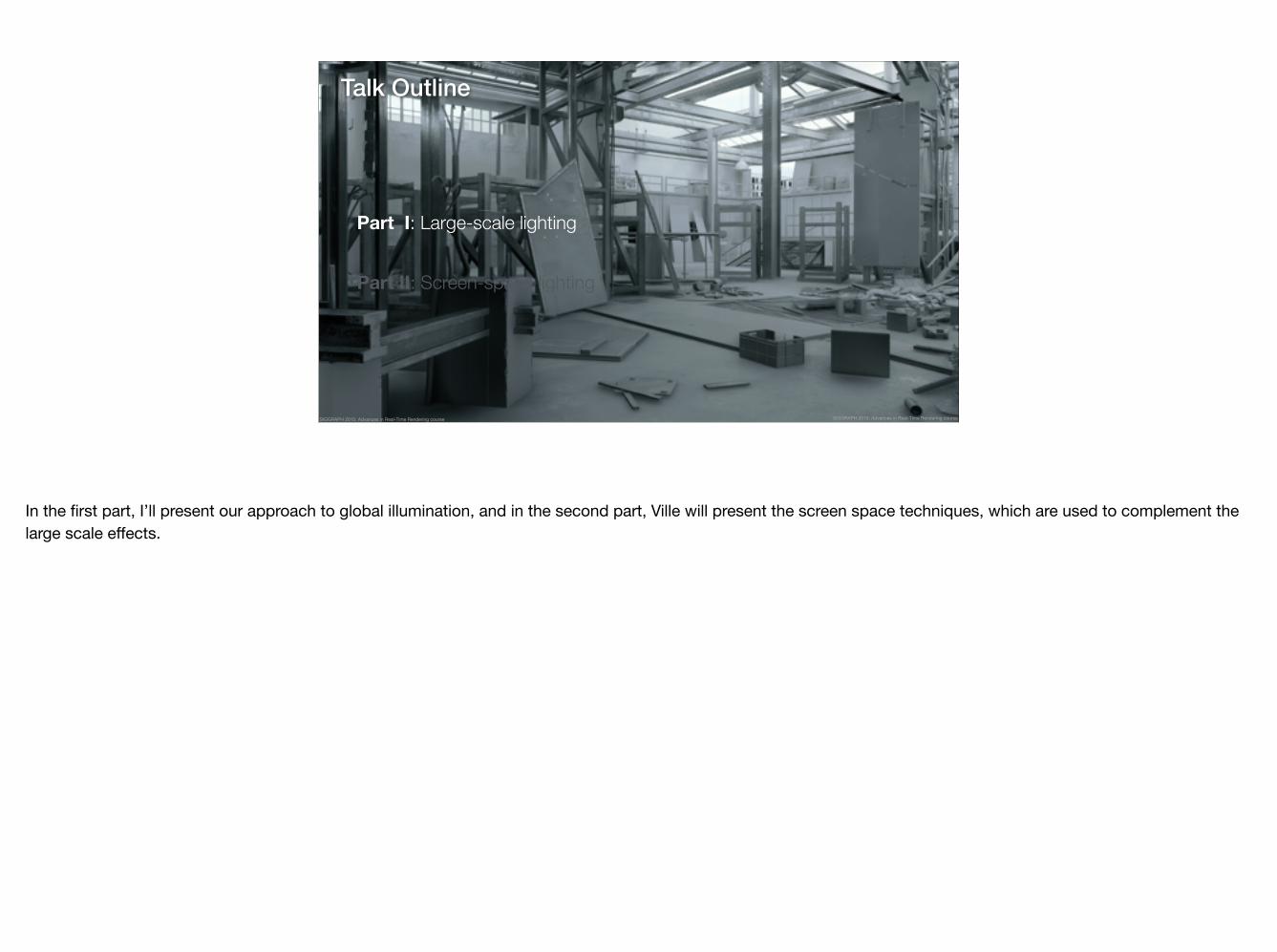
Talk Outline
Part I: Large-scale lighting
Part II: Screen-space lighting
SIGGRAPH 2015: Advances in Real-Time Rendering course SIGGRAPH 2015: Advances in Real-Time Rendering course
So, inspired by this multiscale approach, the rest of the talk is divided into two parts.
Talk Outline
Part I: Large-scale lighting
Part II: Screen-space lighting
SIGGRAPH 2015: Advances in Real-Time Rendering course SIGGRAPH 2015: Advances in Real-Time Rendering course
In the first part, I’ll present our approach to global illumination, and in the second part, Ville will present the screen space techniques, which are used to complement the large scale effects.

Possible Solutions for Global Illumination
Most traditional rendering algorithms fire rays through each pixel —path tracing, etc. —determine intensity by averaging many samples (MC sampling) —sample all possible paths light can take from source to sensor
Not useful for finding derivatives
Dynamic Approaches — Virtual Point Lights (VPLs) [Keller97] — Light Propagation Volumes [Kaplaynan10] — Voxel Cone Tracing [Crassin11] — Distance Field Tracing [Wright15]
SIGGRAPH 2015: Advances in Real-Time Rendering course
Let’s begin with global illumination.
Ideally, the solution would be fully dynamic, and, for every frame, we could compute the global illumination from scratch.

Dynamic Approaches — Virtual Point Lights (VPLs) [Keller97] — Light Propagation Volumes [Kaplaynan10] — Voxel Cone Tracing [Crassin11] — Distance Field Tracing [Wright15]
Cost was too high for the quality we wanted
Possible Solutions for Global Illumination
SIGGRAPH 2015: Advances in Real-Time Rendering course
We experimented with voxel cone tracing and virtual point lights but it became clear that achieving the level of quality we wanted was too expensive with these techniques.

Most traditional rendering algorithms fire rays through each pixel —path tracing, etc. —determine intensity by averaging many samples (MC sampling) —sample all possible paths light can take from source to sensor
Not useful for finding derivatives
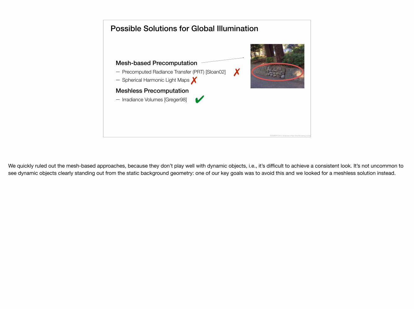
Mesh-based Precomputation — Precomputed Radiance Transfer (PRT) [Sloan02] — Spherical Harmonic Light Maps
Possible Solutions for Global Illumination
Meshless Precomputation — Irradiance Volumes [Greger98]
SIGGRAPH 2015: Advances in Real-Time Rendering course
So, during pre-production, it became clear that we needed to use some form of precomputation.
Most traditional rendering algorithms fire rays through each pixel —path tracing, etc. —determine intensity by averaging many samples (MC sampling) —sample all possible paths light can take from source to sensor
Not useful for finding derivatives
Mesh-based Precomputation — Precomputed Radiance Transfer (PRT) [Sloan02] — Spherical Harmonic Light Maps
Possible Solutions for Global Illumination
Meshless Precomputation — Irradiance Volumes [Greger98]
✗✗
✔
SIGGRAPH 2015: Advances in Real-Time Rendering course
We quickly ruled out the mesh-based approaches, because they don’t play well with dynamic objects, i.e., it’s difficult to achieve a consistent look. It’s not uncommon to see dynamic objects clearly standing out from the static background geometry: one of our key goals was to avoid this and we looked for a meshless solution instead.
Irradiance Volumes
[Greger 1998]SIGGRAPH 2015: Advances in Real-Time Rendering course
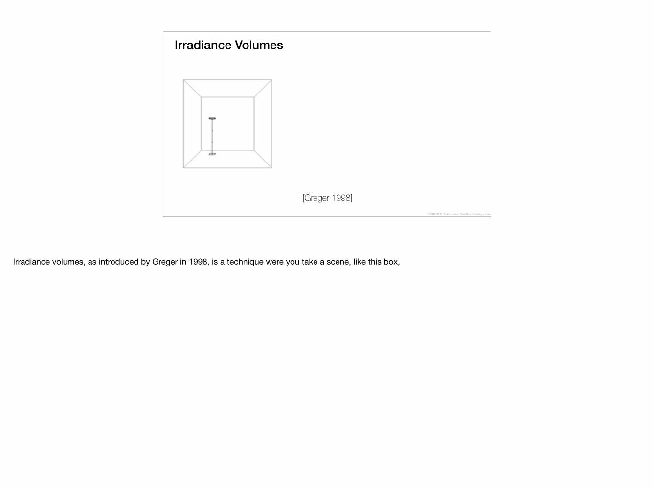
Irradiance volumes, as introduced by Greger in 1998, is a technique were you take a scene, like this box,
Irradiance Volumes
[Greger 1998]SIGGRAPH 2015: Advances in Real-Time Rendering course
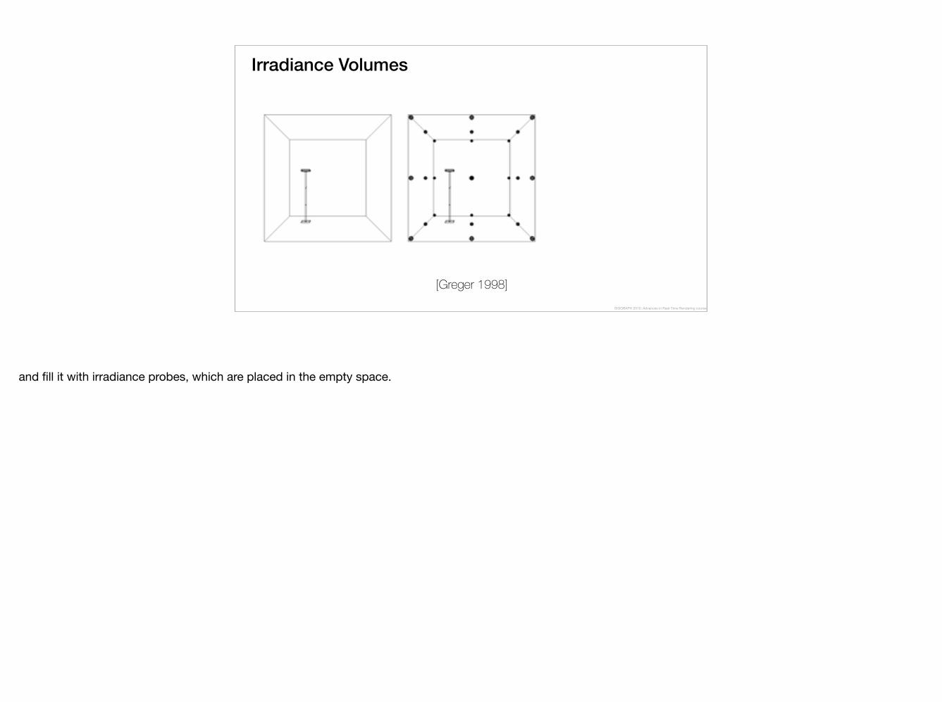
and fill it with irradiance probes, which are placed in the empty space.
Irradiance Volumes
[Greger 1998]SIGGRAPH 2015: Advances in Real-Time Rendering course
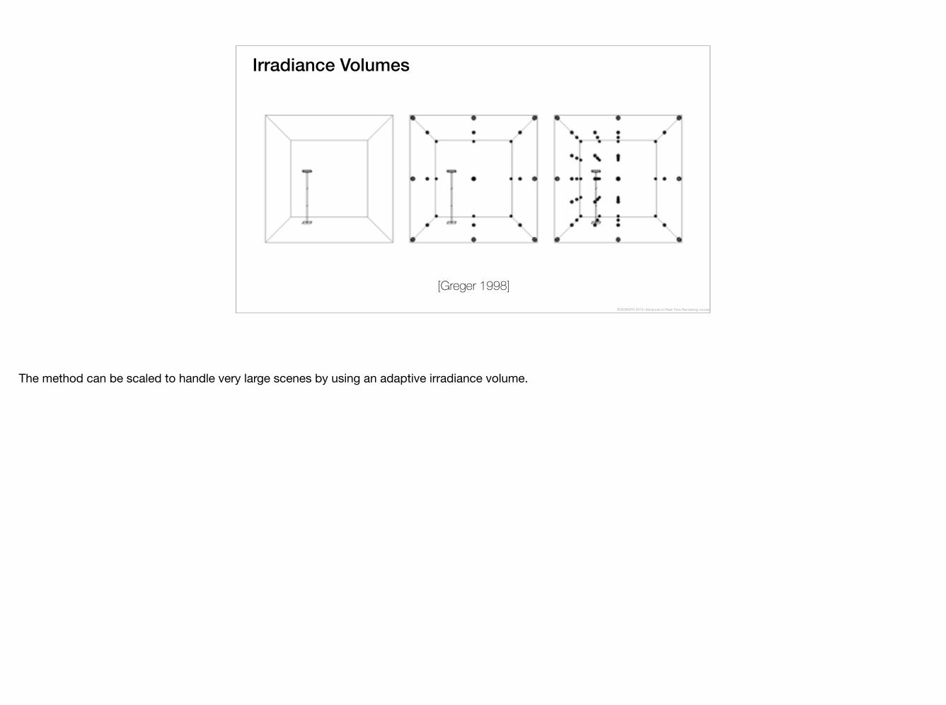
The method can be scaled to handle very large scenes by using an adaptive irradiance volume.
Irradiance Volumes
[Greger 1998]
Per-pixel lookup
SIGGRAPH 2015: Advances in Real-Time Rendering course
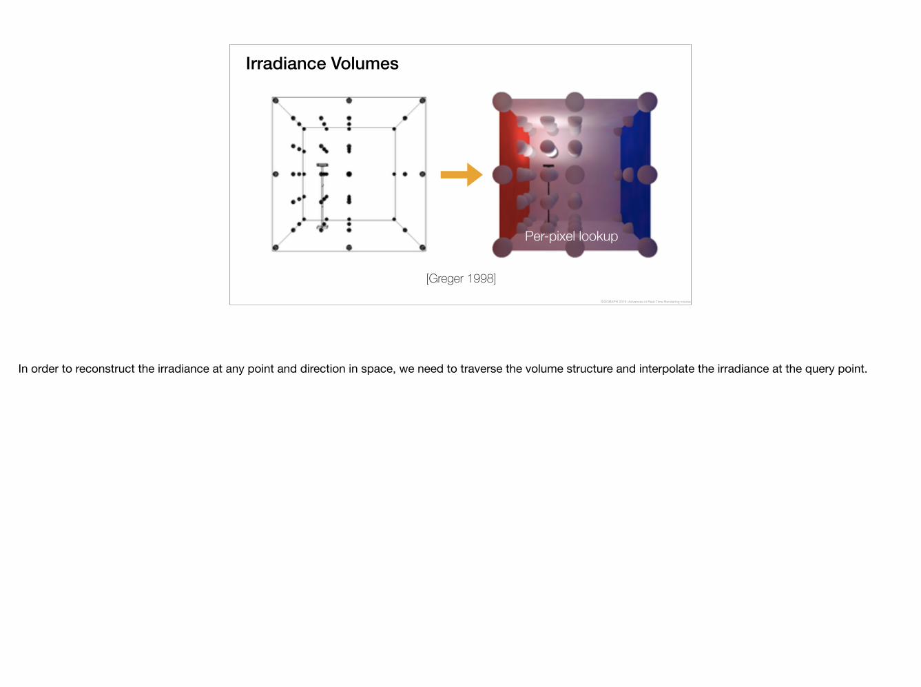
In order to reconstruct the irradiance at any point and direction in space, we need to traverse the volume structure and interpolate the irradiance at the query point.
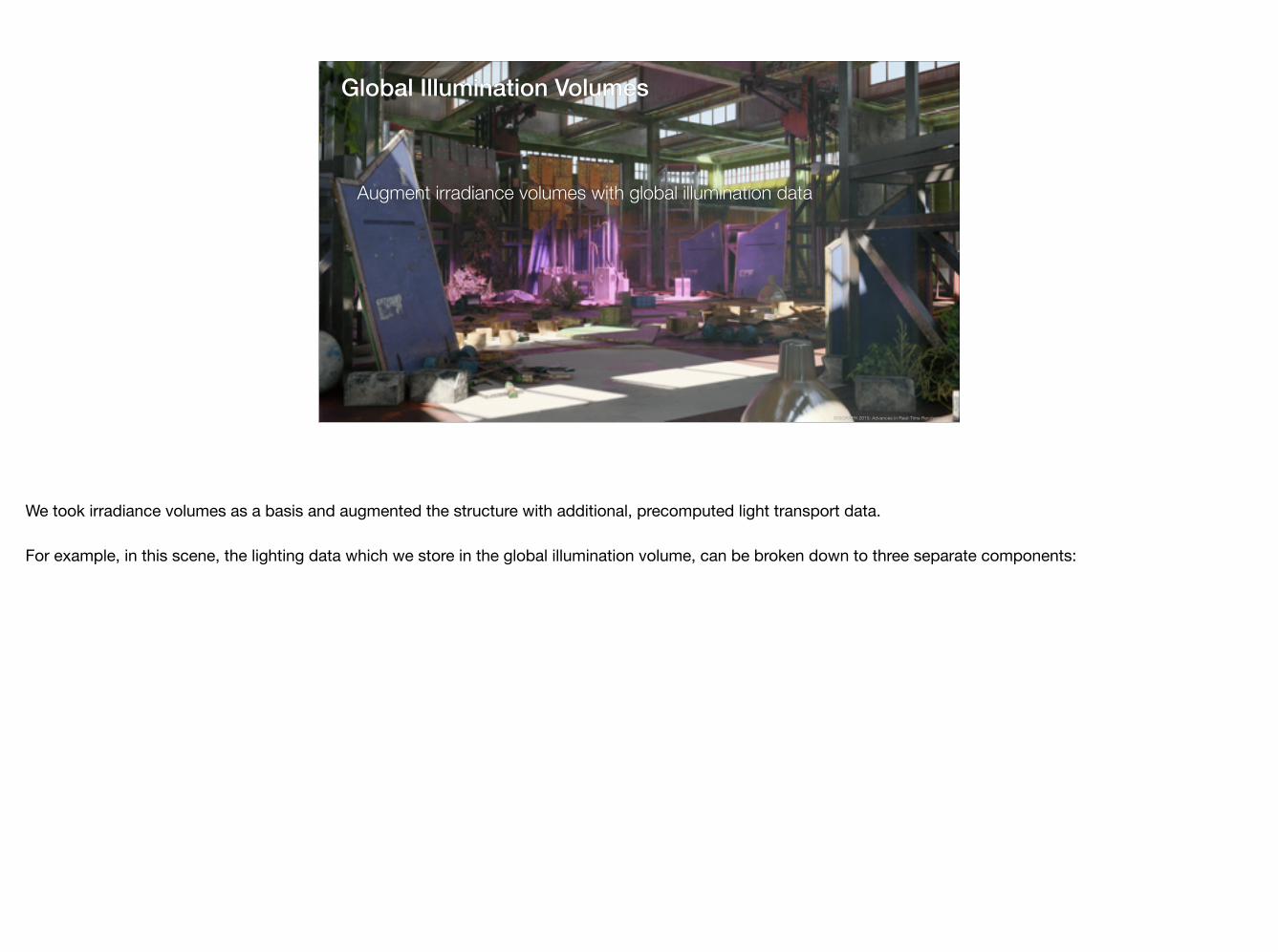
Global Illumination Volumes
Augment irradiance volumes with global illumination data
SIGGRAPH 2015: Advances in Real-Time Rendering course
We took irradiance volumes as a basis and augmented the structure with additional, precomputed light transport data.
For example, in this scene, the lighting data which we store in the global illumination volume, can be broken down to three separate components:
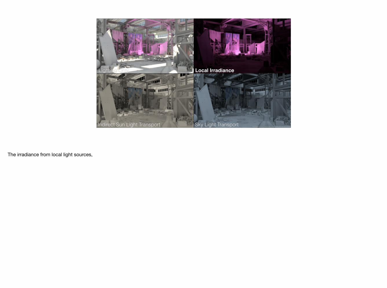
Lighting Only Local Irradiance
Indirect Sun Light Transport Sky Light Transport SIGGRAPH 2015: Advances in Real-Time Rendering course
The irradiance from local light sources,

Lighting Only
Indirect Sun Light Transport Sky Light Transport
Local Irradiance
SIGGRAPH 2015: Advances in Real-Time Rendering course
indirect sun light transport,

Local Irradiance
Indirect Sun Light Transport Sky Light Transport
Lighting Only
SIGGRAPH 2015: Advances in Real-Time Rendering course
and sky light transport.
Local Irradiance
Indirect Sun Light Transport
Lighting Only
Sky Light Transport SIGGRAPH 2015: Advances in Real-Time Rendering course
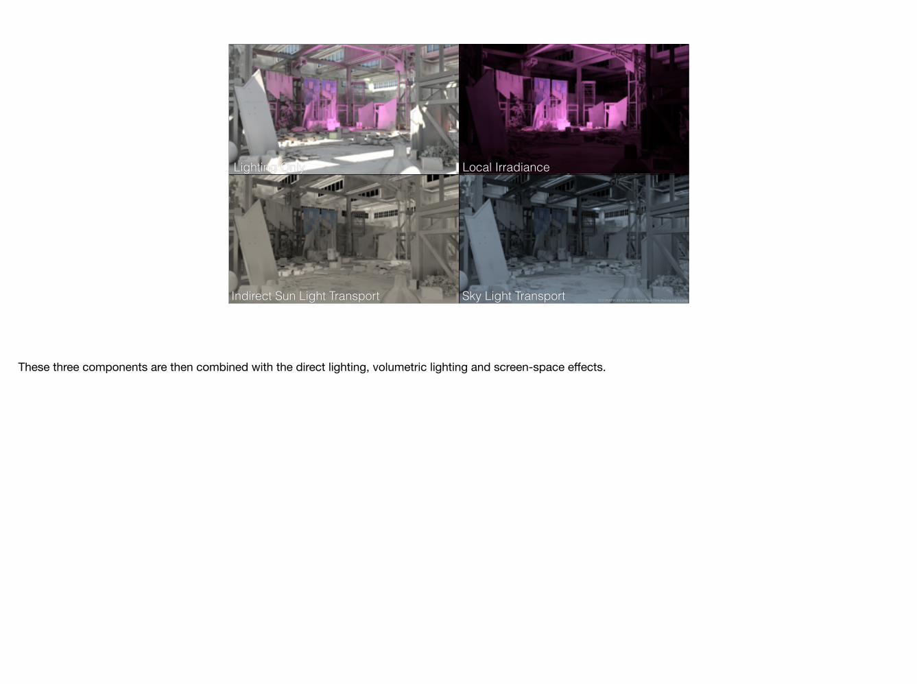
These three components are then combined with the direct lighting, volumetric lighting and screen-space effects.
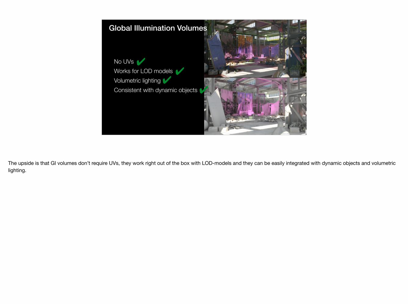
No UVs Works for LOD models Volumetric lighting Consistent with dynamic objects
✔✔
✔
Global Illumination Volumes
✔
SIGGRAPH 2015: Advances in Real-Time Rendering course
The upside is that GI volumes don’t require UVs, they work right out of the box with LOD-models and they can be easily integrated with dynamic objects and volumetric lighting.

No UVs Works for LOD models Volumetric lighting Consistent with dynamic objects
Specular infeasible due to data size
✔✔
✗
✔
Global Illumination Volumes
✔
SIGGRAPH 2015: Advances in Real-Time Rendering course
The only downside is that specular PRT is not really feasible, because having a decent angular resolution would require too much data.
Next, I’ll talk about how we handle specular reflections.
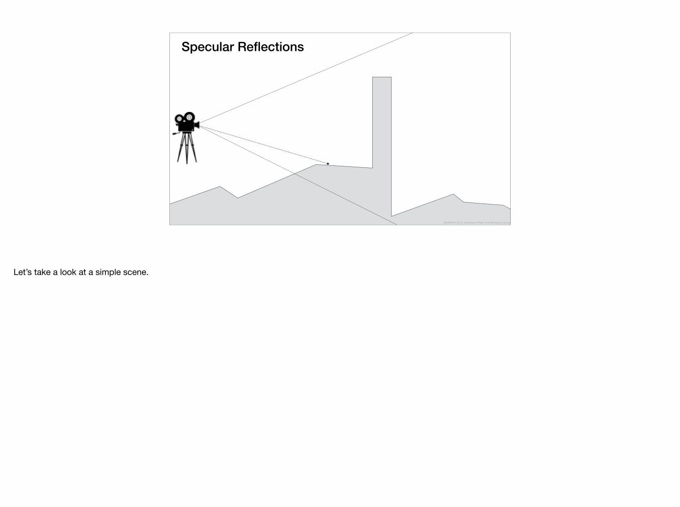
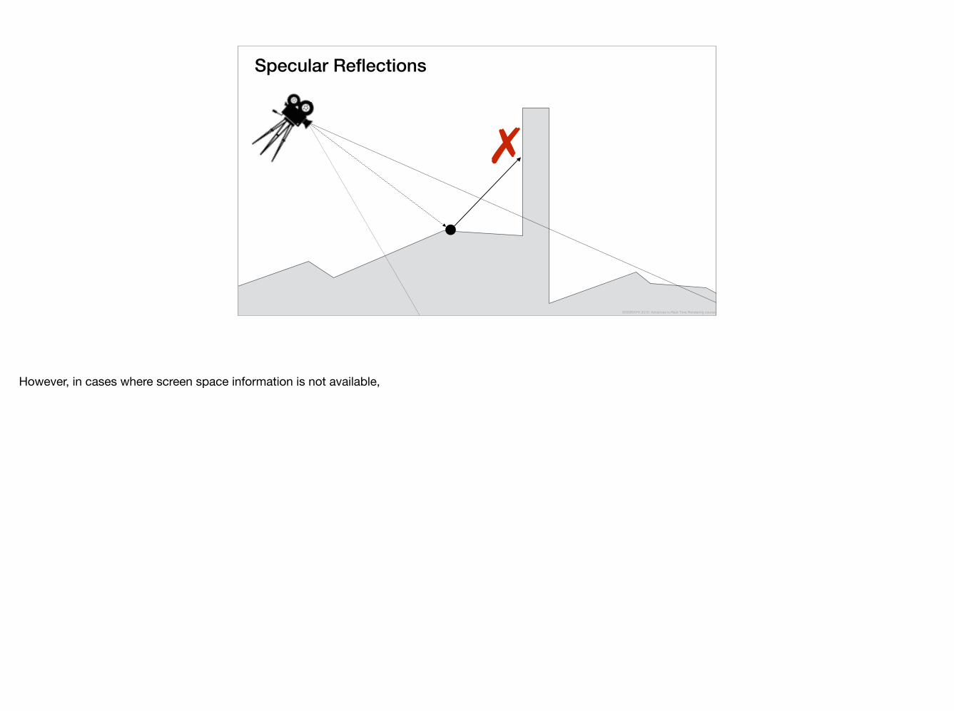
Specular Reflections
SIGGRAPH 2015: Advances in Real-Time Rendering course
Let’s take a look at a simple scene.
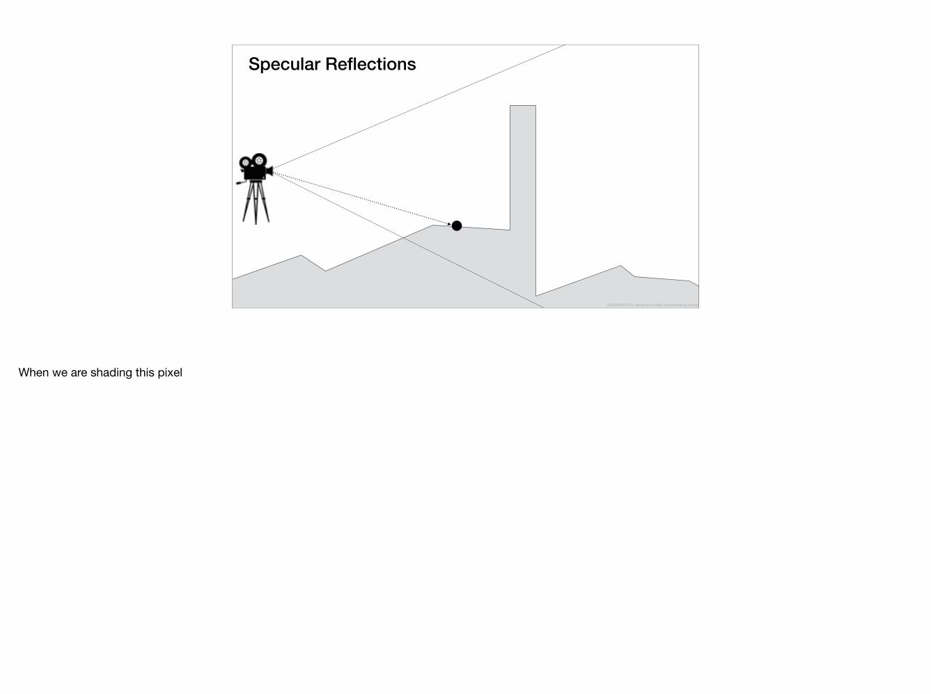
Specular Reflections
SIGGRAPH 2015: Advances in Real-Time Rendering course
When we are shading this pixel
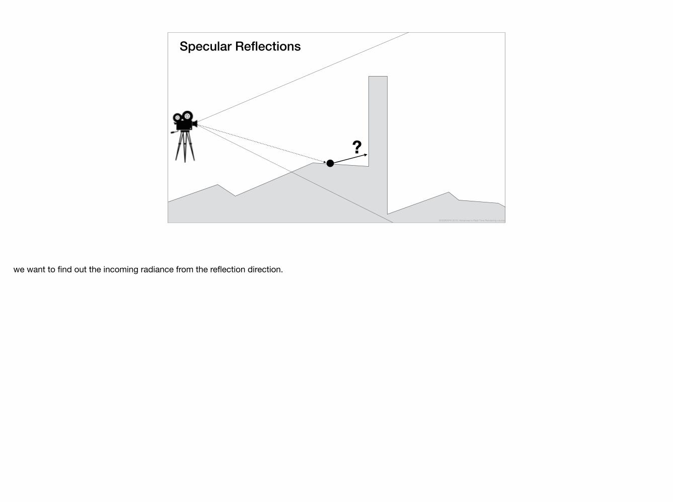
Specular Reflections
?
SIGGRAPH 2015: Advances in Real-Time Rendering course
we want to find out the incoming radiance from the reflection direction.
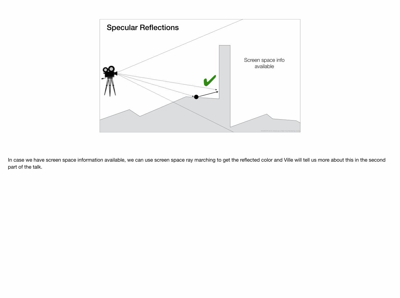
Specular Reflections
✔
Screen space info available
SIGGRAPH 2015: Advances in Real-Time Rendering course
In case we have screen space information available, we can use screen space ray marching to get the reflected color and Ville will tell us more about this in the second part of the talk.
Specular Reflections
✗
SIGGRAPH 2015: Advances in Real-Time Rendering course
However, in cases where screen space information is not available,

Specular Reflections
Fall back to local reflection probes
SIGGRAPH 2015: Advances in Real-Time Rendering course
we fall back to local reflection probes, like many other recent titles.
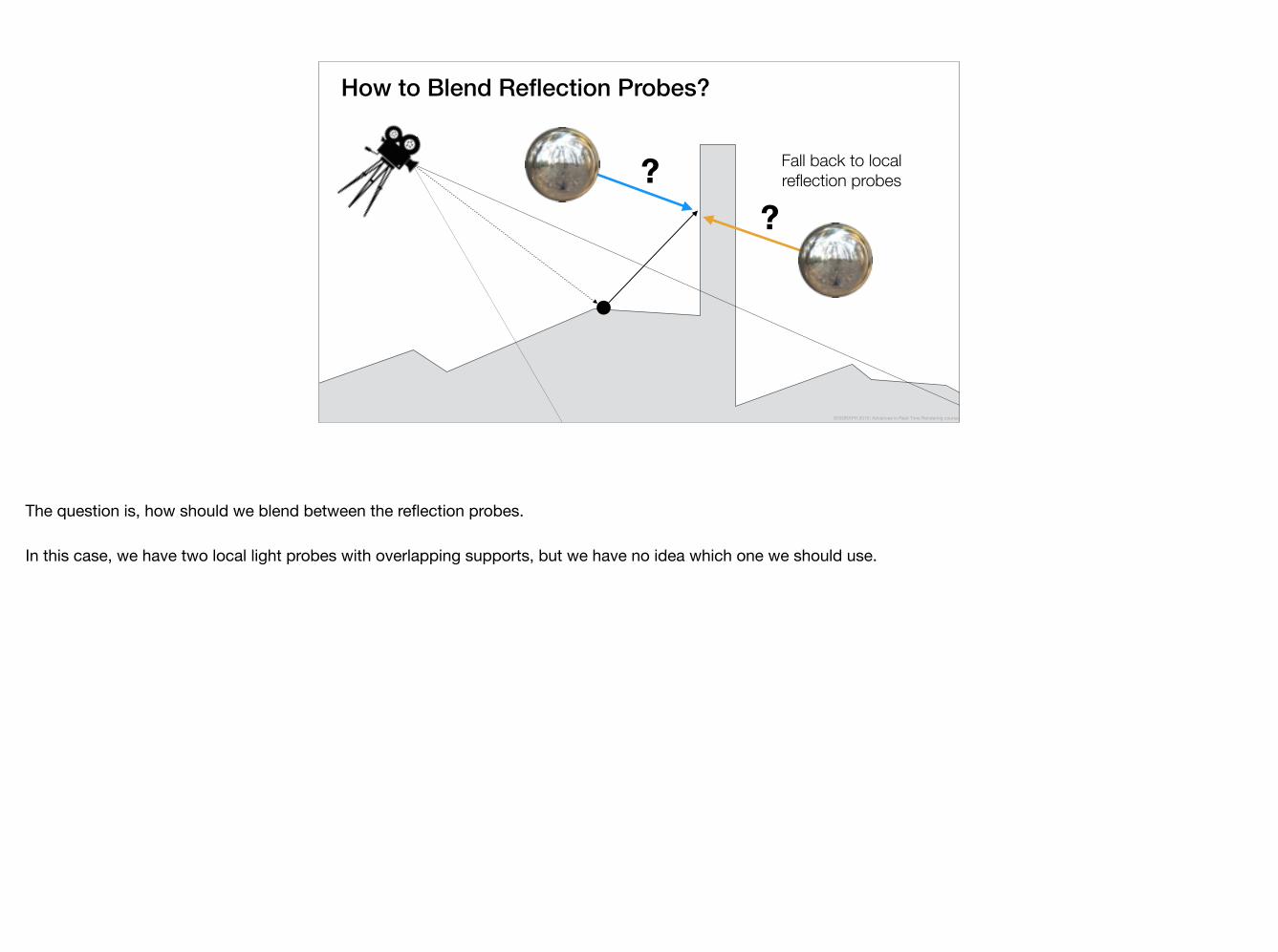
How to Blend Reflection Probes?
?? Fall back to local
reflection probes
SIGGRAPH 2015: Advances in Real-Time Rendering course
The question is, how should we blend between the reflection probes.
In this case, we have two local light probes with overlapping supports, but we have no idea which one we should use.
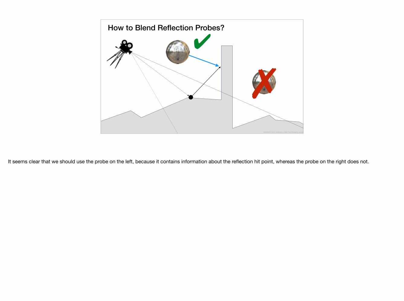
How to Blend Reflection Probes?
✔
✗SIGGRAPH 2015: Advances in Real-Time Rendering course
It seems clear that we should use the probe on the left, because it contains information about the reflection hit point, whereas the probe on the right does not.
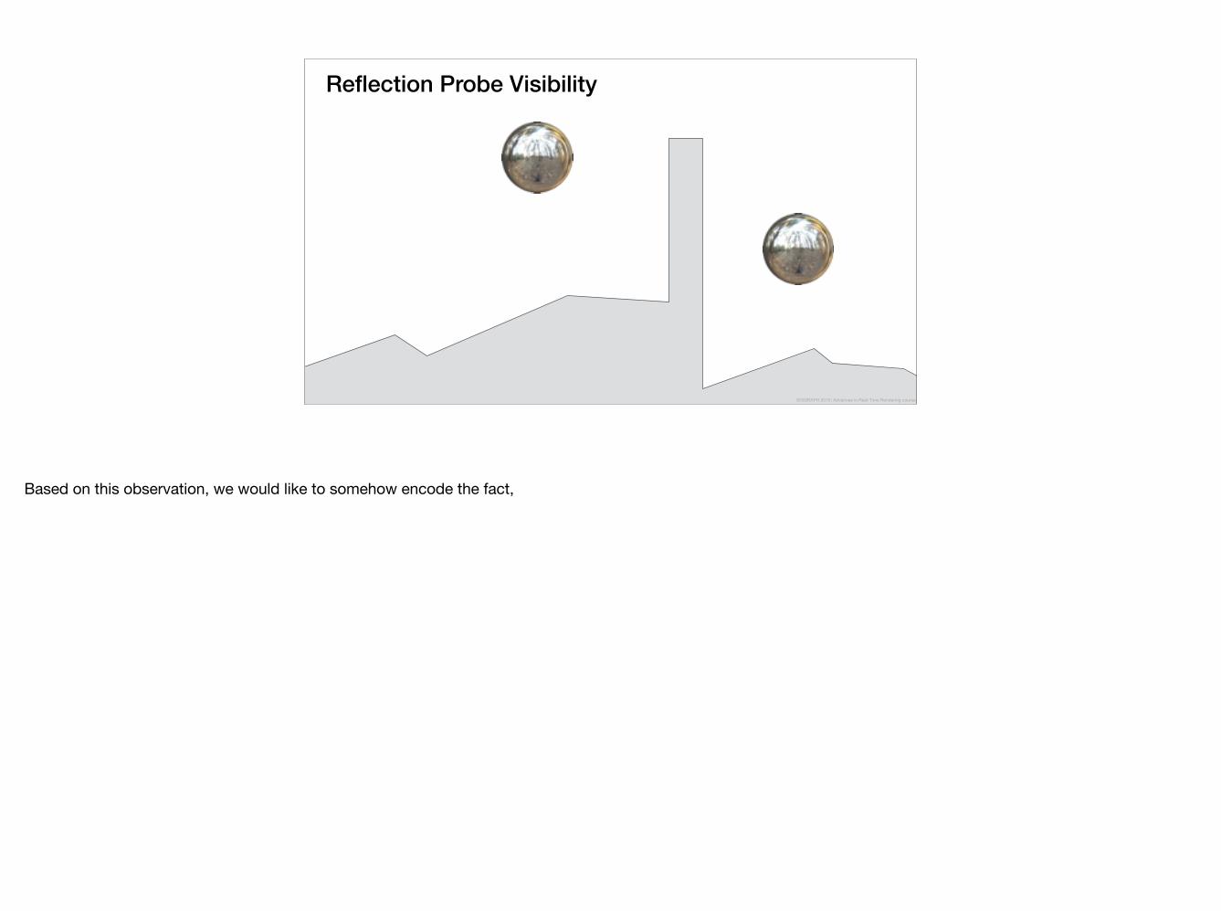
Reflection Probe Visibility
SIGGRAPH 2015: Advances in Real-Time Rendering course
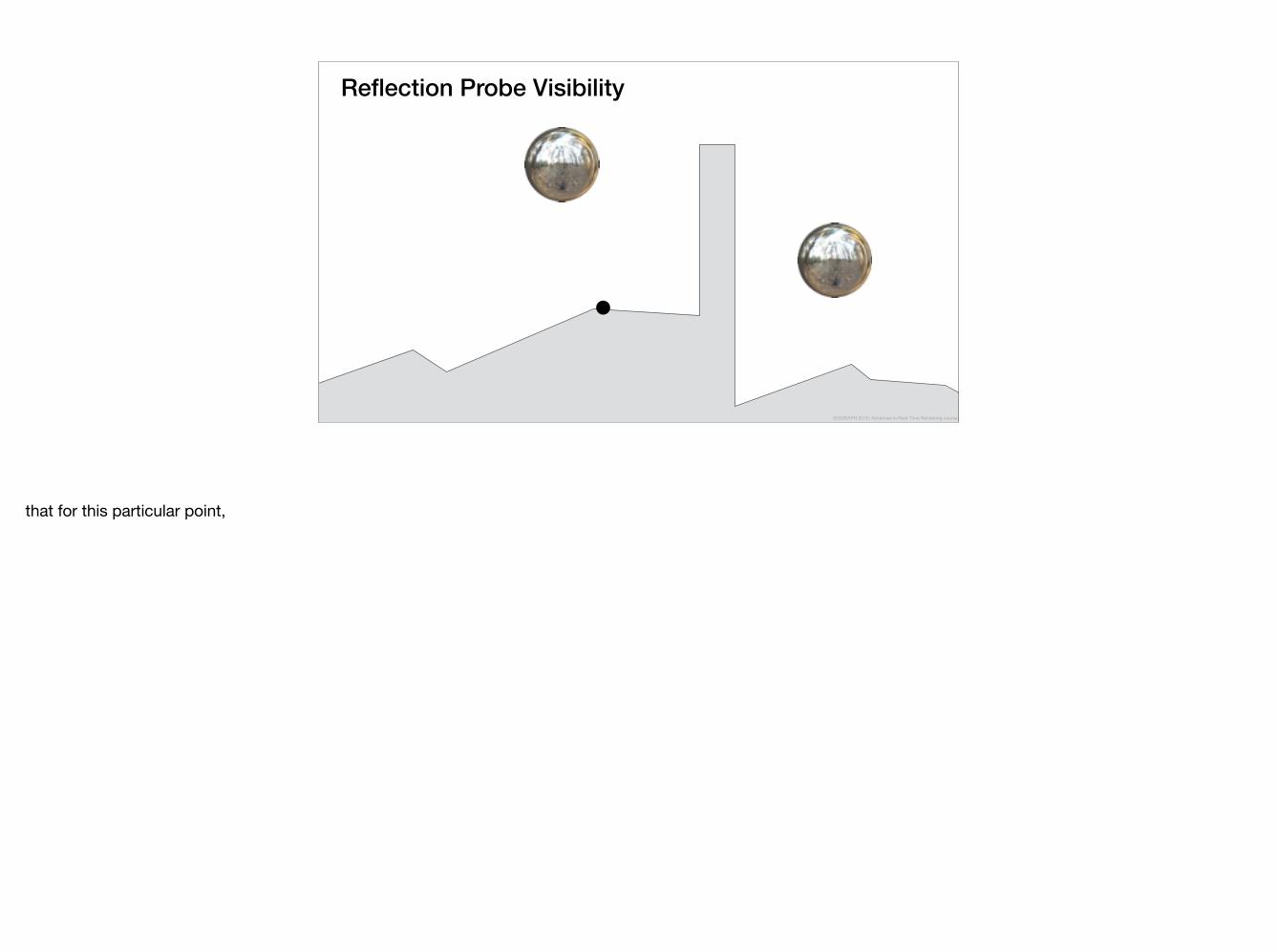
Based on this observation, we would like to somehow encode the fact,
Reflection Probe Visibility
SIGGRAPH 2015: Advances in Real-Time Rendering course
that for this particular point,
Reflection Probe Visibility
SIGGRAPH 2015: Advances in Real-Time Rendering course
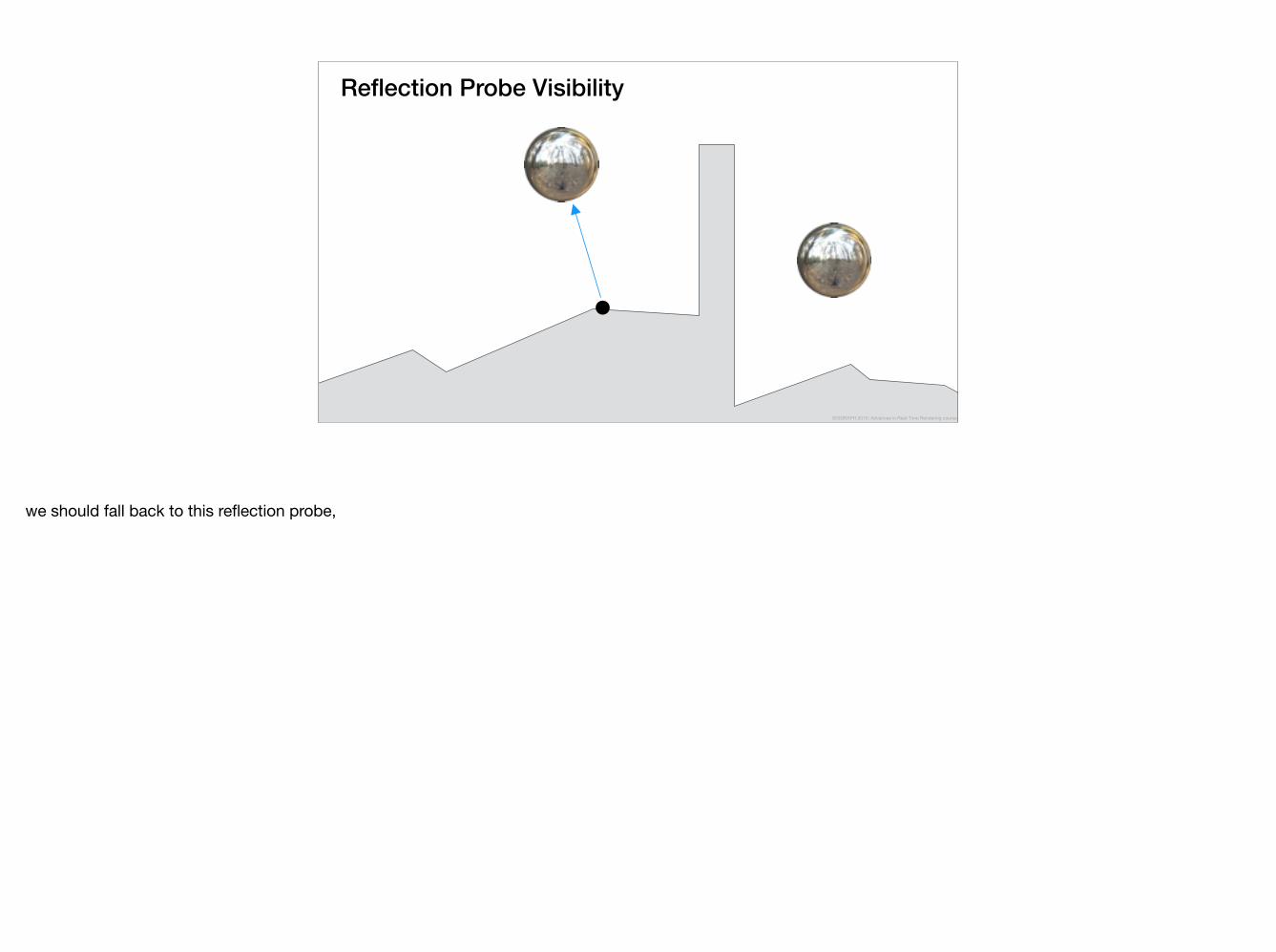
we should fall back to this reflection probe,
Reflection Probe Visibility
SIGGRAPH 2015: Advances in Real-Time Rendering course
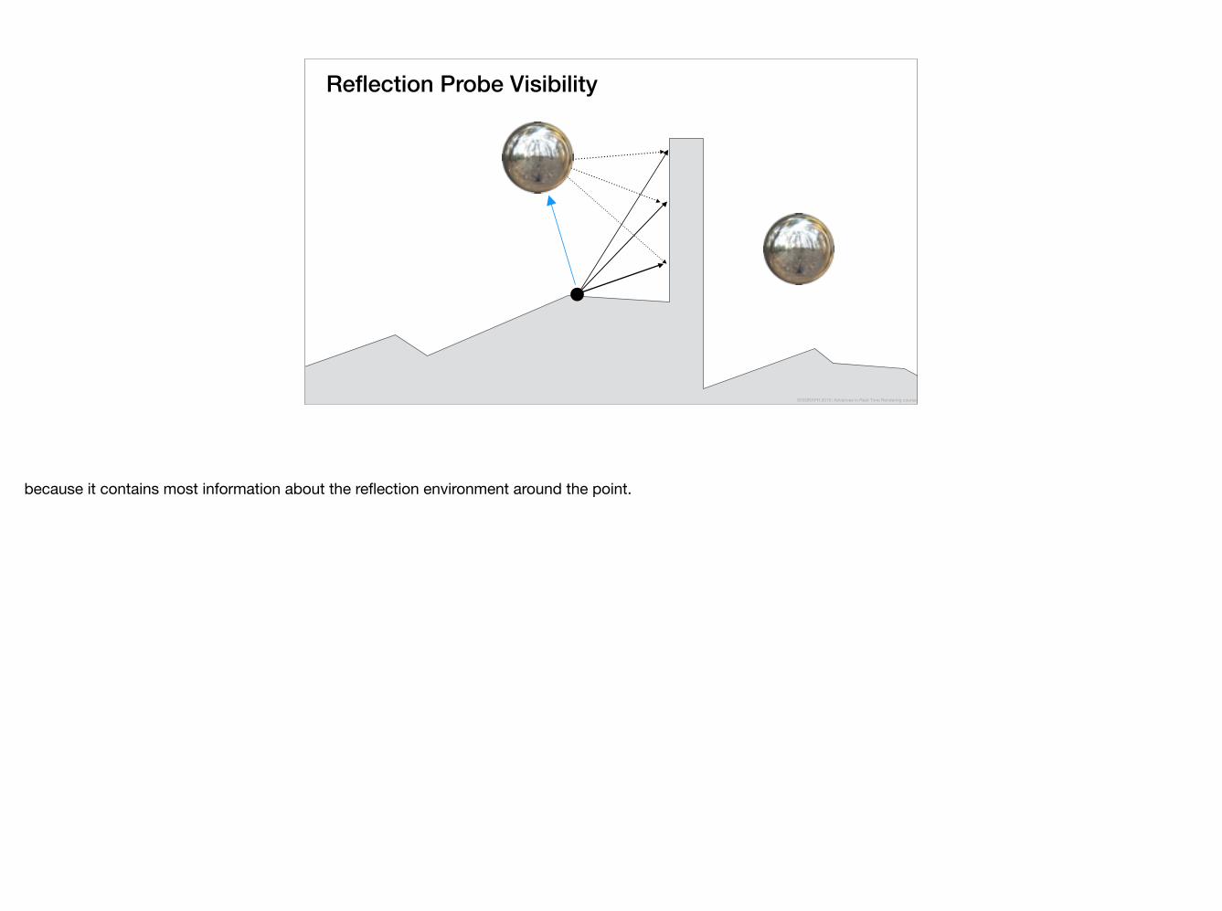
because it contains most information about the reflection environment around the point.
Reflection Probe Visibility
SIGGRAPH 2015: Advances in Real-Time Rendering course
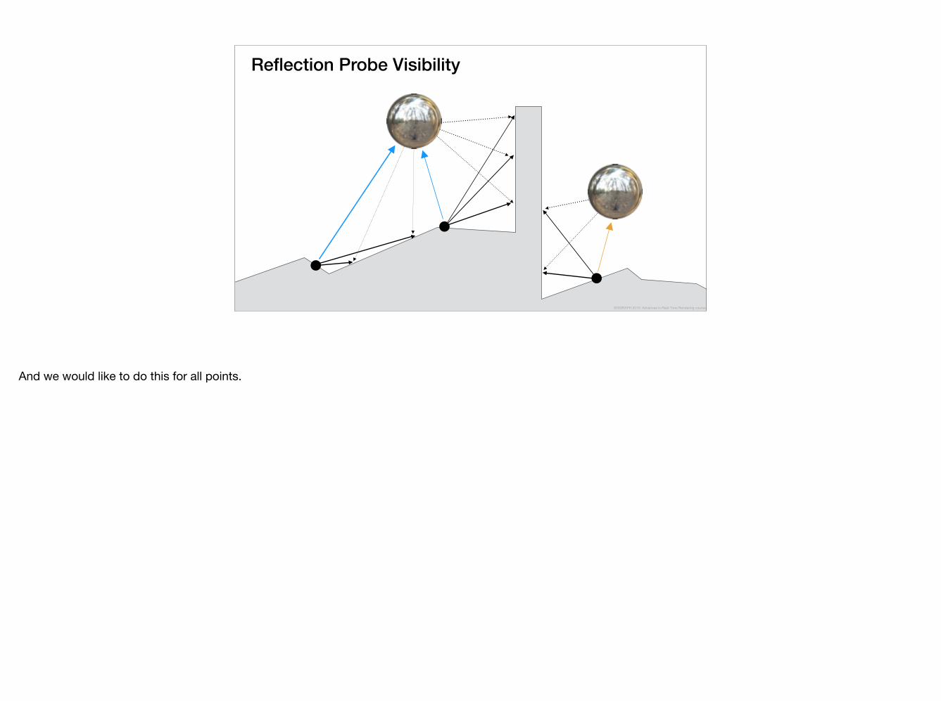
And we would like to do this for all points.

Reflection Probe Visibility
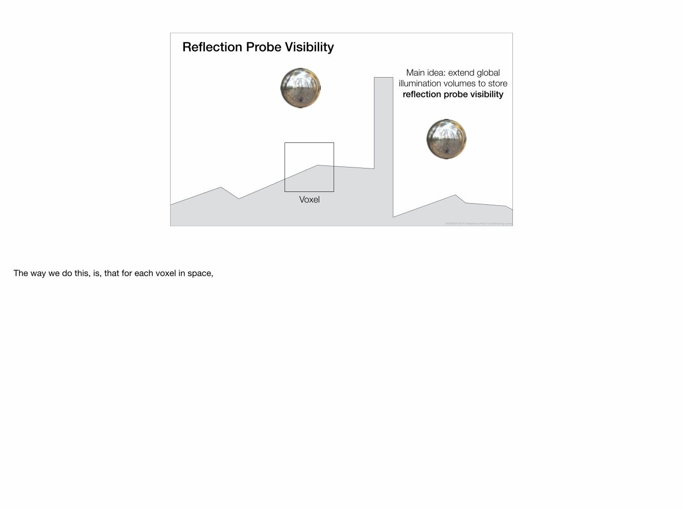
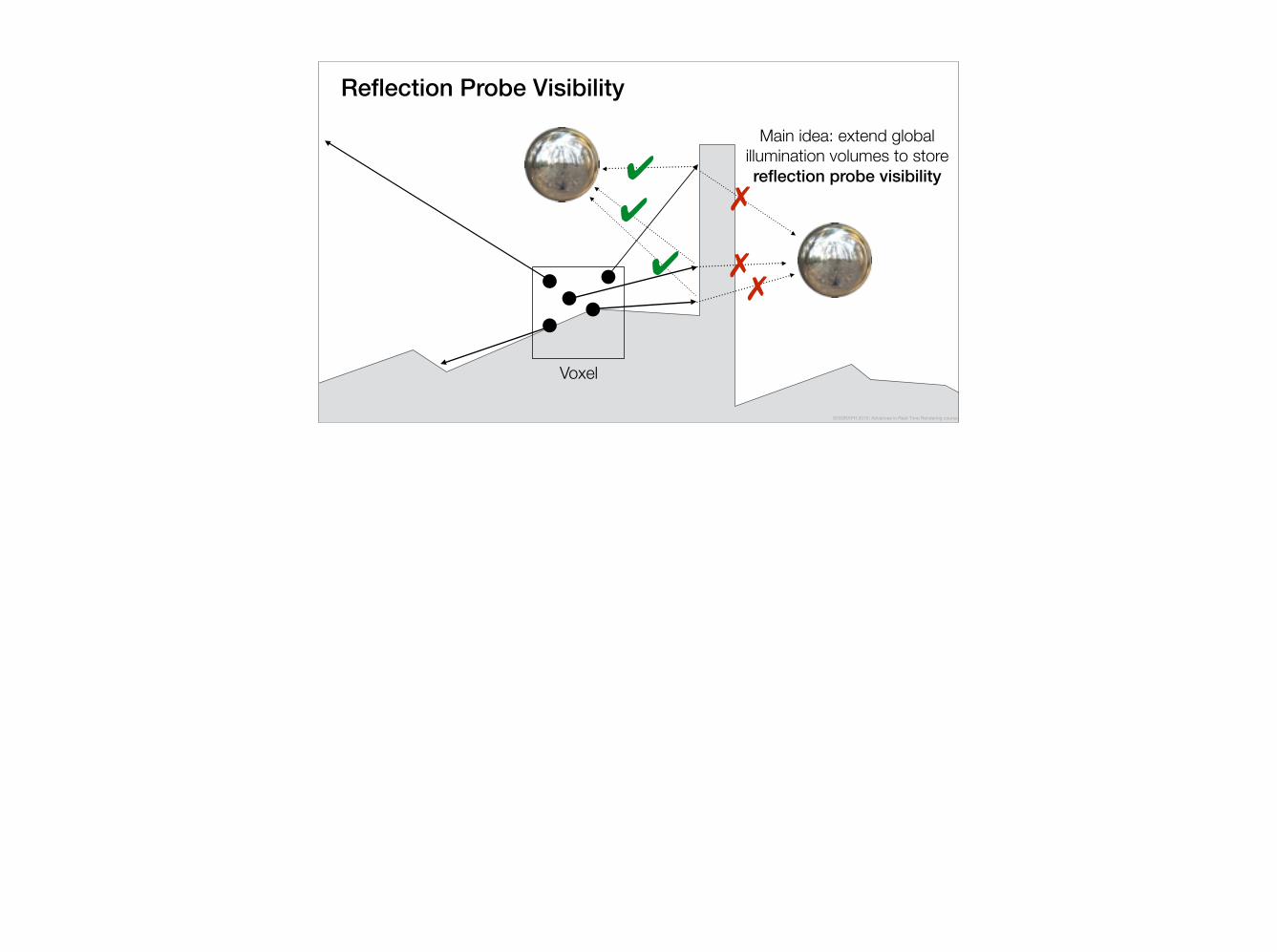
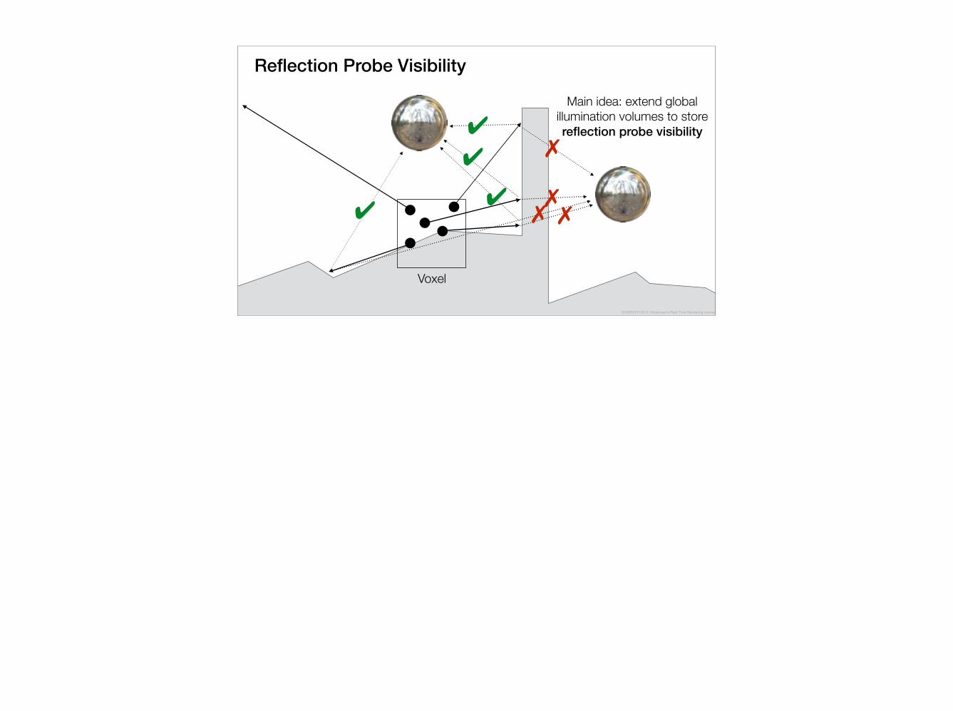
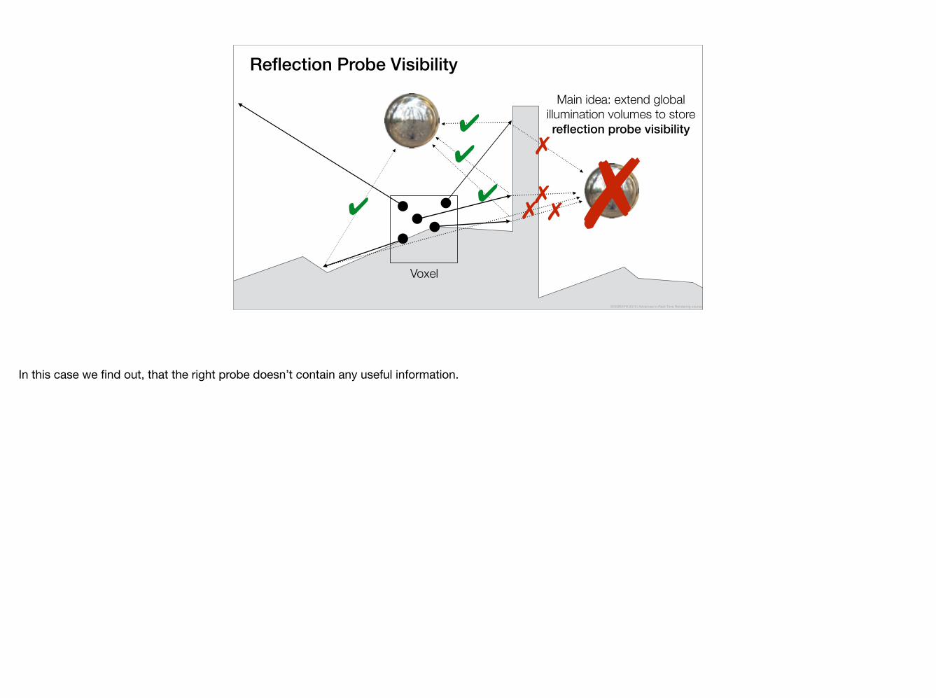
Main idea: extend global illumination volumes to store reflection probe visibility
SIGGRAPH 2015: Advances in Real-Time Rendering course
In order to do this, our main idea was to extend the global illumination volumes to store reflection probe visibility.
Reflection Probe Visibility
Voxel
Main idea: extend global illumination volumes to store reflection probe visibility
SIGGRAPH 2015: Advances in Real-Time Rendering course
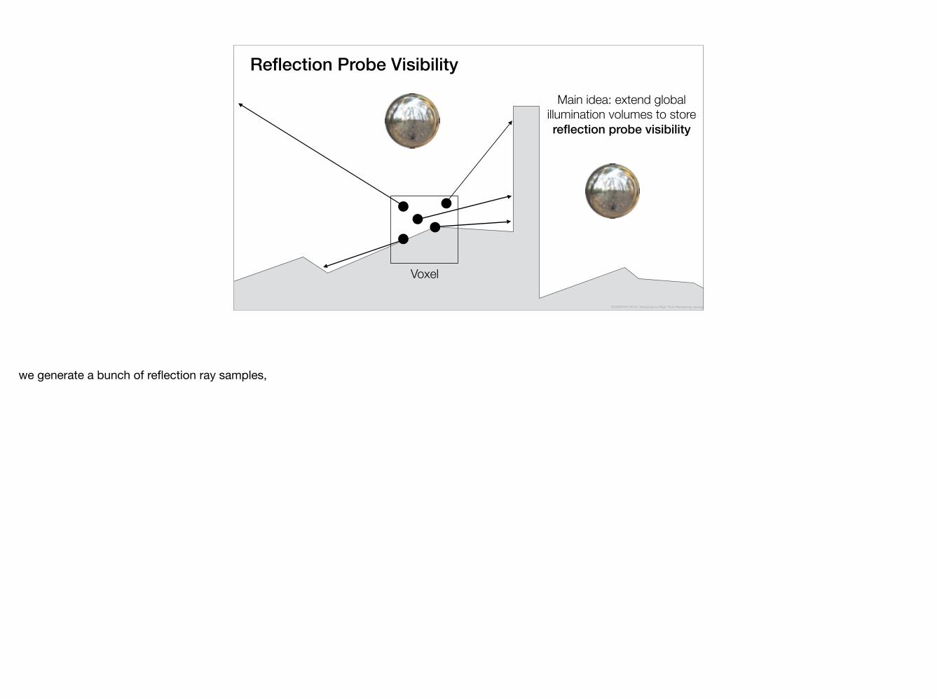
The way we do this, is, that for each voxel in space,
Reflection Probe Visibility
Voxel
Main idea: extend global illumination volumes to store reflection probe visibility
SIGGRAPH 2015: Advances in Real-Time Rendering course
we generate a bunch of reflection ray samples,
Reflection Probe Visibility
Voxel
Main idea: extend global illumination volumes to store reflection probe visibility
✗✔
SIGGRAPH 2015: Advances in Real-Time Rendering course
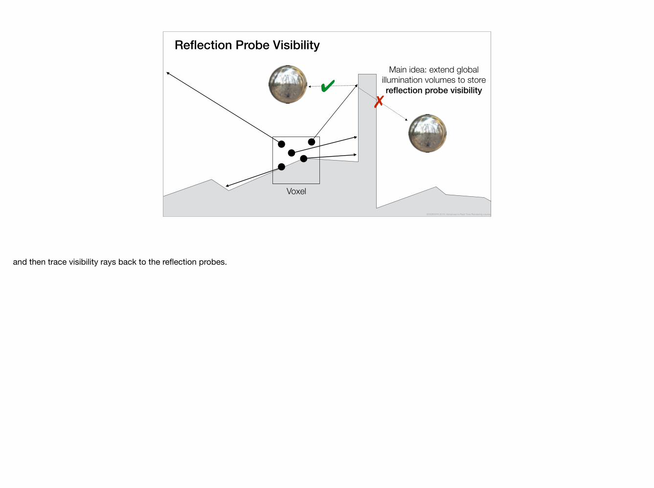
and then trace visibility rays back to the reflection probes.
Reflection Probe Visibility
Voxel
Main idea: extend global illumination volumes to store reflection probe visibility
✗
✗
✔
✔
SIGGRAPH 2015: Advances in Real-Time Rendering course
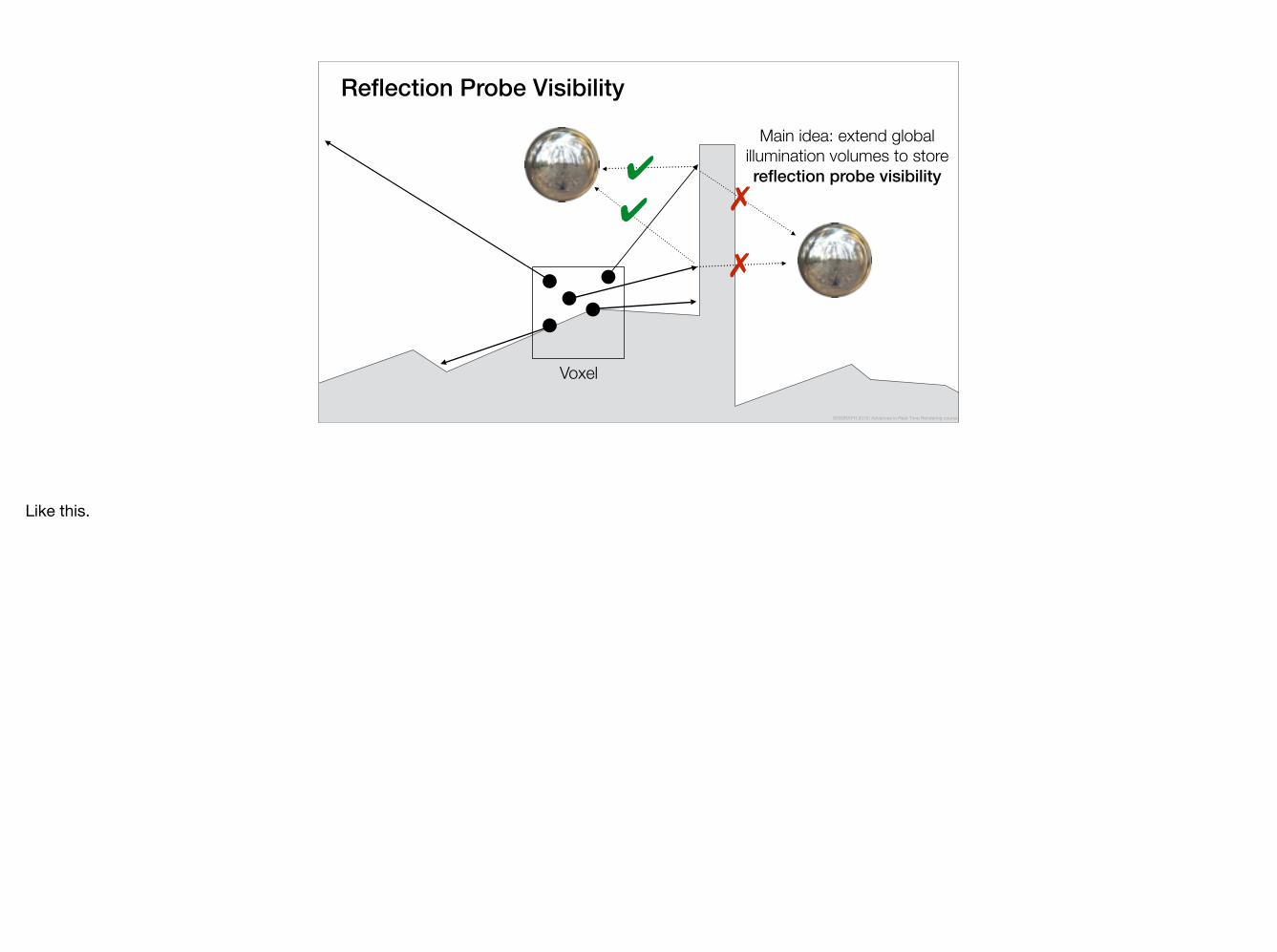
Like this.
Reflection Probe Visibility
Voxel
Main idea: extend global illumination volumes to store reflection probe visibility
✗
✗✗
✔
✔
✔
SIGGRAPH 2015: Advances in Real-Time Rendering course
Reflection Probe Visibility
Voxel
Main idea: extend global illumination volumes to store reflection probe visibility
✗
✗✗ ✗✔
✔
✔
✔
SIGGRAPH 2015: Advances in Real-Time Rendering course
Reflection Probe Visibility
Voxel
Main idea: extend global illumination volumes to store reflection probe visibility
✗
✗✗ ✗✔
✔
✔
✔ ✗SIGGRAPH 2015: Advances in Real-Time Rendering course
In this case we find out, that the right probe doesn’t contain any useful information.
Reflection Probe Visibility
Voxel
Main idea: extend global illumination volumes to store reflection probe visibility
✔
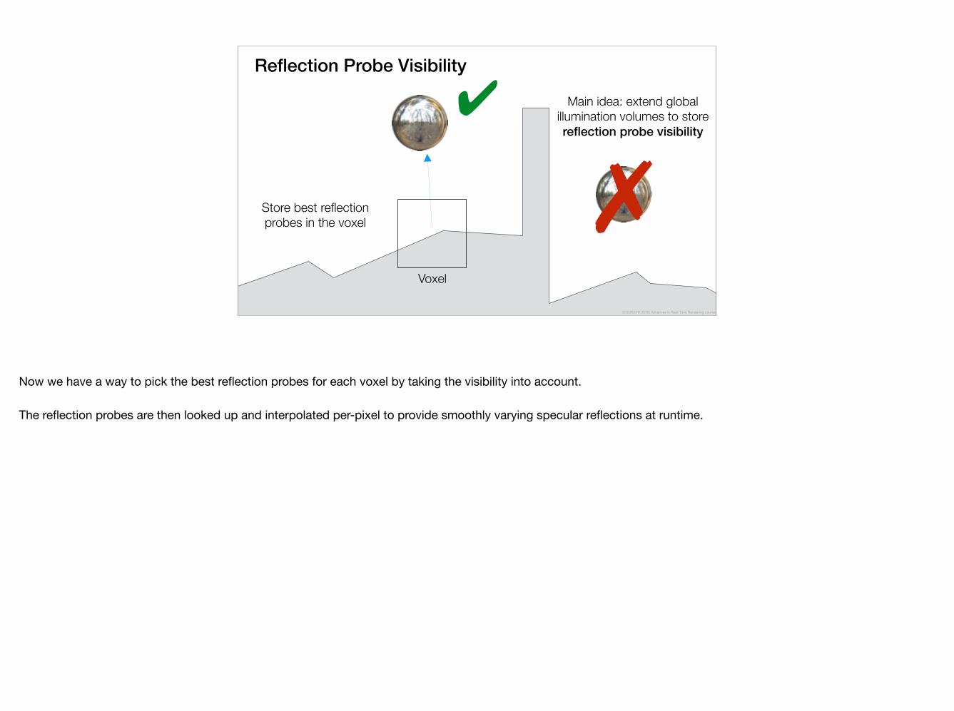
✗Store best reflection probes in the voxel
SIGGRAPH 2015: Advances in Real-Time Rendering course
Now we have a way to pick the best reflection probes for each voxel by taking the visibility into account.
The reflection probes are then looked up and interpolated per-pixel to provide smoothly varying specular reflections at runtime.
Specular Probes ON Reflection Probes
SIGGRAPH 2015: Advances in Real-Time Rendering course
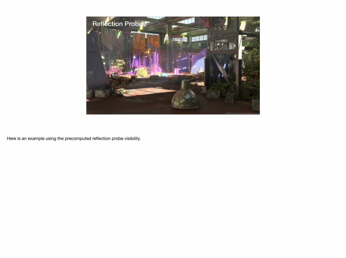
Here is an example using the precomputed reflection probe visibility.
Specular Probes OFF Reflection Probes
SIGGRAPH 2015: Advances in Real-Time Rendering course
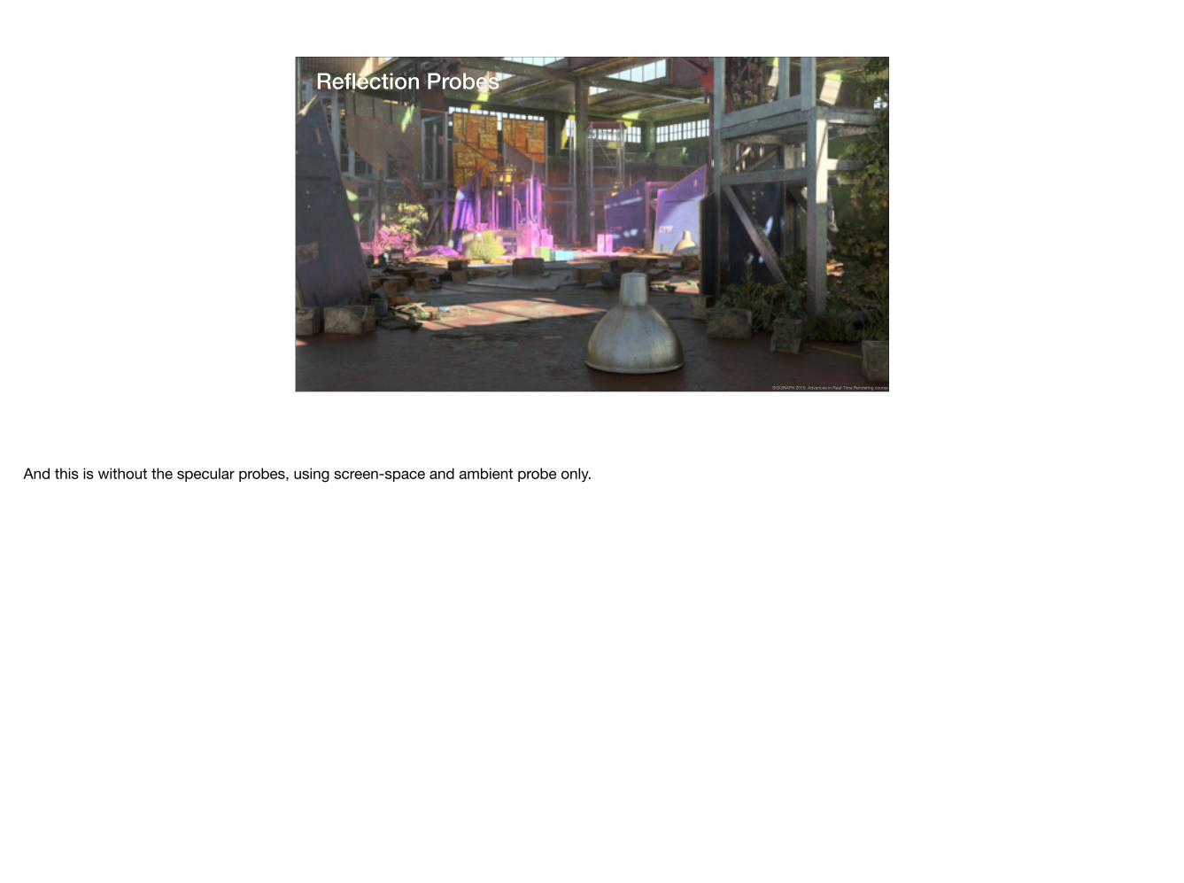
And this is without the specular probes, using screen-space and ambient probe only.
ON OffOn
SIGGRAPH 2015: Advances in Real-Time Rendering course
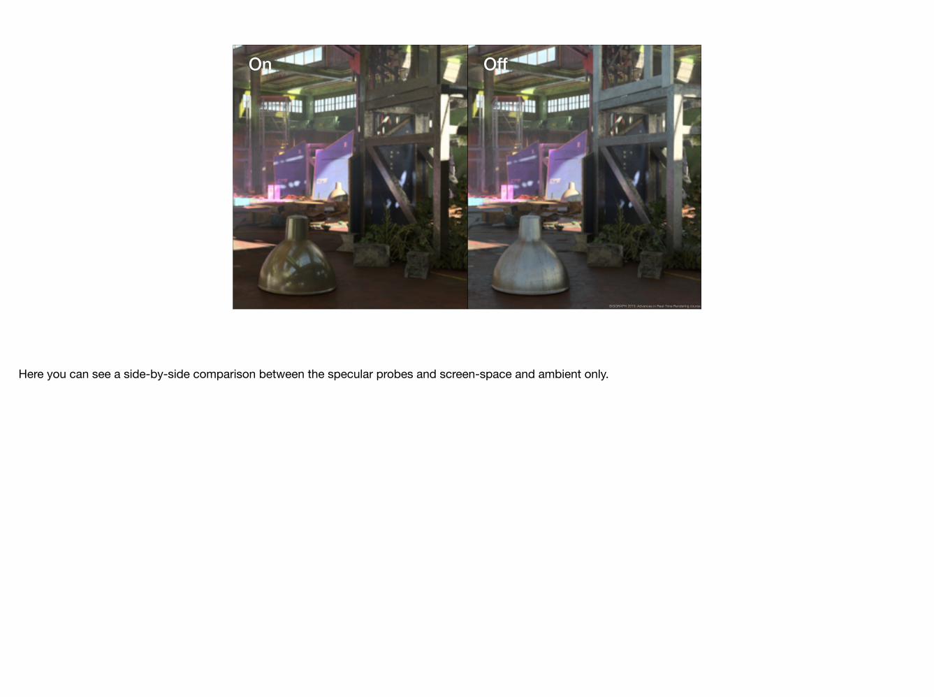
Here you can see a side-by-side comparison between the specular probes and screen-space and ambient only.
ON OffOn
SIGGRAPH 2015: Advances in Real-Time Rendering course
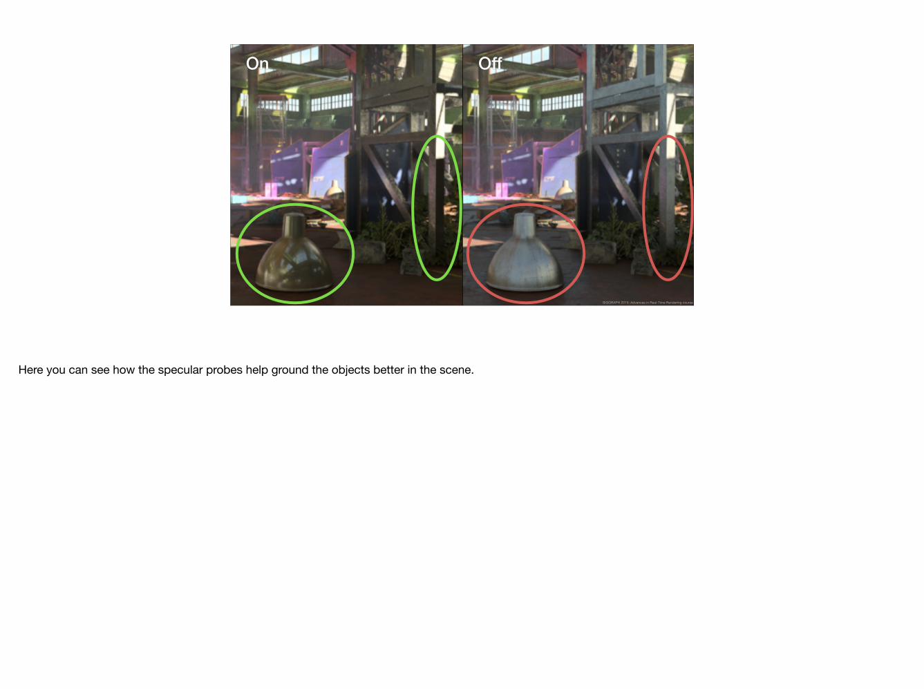
Here you can see how the specular probes help ground the objects better in the scene.
Where to Place Reflection Probes?
??
?
?
SIGGRAPH 2015: Advances in Real-Time Rendering course
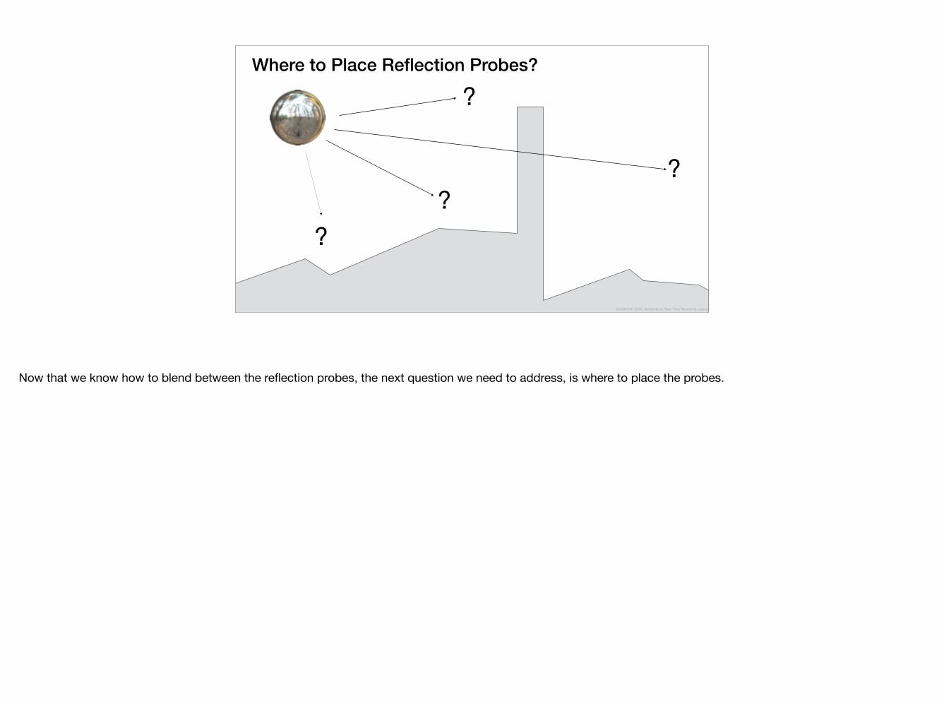
Now that we know how to blend between the reflection probes, the next question we need to address, is where to place the probes.
Where to Place Reflection Probes?
Not too close to geometry
✗ ✗ SIGGRAPH 2015: Advances in Real-Time Rendering course
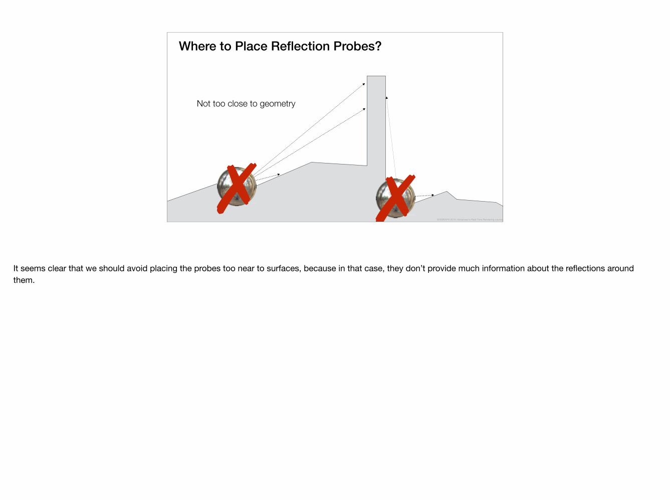
It seems clear that we should avoid placing the probes too near to surfaces, because in that case, they don’t provide much information about the reflections around them.
Where to Place Reflection Probes?
Not too far from geometry
✗
SIGGRAPH 2015: Advances in Real-Time Rendering course
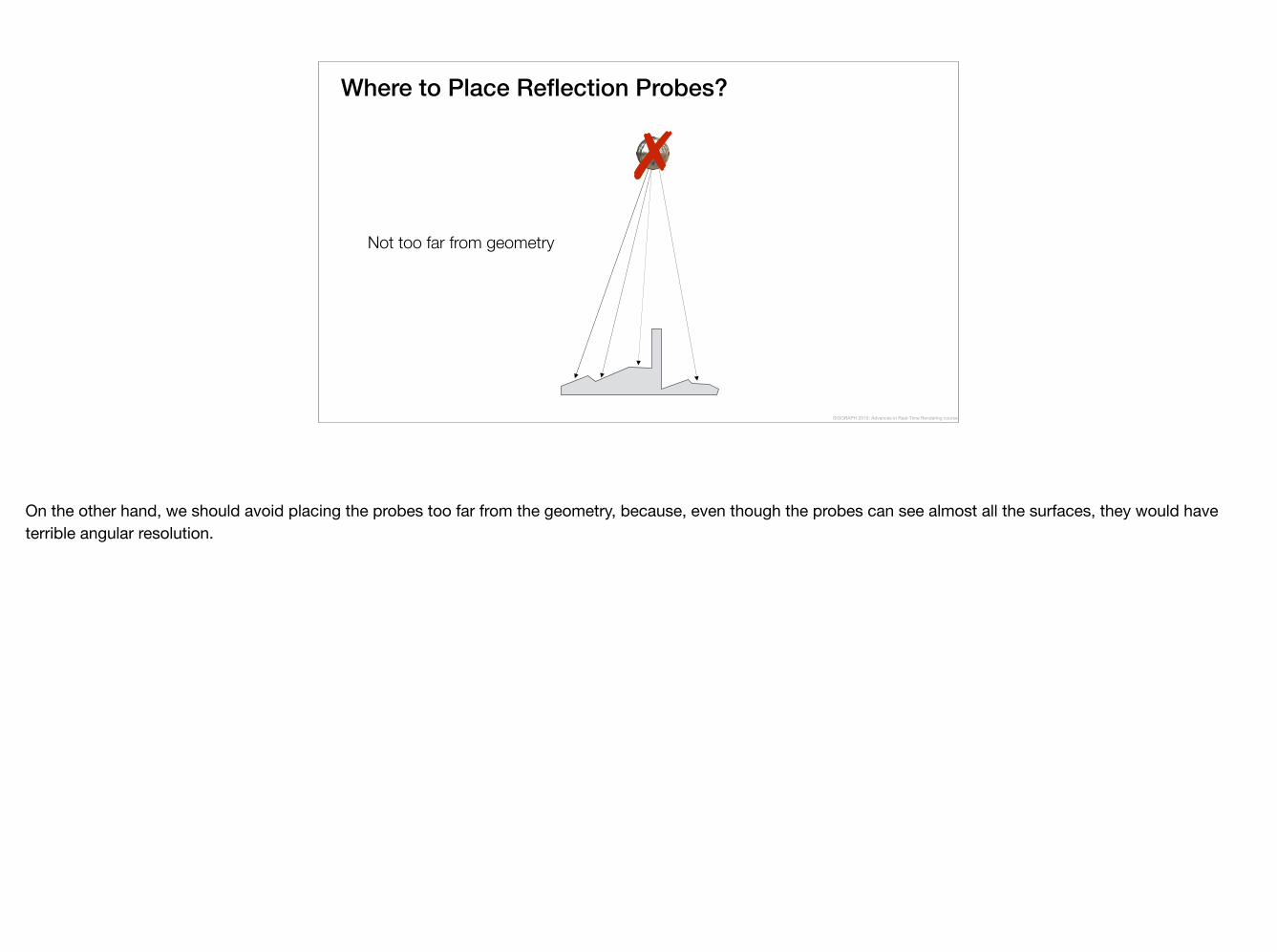
On the other hand, we should avoid placing the probes too far from the geometry, because, even though the probes can see almost all the surfaces, they would have terrible angular resolution.
Observation
Maximise visible surface area Minimize distance to surface
SIGGRAPH 2015: Advances in Real-Time Rendering course
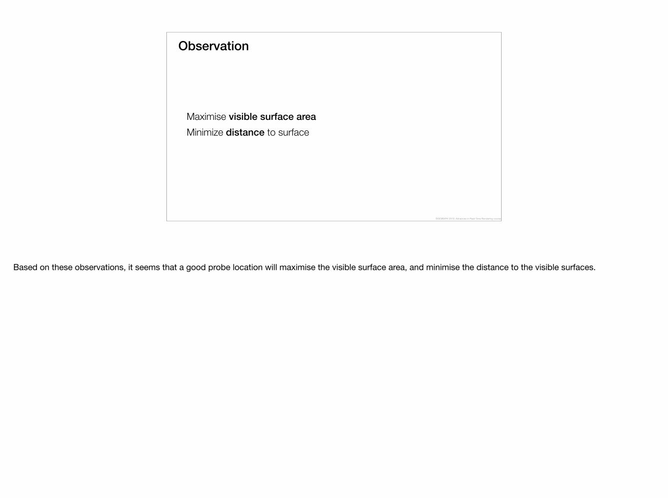
Based on these observations, it seems that a good probe location will maximise the visible surface area, and minimise the distance to the visible surfaces.
Automatic Probe Placement
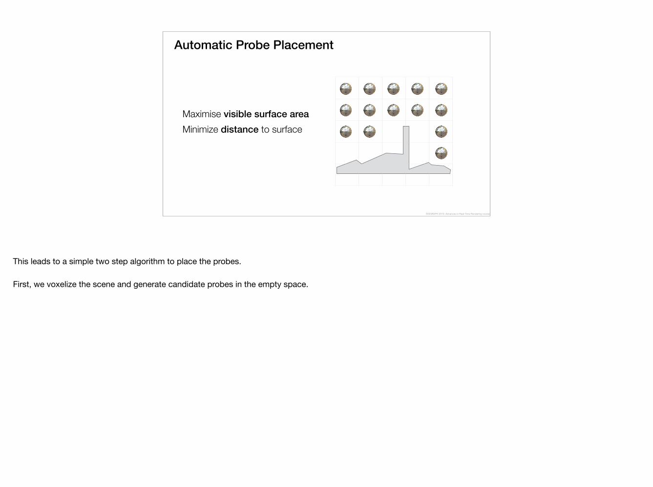
Maximise visible surface area Minimize distance to surface
SIGGRAPH 2015: Advances in Real-Time Rendering course
This leads to a simple two step algorithm to place the probes.
First, we voxelize the scene and generate candidate probes in the empty space.
Automatic Probe Placement
Maximise visible surface area Minimize distance to surface
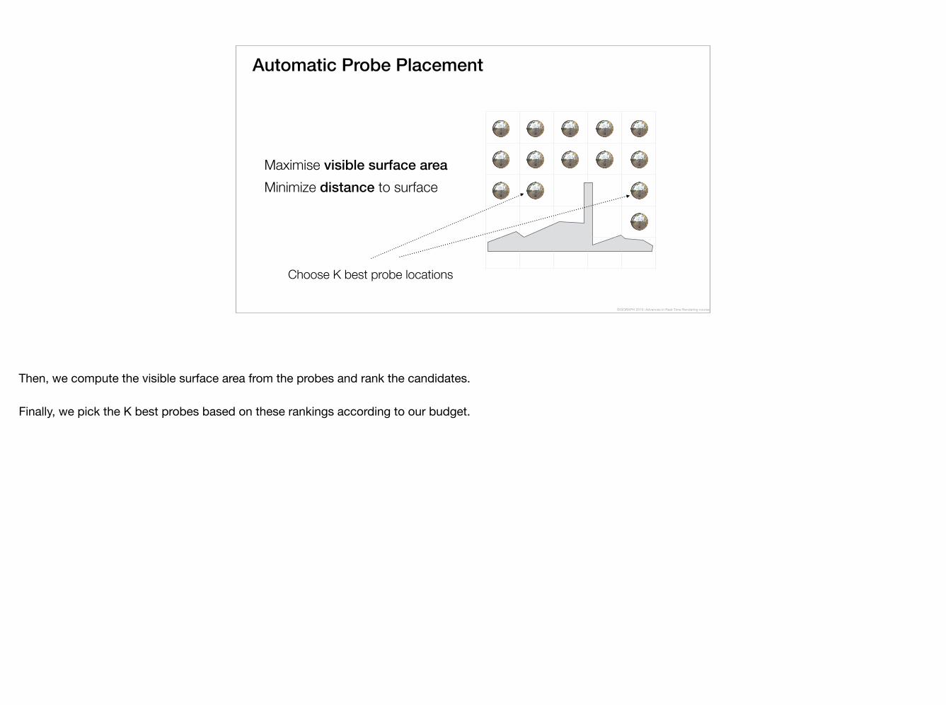
Choose K best probe locations
SIGGRAPH 2015: Advances in Real-Time Rendering course
Then, we compute the visible surface area from the probes and rank the candidates.
Finally, we pick the K best probes based on these rankings according to our budget.
Probe Placement
SIGGRAPH 2015: Advances in Real-Time Rendering course
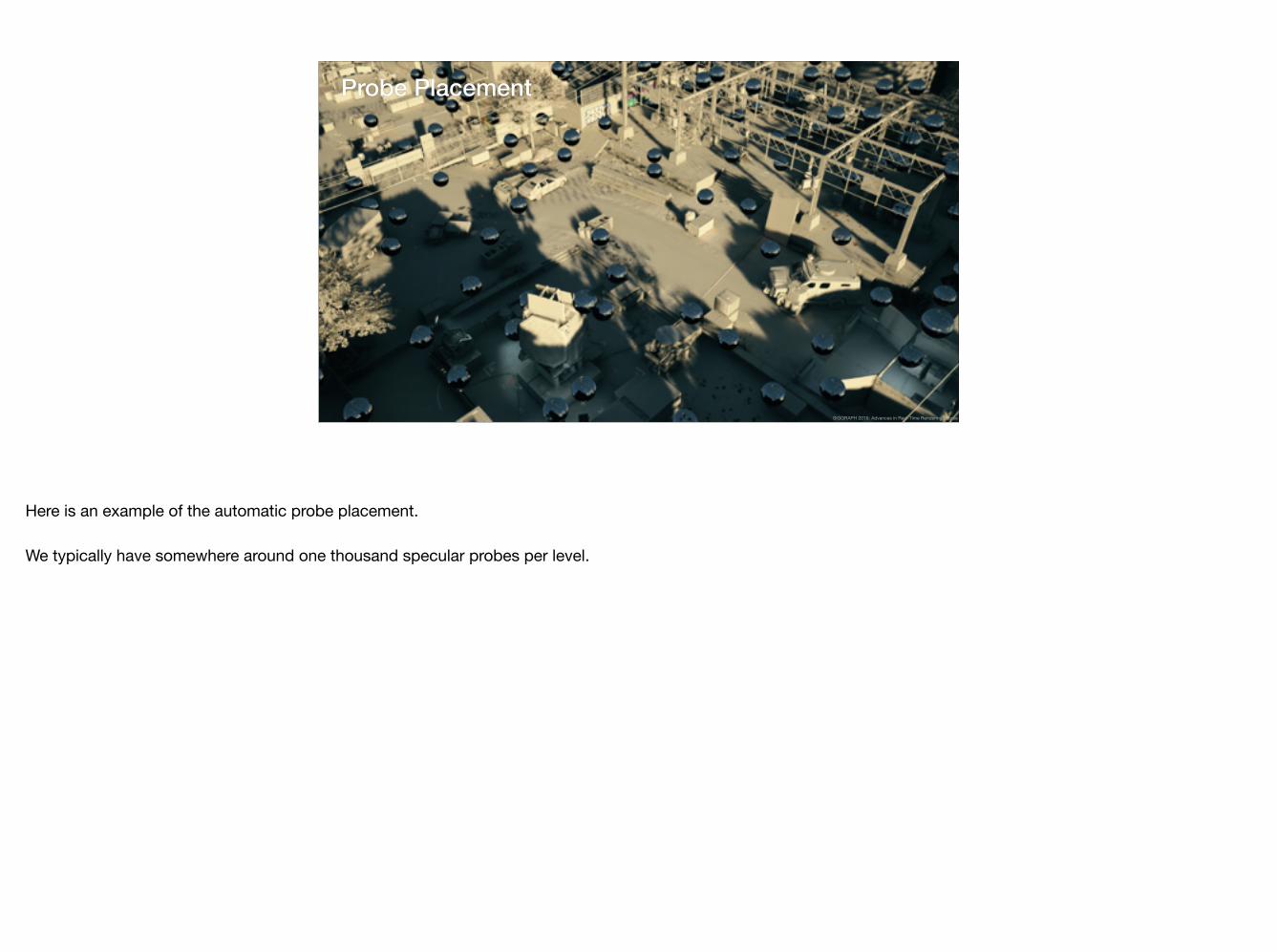
Here is an example of the automatic probe placement.
We typically have somewhere around one thousand specular probes per level.
Local Irradiance Indirect Sun Light Transport Sky Light Transport
Specular Probe Visibility Specular Probe Atlas
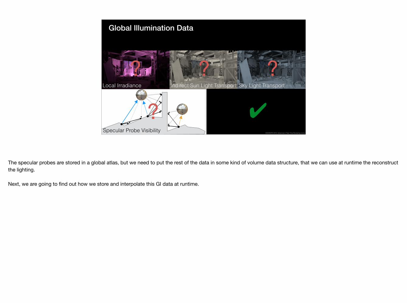
Global Illumination Data
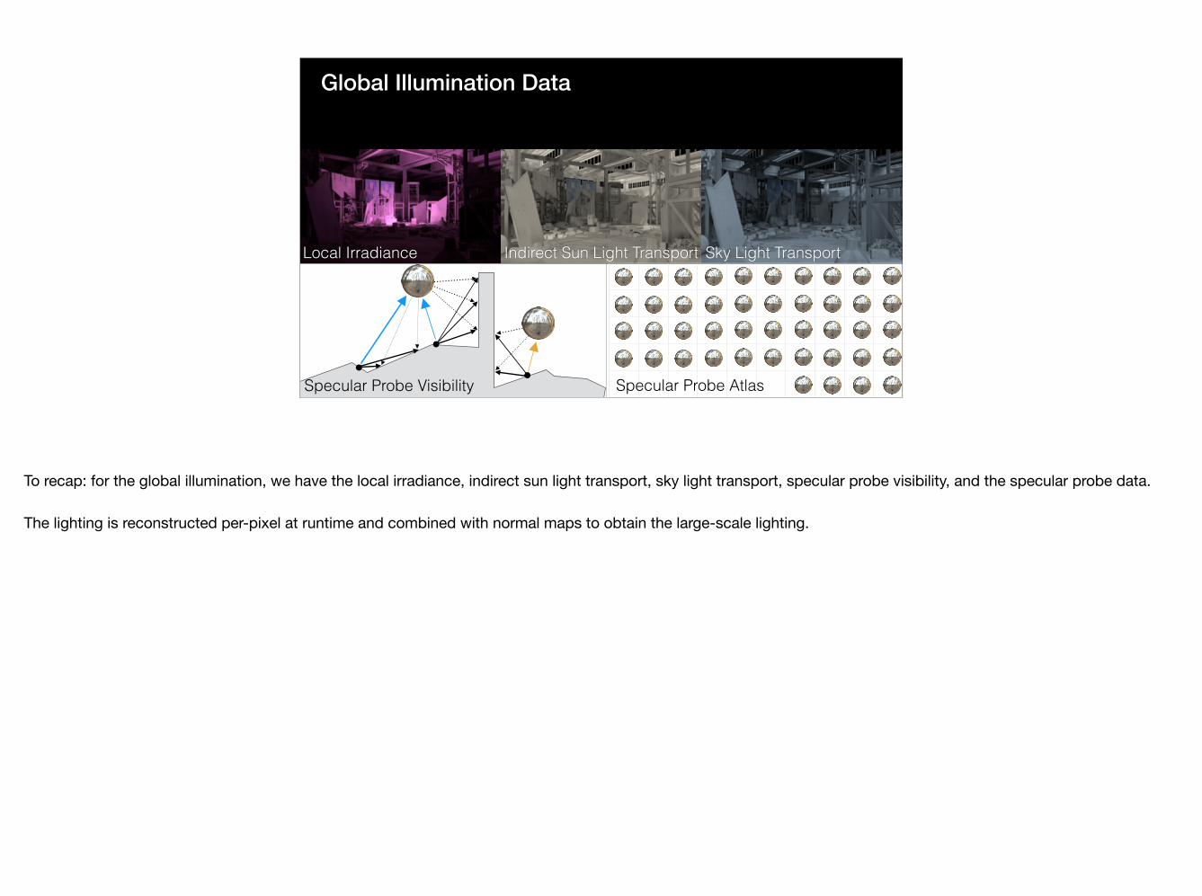
To recap: for the global illumination, we have the local irradiance, indirect sun light transport, sky light transport, specular probe visibility, and the specular probe data.
The lighting is reconstructed per-pixel at runtime and combined with normal maps to obtain the large-scale lighting.
Specular Probe Atlas
Global Illumination Data
✔
? ? ?
?Local Irradiance Indirect Sun Light Transport Sky Light Transport
Specular Probe VisibilitySIGGRAPH 2015: Advances in Real-Time Rendering course
The specular probes are stored in a global atlas, but we need to put the rest of the data in some kind of volume data structure, that we can use at runtime the reconstruct the lighting.
Next, we are going to find out how we store and interpolate this GI data at runtime.
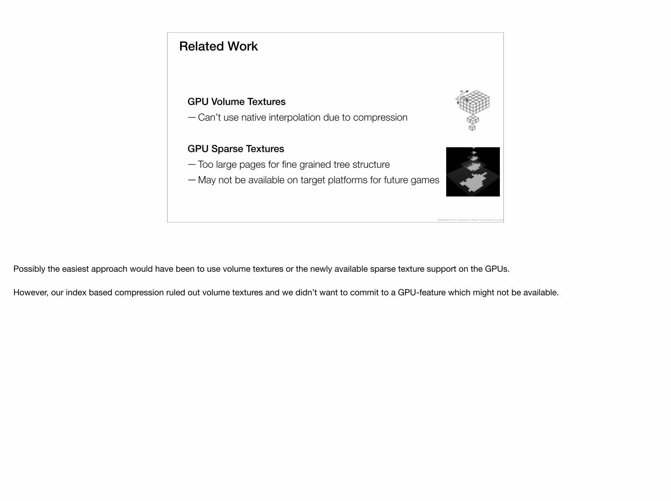
GPU Volume Textures —Can’t use native interpolation due to compression
Related Work
GPU Sparse Textures —Too large pages for fine grained tree structure —May not be available on target platforms for future games
SIGGRAPH 2015: Advances in Real-Time Rendering course
Possibly the easiest approach would have been to use volume textures or the newly available sparse texture support on the GPUs.
However, our index based compression ruled out volume textures and we didn’t want to commit to a GPU-feature which might not be available.
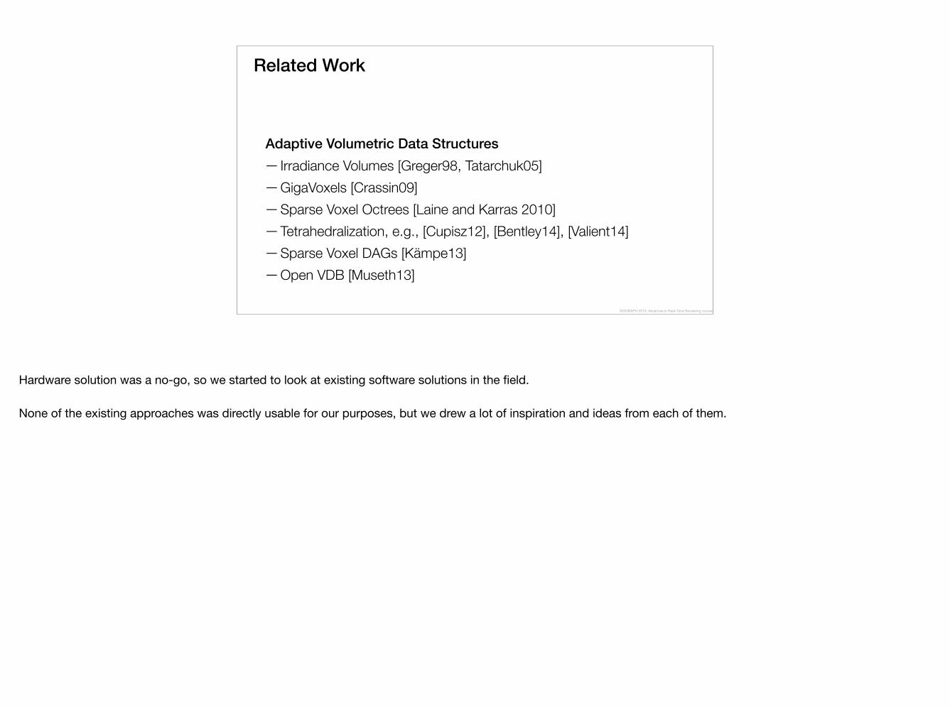
Adaptive Volumetric Data Structures —Irradiance Volumes [Greger98, Tatarchuk05] —GigaVoxels [Crassin09] —Sparse Voxel Octrees [Laine and Karras 2010] —Tetrahedralization, e.g., [Cupisz12], [Bentley14], [Valient14] —Sparse Voxel DAGs [Kämpe13] —Open VDB [Museth13]
Related Work
SIGGRAPH 2015: Advances in Real-Time Rendering course
Hardware solution was a no-go, so we started to look at existing software solutions in the field.
None of the existing approaches was directly usable for our purposes, but we drew a lot of inspiration and ideas from each of them.
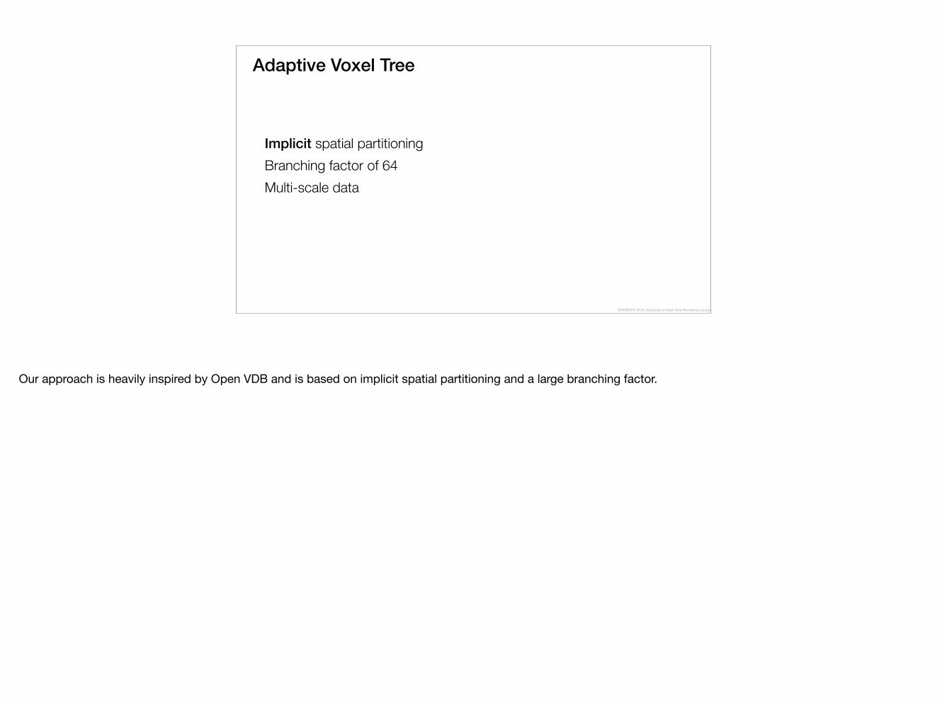
Adaptive Voxel Tree
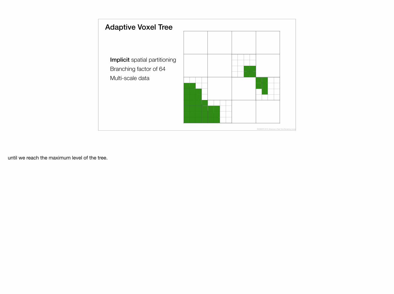
Implicit spatial partitioning Branching factor of 64 Multi-scale data
SIGGRAPH 2015: Advances in Real-Time Rendering course
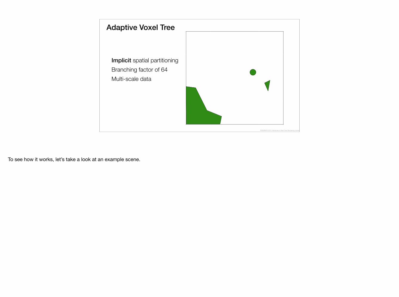
Our approach is heavily inspired by Open VDB and is based on implicit spatial partitioning and a large branching factor.
Adaptive Voxel Tree
Implicit spatial partitioning Branching factor of 64 Multi-scale data
SIGGRAPH 2015: Advances in Real-Time Rendering course
To see how it works, let’s take a look at an example scene.
Adaptive Voxel Tree
Implicit spatial partitioning Branching factor of 64 Multi-scale data
SIGGRAPH 2015: Advances in Real-Time Rendering course
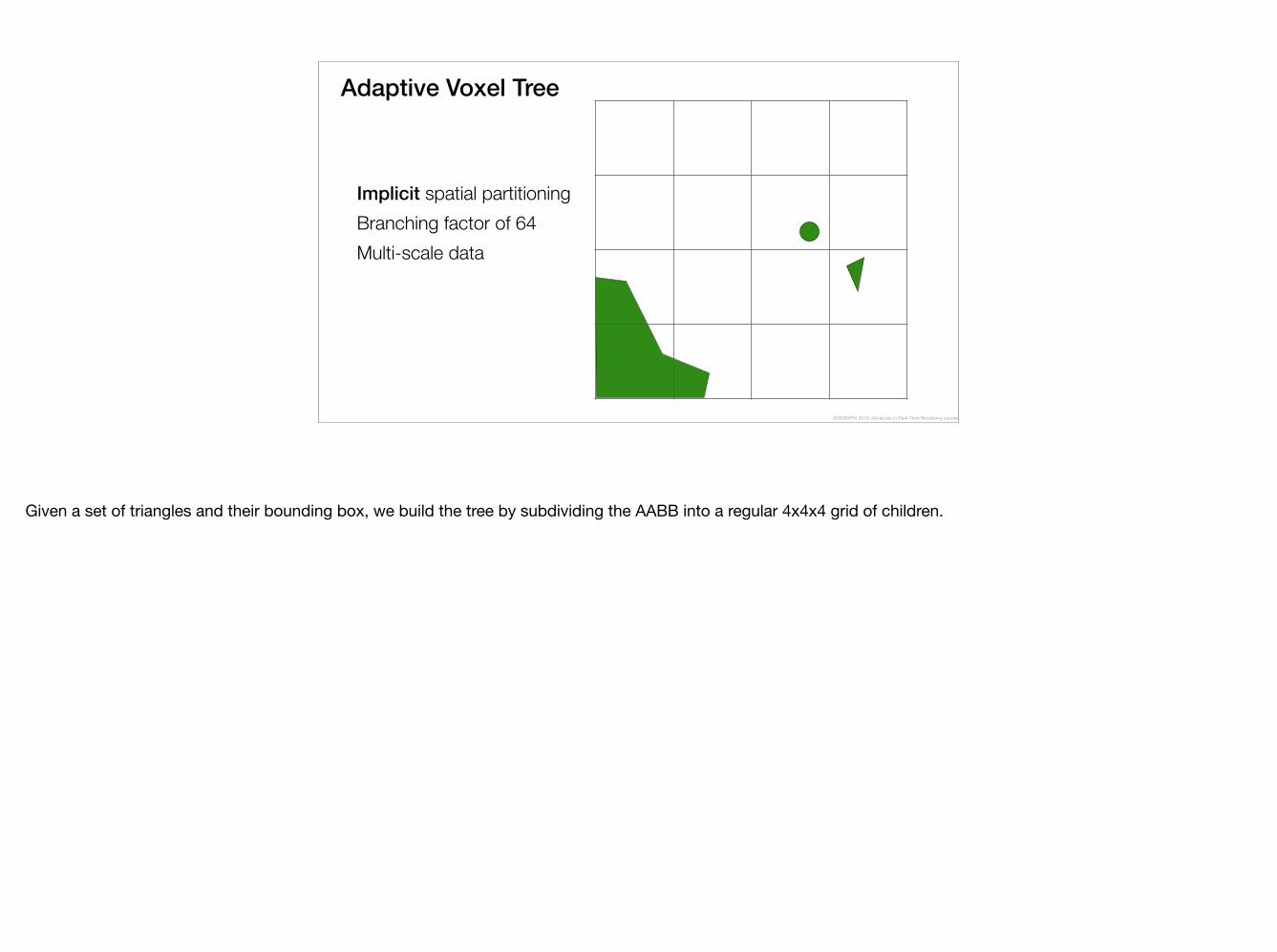
Given a set of triangles and their bounding box, we build the tree by subdividing the AABB into a regular 4x4x4 grid of children.
Adaptive Voxel Tree
Implicit spatial partitioning Branching factor of 64 Multi-scale data
SIGGRAPH 2015: Advances in Real-Time Rendering course
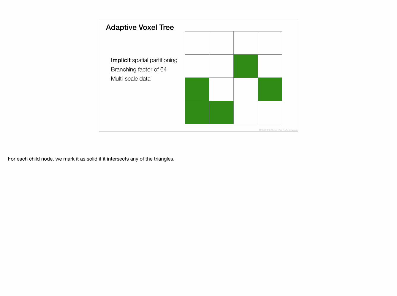
For each child node, we mark it as solid if it intersects any of the triangles.
Adaptive Voxel Tree
Implicit spatial partitioning Branching factor of 64 Multi-scale data
SIGGRAPH 2015: Advances in Real-Time Rendering course
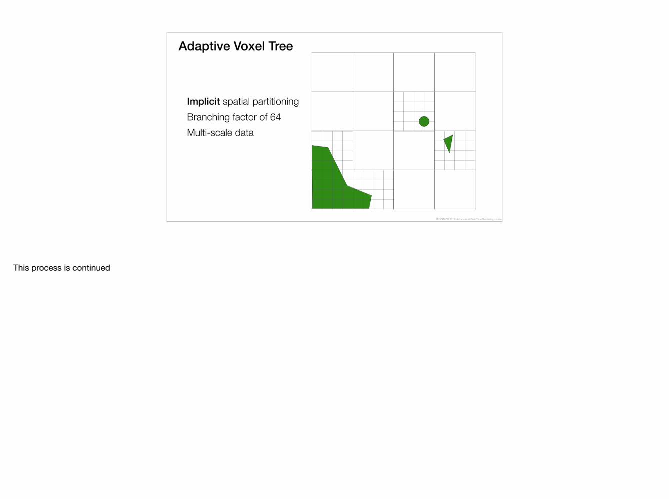
This process is continued
Adaptive Voxel Tree
Implicit spatial partitioning Branching factor of 64 Multi-scale data
SIGGRAPH 2015: Advances in Real-Time Rendering course
until we reach the maximum level of the tree.

Voxel Tree Structure
Voxel Node ArraySIGGRAPH 2015: Advances in Real-Time Rendering course
The resulting voxel tree is stored as a single linear array of voxel tree nodes in memory.
Node Structure
Child Mask
Child Block Offset
64 bits
31 bits Terminal Node Bit1 bit
Node Structure
Voxel Node ArraySIGGRAPH 2015: Advances in Real-Time Rendering course
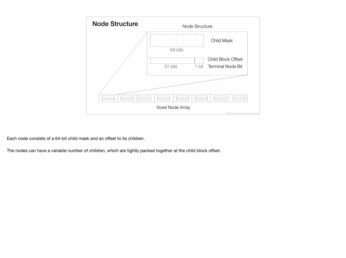
Each node consists of a 64-bit child mask and an offset to its children.
The nodes can have a variable number of children, which are tightly packed together at the child block offset.

Child Mask
12 13 14 158 9 10 114 5 6 70 1 2 3
0 1 2 3 4 5 6 78 9 10 11 12 13 14 15
Child Mask
Child Block Offset
64 bits
31 bits Terminal Node Bit1 bit
Voxel Node Array
Voxel Grid
Node Structure
SIGGRAPH 2015: Advances in Real-Time Rendering course
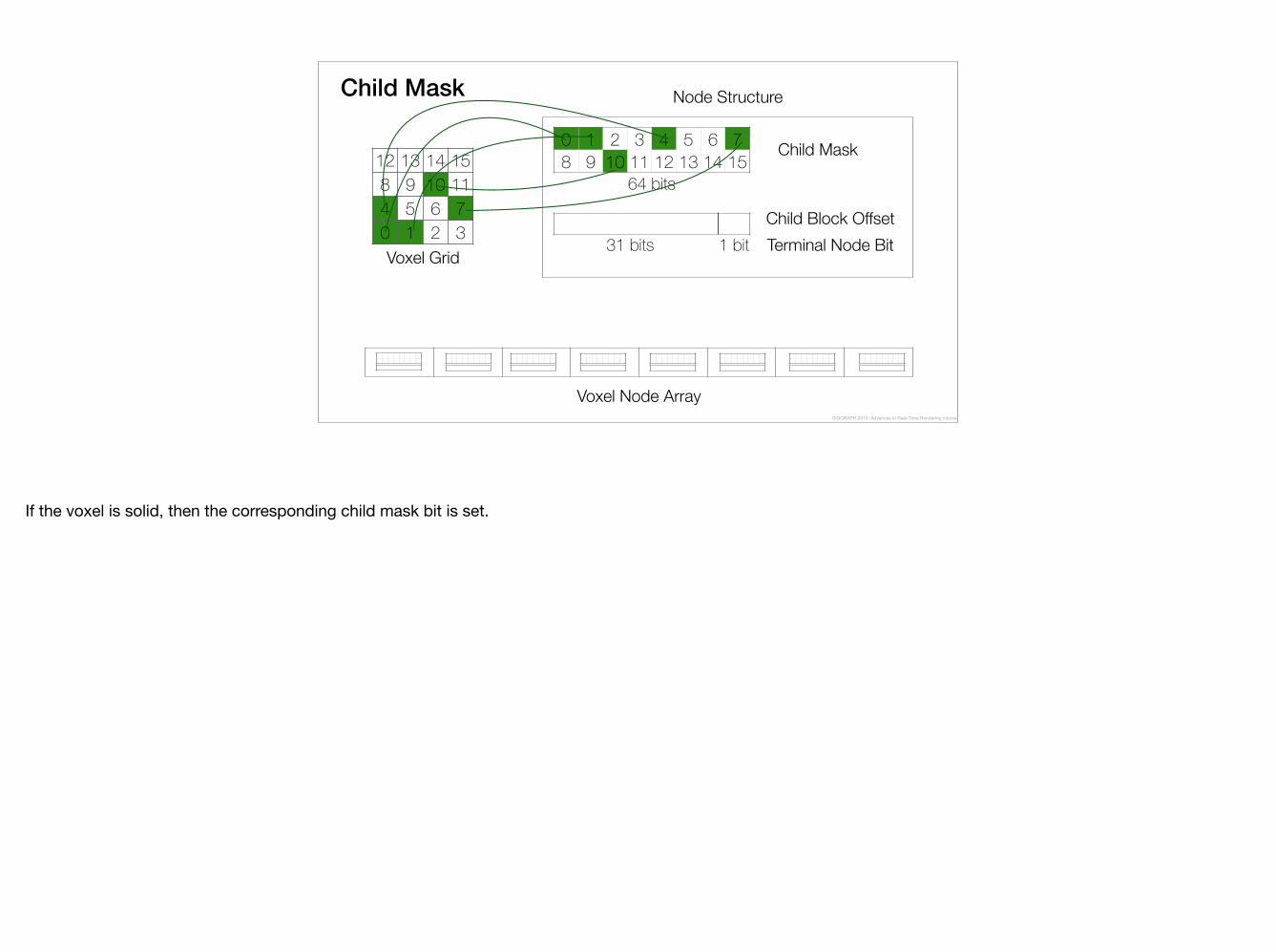
The child mask contains one bit for each voxel in the world space voxel grid of the node.
12 13 14 158 9 10 114 5 6 70 1 2 3
0 1 2 3 4 5 6 78 9 10 11 12 13 14 15
Child Mask
Child Block Offset
64 bits
31 bits Terminal Node Bit1 bit
Voxel Node Array
Voxel Grid
Node StructureChild Mask
SIGGRAPH 2015: Advances in Real-Time Rendering course
If the voxel is solid, then the corresponding child mask bit is set.
Voxel Node Array
7 Child Mask
Child Block Offset
64 bits
31 bits Terminal Node Bit1 bit
7
Voxel Grid
Node StructureTree Traversal
Child Index = ?
SIGGRAPH 2015: Advances in Real-Time Rendering course
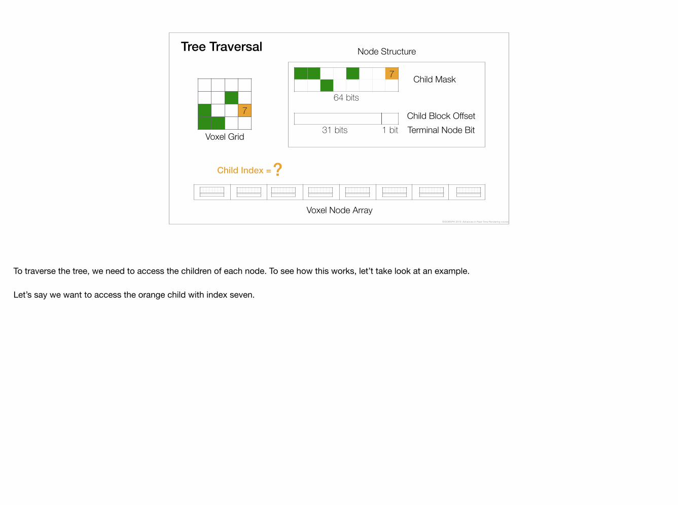
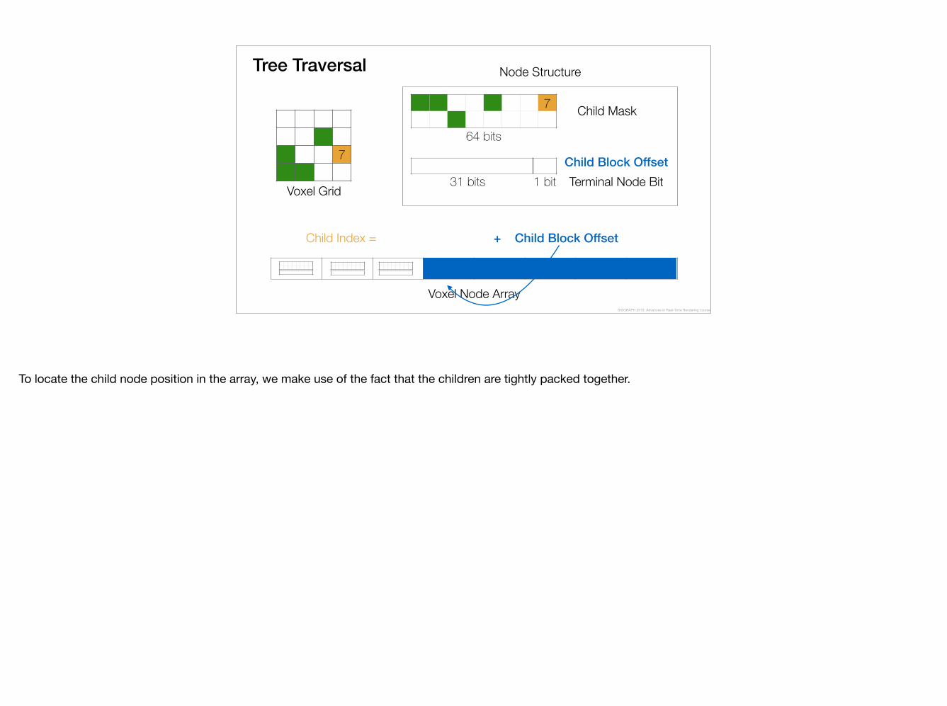
To traverse the tree, we need to access the children of each node. To see how this works, let’t take look at an example.
Let’s say we want to access the orange child with index seven.
Voxel Node Array
7 Child Mask
Child Block Offset
64 bits
31 bits Terminal Node Bit1 bit
7
Voxel Grid
Node StructureTree Traversal
+ Child Block OffsetChild Index =
SIGGRAPH 2015: Advances in Real-Time Rendering course
To locate the child node position in the array, we make use of the fact that the children are tightly packed together.
Voxel Node Array
7 Child Mask
Child Block Offset
64 bits
31 bits Terminal Node Bit1 bit
7
Voxel Grid
Node StructureTree Traversal
+ Child Block Offset3 set bitsChild Index =
SIGGRAPH 2015: Advances in Real-Time Rendering course
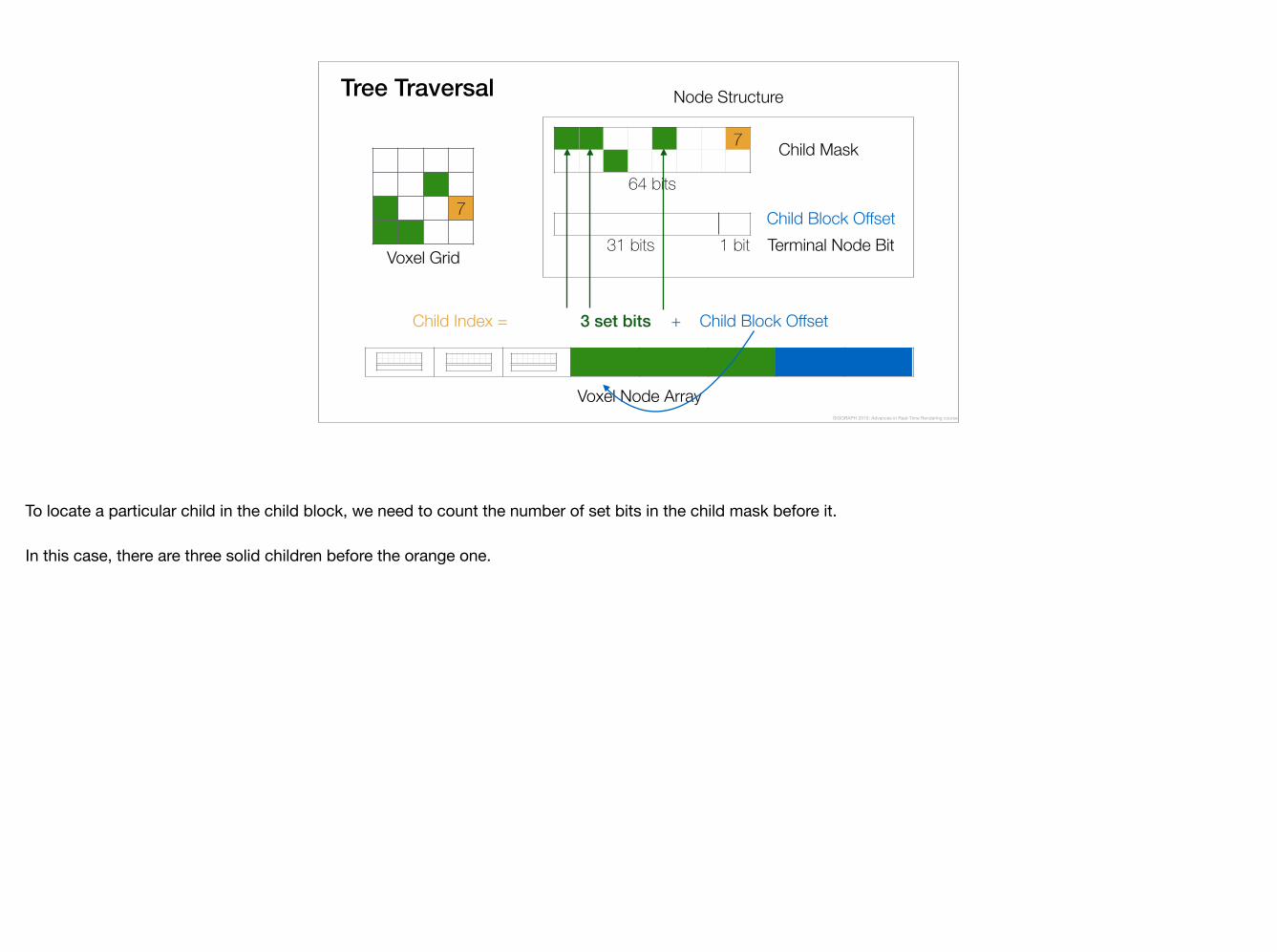
To locate a particular child in the child block, we need to count the number of set bits in the child mask before it.
In this case, there are three solid children before the orange one.
Voxel Node Array
7 Child Mask
Child Block Offset
64 bits
31 bits Terminal Node Bit1 bit
7
Voxel Grid
Node StructureTree Traversal
+ Child Block Offset3 set bitsChild Index =
SIGGRAPH 2015: Advances in Real-Time Rendering course
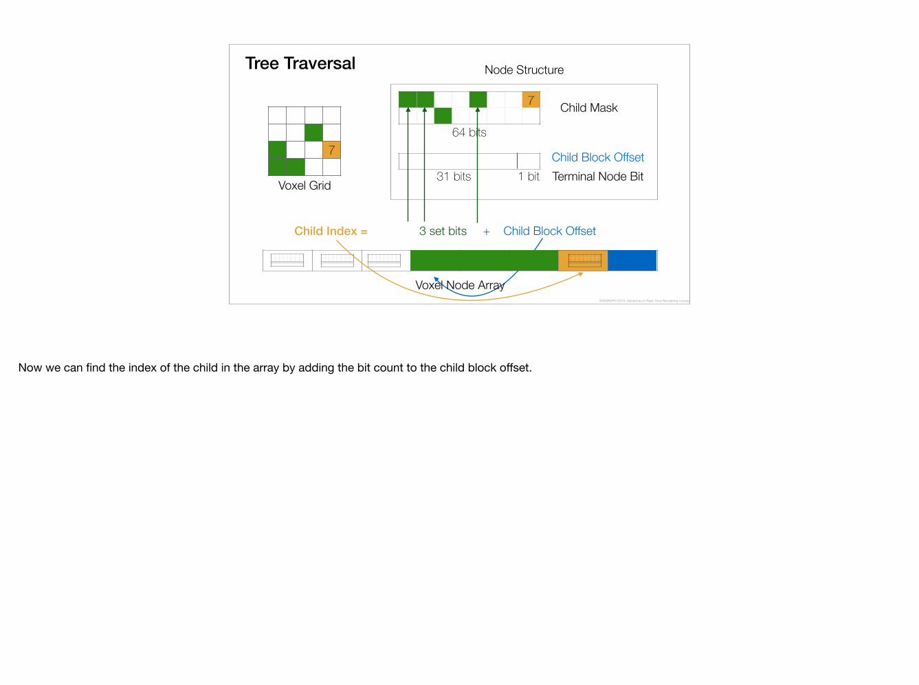
Now we can find the index of the child in the array by adding the bit count to the child block offset.
Voxel Node Array
7 Child Mask
Child Block Offset
64 bits
31 bits Terminal Node Bit1 bit
7
Voxel Grid
Node StructurePayload Data
+ Child Block Offset3 set bitsPayload Index = Child Index =
SIGGRAPH 2015: Advances in Real-Time Rendering course
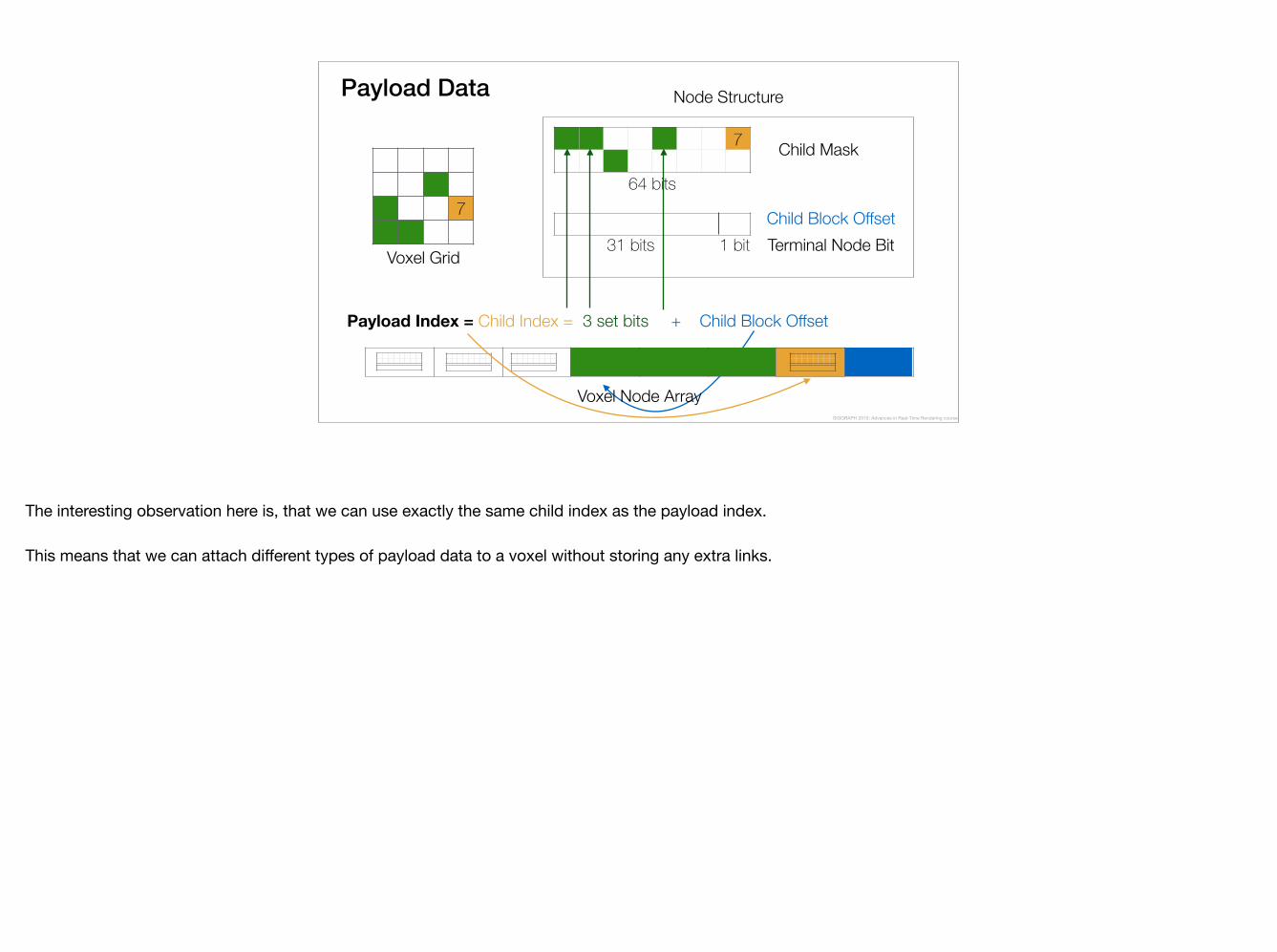
The interesting observation here is, that we can use exactly the same child index as the payload index.
This means that we can attach different types of payload data to a voxel without storing any extra links.

Payload Data
Voxel Node Array
Local Light Irradiance
Indirect Sun Light Transport
Sky Light Transport
Specular Probe Visibility
SIGGRAPH 2015: Advances in Real-Time Rendering course
For example, we store the light transport matrices, local light irradiance and specular probe visibility in the payload arrays.
Furthermore, it is easy to add or remove payload data without modifying the tree structure.

What About Leaf Nodes?
Leaf nodes are implicit: they only show up in the child masks of their parent voxels
Compact trees encoding only the topology
Only a few hundred kilobytes for an entire level
SIGGRAPH 2015: Advances in Real-Time Rendering course
It is worth noting that the leaf nodes are not explicitly stored anywhere: they are fully described by the child mask of their parent nodes.
The implicit encoding of the payload indices lead to compact trees, which take only a few hundred kilobytes per level.

First Level Lookup
First level of the tree can have arbitrary dimensions
We use a dense grid of 8x8x8 meter cells to guarantee coverage for large dynamic objects
SIGGRAPH 2015: Advances in Real-Time Rendering course
Similar to OpenVDB, the first level of the tree can have arbitrary dimensions. Instead of using a spatial hash, we store the first level of the tree in a dense lookup grid.
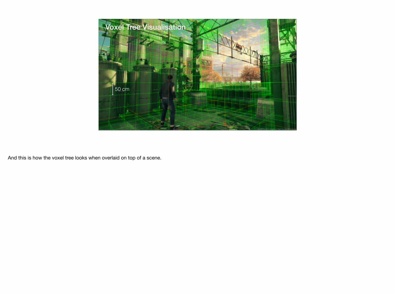
Voxel Tree Visualisation
50 cm
SIGGRAPH 2015: Advances in Real-Time Rendering course
And this is how the voxel tree looks when overlaid on top of a scene.

Seamless Interpolation
Dynamic and static objects lit by same data Need seamless interpolation everywhere
SIGGRAPH 2015: Advances in Real-Time Rendering course
We use the same GI data to light both dynamic and static objects, and this is the key to achieving a consistent look across the board.
I’ll skip the details for brevity, but you can find more information in the downloadable slides.
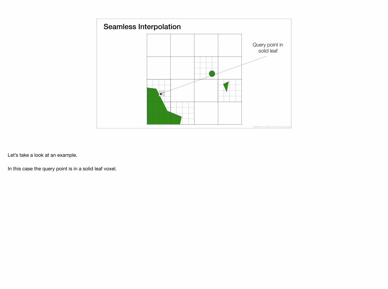
Seamless Interpolation
Query point in solid leaf
SIGGRAPH 2015: Advances in Real-Time Rendering course
Let’s take a look at an example.
In this case the query point is in a solid leaf voxel.
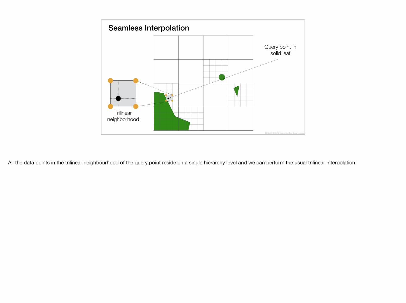
Seamless Interpolation
Trilinear neighborhood
Query point in solid leaf
SIGGRAPH 2015: Advances in Real-Time Rendering course
All the data points in the trilinear neighbourhood of the query point reside on a single hierarchy level and we can perform the usual trilinear interpolation.

Seamless Interpolation
Query point in empty leaf
SIGGRAPH 2015: Advances in Real-Time Rendering course
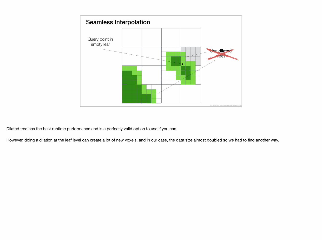
However, the general case, when query point is in an empty leaf, is more interesting.
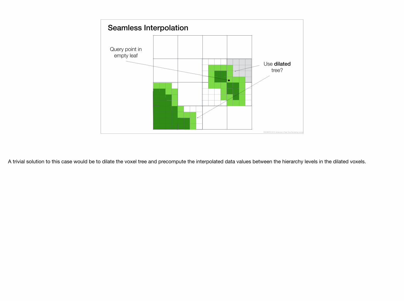
Seamless Interpolation
Query point in empty leaf
Use dilated tree?
SIGGRAPH 2015: Advances in Real-Time Rendering course
A trivial solution to this case would be to dilate the voxel tree and precompute the interpolated data values between the hierarchy levels in the dilated voxels.
Seamless Interpolation
Query point in empty leaf
Use dilated tree?
SIGGRAPH 2015: Advances in Real-Time Rendering course
Dilated tree has the best runtime performance and is a perfectly valid option to use if you can.
However, doing a dilation at the leaf level can create a lot of new voxels, and in our case, the data size almost doubled so we had to find another way.
Seamless Interpolation
Query point in empty leaf
Trilinear neighborhood
?
SIGGRAPH 2015: Advances in Real-Time Rendering course
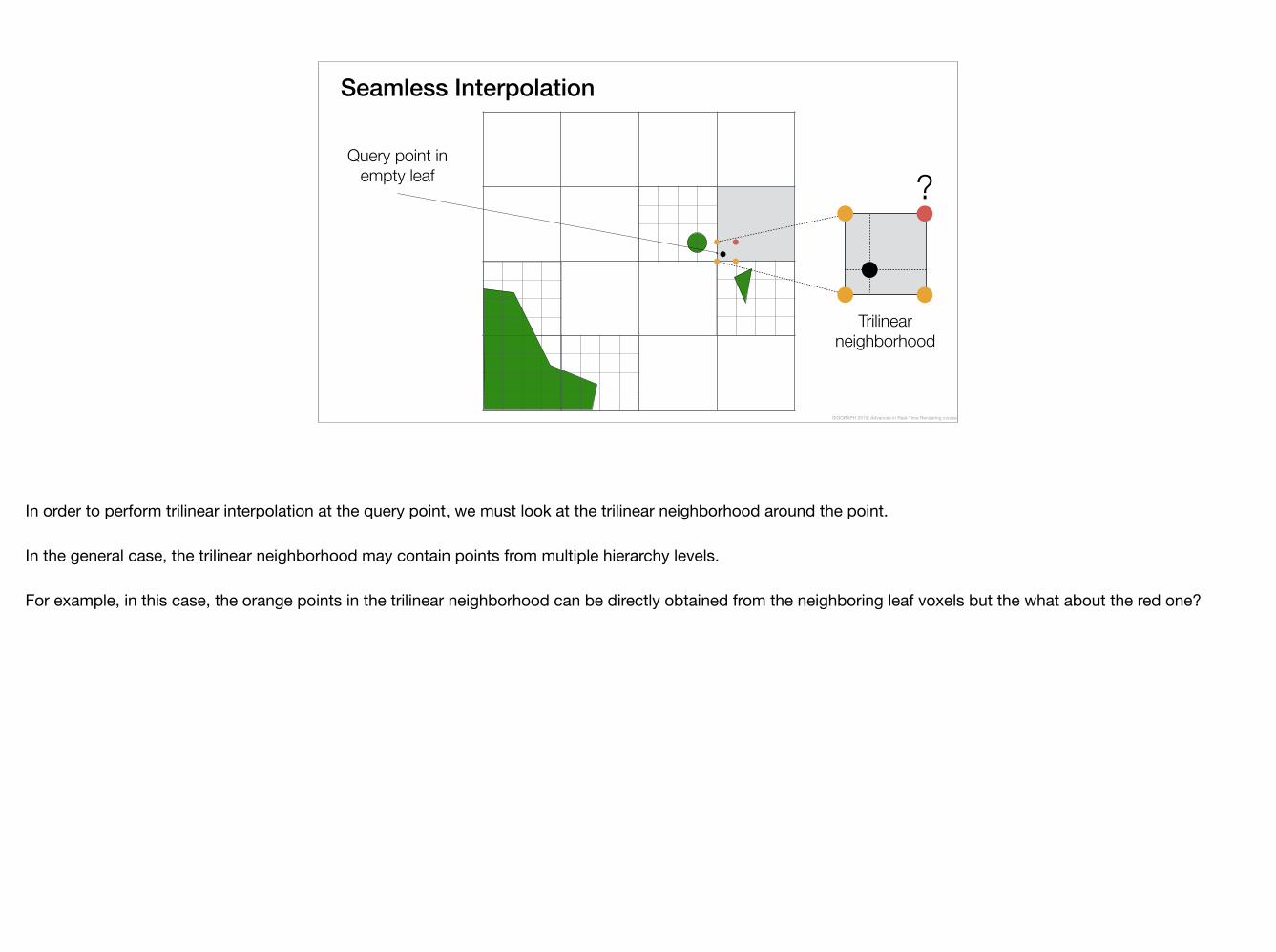
In order to perform trilinear interpolation at the query point, we must look at the trilinear neighborhood around the point.
In the general case, the trilinear neighborhood may contain points from multiple hierarchy levels.
For example, in this case, the orange points in the trilinear neighborhood can be directly obtained from the neighboring leaf voxels but the what about the red one?
Seamless Interpolation
Query point in empty leaf
Trilinear neighborhood
Interpolate from parent node
SIGGRAPH 2015: Advances in Real-Time Rendering course
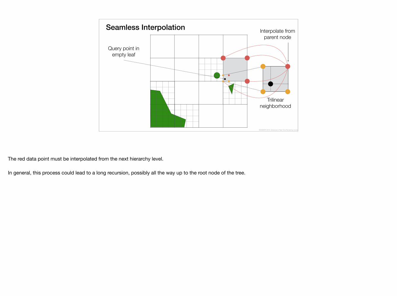
The red data point must be interpolated from the next hierarchy level.
In general, this process could lead to a long recursion, possibly all the way up to the root node of the tree.
Seamless Interpolation
Query point in empty leaf
Trilinear neighborhood
Apply partial dilation to avoid recursion
Interpolate from parent node
SIGGRAPH 2015: Advances in Real-Time Rendering course
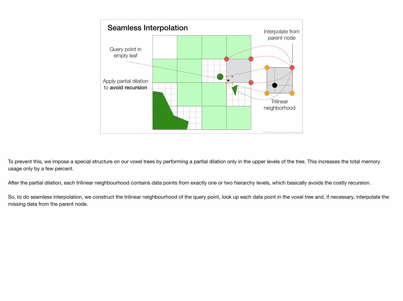
To prevent this, we impose a special structure on our voxel trees by performing a partial dilation only in the upper levels of the tree. This increases the total memory usage only by a few percent.
After the partial dilation, each trilinear neighbourhood contains data points from exactly one or two hierarchy levels, which basically avoids the costly recursion.
So, to do seamless interpolation, we construct the trilinear neighbourhood of the query point, look up each data point in the voxel tree and, if necessary, interpolate the missing data from the parent node.

Seamless InterpolationSeamless Interpolation
0.5m voxels 2m voxels8m voxels
SIGGRAPH 2015: Advances in Real-Time Rendering course
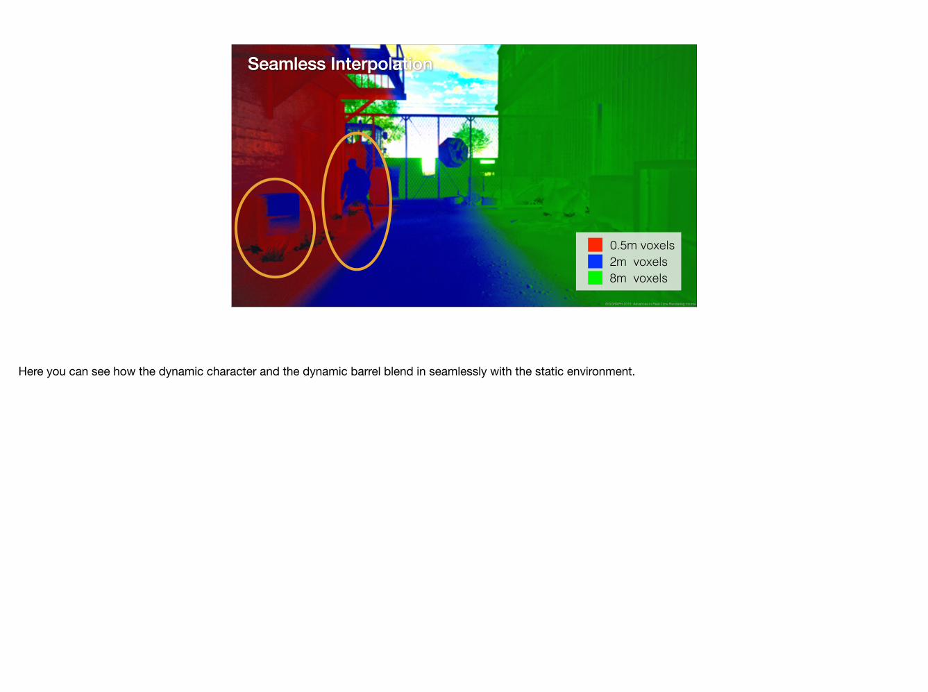
And this is how the seamless interpolation looks in game.
Seamless InterpolationSeamless Interpolation
0.5m voxels 2m voxels8m voxels
SIGGRAPH 2015: Advances in Real-Time Rendering course
Here you can see how the dynamic character and the dynamic barrel blend in seamlessly with the static environment.
Seamless InterpolationSeamless Interpolation
0.5m voxels 2m voxels8m voxels
SIGGRAPH 2015: Advances in Real-Time Rendering course
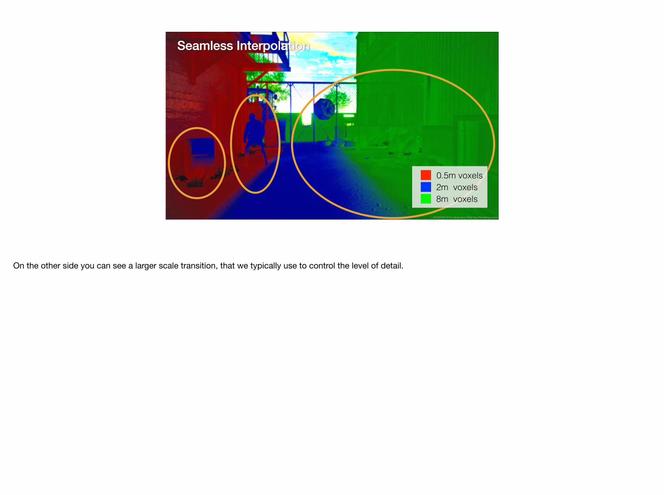
On the other side you can see a larger scale transition, that we typically use to control the level of detail.
Seamless InterpolationSeamless Interpolation
SIGGRAPH 2015: Advances in Real-Time Rendering course
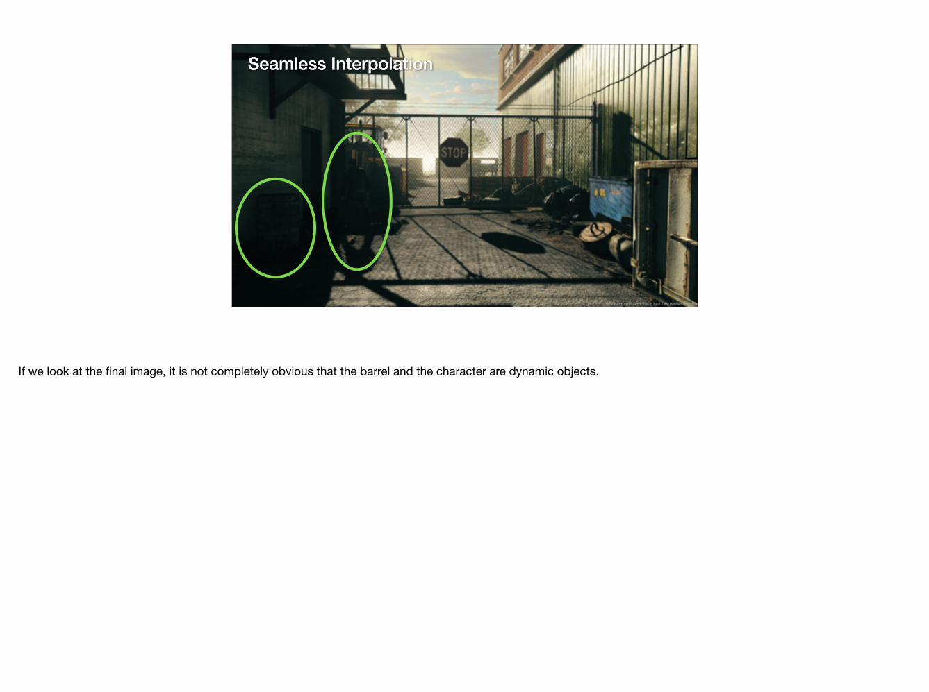
If we look at the final image, it is not completely obvious that the barrel and the character are dynamic objects.
Geometry Weights
✓n
l
Multiply trilinear weight with
On
Off
max(0, cos ✓)
SIGGRAPH 2015: Advances in Real-Time Rendering course
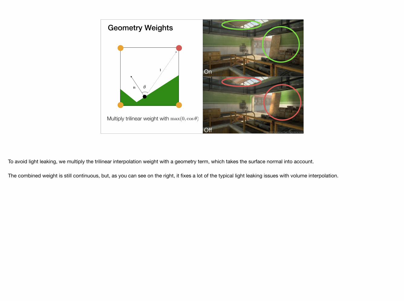
To avoid light leaking, we multiply the trilinear interpolation weight with a geometry term, which takes the surface normal into account.
The combined weight is still continuous, but, as you can see on the right, it fixes a lot of the typical light leaking issues with volume interpolation.

Scaling to Large Scenes
World is divided into a cell grid for streaming
Per cell voxel tree
World Atlas
128 m
128 m
SIGGRAPH 2015: Advances in Real-Time Rendering course
So far we have talked about a single voxel tree structure.
In order to support large levels and streaming, we divide the world space into 128-by-128 meter cells.
Each world space cell contains it own voxel tree and a full set of GI data.
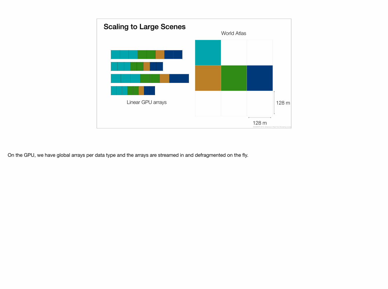
Scaling to Large Scenes
Linear GPU arrays
World Atlas
128 m
128 m
SIGGRAPH 2015: Advances in Real-Time Rendering course
On the GPU, we have global arrays per data type and the arrays are streamed in and defragmented on the fly.
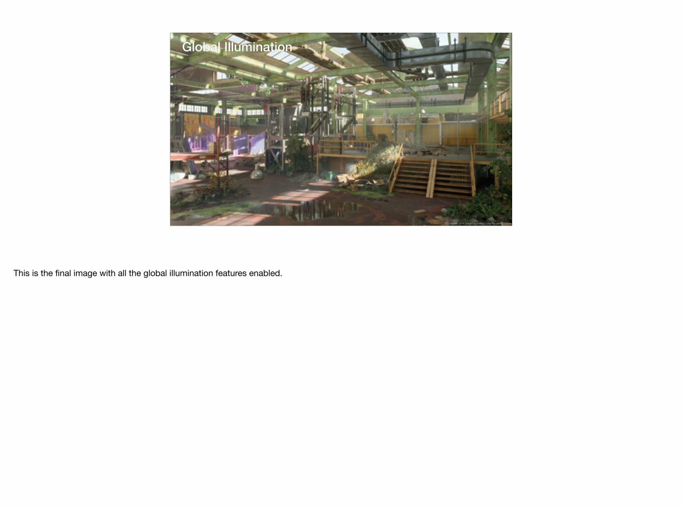
Global Illumination
SIGGRAPH 2015: Advances in Real-Time Rendering course
This is the final image with all the global illumination features enabled.
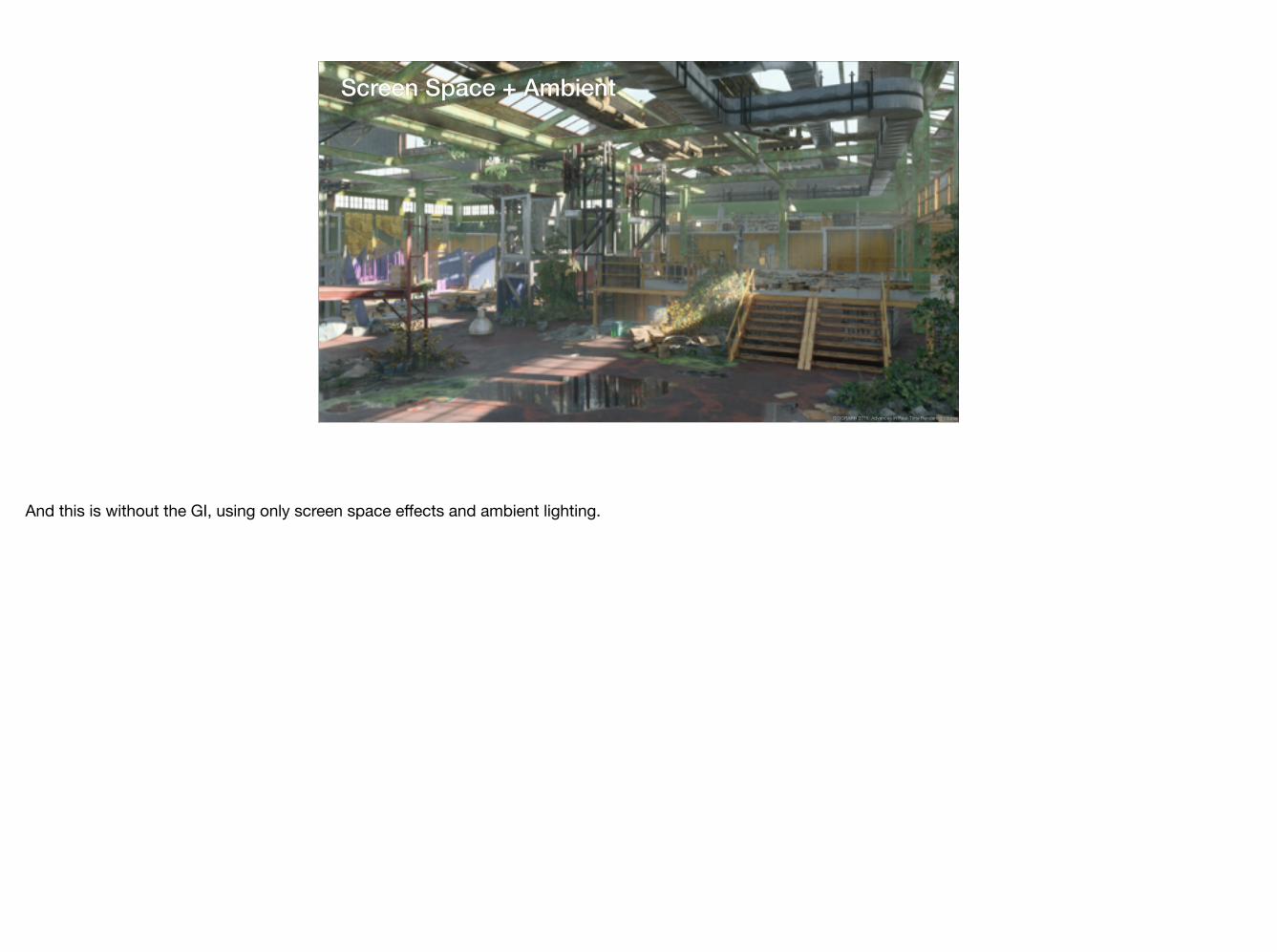
Screen Space + Ambient
SIGGRAPH 2015: Advances in Real-Time Rendering course
And this is without the GI, using only screen space effects and ambient lighting.
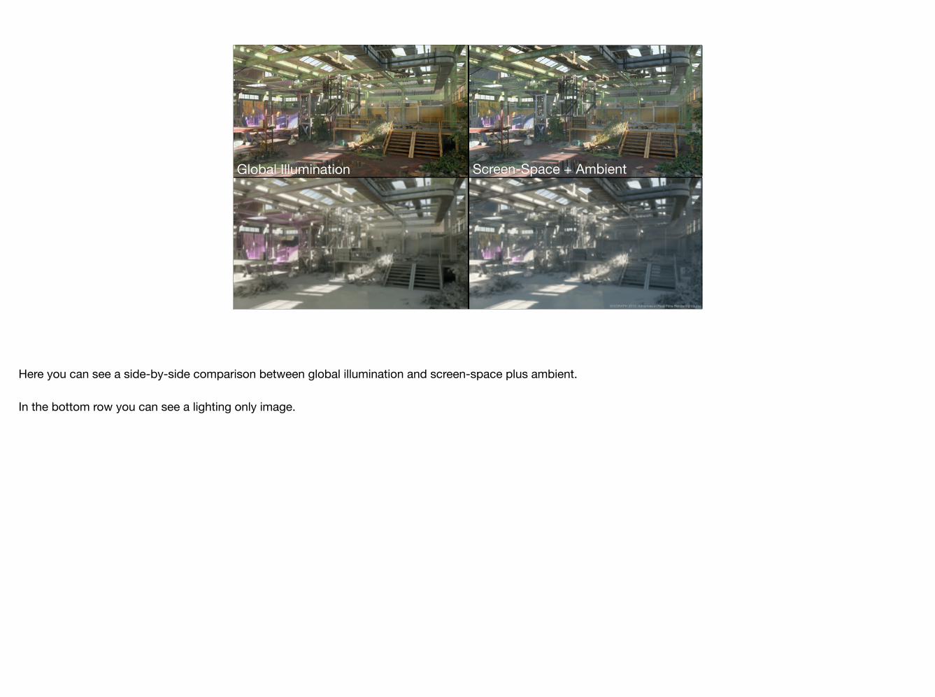
ON OFFGlobal Illumination Screen-Space + Ambient
SIGGRAPH 2015: Advances in Real-Time Rendering course
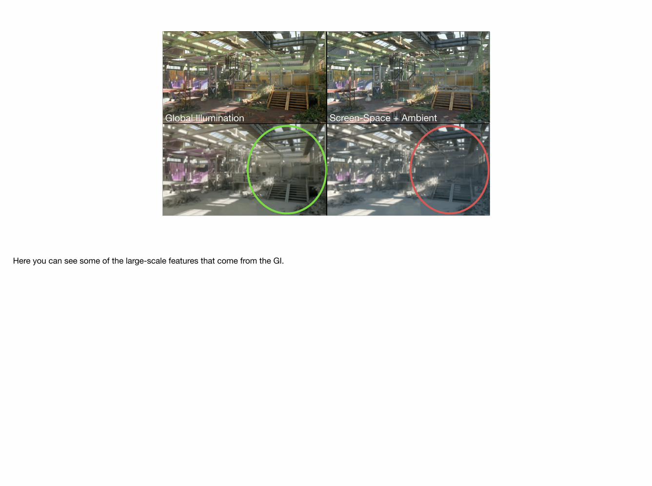
Here you can see a side-by-side comparison between global illumination and screen-space plus ambient.
In the bottom row you can see a lighting only image.
ON OFFGlobal Illumination Screen-Space + Ambient
Here you can see some of the large-scale features that come from the GI.
Performance
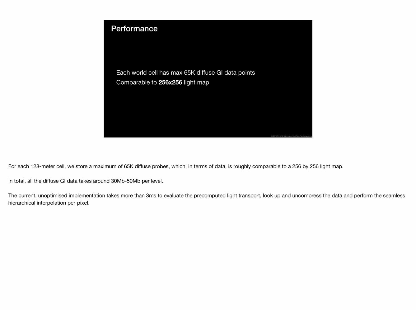
Each world cell has max 65K diffuse GI data pointsComparable to 256x256 light map
SIGGRAPH 2015: Advances in Real-Time Rendering course
For each 128-meter cell, we store a maximum of 65K diffuse probes, which, in terms of data, is roughly comparable to a 256 by 256 light map.
In total, all the diffuse GI data takes around 30Mb-50Mb per level.
The current, unoptimised implementation takes more than 3ms to evaluate the precomputed light transport, look up and uncompress the data and perform the seamless hierarchical interpolation per-pixel.
Performance
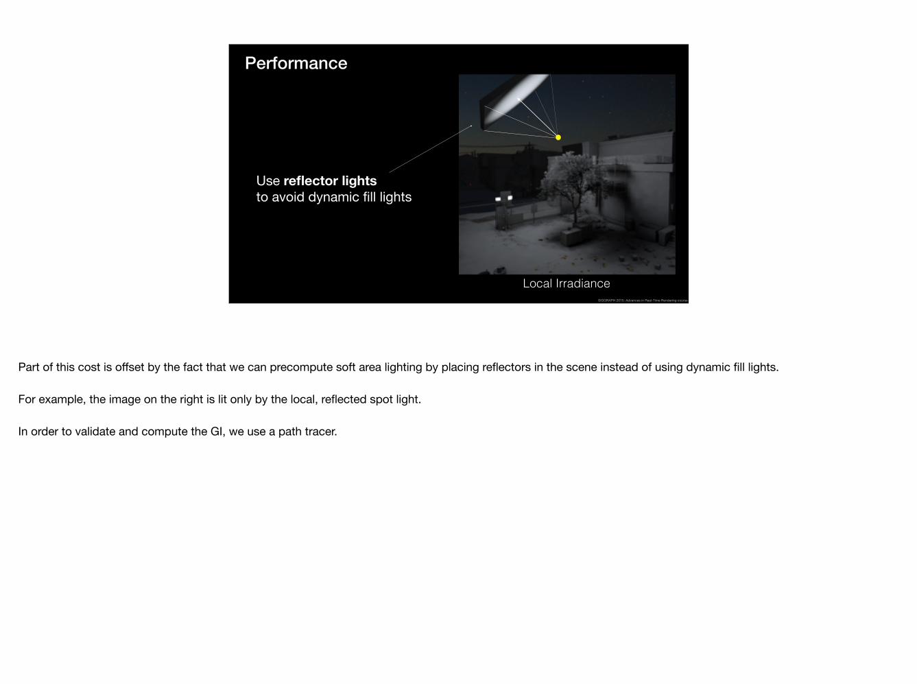
Use reflector lights to avoid dynamic fill lights
Local IrradianceSIGGRAPH 2015: Advances in Real-Time Rendering course
Part of this cost is offset by the fact that we can precompute soft area lighting by placing reflectors in the scene instead of using dynamic fill lights.
For example, the image on the right is lit only by the local, reflected spot light.
In order to validate and compute the GI, we use a path tracer.
Real-Time Indirect
Direct Only Global Illumination
Reference Indirect
Direct Only
Reference Indirect Real-Time Indirect
Global Illumination
SIGGRAPH 2015: Advances in Real-Time Rendering course
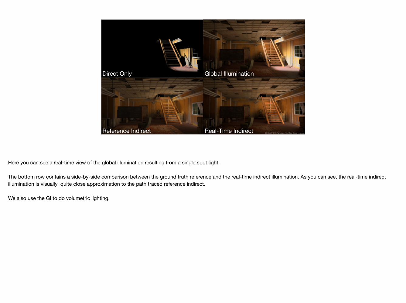
Here you can see a real-time view of the global illumination resulting from a single spot light.
The bottom row contains a side-by-side comparison between the ground truth reference and the real-time indirect illumination. As you can see, the real-time indirect illumination is visually quite close approximation to the path traced reference indirect.
We also use the GI to do volumetric lighting.
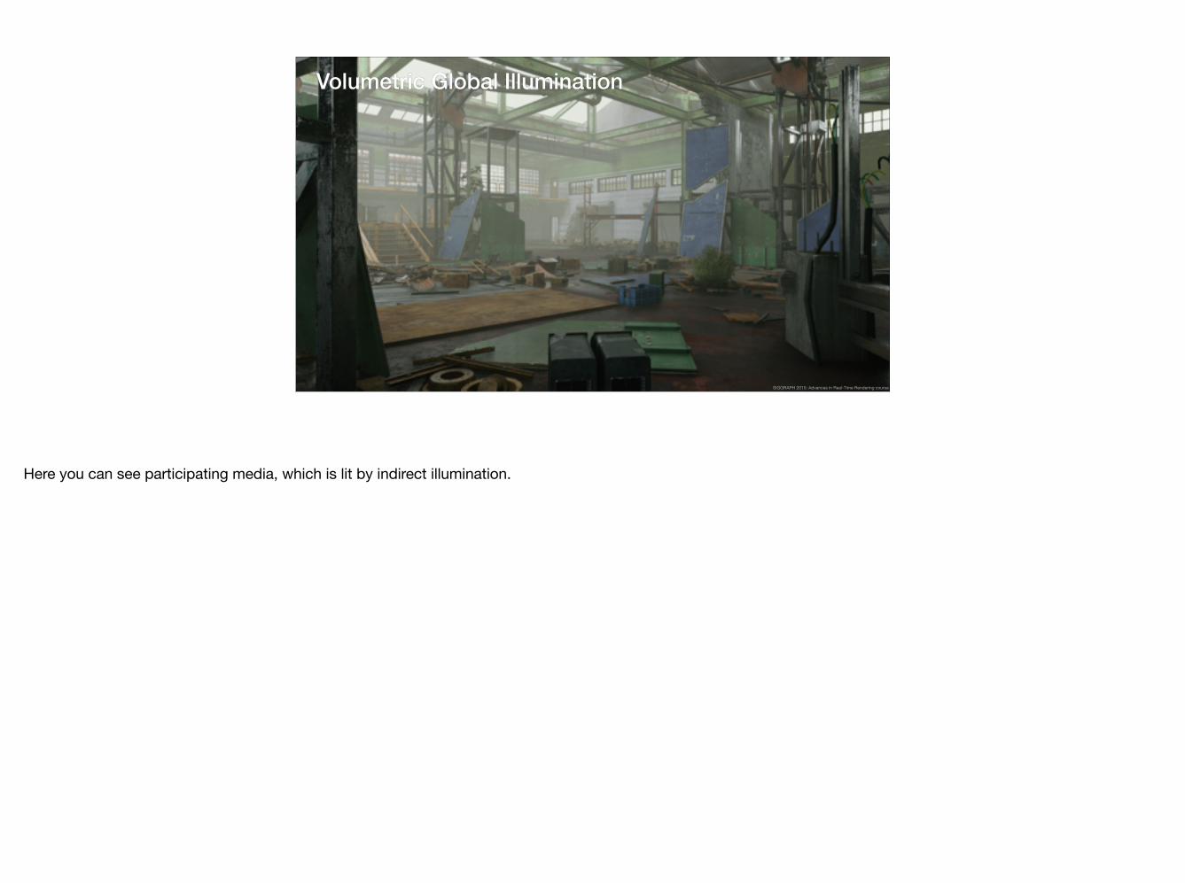
Volumetric Global Illumination
SIGGRAPH 2015: Advances in Real-Time Rendering course
Here you can see participating media, which is lit by indirect illumination.
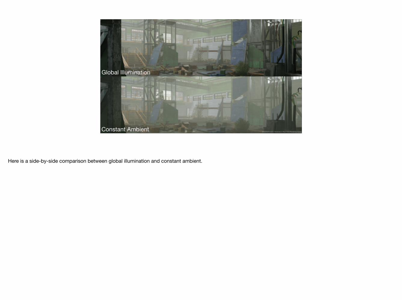
Global Illumination
Constant Ambient SIGGRAPH 2015: Advances in Real-Time Rendering course
Here is a side-by-side comparison between global illumination and constant ambient.

Constant Ambient
Global Illumination
SIGGRAPH 2015: Advances in Real-Time Rendering course
Here you can see how the volumetric GI makes the image work better.
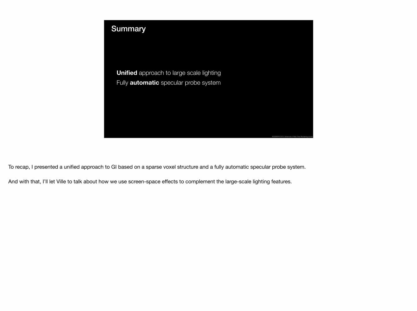
Summary
Unified approach to large scale lighting Fully automatic specular probe system
SIGGRAPH 2015: Advances in Real-Time Rendering course
To recap, I presented a unified approach to GI based on a sparse voxel structure and a fully automatic specular probe system.
And with that, I’ll let Ville to talk about how we use screen-space effects to complement the large-scale lighting features.
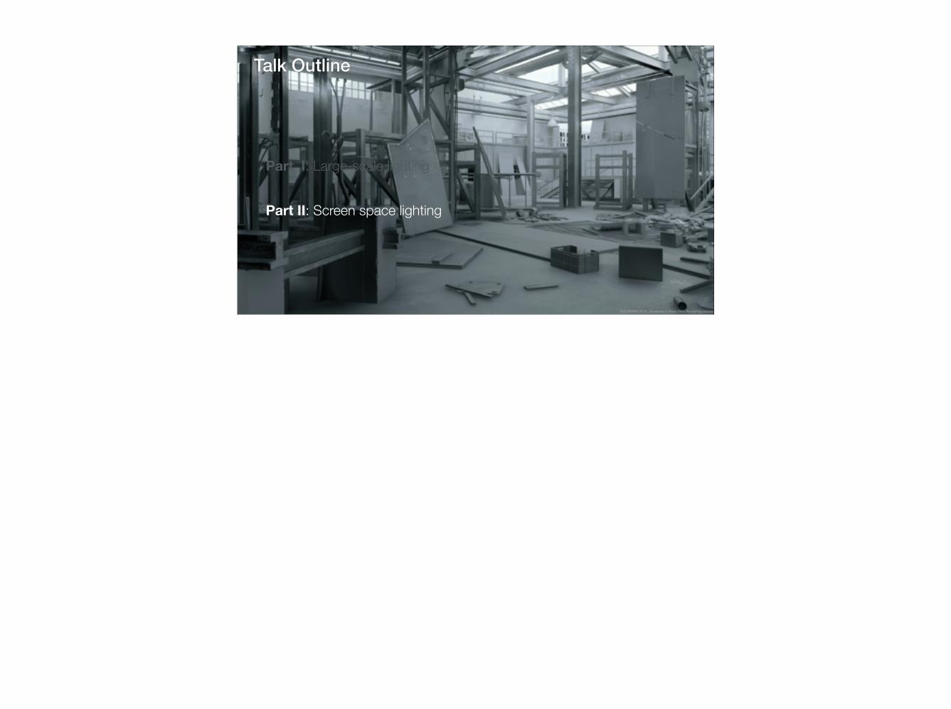
Talk Outline
Part I: Large-scale lighting
Part II: Screen space lighting
SIGGRAPH 2015: Advances in Real-Time Rendering course
Screen-Space Techniques
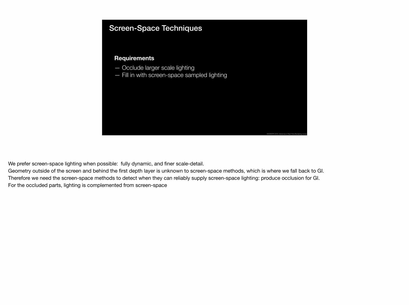
Requirements — Occlude larger scale lighting — Fill in with screen-space sampled lighting
SIGGRAPH 2015: Advances in Real-Time Rendering course
We prefer screen-space lighting when possible: fully dynamic, and finer scale-detail.Geometry outside of the screen and behind the first depth layer is unknown to screen-space methods, which is where we fall back to GI.Therefore we need the screen-space methods to detect when they can reliably supply screen-space lighting: produce occlusion for GI.For the occluded parts, lighting is complemented from screen-space
Screen-Space Ambient Occlusion and Diffuse
SIGGRAPH 2015: Advances in Real-Time Rendering course
We treat diffuse and specular separately, and first present our diffuse solution.
GI diffuse occlusion Screen-Space DiffuseSIGGRAPH 2015: Advances in Real-Time Rendering course
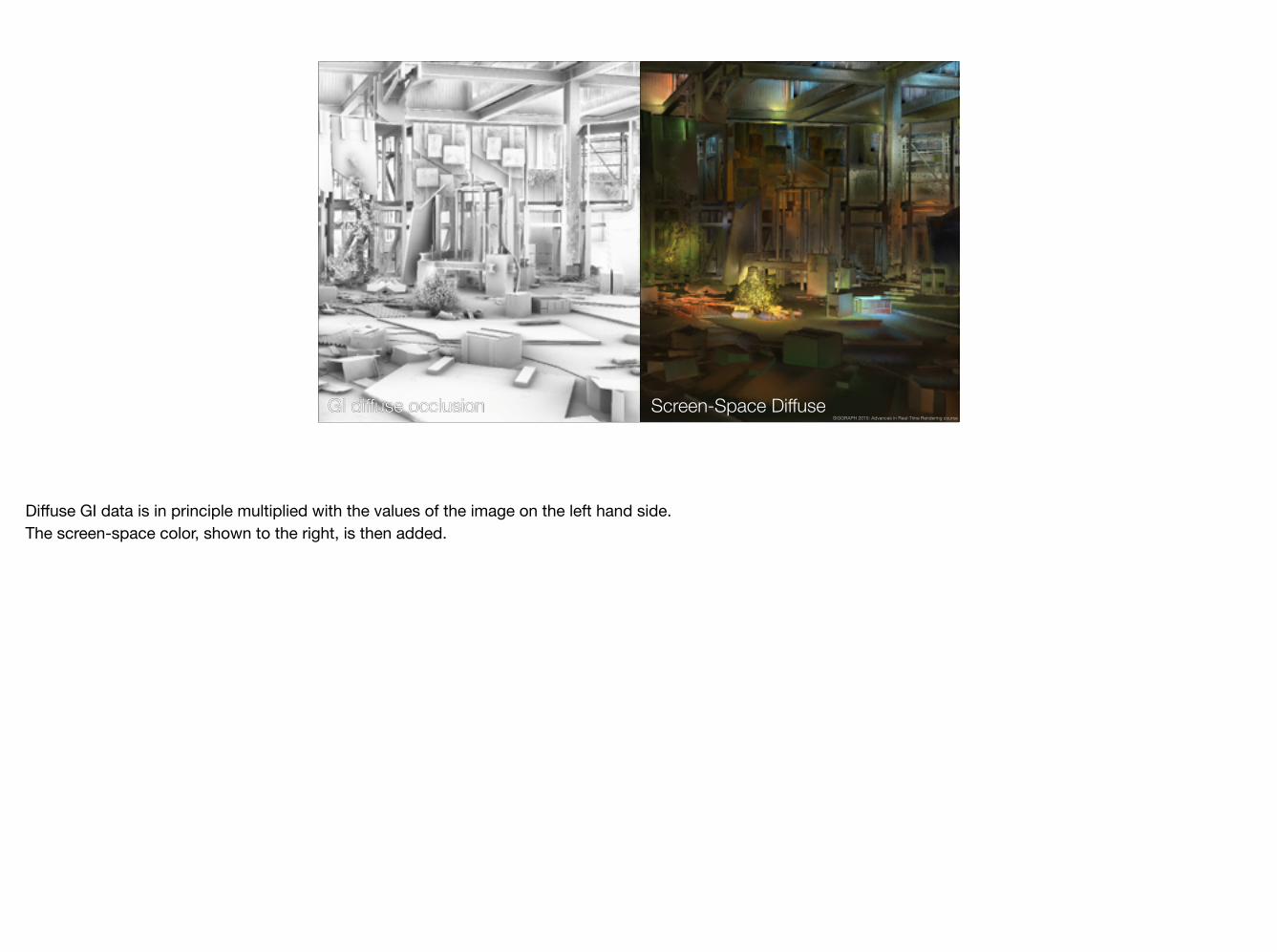
Diffuse GI data is in principle multiplied with the values of the image on the left hand side.The screen-space color, shown to the right, is then added.
Screen-Space Ambient Occlusion
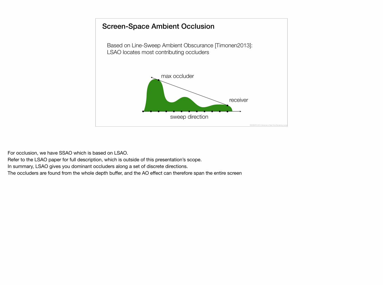
Based on Line-Sweep Ambient Obscurance [Timonen2013]: LSAO locates most contributing occluders
sweep direction
receiver
max occluder
SIGGRAPH 2015: Advances in Real-Time Rendering course
For occlusion, we have SSAO which is based on LSAO.Refer to the LSAO paper for full description, which is outside of this presentation’s scope.In summary, LSAO gives you dominant occluders along a set of discrete directions.The occluders are found from the whole depth buffer, and the AO effect can therefore span the entire screen

Screen-Space Ambient Occlusion
We scan in 36 directions, long steps (~10px) and short line spacing (~2px apart)— Scheduling friendly for the GPU — Scan is 0.75ms on Xbox One at 720p
SIGGRAPH 2015: Advances in Real-Time Rendering course
These are our LSAO settings. Despite the long steps, average distance to the nearest step is less than 3 px.
Screen-Space Ambient Occlusion
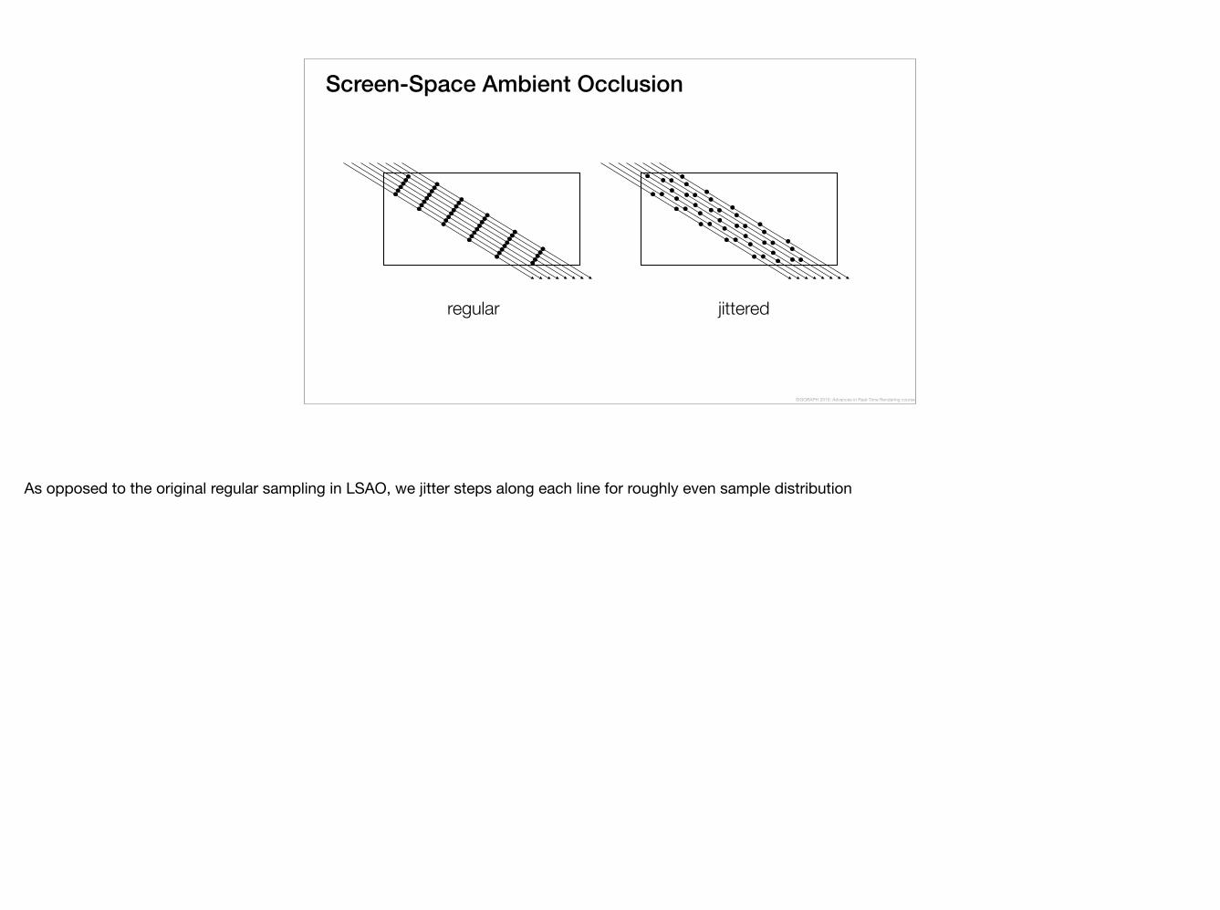
jitteredregular
SIGGRAPH 2015: Advances in Real-Time Rendering course
As opposed to the original regular sampling in LSAO, we jitter steps along each line for roughly even sample distribution

Screen-Space Ambient Occlusion
— An additional near field sample (at ~2px distance)— Sample normal to clamp occluders
receiver
near field sample
LSAO samples
SIGGRAPH 2015: Advances in Real-Time Rendering course
To fill in the “gaps” of the longer LSAO samples, we take one traditional near field sample per pixel per direction which is roughly half-way from the receiver to the nearest sample position of the sweep.
When we evaluate AO, we sample normal to clamp occluders to the visible hemisphere. This way we get AO that respects fine-scale normal variations.
Screen-Space Ambient Occlusion
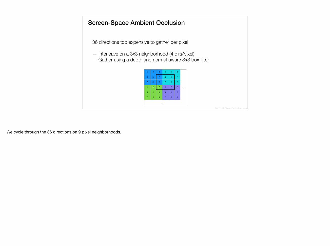
36 directions too expensive to gather per pixel— Interleave on a 3x3 neighborhood (4 dirs/pixel)— Gather using a depth and normal aware 3x3 box filter
1 2 3 1 2 3
…
4 5 6 4 5 6
7 8 9 7 8 9
1 2 3 1 2 3
4 5 6 4 5 6
7 8 9 7 8 9
…
SIGGRAPH 2015: Advances in Real-Time Rendering course
We cycle through the 36 directions on 9 pixel neighborhoods.
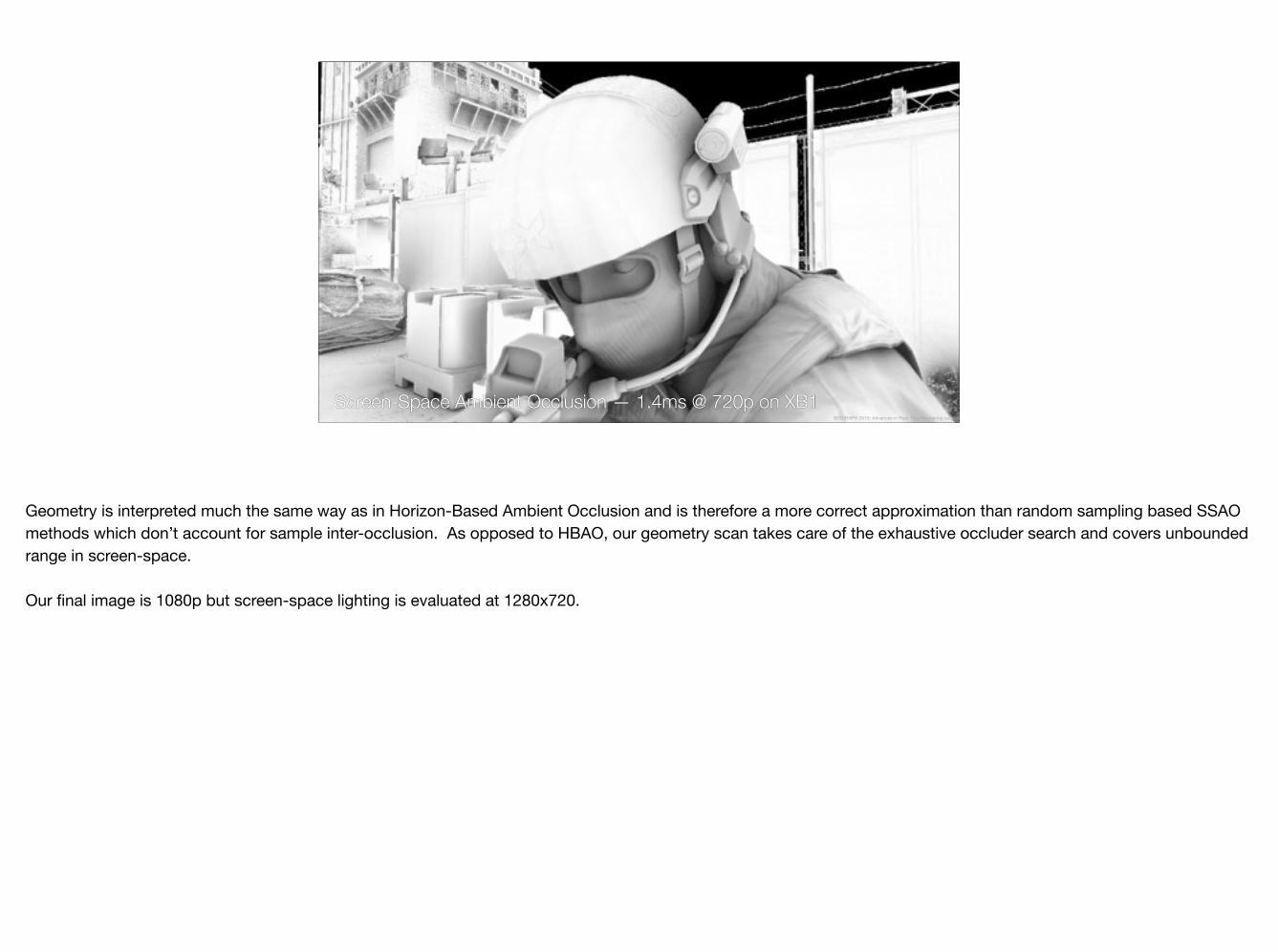
Screen-Space Ambient Occlusion — 1.4ms @ 720p on XB1SIGGRAPH 2015: Advances in Real-Time Rendering course
Geometry is interpreted much the same way as in Horizon-Based Ambient Occlusion and is therefore a more correct approximation than random sampling based SSAO methods which don’t account for sample inter-occlusion. As opposed to HBAO, our geometry scan takes care of the exhaustive occluder search and covers unbounded range in screen-space.
Our final image is 1080p but screen-space lighting is evaluated at 1280x720.
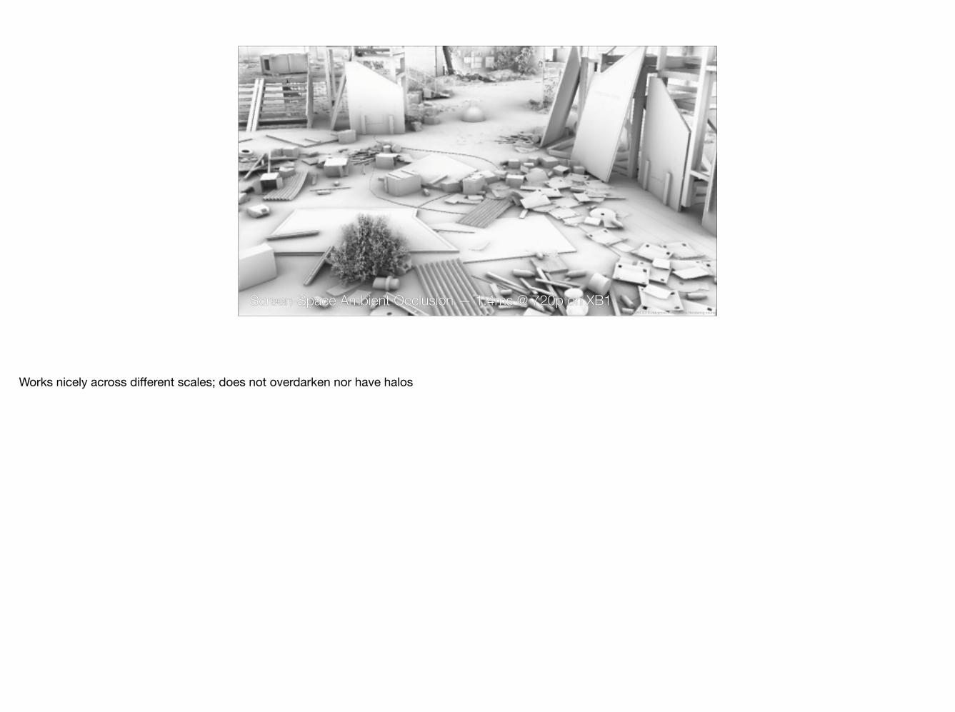
Screen-Space Ambient Occlusion 1.4ms @ 720pScreen-Space Ambient Occlusion — 1.4ms @ 720p on XB1SIGGRAPH 2015: Advances in Real-Time Rendering course
Works nicely across different scales; does not overdarken nor have halos
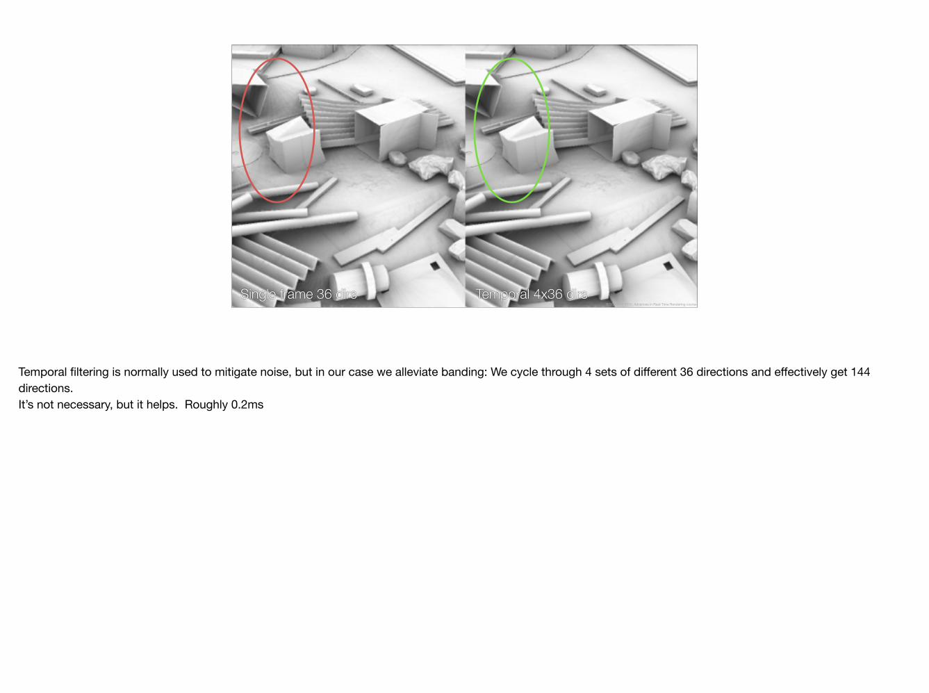
Temporal 4x36 dirsSingle frame 36 dirsSIGGRAPH 2015: Advances in Real-Time Rendering course
Temporal filtering is normally used to mitigate noise, but in our case we alleviate banding: We cycle through 4 sets of different 36 directions and effectively get 144 directions.It’s not necessary, but it helps. Roughly 0.2ms
Screen-Space Diffuse Lighting
SIGGRAPH 2015: Advances in Real-Time Rendering course
Now that the occlusion is covered, moving onto lighting
Screen-Space Diffuse Lighting
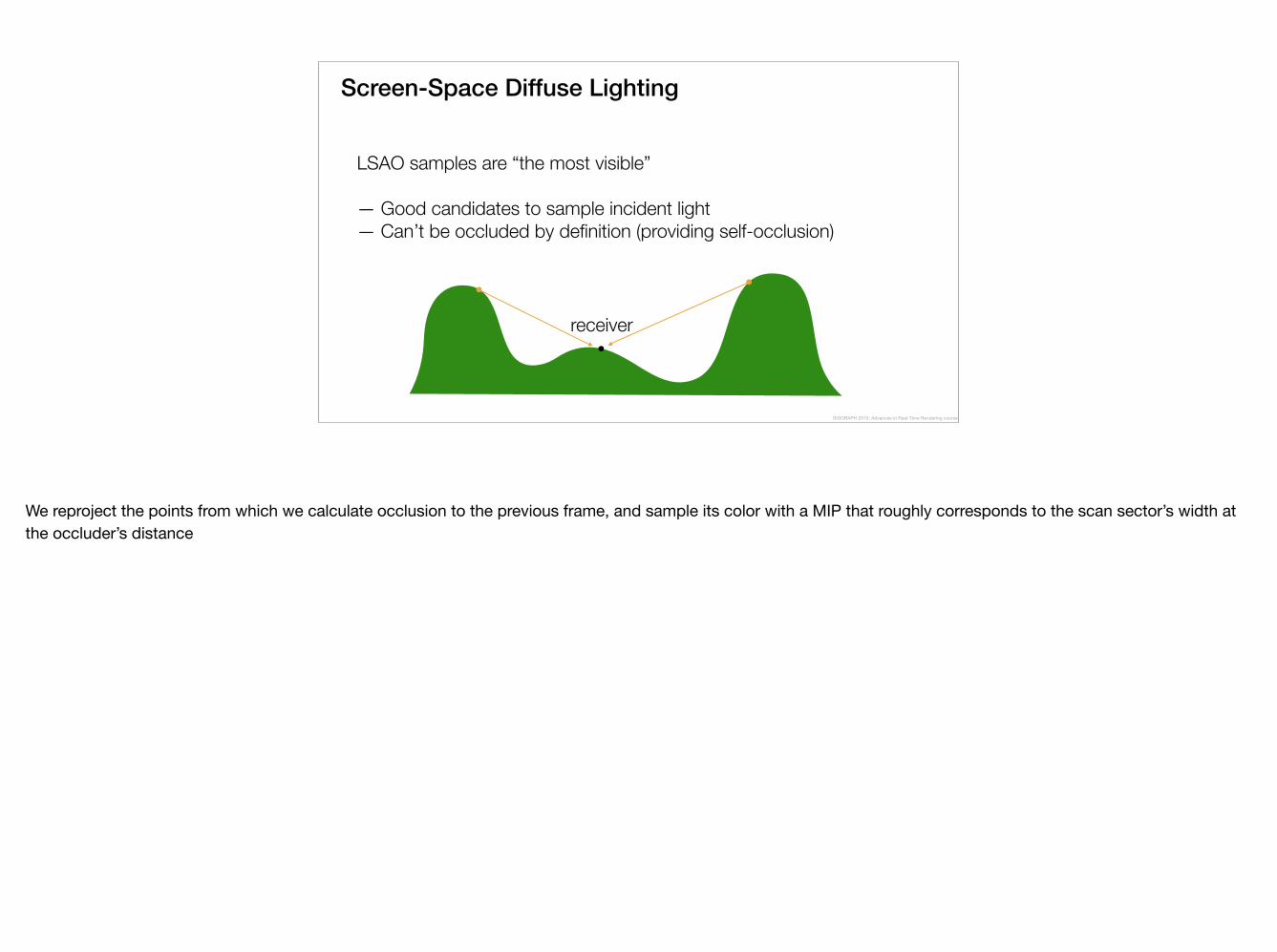
LSAO samples are “the most visible” — Good candidates to sample incident light— Can’t be occluded by definition (providing self-occlusion)
receiver
SIGGRAPH 2015: Advances in Real-Time Rendering course
We reproject the points from which we calculate occlusion to the previous frame, and sample its color with a MIP that roughly corresponds to the scan sector’s width at the occluder’s distance
Final imageScreen-Space Diffuse — 0.45msSIGGRAPH 2015: Advances in Real-Time Rendering course
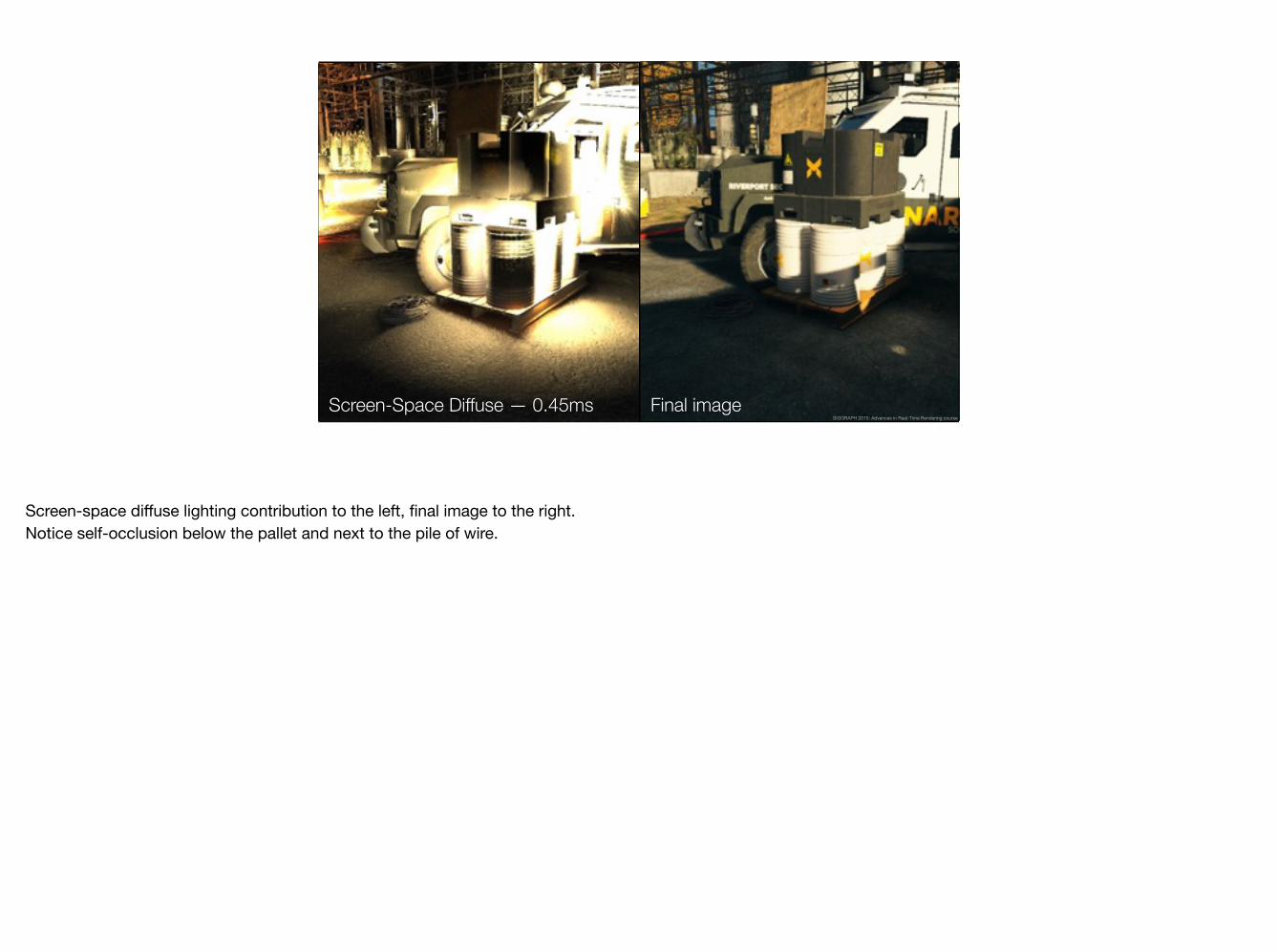
Screen-space diffuse lighting contribution to the left, final image to the right.Notice self-occlusion below the pallet and next to the pile of wire.
Screen-Space Ambient Occlusion 1.4ms @ 720p
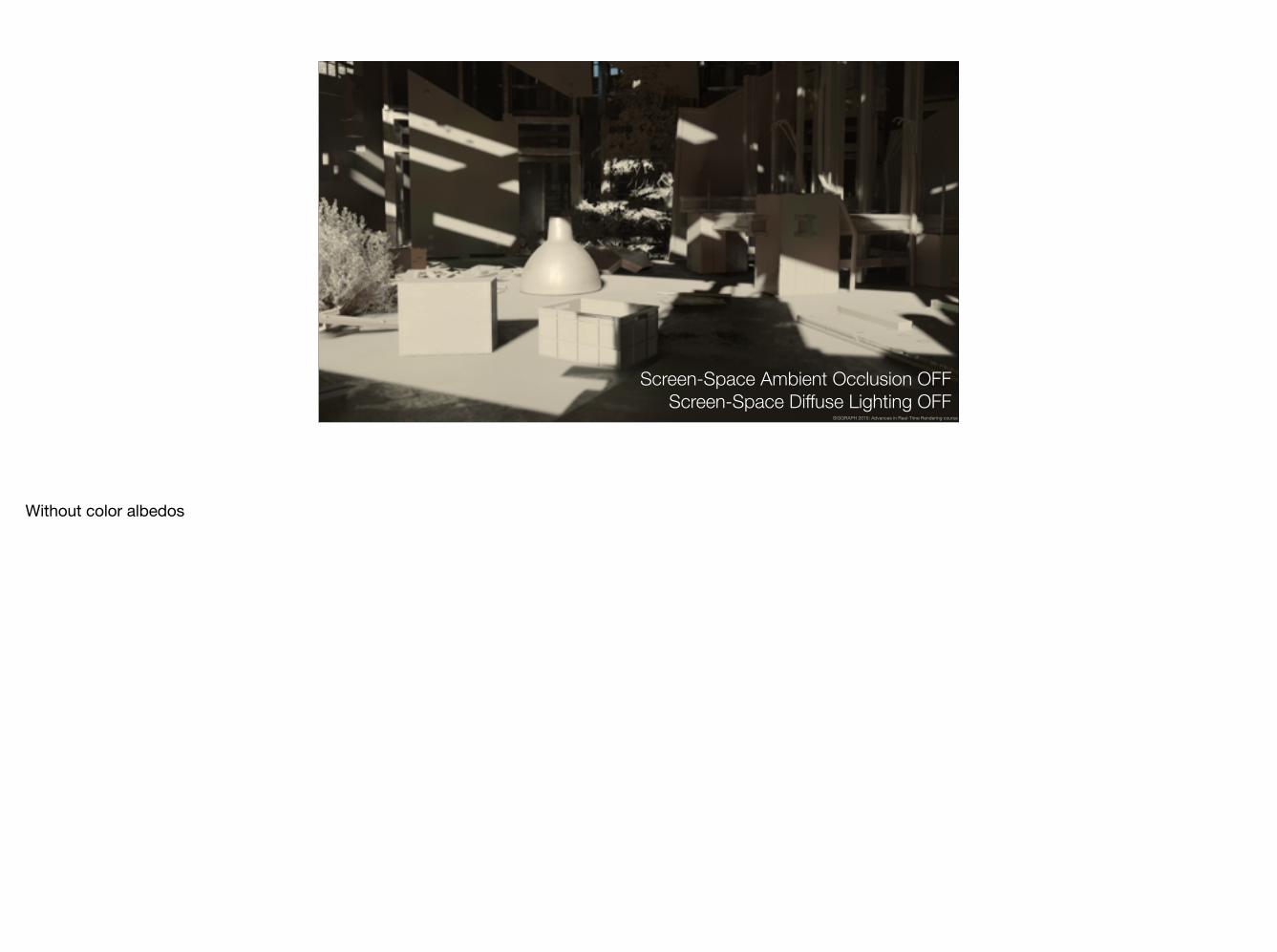
Screen-Space Ambient Occlusion OFFScreen-Space Diffuse Lighting OFF
SIGGRAPH 2015: Advances in Real-Time Rendering course
Without color albedos

Screen-Space Ambient Occlusion 1.4ms @ 720p
Screen-Space Ambient Occlusion ONScreen-Space Diffuse Lighting OFF
SIGGRAPH 2015: Advances in Real-Time Rendering course
Without color albedos

Screen-Space Ambient Occlusion 1.4ms @ 720p
Screen-Space Ambient Occlusion ONScreen-Space Diffuse Lighting ON
SIGGRAPH 2015: Advances in Real-Time Rendering course
Without color albedos
Screen-Space Ambient Occlusion 1.4ms @ 720p
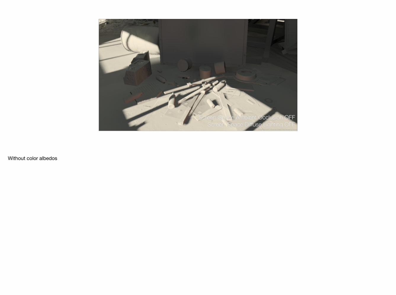
Screen-Space Ambient Occlusion OFFScreen-Space Diffuse Lighting OFF
SIGGRAPH 2015: Advances in Real-Time Rendering course
Without color albedos

Screen-Space Ambient Occlusion 1.4ms @ 720p
Screen-Space Ambient Occlusion ONScreen-Space Diffuse Lighting OFF
SIGGRAPH 2015: Advances in Real-Time Rendering course
Without color albedos

Screen-Space Ambient Occlusion 1.4ms @ 720p
Screen-Space Ambient Occlusion ONScreen-Space Diffuse Lighting ON
SIGGRAPH 2015: Advances in Real-Time Rendering course
Without color albedos
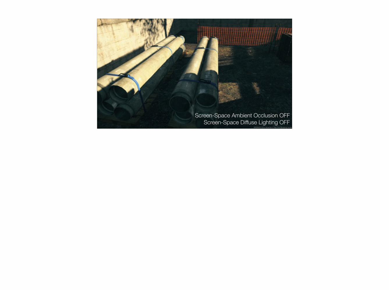
Screen-Space Ambient Occlusion OFFScreen-Space Diffuse Lighting OFF
SIGGRAPH 2015: Advances in Real-Time Rendering course
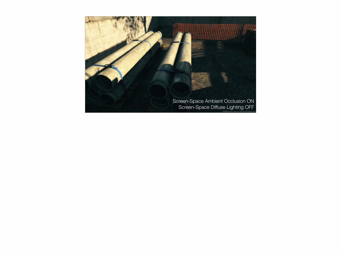
Screen-Space Ambient Occlusion ONScreen-Space Diffuse Lighting OFF
SIGGRAPH 2015: Advances in Real-Time Rendering course

Screen-Space Ambient Occlusion ONScreen-Space Diffuse Lighting ON
SIGGRAPH 2015: Advances in Real-Time Rendering course
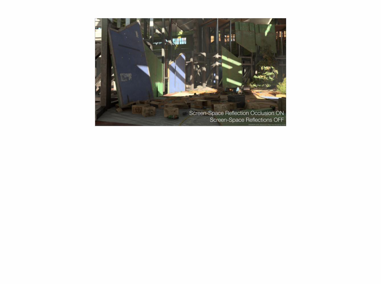
Screen-Space Reflections and Occlusion
SIGGRAPH 2015: Advances in Real-Time Rendering course
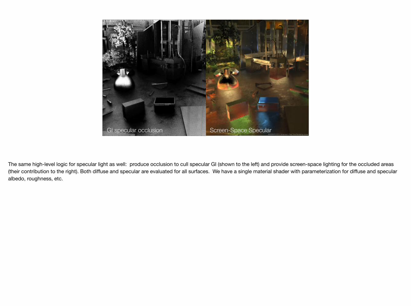
GI specular occlusion Screen-Space SpecularSIGGRAPH 2015: Advances in Real-Time Rendering course
The same high-level logic for specular light as well: produce occlusion to cull specular GI (shown to the left) and provide screen-space lighting for the occluded areas (their contribution to the right). Both diffuse and specular are evaluated for all surfaces. We have a single material shader with parameterization for diffuse and specular albedo, roughness, etc.
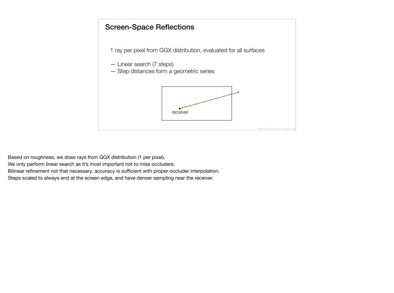
Screen-Space Reflections
1 ray per pixel from GGX distribution, evaluated for all surfaces — Linear search (7 steps)— Step distances form a geometric series
receiver
SIGGRAPH 2015: Advances in Real-Time Rendering course
Based on roughness, we draw rays from GGX distribution (1 per pixel).We only perform linear search as it’s most important not to miss occluders.Bilinear refinement not that necessary, accuracy is sufficient with proper occluder interpolation.Steps scaled to always end at the screen edge, and have denser sampling near the receiver.
Screen-Space Reflections
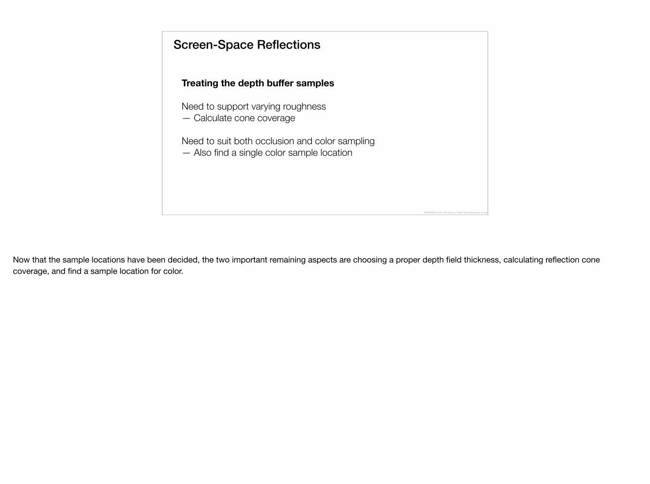
Treating the depth buffer samplesNeed to support varying roughness— Calculate cone coverageNeed to suit both occlusion and color sampling— Also find a single color sample location
SIGGRAPH 2015: Advances in Real-Time Rendering course
Now that the sample locations have been decided, the two important remaining aspects are choosing a proper depth field thickness, calculating reflection cone coverage, and find a sample location for color.
Screen-Space Reflections
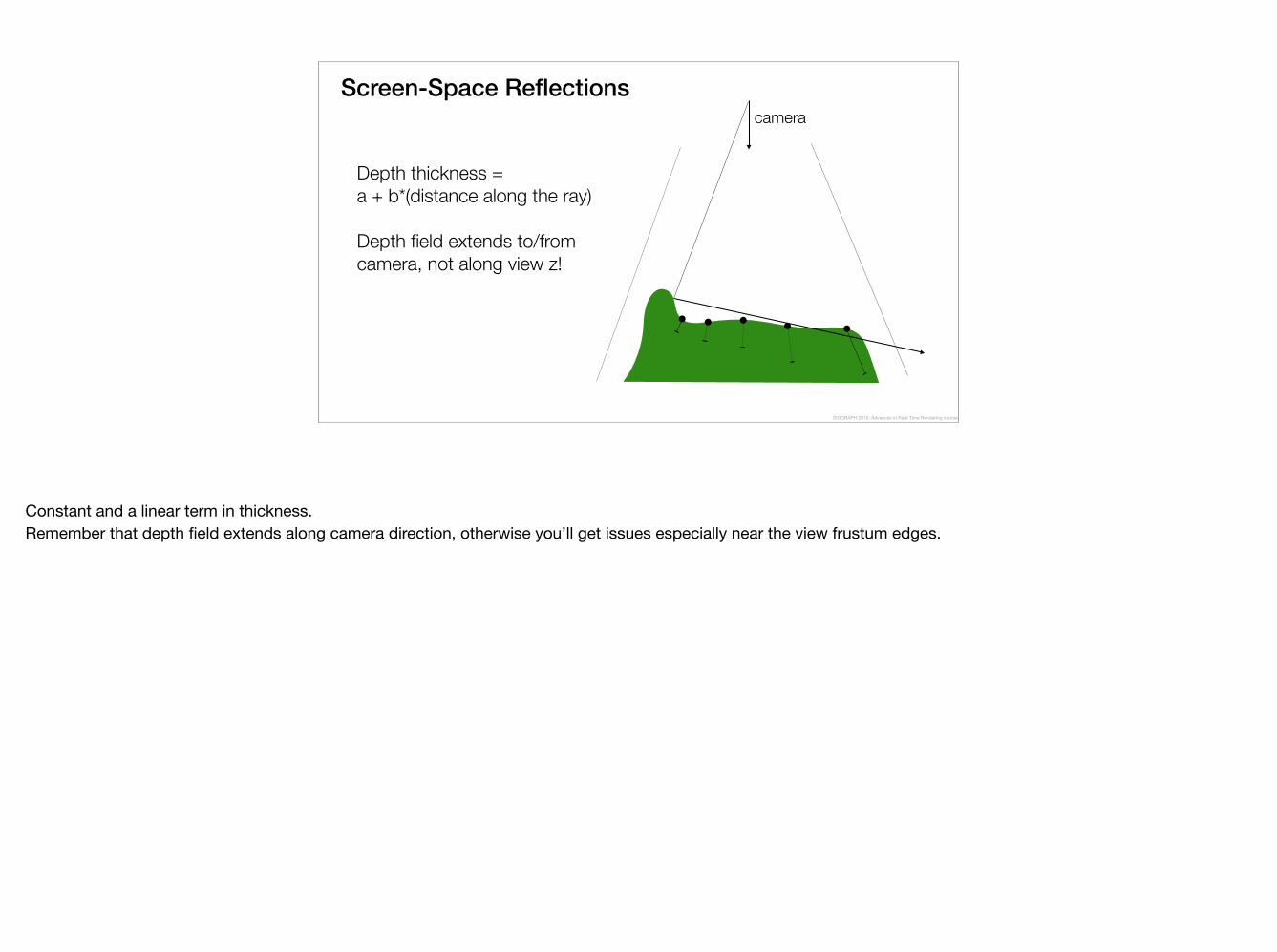
Depth thickness = a + b*(distance along the ray)Depth field extends to/from camera, not along view z!
camera
SIGGRAPH 2015: Advances in Real-Time Rendering course
Constant and a linear term in thickness.Remember that depth field extends along camera direction, otherwise you’ll get issues especially near the view frustum edges.
Screen-Space Reflections
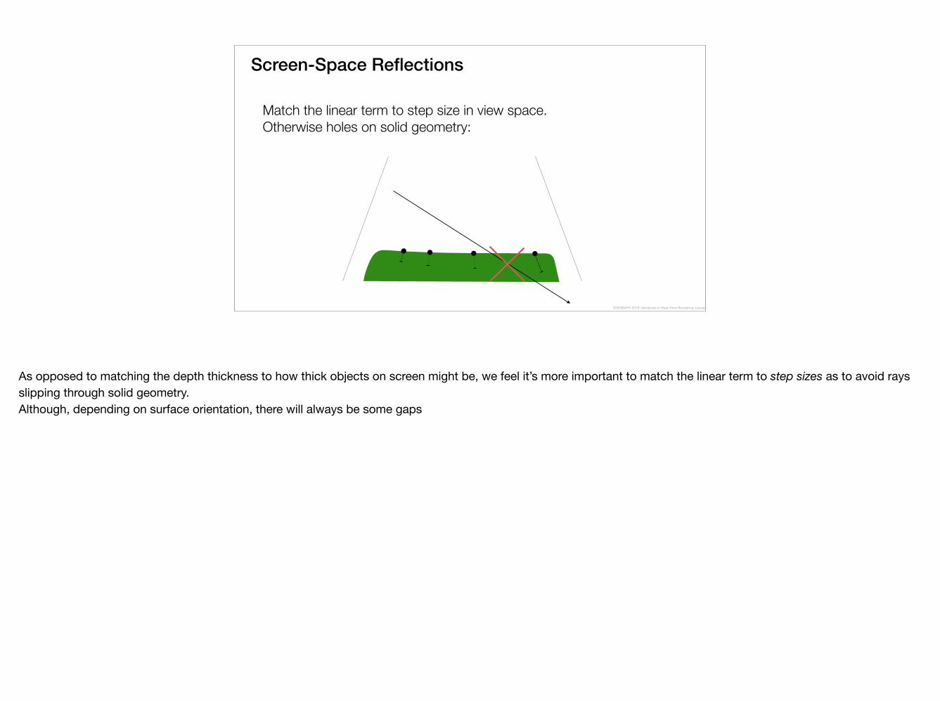
Match the linear term to step size in view space. Otherwise holes on solid geometry:
SIGGRAPH 2015: Advances in Real-Time Rendering course
As opposed to matching the depth thickness to how thick objects on screen might be, we feel it’s more important to match the linear term to step sizes as to avoid rays slipping through solid geometry.Although, depending on surface orientation, there will always be some gaps
Screen-Space Reflections
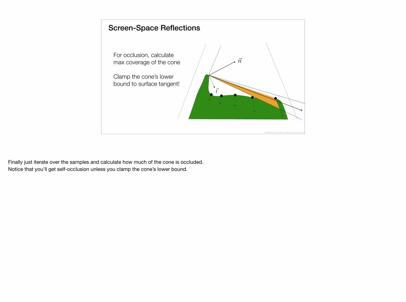
For occlusion, calculate max coverage of the coneClamp the cone’s lower bound to surface tangent!
~n
~t
SIGGRAPH 2015: Advances in Real-Time Rendering course
Finally just iterate over the samples and calculate how much of the cone is occluded.Notice that you’ll get self-occlusion unless you clamp the cone’s lower bound.
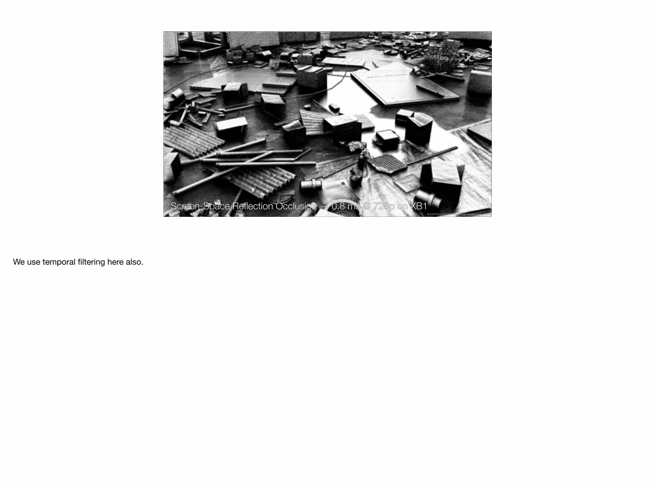
Screen-Space Reflection Occlusion — 0.8 ms @ 720p on XB1SIGGRAPH 2015: Advances in Real-Time Rendering course
We use temporal filtering here also.
Screen-Space Reflections
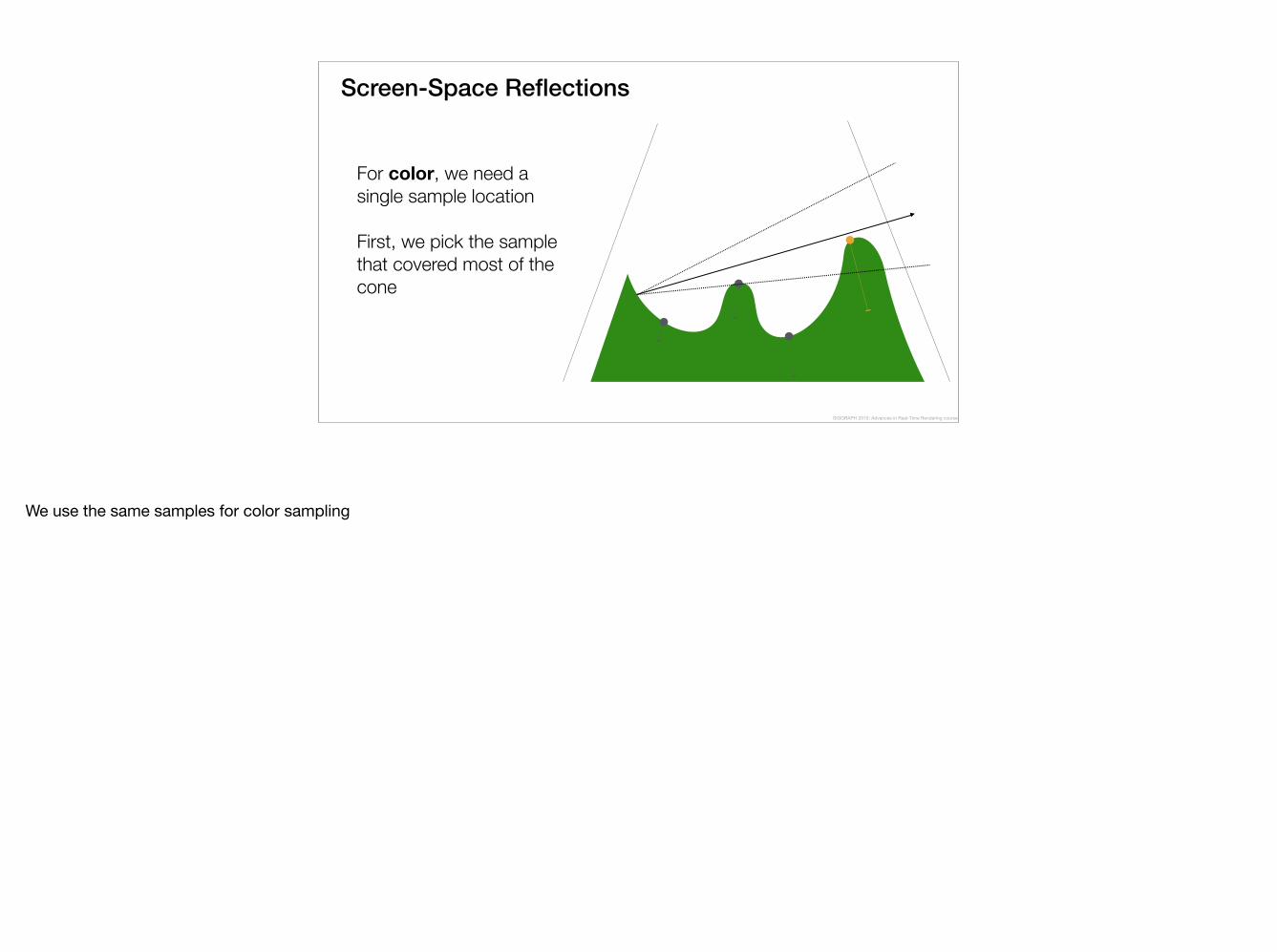
For color, we need a single sample locationFirst, we pick the sample that covered most of the cone
SIGGRAPH 2015: Advances in Real-Time Rendering course
We use the same samples for color sampling
Screen-Space Reflections
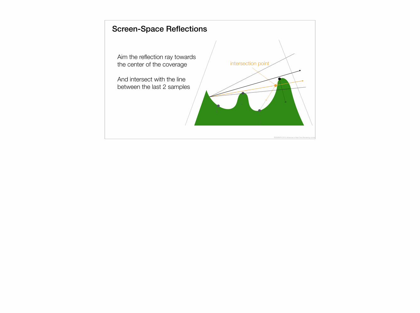
Aim the reflection ray towards the center of the coverageAnd intersect with the line between the last 2 samples
intersection point
SIGGRAPH 2015: Advances in Real-Time Rendering course

Screen-Space Reflections
Low sample density: interpolate towards camera direction (in blue)
intersection point
SIGGRAPH 2015: Advances in Real-Time Rendering course
We’re using 7 samples per pixel (low sample density), and the line between 2 consecutive samples will usually be too gently sloping. On average we can get a better match to geometry if we take the half vector between camera and 2 previous samples instead.
Screen-Space Reflections
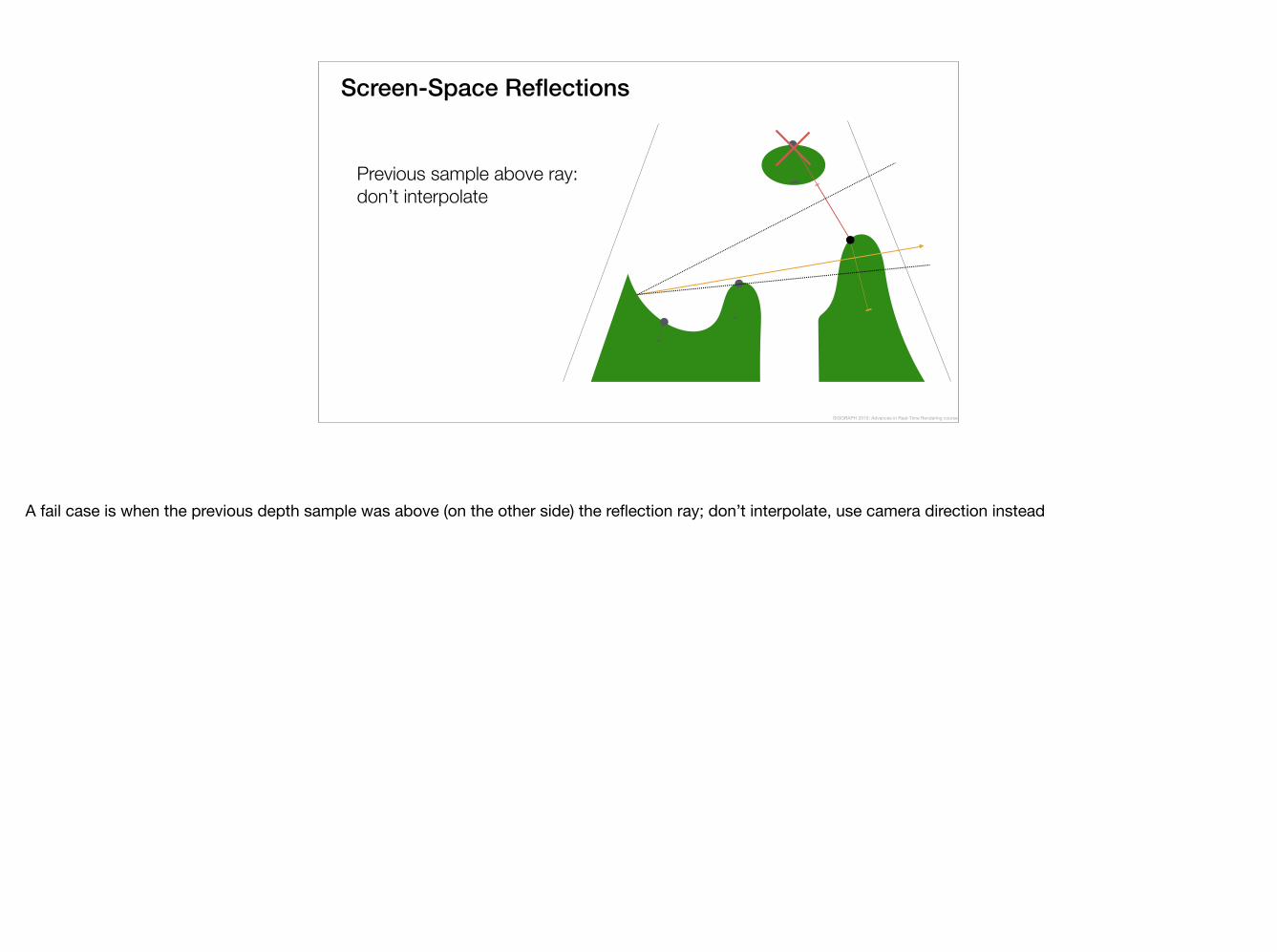
Previous sample above ray: don’t interpolate
SIGGRAPH 2015: Advances in Real-Time Rendering course
A fail case is when the previous depth sample was above (on the other side) the reflection ray; don’t interpolate, use camera direction instead

Screen-Space Reflections — 0.5 ms @ 720p on XB1
Final imageSIGGRAPH 2015: Advances in Real-Time Rendering course
Reproject the intersection point to previous frame and sample(MIP level = roughness * hit distance)Total render time for SSRO (0.8ms) and SSR (0.5ms) is 1.3ms
Screen-Space Ambient Occlusion 1.4ms @ 720p
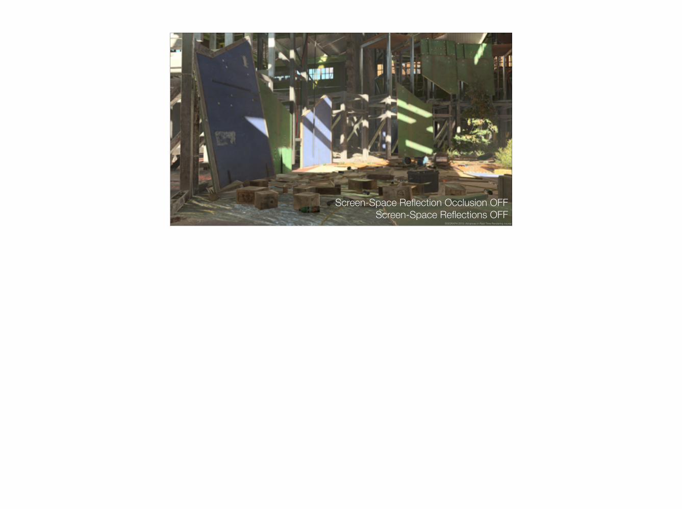
Screen-Space Reflection Occlusion OFFScreen-Space Reflections OFF
SIGGRAPH 2015: Advances in Real-Time Rendering course
Screen-Space Ambient Occlusion 1.4ms @ 720p
Screen-Space Reflection Occlusion ONScreen-Space Reflections OFF
SIGGRAPH 2015: Advances in Real-Time Rendering course

Screen-Space Ambient Occlusion 1.4ms @ 720p
Screen-Space Reflection Occlusion ONScreen-Space Reflections ON
SIGGRAPH 2015: Advances in Real-Time Rendering course
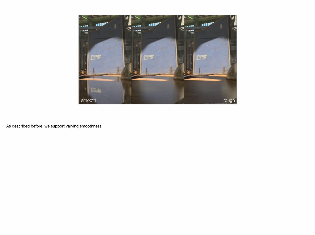
smooth roughSIGGRAPH 2015: Advances in Real-Time Rendering course
As described before, we support varying smoothness
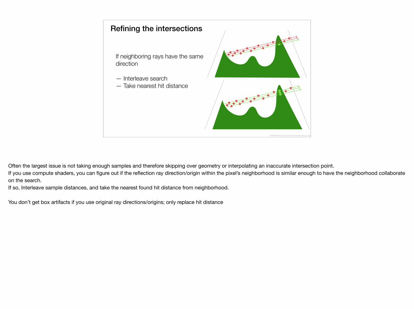
Refining the intersections
If neighboring rays have the same direction— Interleave search— Take nearest hit distance
SIGGRAPH 2015: Advances in Real-Time Rendering course
Often the largest issue is not taking enough samples and therefore skipping over geometry or interpolating an inaccurate intersection point.If you use compute shaders, you can figure out if the reflection ray direction/origin within the pixel’s neighborhood is similar enough to have the neighborhood collaborate on the search.If so, Interleave sample distances, and take the nearest found hit distance from neighborhood.
You don’t get box artifacts if you use original ray directions/origins; only replace hit distance
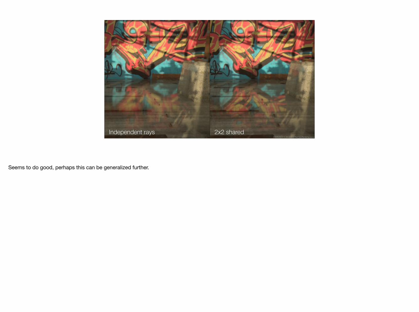
Independent rays 2x2 sharedSIGGRAPH 2015: Advances in Real-Time Rendering course
Seems to do good, perhaps this can be generalized further.
Acknowledgments Tatu AaltoJanne PulkkinenLaurent HarduinNatalya Tatarchuk Jaakko Lehtinen
Thank You!
SIGGRAPH 2015: Advances in Real-Time Rendering course
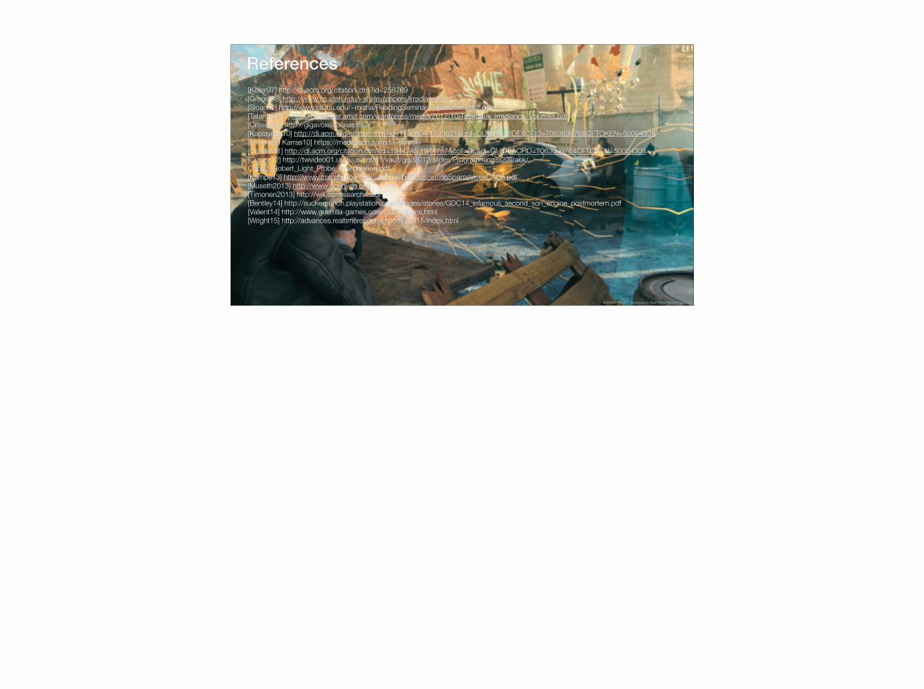
References[Keller97] http://dl.acm.org/citation.cfm?id=258769[Greger98] http://www.cs.utah.edu/~shirley/papers/irradiance.pdf [Sloan02] http://www.cs.jhu.edu/~misha/ReadingSeminar/Papers/Sloan02.pdf[Tatarchuk05] http://developer.amd.com/wordpress/media/2012/10/Tatarchuk_Irradiance_Volumes.pdf [Crassin09] http://gigavoxels.inrialpes.fr[Kaplaynan10] http://dl.acm.org/citation.cfm?id=1730804.1730821&coll=DL&dl=GUIDE&CFID=706369976&CFTOKEN=50004308[Laine and Karras10] https://mediatech.aalto.fi/~samuli/[Crassin11] http://dl.acm.org/citation.cfm?id=1944745.1944787&coll=DL&dl=GUIDE&CFID=706369976&CFTOKEN=50004308[Cupisz12] http://twvideo01.ubm-us.net/o1/vault/gdc2012/slides/Programming%20Track/Cupisz_Robert_Light_Probe_Interpolation.pdf[Kämpe13] http://www.cse.chalmers.se/~kampe/highResolutionSparseVoxelDAGs.pdf[Museth2013] http://www.openvdb.org[Timonen2013] http://wili.cc/research/lsao/[Bentley14] http://suckerpunch.playstation.com/images/stories/GDC14_infamous_second_son_engine_postmortem.pdf[Valient14] http://www.guerrilla-games.com/publications.html [Wright15] http://advances.realtimerendering.com/s2015/index.html
SIGGRAPH 2015: Advances in Real-Time Rendering course