1 CEEM, July 8-9, 2015

Which Specific Value of Demand-Response

Mechanisms

in Active Distribution Grids?

Cédric Clastres University of Grenoble – Alpes

CNRS, PACTE, EDDEN, CEEM

Patrice Geoffron University of Paris-Dauphine

LEDa-CEEM

2 CEEM, July 8-9, 2015

Preliminary results

Theoretical background and motivations

The model

Introduction

Outline

Conclusions and further developments

Appendices

3 CEEM, July 8-9, 2015

Introduction • Smart grids technologies will deeply modify distribution

and final consumers’ environment.

• Consumers’ adaptation to signals:

– Information.

– Prices.

• Potentially, a new “era” in electricity markets as demand

is usually seen as inelastic.

• In this context, Demand Response (DR) programs to be

developed, but:

– Which level of available DR?

– Which pricing schemes to value DR?

– Which allocation between “actors” of the power “value chain”?

4 CEEM, July 8-9, 2015

Preliminary results

Theoretical background and motivations

The model

Introduction

Outline

Conclusions and further developments

Appendices

5 CEEM, July 8-9, 2015

Dynamic pricing and elasticity

• Lijensen (2007):

– Consumers of electricity are captive in the short run.

• Haney & al. (2009), Faruqui & Sergici (2010):

– Demand could be elastic with SG and DR.

• Herter (2007):

– Consumers could be worse off with DR mechanisms (dynamic

pricing, critical peak pricing (CPP)).

– Consumers’ anticipate greater electricity bills increase with the use of

DR tools (also Park et al., 2014).

• Léautier (2014):

– Marginal value of Real Time Price (RTP) decreases with the number

of consumers “covered”.

6 CEEM, July 8-9, 2015

Examples of signals and load reductions

• Indirect feedback (education, information campaigns):

– Rather limited impact.

– 0 to 7% load reduction.

• Direct feedback (in home display, monitoring data from

smart meters):

– More significant.

– 2 to 15% load reduction.

• Dynamic pricing (with or without direct load control):

– Highest leverage.

– Up to 50% load reduction for some periods.

7 CEEM, July 8-9, 2015

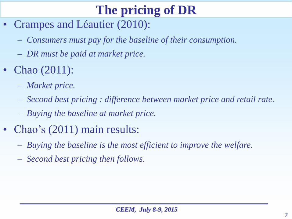
The pricing of DR • Crampes and Léautier (2010):

– Consumers must pay for the baseline of their consumption.

– DR must be paid at market price.

• Chao (2011):

– Market price.

– Second best pricing : difference between market price and retail rate.

– Buying the baseline at market price.

• Chao’s (2011) main results:

– Buying the baseline is the most efficient to improve the welfare.

– Second best pricing then follows.

8 CEEM, July 8-9, 2015

Motivations and main results • Objectives:

– Study DR programs under different pricing schemes in the French

context.

• Approach:

– Computing model with EPEX market data to simulate actors’ revenues.

– Relationships between actors are those of Chao (2011).

• Preliminary results:

– Demand response reductions are greater when DR is paid at market

price.

– To reduce peak demand, buying the baseline or second best pricing have

the same impact; only allocations of revenues differ.

– DR is profitable for welfare if total average costs are below 50€/MWh.

9 CEEM, July 8-9, 2015

Preliminary results

Theoretical background and motivations

The model

Introduction

Outline

Conclusions and further developments

Appendices

10 CEEM, July 8-9, 2015

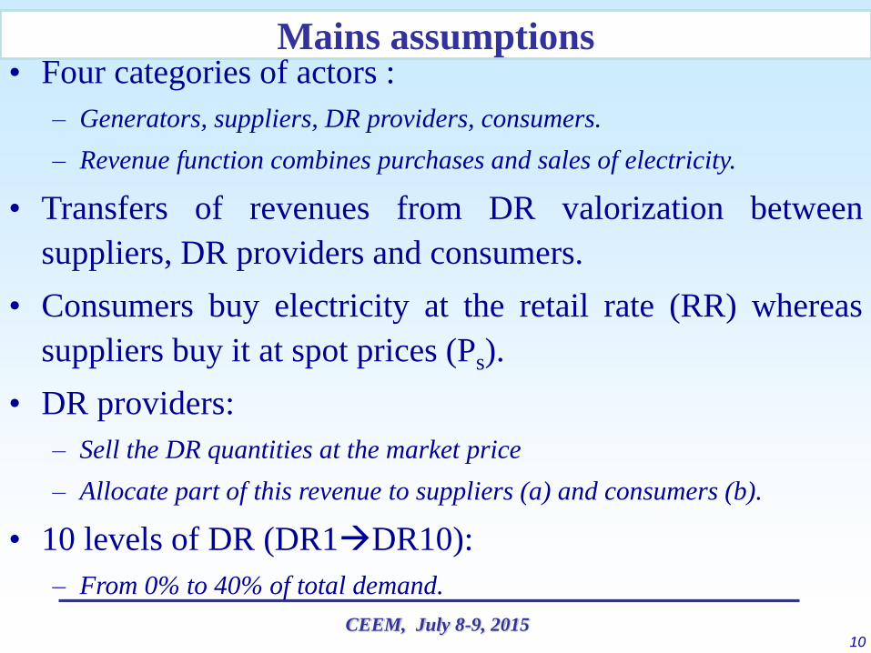
Mains assumptions • Four categories of actors :

– Generators, suppliers, DR providers, consumers.

– Revenue function combines purchases and sales of electricity.

• Transfers of revenues from DR valorization between

suppliers, DR providers and consumers.

• Consumers buy electricity at the retail rate (RR) whereas

suppliers buy it at spot prices (Ps).

• DR providers:

– Sell the DR quantities at the market price

– Allocate part of this revenue to suppliers (a) and consumers (b).

• 10 levels of DR (DR1DR10):

– From 0% to 40% of total demand.

11 CEEM, July 8-9, 2015

Three schemes of DR pricing (1/2) • Case 1:

– « Market price »

– DR at spot price (ps)

– pDR = ps (with ps >0)

• Case 2:

– « Buying the baseline »

– Consumers buy their consumption baseline at RR

– pDR = ps (with ps >RR)

• Case 3 :

– « Second best price »

– DR remuneration is the difference between spot price and retail rate

– pDR = ps – RR (with ps >RR)

12 CEEM, July 8-9, 2015

• In case 1, any load reduction is profitable for

consumers.

• In case 2 and 3, consumers reduce their consumption

if Ps> RR

• In case 2:

– They value their unit consumption at the RR because they buy

the baseline.

– If Ps< RR, they prefer to consume

• In case 3:

– Ps< RR leads to negative DR remuneration.

Three schemes of DR pricing (2/2)

13 CEEM, July 8-9, 2015

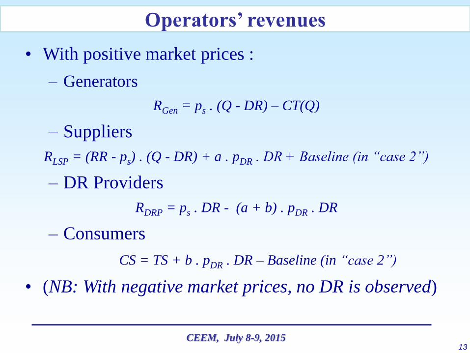
Operators’ revenues

• With positive market prices :

– Generators

RGen = ps . (Q - DR) – CT(Q)

– Suppliers

RLSP = (RR - ps) . (Q - DR) + a . pDR . DR + Baseline (in “case 2”)

– DR Providers

RDRP = ps . DR - (a + b) . pDR . DR

– Consumers

CS = TS + b . pDR . DR – Baseline (in “case 2”)

• (NB: With negative market prices, no DR is observed)

14 CEEM, July 8-9, 2015

Data

• We use data EPEX for 2014.

– Hourly prices and hourly quantities.

• Peak period is defined as hours 5PM to 8PM (“rush hours”

from EPEX)

• We use these data :

– to compute actor’s revenues in each pricing schemes;

– to determine the “implicit” break even point (revenues divided by

sales or consumed quantities).

15 CEEM, July 8-9, 2015

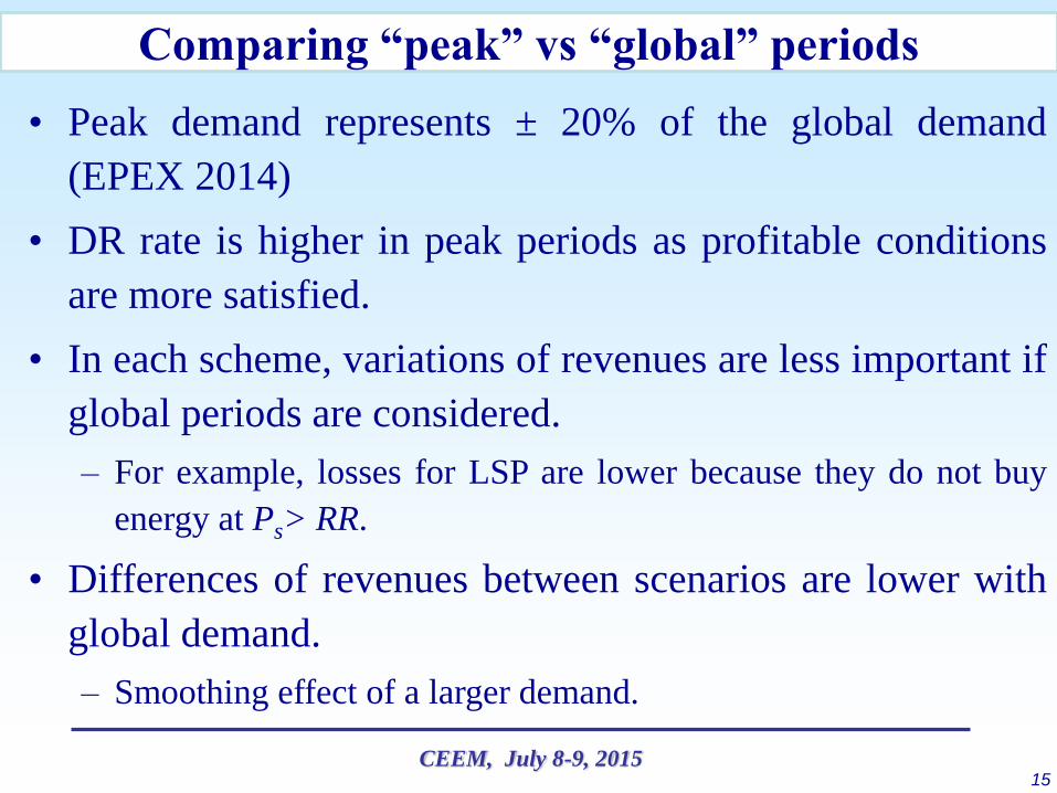
Comparing “peak” vs “global” periods

• Peak demand represents ± 20% of the global demand

(EPEX 2014)

• DR rate is higher in peak periods as profitable conditions

are more satisfied.

• In each scheme, variations of revenues are less important if

global periods are considered.

– For example, losses for LSP are lower because they do not buy

energy at Ps> RR.

• Differences of revenues between scenarios are lower with

global demand.

– Smoothing effect of a larger demand.

16 CEEM, July 8-9, 2015

Preliminary results

Theoretical background and motivations

The model

Introduction

Outline

Conclusions and further developments

Appendices

17 CEEM, July 8-9, 2015

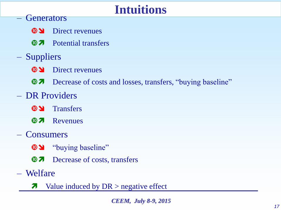
Intuitions – Generators

Direct revenues

Potential transfers

– Suppliers

Direct revenues

Decrease of costs and losses, transfers, “buying baseline”

– DR Providers

Transfers

Revenues

– Consumers

“buying baseline”

Decrease of costs, transfers

– Welfare

Value induced by DR > negative effect

18 CEEM, July 8-9, 2015

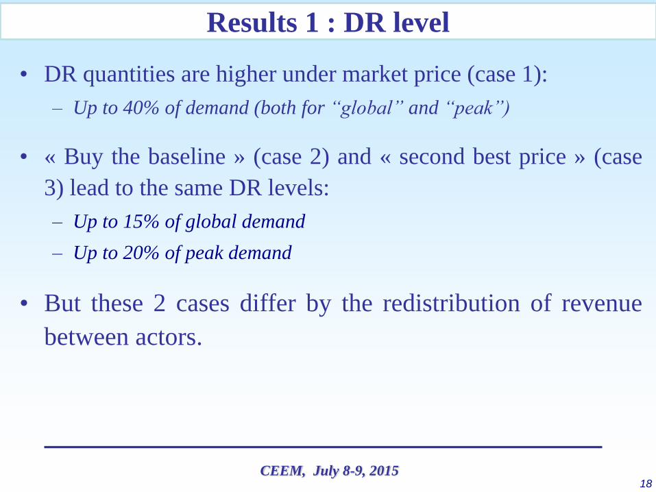
Results 1 : DR level

• DR quantities are higher under market price (case 1):

– Up to 40% of demand (both for “global” and “peak”)

• « Buy the baseline » (case 2) and « second best price » (case

3) lead to the same DR levels:

– Up to 15% of global demand

– Up to 20% of peak demand

• But these 2 cases differ by the redistribution of revenue

between actors.

19 CEEM, July 8-9, 2015

DR rate for each pricing scheme

0

5

10

15

20

25

30

35

40

45

DR1 DR2 DR3 DR4 DR5 DR6 DR7 DR8 DR9 DR10

Market price

Second bestprice/BuyBaseline(global demand)

Second bestprice/BuyBaseline(peak demand)

(%)

20 CEEM, July 8-9, 2015

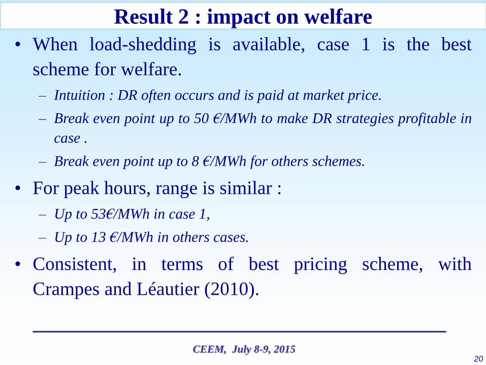
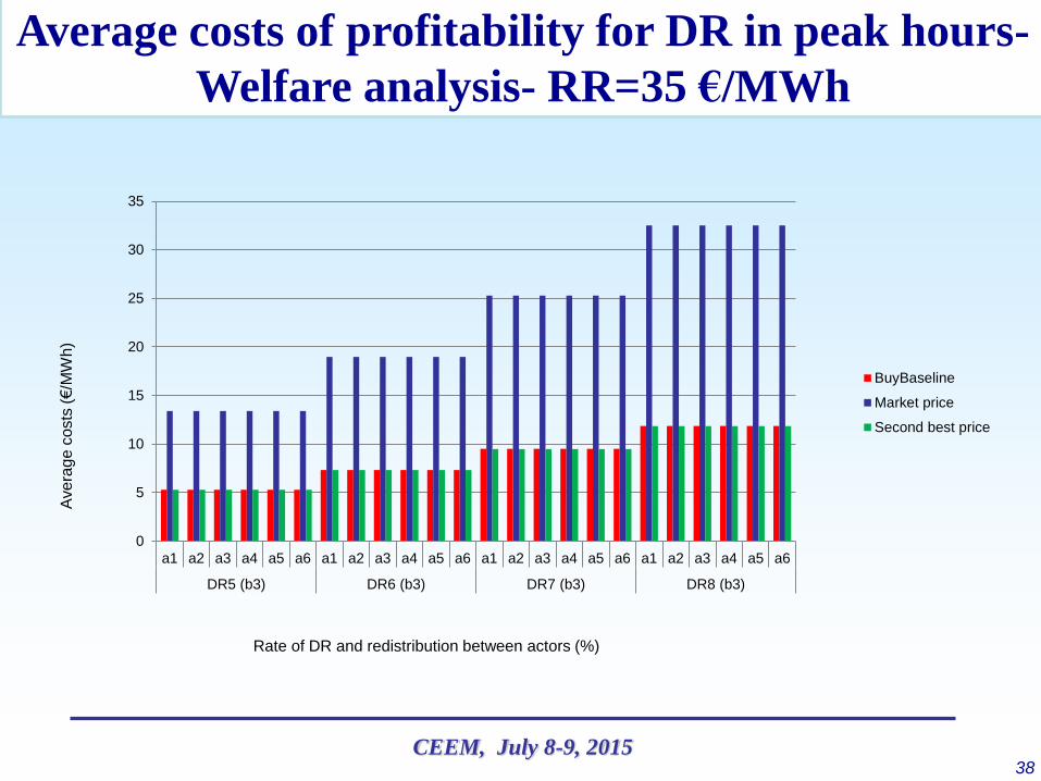
Result 2 : impact on welfare

• When load-shedding is available, case 1 is the best

scheme for welfare.

– Intuition : DR often occurs and is paid at market price.

– Break even point up to 50 €/MWh to make DR strategies profitable in

case .

– Break even point up to 8 €/MWh for others schemes.

• For peak hours, range is similar :

– Up to 53€/MWh in case 1,

– Up to 13 €/MWh in others cases.

• Consistent, in terms of best pricing scheme, with

Crampes and Léautier (2010).

21 CEEM, July 8-9, 2015

Break even for DR in peak hours: Welfare analysis

0

5

10

15

20

25

30

35

40

a1 a2 a3 a4 a5 a6 a1 a2 a3 a4 a5 a6 a1 a2 a3 a4 a5 a6 a1 a2 a3 a4 a5 a6

DR5 (b3) DR6 (b3) DR7 (b3) DR8 (b3)

BuyBaseline

Market price

Second best price

Rate of DR and redistribution between actors (%)

Ave

rag

e c

osts

(€/M

Wh

)

22 CEEM, July 8-9, 2015

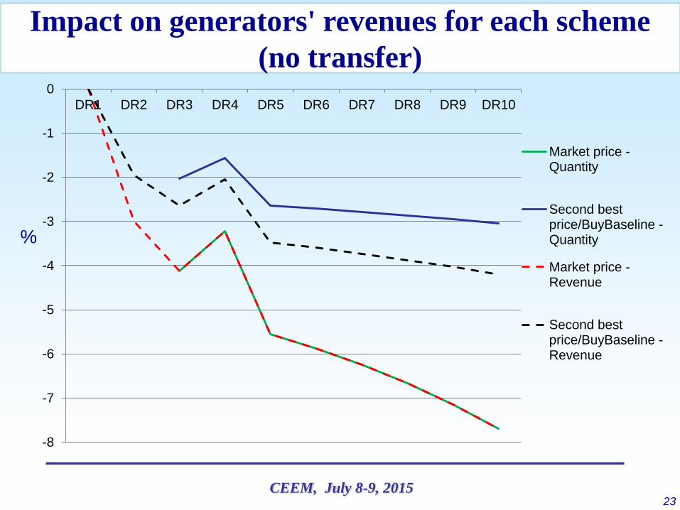
Results 3 : focus on generators

• DR imply transfers towards generators to compensate direct

revenue losses (quantity effect).

• The break even is a decreasing function of the DR rate for

case 2 and 3 :

– 32 to 35€/MWh for global demand.

– 37 to 40 €/MWh for peak demand.

• For case 1, break even is constant :

– 35€/MWh for global demand.

– 40€/MWh for peak demand.

23 CEEM, July 8-9, 2015

Impact on generators' revenues for each scheme

(no transfer)

-8

-7

-6

-5

-4

-3

-2

-1

0

DR1 DR2 DR3 DR4 DR5 DR6 DR7 DR8 DR9 DR10

Market price -Quantity

Second bestprice/BuyBaseline -Quantity

Market price -Revenue

Second bestprice/BuyBaseline -Revenue

%

24 CEEM, July 8-9, 2015

Results 4 : case 2 vs case 3 (suppliers)

• For suppliers :

– Case 2 leads to greater revenues:

• Up to 30% for global hours

• Higher than 100% for only peak hours

– Break even:

• Up to 5€/MWh (case 3) or up to 8€/MWh (case 2) for global hours,

• Up to 4€/MWh (case 3) or up to 12€/MWh (case 2) for peak hours,

– Intuition :

• Buying the baseline means additional revenues for suppliers.

• Moreover, DR is paid at market price in case 2, whereas it is paid

at second best price in case 3.

• Thus redistribution of DR revenues is higher in case 2.

25 CEEM, July 8-9, 2015

Variations of suppliers' revenues between pricing

schemes (global demand): DR2 to DR4

-20

-10

0

10

20

30

40

50

60

a1 a2 a3 a4 a5 a6 a1 a2 a3 a4 a5 a6 a1 a2 a3 a4 a5 a6

DR 2 DR 3 DR 4

Second bestprice/Marketprice

BuyBaseline/Market price

BuyBaseline/Second bestprice%

26 CEEM, July 8-9, 2015

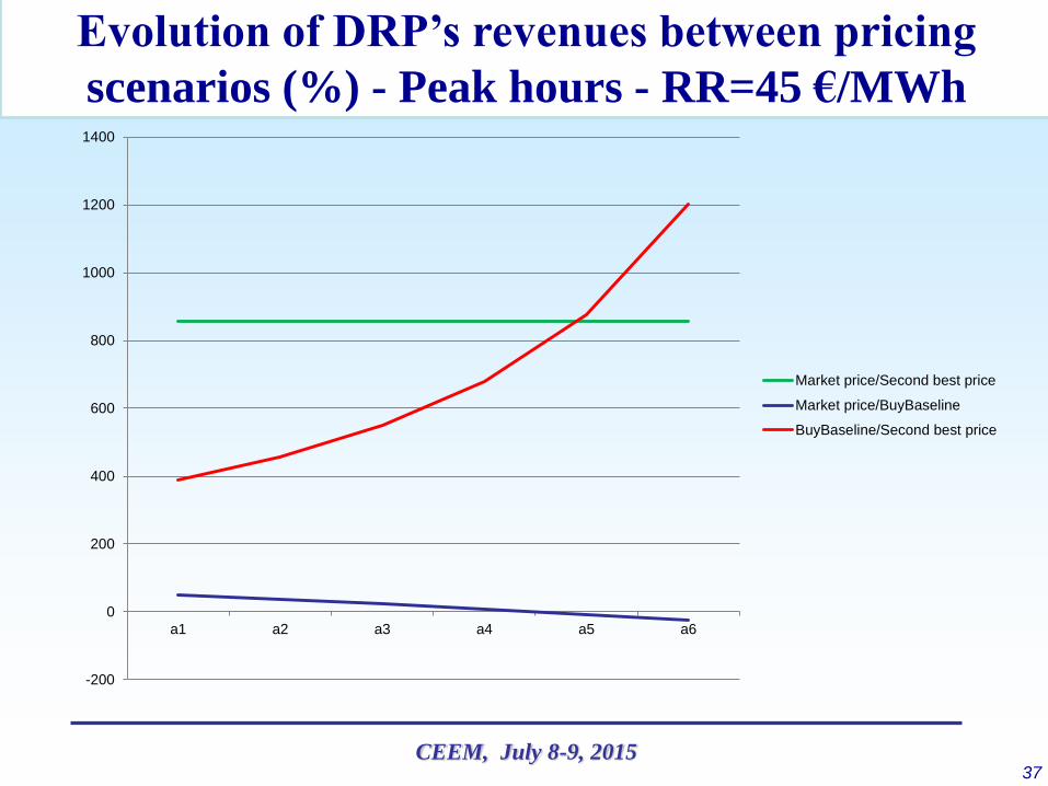
Results 5 : case 2 vs case 3 (DRP)

• For DRP :

– Case 2 leads to higher revenues

• Higher than 400% for global hours.

• Higher that 100 % for only peak hours.

– Break even:

• Up to 10€/MWh (case 3) or up to 50€/MWh (case 2) for global hours.

• Up to 12€/MWh (case 3) or up to 52€/MWh (case 2) for peak hours.

– Intuition :

• DRP do not have to distribute DR revenue to suppliers because of the

purchase of the baseline by consumers.

• Thus, its revenues increase.

27 CEEM, July 8-9, 2015

DRP’s revenues between pricing schemes:

Peak hours

-200

0

200

400

600

800

1000

1200

a1 a2 a3 a4 a5 a6

Market price/Secondbest price

Marketprice/BuyBaseline

BuyBaseline/Secondbest price

%

28 CEEM, July 8-9, 2015

Results 6 : case 2 vs case 3 (consumers) • For consumers:

– The contrary to the two others actors.

– Case 3 leads to higher revenues

• Up to 8% for global hours

• Up to 66% for only peak hours

– Intuition : consumers do not buy the baseline (lower costs).

– To make DR strategies profitable, surplus by unit consumed

quantity must be higher than :

• Up to 39€/MWh (case 3) or up to 40€/MWh (case 2) for global hours,

• Up to 39€/MWh (case 3) or up to 50€/MWh (case 2) for peak hours,

29 CEEM, July 8-9, 2015

Consumer's revenue between pricing schemes:

global demand

-35

-30

-25

-20

-15

-10

-5

0

b1 b2 b3 b4 b5 b6 b1 b2 b3 b4 b5 b6 b1 b2 b3 b4 b5 b6

DR 2 DR 3 DR 4

Second bestprice/Market Price

BuyBaseline/MarketPrice

BuyBaseline/Secondbest price

%

30 CEEM, July 8-9, 2015

Preliminary results

Theoretical background and motivations

The model

Introduction

Outline

Conclusions and further developments

Appendices

31 CEEM, July 8-9, 2015

Conclusion • Very preliminary results to be “refined”

• DR pricing schemes impact the level of available DR.

• Promoting DR programs with appropriate pricing

schemes could improve the welfare.

• Allocation of DR revenues: - important to combine opposed interests

- and consumers’ fears of increasing bills.

• The break even point is “high” in some cases…

32 CEEM, July 8-9, 2015

Further developments

• Introduction of generation costs and consumers’ surplus with

supply and demand curves from EPEX.

• Simulation with an impact of DR on the fixing procedure

(with the use of supply and demand curves).

• Demand segmentation (all consumers do not have the same

level of available DR quantities).

• Splitting hours of the days in different periods to implement

load-shifting and the rebound effects.

• Introduction of the valorization of DR on balancing market.

• The TSO/DSO are not included (potential impact on CAPEX

and OPEX and, then, on DR benefits)

33 CEEM, July 8-9, 2015

Preliminary results

Theoretical background and motivations

The model

Introduction

Outline

Conclusions and further developments

Appendices

34 CEEM, July 8-9, 2015

≠ of suppliers' revenues between pricing schemes

(global demand) - DR2 to DR4 - RR=35€/MWh

-20

-10

0

10

20

30

40

50

60

a1 a2 a3 a4 a5 a6 a1 a2 a3 a4 a5 a6 a1 a2 a3 a4 a5 a6

DR 2 DR 3 DR 4

Second best price/Market price

BuyBaseline/Market price

BuyBaseline/Second best price

35 CEEM, July 8-9, 2015

-10

-5

0

5

10

15

20

25

30

a1 a2 a3 a4 a5 a6 a1 a2 a3 a4 a5 a6 a1 a2 a3 a4 a5 a6

DR 2 DR 3 DR 4

Second best price/Market price

BuyBaseline/Market price

BuyBaseline/Second best price

≠ of suppliers' revenues between pricing scenario

(global demand) - DR2 to DR4 - RR=45€

36 CEEM, July 8-9, 2015

-100

0

100

200

300

400

500

600

700

800

900

a1 a2 a3 a4 a5 a6

Market price/Second best price

Market price/BuyBaseline

BuyBaseline/Second best price

Evolution of DRP’s revenues between pricing

scenarios (%) - Peak hours - RR=35 €/MWh

37 CEEM, July 8-9, 2015

-200

0

200

400

600

800

1000

1200

1400

a1 a2 a3 a4 a5 a6

Market price/Second best price

Market price/BuyBaseline

BuyBaseline/Second best price

Evolution of DRP’s revenues between pricing

scenarios (%) - Peak hours - RR=45 €/MWh

38 CEEM, July 8-9, 2015

0

5

10

15

20

25

30

35

a1 a2 a3 a4 a5 a6 a1 a2 a3 a4 a5 a6 a1 a2 a3 a4 a5 a6 a1 a2 a3 a4 a5 a6

DR5 (b3) DR6 (b3) DR7 (b3) DR8 (b3)

BuyBaseline

Market price

Second best price

Rate of DR and redistribution between actors (%)

Avera

ge c

osts

(€/M

Wh)

Average costs of profitability for DR in peak hours-

Welfare analysis- RR=35 €/MWh

39 CEEM, July 8-9, 2015

References

• Chao H. P., (2010). "Price responsive demand management for smart grid world".

Electricity Journal, vol. 23, n° 1, pp. 7-20.

• Chao H. P., (2011). "Demand Response in wholesale electricity markets: the choice of

customer baseline". Journal of Regulatory Economics, vol. 39, n° 1, p. 68- 88.

• Crampes C., Léautier T.O., (2010). Dispatching et effacement de demande. Toulouse :

Institut d’Economie Industrielle.

• Faruqui, A., Sergici, S., (2010). Household response to dynamic pricing of electricity: a

survey of 15 experiments. J. Regul. Econ. 38 (2)

• Herter, K. (2007).Residential implementation of critical-peak pricing of electricity,

Energy Policy, 35:4, April, 2121-2130.

• Haney, A.B., Jamasb, T., Pollitt, M.G., (2009). Smart Metering and Electricity Demand:

Technology, Economics and International Experience. Electricity Policy Research

Group, Cambridge, Working Paper EPRG0903.

• Lijesen Mark G., (2007) The real-time price elasticity of electricity, Energy Economics,

Volume 29, Issue 2..

• Park, C-K., Kim H-J., Kim Y-S. (2014), “A study factor enhancing smart grid consumer

engagement”, Energy Policy, 72.

40 CEEM, July 8-9, 2015

Thanks for your attention