Which Ladder to Climb?Decomposing Life-Cycle Wage Dynamics∗

Christian Bayer† Moritz Kuhn‡

October 9, 2020

Abstract

Wages grow and become more unequal as workers age. Decomposing these life-cycle wage dynamics into factors like education, labor market experience, employerdifferences, and occupations, we find job levels to be the most important source.Climbing the career ladder to higher job levels accounts for half of average wagegrowth and virtually all of rising life-cycle dispersion. Job levels describe the au-tonomy, responsibility, and complexity in executing a job’s tasks and duties andwe discuss their economic content, measurement, and how they differ from occu-pations and education. Exploring career ladder dynamics, we find that most stepson the career ladder happen with the same employer but that employer changesaccelerate climbing the career ladder. We offer a career ladder perspective on styl-ized wage facts by revisiting the gender wage gap, returns to education, employerwage differences, and returns to seniority.

Keywords: life cycle wage growth, wage inequality, career ladderJEL Codes: D33, E24, J31.

∗We thank Jim Albrecht, Thomas Dohmen, Jan Eeckhout, Simon Jäger, Fatih Karahan, Greg Kaplan,Francis Kramarz, Iourii Manovskii, Simon Mongey, Elena Pastorino, Esteban Rossi-Hansberg, ToddSchoellman, Ludo Visschers, Michael Waldman, and conference and seminar participants at variousplaces. The authors gratefully acknowledge support through the project ADEMU, “A Dynamic Economicand Monetary Union,” funded by the European Union’s Horizon 2020 Program under grant agreementNo. 649396 and the Deutsche Forschungsgemeinschaft (DFG, German Research Foundation) underGermany´s Excellence Strategy – EXC 2126/1– 390838866. Bayer would like to thank the EUI forhosting him while conducting part of the research that led to this paper. Kuhn would like to thank theFederal Reserve Bank of Minneapolis for hosting him while conducting part of the research that led tothis paper. A previous version has been circulated as “Which Ladder to Climb? Wages of Workers byJob, Plant, and Education.”

†Universität Bonn, CEPR, and IZA, Adenauerallee 24-42, 53113 Bonn, Germany, email:christian.bayer@uni-bonn.de

‡Universität Bonn, ECONtribute, CEPR, and IZA, Adenauerallee 24-42, 53113 Bonn, Germany,email: mokuhn@uni-bonn.de

1 Introduction

Why do wages grow and become more unequal as workers age? We revisit this questionon the sources of life-cycle wage dynamics using new data and provide new answers. Westart from economic theory and account for key sources of life-cycle wage dynamics like aworker’s education, labor market experience, employer differences, and occupations. Still,we find another largely unexplored job characteristic, the job level, to be the single mostimportant driver of life-cycle wage dynamics. While career ladder dynamics have beenstudied in case studies for single employers before (Baker et al.Baker et al., 19941994), their importancefor life-cycle wage dynamics at the level of the macroeconomy have not yet been explored.The aim of the paper is to fill this void.What is the job level of a job? Occupations describe which tasks a worker has to execute inher job and have been widely studied in economic research (e.g. Kambourov and ManovskiiKambourov and Manovskii,2009a2009a; Autor et al.Autor et al., 20032003). Job levels provide an additional distinction of jobs regardingautonomy, responsibility, and complexity when executing a job’s tasks. For the simplestexample of such differences consider two bakers. One of them is following recipes andrules for mixing and baking dough. The other baker also mixes ingredients and bakesdoughs but develops new recipes. Both perform the occupational tasks of bakers, yet,their job levels will differ.11 Conceptually, we think of occupations as an extensive marginof task execution (which tasks are done) and of job levels as an intensive margin of taskexecution (how are tasks done). Importantly, job levels provide a consistent distinctionof this intensive margin variation for all jobs in the labor market.In the main part of our analysis, we explore data from three waves of the German Struc-ture of Earnings Survey (SES) from 2006 to 2014 that include information on job levels.These data provide a powerful opportunity to decompose life-cycle wage dynamics sinceobservable characteristics account for over 80% of wage variation in these data. Wedocument that climbing the career ladder, transiting across job levels as workers age,accounts for 50% of wage growth for males and females and almost all of the increasein wage dispersion over the life cycle. Based on these findings, we then provide newstructural interpretations of widely studied wage phenomena such as the gender wagegap, returns to education, employer wage differences, and returns to seniority.To explore the economic content of job levels, we use data on job requirements from theBIBB/BAuA Employment Survey. In these data, we construct from reported job require-ments the job-leveling factors that are the building blocks to constructing job levels. Bymeasuring the intensive margin of task execution directly, we find that the job-levelingfactors account for 44% of wage dispersion in the BIBB/BAuA data. To demonstrate

1For a complete list of tasks for bakers, see https://www.onetonline.org/link/summary/51-3011.00https://www.onetonline.org/link/summary/51-3011.00.

1

how job levels differ from occupations, we document in the SES data that the typicaloccupation has substantial employment shares on three job levels and that job levelsaccount for a substantial part of wage dispersion within and across occupations. We alsodiscuss the relationship to the task-based approach (Autor et al.Autor et al., 20032003) and find thattask-related wage differences are largely absorbed by average job-level differences so thattask-based (occupational) wage components account for only a little of wage dispersiononce job levels are controlled for. Information on job levels as in the SES data is onlyavailable in a few other datasets so that we conjecture that this absence is one of themain reasons why their explanatory power for wages remained largely unexplored. Forthe United States, the National Compensation Survey (NCS) conducted by the Bureauof Labor Statistics (BLS) is a dataset that also provides data on job levels and similarlystriking results on the explanatory power of job levels for wages apply (PiercePierce, 19991999). Inthe NCS data, job-leveling factors account for 75% of the cross-sectional wage dispersionand about half of the within-occupation wage dispersion; furthermore, job levels accountfor virtually all of the observed between-occupation wage differences. When we repeatthese decompositions in the SES data, we find very similar results. Based on this addi-tional evidence, we conclude that the importance of job levels for macroeconomic wagedifferences is neither a particularity of the administrative data nor the German labormarket.To put our results into perspective, we note that encoded job levels comprise more thanour simplistic baker example above suggests. Job levels combine several aspects aboutthe execution of tasks.22 One of those aspects is that some jobs feature a (particularly)complex set of tasks which becomes apparent in some minimum skill requirements. Yet,A minimum skill requirement still allows for situations where workers with a college edu-cation are cab drivers as long as they have the minimum requirement of a driver’s license.This fact relates job levels to human capital as it provides a notion of human capitalutilization on the job, e.g., a cab driver with a college education would not use all of herhuman capital.33 It also highlights the underlying idea of wage determination, namely,that workers get paid for the tasks they deliver rather than for their stock of human cap-ital. This idea is not new and also not original to job levels but, as Acemoglu and AutorAcemoglu and Autor(20122012) note, a key innovation of the task-based approach proposed in Autor et al.Autor et al. (20032003).Acemoglu and AutorAcemoglu and Autor (20122012) emphasize that the focus on task execution for wage determi-nation is the key distinction between a traditional human capital view and the task-basedapproach. The second key aspect encoded in the job level is autonomy in the execution

2See US Bureau of Labor StatisticsUS Bureau of Labor Statistics (20132013) for a detailed description of job leveling in the US NCSdata.

3RosenRosen (19831983) explores the consequences of an on-the-job human capital utilization decision for humancapital investment.

2

of tasks. Our initial baker example provides an example of this aspect as the two workersdiffer in how closely they have to follow rules and procedures in the execution of theirtasks. Finally, the responsibility aspect of the job level captures the scale of operationsaffected by the jobholder’s task execution. For example, if a supervisor directs a team ofa few workers her responsibility is lower compared to a manager whose orders bind theactivities of workers in the entire firm even if the manager herself supervises only few orno workers directly. Although job levels are independent of specific occupational tasks,i.e., baking bread or making sausages, it is also clear that, for example, management occu-pations have, by construction, higher job levels. Hence, we should expect that job levelscorrelate with occupations and with other occupation-derived concepts like the task-basedapproach (Autor et al.Autor et al., 20032003) or within-firm hierarchies (Garicano and Rossi-HansbergGaricano and Rossi-Hansberg,20062006).The analyzed SES data come as repeated cross sections and we apply synthetic panelmethods (DeatonDeaton, 19851985; VerbeekVerbeek, 20082008) as a standard tool from the macroeconomictoolkit to decompose life-cycle wage dynamics in these data. We construct the panel dataat the cohort level from the repeated cross sections and estimate the coefficients of inter-est based on cohort-level wage regression. We use the estimated coefficients to constructworker-level wage components arising from observable individual and job characteristicsplus an employer component. Using this decomposition, we document how importanteach component is for wage growth and wage dispersion over the life cycle. We provideseparate decompositions for males and females as interesting differences arise. We fur-ther decompose the contribution of job characteristics into an intensive margin (job level)component and an extensive margin (occupation) component and find that the formeraccounts for virtually the entire job component.Our analysis has to address two key identification challenges that are motivated by theo-retical models of career progression. The first challenge results from the seminal work byWaldmanWaldman (19841984) and refined by Gibbons and WaldmanGibbons and Waldman (20062006). In this model framework,employers learn about workers’ abilities and promote good (highly productive) workersto jobs with potentially higher skill requirements and higher skill complementarity. Highwages are then the means to prevent other employers from poaching highly productiveworkers. A worker’s productivity is the key determinant of wages and high-paying jobsare only a signal that the jobholder is a highly productive worker. We address the arisingchallenge that unobserved individual heterogeneity is accounting for the wage differencesacross job levels in three ways. First, we aggregate the data to the cohort level so that weexploit only the differential distribution of cohorts across job levels for identification. Sec-ond, these cohorts might still differ in their (average) individual fixed effects and careerprogression. Controlling for fixed effects in our panel regression removes this challenge

3

for identification. Third, we apply an instrumental variable approach based on shifts inindustry composition over time. We find very similar results for the importance of joblevels for wage dynamics based on this approach.The second challenge for identification arises from the mechanism highlighted in the sem-inal paper by Lazear and RosenLazear and Rosen (19811981). Lazear and RosenLazear and Rosen provide an alternative view oncareer progression that interprets promotions as the outcome of a tournament. Consid-ering jobs and the associated wages as prizes implies that changes in a job’s tasks are notsystematically related to wages, as wages only represent a prize for previous performancebut not a remuneration for task execution on the current job. We exploit the BIBB/BAuAdata with detailed information on task execution at the worker level to provide evidencethat job levels describing these differences in task execution have economic content andare systematically related to wages. Put differently, we find a fundamental role for a job’stask execution in determining wages. Such an important role for job content aligns closelywith the key ideas of the task-based approach (Autor et al.Autor et al., 20032003; Acemoglu and AutorAcemoglu and Autor,20122012) but also with the large literature on the effect of technological change on the wagestructure (e.g., Katz and AutorKatz and Autor, 19991999; Krusell et al.Krusell et al., 20002000).What we do not answer in this paper is the question of why workers end up in the jobsthey have and why some climb the career ladder while others do not. In this sense, weexplore the consequences rather than the causes of career progression. We still explorecareer dynamics over the life cycle by complementing our cross-sectional analysis withpanel evidence from the German Socio-economic Panel data (SOEP) where we observea proxy for job levels. We document life-cycle profiles of career ladder promotion anddemotion rates and explore how labor market mobility across employers and throughnonemployment is related to steps up and down the career ladder. We find that employermobility is associated with career progression but that most steps on the career ladderhappen while staying with the same employer. We also explore luck as one potentialdriver of career dynamics and find that the presence of an older peer (silverback) as acompetitor for promotion in a plant significantly hinders career progression.We build on our empirical finding on the importance of the career ladder for life-cyclewage dynamics to provide a new perspective on stylized wage facts. Taking a career-ladder perspective, we revisit the gender pay gap, the returns to education, employer paydifferences, and the returns to seniority (Buhai et al.Buhai et al., 20142014). The high explanatory powerof observables allows us, for example, to trace back the estimated gender wage gap todifferences in life-cycle career progression. We demonstrate that the widening gender wagegap by age results from increasing job-level differences across gender that turn the genderwage gap into a gender promotion gap. Similarly, we revisit the returns to education anddemonstrate that we can relate differences in wage growth across education groups to

4

differences in promotion patterns. Using our empirical results, we directly relate differenteducation levels to differences in career ladder dynamics and account for the resultingreturns to education. As a third wage fact, we revisit employer pay differences that havebeen widely studied following the influential work by Abowd et al.Abowd et al. (19991999). The differentestimation approaches make our estimates for employer wage components not directlycomparable, but we provide corroborating evidence for the ideas in Card et al.Card et al. (20132013)and Song et al.Song et al. (20152015) that the composition of jobs constitutes one important reason foraverage employer wage differences in the data. Specifically, we document large changes inour decomposition of life-cycle wage dynamics if we do not account for job compositionacross employers. We find that employer differences become much more important forlife-cycle wage growth and rising wage dispersion once job controls are excluded from thedecomposition. Finally, we also explore returns to seniority (Buhai et al.Buhai et al., 20142014) throughthe lens of career ladder dynamics. We find that three-quarters of an estimated senioritywage premium is accounted for by being higher up on the career ladder rather than adirect effect of seniority on wages.The remainder of the paper is organized as follows: We relate our work to the existingliterature in Section 22. Section 33 introduces the data and provides further details on joblevels. Section 44 reports our main decomposition results for life-cycle wage dynamics. InSection 55, we provide a new perspective on wage dynamics by discussing the implicationsfrom our empirical analysis. We conclude with Section 66. An appendix follows.

2 Related literature

By exploring the sources of life-cycle wage growth and inequality, we relate our worktothe long-standing economic research agenda on determinants of wage differences goingback at least to the seminal work of MincerMincer (19741974). His work has developed into alarge literature that documented a variety of life-cycle wage growth and inequality pat-terns (for example, Deaton and PaxsonDeaton and Paxson, 19941994; Storesletten et al.Storesletten et al., 20042004; Heathcote et al.Heathcote et al.,20052005; Huggett et al.Huggett et al., 20062006). A common practice today is to interpret the residuals fromMincerian wage regressions as wage risk and a large body of literature is devoted toestimating stochastic processes for these residuals (Lillard and WillisLillard and Willis, 19781978; MaCurdyMaCurdy,19821982; Carroll and SamwickCarroll and Samwick, 19971997; Meghir and PistaferriMeghir and Pistaferri, 20042004; GuvenenGuvenen, 20092009). Recently,Huggett et al.Huggett et al. (20112011), Guvenen and SmithGuvenen and Smith (20142014) and Bagger et al.Bagger et al. (20142014) took morestructural approaches to explore the drivers of life-cycle inequality. We add to this liter-ature by relating diverging wages to observable steps on the career ladder and differencesbetween employers. Kambourov and ManovskiiKambourov and Manovskii (20082008, 2009a2009a,bb) document an important

5

role of occupations as a determinant of wage differences in the cross section and overtime. Low et al.Low et al. (20102010), Hornstein et al.Hornstein et al. (20112011), or Jung and KuhnJung and Kuhn (20162016) explore em-ployer differences as a source of earnings inequality in search models.Our findings are also closely related to the personnel economics literature that studies in-ternal labor markets and career dynamics following the seminal work of Doeringer and PioreDoeringer and Piore(19851985). The existing research in this strand of literature relies on case studies of singlefirms and sometimes even subgroups of workers at those firms as in Baker et al.Baker et al. (19941994).Baker et al.Baker et al. (19941994) and Dohmen et al.Dohmen et al. (20042004) find that, absent promotions across joblevels, there is virtually no individual wage growth. Gibbs et al.Gibbs et al. (20032003) and FoxFox (20092009)document for Sweden that promotions are a key source of life-cycle earnings growth andBronson and ThoursieBronson and Thoursie (20182018) document also in Swedish panel data gender differences incareer progression.44 This strand of the literature unanimously echoes the key idea formu-lated in Doeringer and PioreDoeringer and Piore (19851985, p. 77) that “[i]n many jobs in the economy, wagesare not attached to workers, but to jobs.”Regarding theoretical career-ladder models, WaldmanWaldman (20122012) provide an excellent overview.The seminal papers are Lazear and RosenLazear and Rosen (19811981), who explain promotion dynamics as aresult of tournaments, and WaldmanWaldman (19841984), who emphasizes the signaling role of promo-tions in an environment with asymmetric information about workers’ ability. Gibbons et al.Gibbons et al.(20062006) and Gibbons and WaldmanGibbons and Waldman (20062006) extend this theory by allowing for a skill job-level complementarity. As summarized in Rubinstein and WeissRubinstein and Weiss (20062006), the underlyingassumption of these theories is that wage differences stem exclusively from worker skillspotentially magnified by job assignments rendering skills differently productive.55

An alternative macroeconomic approach puts the organizational structure of firms at thecenter of the analysis. Caicedo et al.Caicedo et al. (20182018) study secular trends in the wage structureand propose a theory of vertical job differentiation as a result of specialization in theproduction process. Caliendo et al.Caliendo et al. (20152015) provide empirical support for the theoreticalmodel in Garicano and Rossi-HansbergGaricano and Rossi-Hansberg (20062006). PastorinoPastorino (20192019) proposes a model ofemployer learning about a worker’s ability that also emphasizes the importance of internallabor markets for wage dynamics.Employer differences as the source of wage differences feature prominently in the strand ofthe literature that investigates secular trends in wage inequality. Card et al.Card et al. (20132013) rely-ing on the estimation approach in Abowd et al.Abowd et al. (19991999) find that rising between-employerpay differences are an important contributor to rising wage inequality in German social

4For the United States, Guvenen et al.Guvenen et al. (20142014) document persistent gender differences at the top ofthe earnings distribution.

5YamaguchiYamaguchi (20122012) extends this framework to capture the dynamics of endogenous accumulation ofunobserved skills where the speed of accumulation differs across different types of jobs.

6

security data for the period 1985 to 2009. Song et al.Song et al. (20152015) corroborate this finding inUS Social Security data for the period 1980 to 2015. Song et al.Song et al. (20152015) and Card et al.Card et al.(20132013) both argue that changes in the organizational structure of firms are the likelydriver of rising between-firm pay differentials.Our empirical results offer new interpretations of observed wage differences and dynamics.They suggest that the distribution of jobs with certain responsibilities, complexity, andautonomy is key in shaping the macroeconomic wage distribution over time. In thissense, our findings align well with the established results of Katz and MurphyKatz and Murphy (19921992),Krusell et al.Krusell et al. (20002000), Autor et al.Autor et al. (20032003, 20062006), and Acemoglu and AutorAcemoglu and Autor (20112011) thatwage inequality between educational groups is driven by changes in the production processover time.66

3 The Structure of Earnings Survey data

Our main data sources are the 2006, 2010, and 2014 waves of the Structure of EarningsSurvey (“Verdienststrukturerhebung”), henceforth SES. Each survey is a large adminis-trative employer-employee dataset representative of the universe of employees and em-ployers, working at establishments (i.e., plants) with at least ten employees. The data in-clude roughly six million employee observations from approximately 100,000 plants acrosssurvey years. The survey is conducted by the German Statistical Office, and establish-ments are legally obliged to participate in the survey so that selection due to nonresponsedoes not arise. Establishments with 10 to 49 employees have to report data on all em-ployees. Establishments with 50 or more employees report data only for a representativesample of employees. Small establishments with fewer than 10 employees are not coveredby the data (prior to 2014). Data on regular earnings, overtime pay, bonuses, and hourspaid, both regular and overtime, are extracted from the payroll accounting and personnelmaster data of establishments and transmitted via software interface to the statisticaloffice.77 Transmission error is therefore negligible. Unlike German social security data,the SES reports the actual (virtually uncensored) pay and hours worked of employees.It also provides detailed information on workers’ education, occupation, age, tenure, andjob levels. The data cover public and private employers in the manufacturing and servicesectors. Self-employed workers are not covered. The survey has information on about3.2 million employees from roughly 28,700 establishments in 2006, 1.9 million employees

6Our results might also help to rationalize estimated differences in wage dynamics among otherwisetechnologically similar economies (see, e.g., Krueger et al.Krueger et al., 20102010; Pham-DaoPham-Dao, 20192019).

7The German Statistical Office offers an interface to directly transfer survey data. This interface iscurrently used by about 20% of firms. Most firms use software modules by commercial software providersto extract and transfer the data. See Statistisches BundesamtStatistisches Bundesamt (20162016) for further details.

7

from 32,200 establishments in 2010, and 0.9 million employees from 35,800 plants in 2014.The number of sampled employees decreased over time because the sampling probabil-ity of plants became smaller to reduce bureaucratic costs. In our analysis, we equalizeobservation weights across surveys so that all surveys receive equal weight.For our baseline analysis, we restrict the data to workers ages 25 to 55. We drop very fewobservations where earnings are censored88 and all observations for which the state has amajor influence on the plant.99 We drop observations from the public administration andmining industry and observations with missing occupation or job-level information. Forour decomposition analysis, we use plant fixed effects and therefore drop all observationsfor which our sample selection by age leaves us with fewer than ten workers at a plant.The baseline sample has 2.39 million worker-plant observations.

Table 1: Summary statistics for wages and hierarchies in the SES, 2006-2014

Wages (in 2010 e) Pop. Share of Job Level (in %)

Av. Gini p10 p50 p90 UT TR AS PR MA N. Obs

Males

2006 20.5 0.26 10.5 18.0 32.8 5.8 17.0 43.4 24.3 9.5 706,8862010 20.3 0.28 9.9 17.6 33.3 7.7 17.2 41.5 22.4 11.1 581,4422014 21.3 0.27 10.4 18.4 34.8 5.6 13.5 45.9 23.6 11.4 187,568

Females

2006 15.9 0.22 8.7 14.7 23.8 12.5 18.9 46.2 18.5 3.9 431,0162010 15.8 0.24 8.4 14.4 24.2 13.9 17.5 45.6 18.2 4.8 353,8632014 16.6 0.24 8.7 14.9 25.9 9.6 15.1 51.4 18.2 5.7 125,185

Notes: “Wages” refers to the hourly wages in constant 2010 prices. “Av.” is the average, and “p10/50/90”are the 10th, 50th, and 90th percentiles of the wage distribution, respectively. “Pop. Share of Job Level”refers to the population share of a job level in the sample population, where “UT/TR/AS/PR/MA”are untrained, trained, assistants, professionals, and managers, respectively. “N. Obs.” refers to theunweighted number of observations in the baseline sample.

As a wage measure, we use monthly gross earnings including overtime pay and bonuses8The censoring limit is e1,000,000 in 2006 and e750,000 since 2010 in annual gross earnings. We

impose the latter throughout.9We run a robustness check in which we include publicly owned/dominated plants, too; see Appendix

DD. For a large set of observations, the information on public ownership is missing. The information isavailable only if in a region-industry cell there are at least three firms in which the state has a majorinfluence. Major influence is defined as being a government agency, the state owning ≥ 50% share, orinfluence arising from other regulations.

8

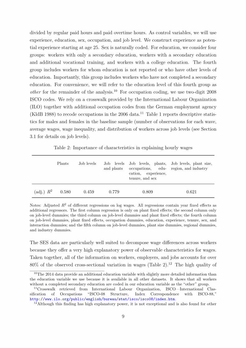
divided by regular paid hours and paid overtime hours. As control variables, we will useexperience, education, sex, occupation, and job level. We construct experience as poten-tial experience starting at age 25. Sex is naturally coded. For education, we consider fourgroups: workers with only a secondary education, workers with a secondary educationand additional vocational training, and workers with a college education. The fourthgroup includes workers for whom education is not reported or who have other levels ofeducation. Importantly, this group includes workers who have not completed a secondaryeducation. For convenience, we will refer to the education level of this fourth group asother for the remainder of the analysis.1010 For occupation coding, we use two-digit 2008ISCO codes. We rely on a crosswalk provided by the International Labour Organization(ILO) together with additional occupation codes from the German employment agency(KldB 1988) to recode occupations in the 2006 data.1111 Table 11 reports descriptive statis-tics for males and females in the baseline sample (number of observations for each wave,average wages, wage inequality, and distribution of workers across job levels (see Section3.13.1 for details on job levels).

Table 2: Importance of characteristics in explaining hourly wages

Plants Job levels Job levelsand plants

Job levels, plants,occupations, edu-cation, experience,tenure, and sex

Job levels, plant size,region, and industry

(adj.) R2 0.580 0.459 0.779 0.809 0.621

Notes: Adjusted R2 of different regressions on log wages. All regressions contain year fixed effects asadditional regressors. The first column regression is only on plant fixed effects; the second column onlyon job-level dummies; the third column on job-level dummies and plant fixed effects; the fourth columnon job-level dummies, plant fixed effects, occupation dummies, education, experience, tenure, sex, andinteraction dummies; and the fifth column on job-level dummies, plant size dummies, regional dummies,and industry dummies.

The SES data are particularly well suited to decompose wage differences across workersbecause they offer a very high explanatory power of observable characteristics for wages.Taken together, all of the information on workers, employers, and jobs accounts for over80% of the observed cross-sectional variation in wages (Table 22).1212 The high quality of

10The 2014 data provide an additional education variable with slightly more detailed information thanthe education variable we use because it is available in all other datasets. It shows that all workerswithout a completed secondary education are coded in our education variable as the “other” group.

11Crosswalk retrieved from International Labour Organization, ISCO—International Clas-sification of Occupations “ISCO-08 Structure, Index Correspondence with ISCO-88,”http://www.ilo.org/public/english/bureau/stat/isco/isco08/index.htmhttp://www.ilo.org/public/english/bureau/stat/isco/isco08/index.htm.

12Although this finding has high explanatory power, it is not exceptional and is also found for other

9

the data is key for delivering this very high degree of statistical determination. Besidesdata quality, the other and economically more important reason for the high explanatorypower is that we observe job levels. Dummies for five job levels alone account for morethan 45% of cross-sectional wage variation; adding plant dummies observables accountsfor 78%; and combining job levels with plant characteristics accounts for 62% of wagevariation.1313 We corroborate our findings on the high explanatory power of job levels forwages in US NCS data in Appendix AA. Given its high explanatory power for wages, wediscuss the job-level variable in more detail next.

3.1 Job levels

A key distinction of the SES data from many other data sources is that they provideinformation on workers’ job levels.1414 Job levels are assigned based on a job’s complexity,autonomy, and responsibility in the execution of the job’s tasks. Complexity of taskexecution relates to the minimum skill and education requirements that a worker willneed to execute the job’s tasks. As a minimum requirement, it does not rule out thatworkers with more skills (human capital) do a job that requires less than their stock ofskills. Autonomy captures how closely a jobholder has to follow a predefined work flowand how much decision-making power is granted in the execution of tasks. Responsibilityrefers to the scale of operations affected by the jobholder’s decisions, i.e., if task executiononly affects one’s own work or also the work of others. Conceptually, we therefore thinkof jobs as being described by two dimensions: on the one hand, by the occupation asdescribing an extensive margin of tasks (which tasks are done), on the other hand, by thejob level as an intensive margin of task execution (how are tasks done). Importantly, joblevels in the data are constructed such that they offer a consistent measure of the intensityof task execution within and across occupations.1515 We therefore follow the key idea of thetask-based approach (Autor et al.Autor et al., 20032003) that wages are determined by executed tasksrather than by the stock of human capital (Acemoglu and AutorAcemoglu and Autor, 20122012). We complementthe task-based perspective by the refined distinction between the extensive margin of taskexecution (occupations) and an intensive margin of task execution (job levels).In the SES data, the statistical office encodes five job levels, job level 1 to 5, but doesnot assign titles. To ease the further discussion, we assign labels to job levels. Thelowest job level is for simple tasks with a clearly defined work flow. These jobs have no

administrative linked employer-employee data (see, for example, Strub et al.Strub et al., 20082008).13Appendix Figure 3030 shows the large wage differences by job level over the entire life cycle in the SES

data.14The NCS data for the United States also provide job level information. See Appendix AA for details.15The BLS job-leveling guide describes in detail the job-leveling approach for the US NCS data

(US Bureau of Labor StatisticsUS Bureau of Labor Statistics, 20132013).

10

minimum skill requirements so that they can be done by untrained workers (untrained,UT). Specifically, the minimum skill requirements are set so that tasks do not requireparticular training (such as an apprenticeship) and can be learned on the job in lessthan three months. The second job level covers tasks that require some occupationalexperience but no completed occupational training such as an apprenticeship (trained,TR). Tasks performed at this job level can typically be learned on the job in less thantwo years. Task execution on the lowest two job levels follows clearly defined rules andprocedures so that workers do not undertake any decisions independently but follow aclearly defined work flow. Only from the third job level onward do employees have somediscretion regarding their work flow. Jobs at the third job level (assistants, AS) areso complex that they require a completed occupational training (apprenticeship) and, inaddition, occupational experience. At this job level, jobholders prepare decisions or makedecisions within narrowly defined parameters. Examples would be tradespeople, juniorclerks, or salespeople who decide on everyday business transactions (e.g., sales). Yet, thetask execution on these jobs does not include responsibility for the work of others or deci-sions that affect the work of others like strategic business decisions. The fourth job levelis assigned to jobs with tasks that typically require both specialized (academic or occupa-tional) training and experience (professionals, PR). Importantly, these jobs require thattasks be performed independently and are associated with substantial decision-makingpower over cases, transactions, or work flow organization. The complex tasks assigned tothese jobs typically require autonomy in organizing the work flow to successfully completethe job tasks. Holders of professional jobs have some decision-making power in regardto the work of others or their decisions affect the work of others; examples would beproduction supervisors, junior lawyers, or heads of administrative offices. The fifth joblevel is managers and supervisors (management, MA). The task execution on these jobsis primarily decision making and dealing with complex cases that require high levels ofautonomy and often come with substantial responsibility regarding the work of others,e.g., senior lawyers, medical doctors, and senior researchers. A high job level does not,however, necessarily require the existence of workers at lower job levels at the plant orin the production process. For example, all jobs in research will be classified in the twohighest job levels because of their complexity, autonomy, and responsibility. The factthat job levels do not require subordinate hierarchies at the plant distinguishes job levelsfrom theories of production hierarchies as in Garicano and Rossi-HansbergGaricano and Rossi-Hansberg (20062006).The discussion already hints at several links between job levels, occupations, and jobtasks. Appendix BB provides a detailed discussion of how job levels differ from occupationclassifications and how the task execution encoded in job levels relates to the task-basedapproach (Autor et al.Autor et al., 20032003). We also demonstrate that job levels can be directly con-

11

structed from questions on skill requirements, autonomy, and responsibility in survey datahighlighting a distinction to tournament models of career progression (Lazear and RosenLazear and Rosen,19811981). We summarize the key points of the discussion here and refer the interested readerto Appendix BB for further details. We discuss the relationship of job levels to educationin Section 5.25.2 when we discuss the implications of our empirical results for returns toeducation.With respect to occupations, we document in Section B.1B.1 that at the level of two-digitoccupations, more than half of the occupations have at least 10% of workers on threedifferent job levels and these results remain almost unaffected if we use the finest avail-able five-digit occupation codes. Using the five-digit occupation codes, we also demon-strate that the encoded complexity classification of the modern occupational classifi-cation, KldB2010, does not account for the differences in job levels. The task-basedapproach by Autor et al.Autor et al. (20032003) groups occupations based on task descriptions so thatby construction their approach cannot account for any within-occupation dispersion. Wefind that in our data average job levels account for 73% of average occupational wagedifferences, while a task-based regression accounts for only half of the dispersion. In-cluding job levels and task-based measures in the regression renders most task measuresinsignificant and lets them explain little variation in a statistical sense. In Section B.4B.4,we address the concern that job levels have high explanatory power for wages as theyjust encode wage levels within firms and ideas closely related to the tournament theoryin Lazear and RosenLazear and Rosen (19811981). We demonstrate that this is not the case, as job levelsconstructed from survey questions on skill requirements, autonomy, and responsibilityin task execution account for 44% of wage variation very similar to job levels in theSES data. We also corroborate this finding in US NCS data in Appendix AA. The factthat job levels can be derived independent of the wage structure has also been shownin case studies (Dohmen et al.Dohmen et al., 20042004). In summary, we conclude that job levels have aneconomic content similar to occupations by describing task execution of a job. Whileoccupations describe which tasks have to be done on the job, an extensive margin of taskexecution, job levels describe how these tasks have to be executed, an intensive marginof task execution.

4 The life cycle of wage growth and wage inequality

This section explores how much plant, job, and worker characteristics account for life-cycle wage growth and the rise in wage inequality over the life cycle. It builds on thestrength of the data that job, worker, and plant characteristics account for more than

12

80% of wage variation in the cross section (Table 22). In the first part, we describe themethodology of our decomposition approach and discuss identification. In the secondstep, we discuss results and interpret them.

4.1 Methodology

One challenge for the decomposition of life-cycle wage dynamics is that unobserved in-dividual characteristics could jointly affect wages and the career progression of workers.A simple OLS estimate of wages on job levels would then be inflated because more ableworkers obtain higher wages at any job and are also more likely to end up at higherjob levels. Such unobserved worker heterogeneity as the driver of career dynamics isthe focus of the seminal work by WaldmanWaldman (19841984) and Gibbons and WaldmanGibbons and Waldman (20062006).We deal with the challenge of unobserved heterogeneity by relying on two different ap-proaches. First, we estimate a synthetic panel specification that exploits the fact thataggregating microdata to the cohort level creates a panel structure so that we can controlfor unobserved heterogeneity in the decomposition (see DeatonDeaton, 19851985; VerbeekVerbeek, 20082008, foran overview of the method).1616 The aggregation to the cohort level further mitigates theconcern of biased estimates as the identification stems only from the variation in the jobcomposition across cohorts. As a second approach, we estimate the effects of job levels onwages using a shift-share type instrument (BartikBartik, 19931993). We discuss the synthetic panelapproach as our baseline approach next and relegate the discussion of the instrumentalvariable using a shift-share instrument approach to Appendix CC.We start from the following empirical model of log wages wipt of individual i working atplant p at time t

wipt = γi + ζpt + βJJipt + βIIipt + ϵipt, (1)

where Jipt is the characteristics of the job of individual i at plant p at time t, Iipt is thecharacteristics of the individual itself, γi is a worker fixed effect, and ζpt is a plant-yeareffect. The individual component, βIIipt, captures the wage effect of worker characteristicscomprising the measures of a worker’s human capital, education and experience, that weinclude as education and gender-specific age dummies.1717 The job component, βJJipt,captures the characteristics of a job. We use dummies for two-digit occupations and fivejob-level dummies.

16Appendix D.5D.5 considers a specification in which we do not control for individual fixed effects.17We group ages using three-year windows to identify cohort effects later on, given the four-year

distance between the three survey waves.

13

To control for plant-year effects, we demean all variables at the plant level (year by year):

wit := wipt − w.pt = γi + βJ Jit + βI Iit + ϵit, (2)

where Xit denotes the difference between variable Xipt for worker i and its average X.pt atthe plant where this worker is working. We explain below how we construct the estimateof the plant component, ζpt. To control for individual-specific fixed effects, we rely onpanel regressions for synthetic cohorts. We define cohorts based on workers’ sex, birthyear, and regional information (north-south-east-west),1818 and we aggregate variables tothe cohort level to obtain

ˆwct = ˆγc + βJˆJct + βI

ˆIct + ˆϵct, (3)

where ˆXct denotes the average of Xit within cohort c. This means that we estimate thecoefficients of interest, β, from aggregate cohort data instead of from individual data.This allows us to use fixed effects OLS to obtain unbiased estimates βJ and βI fromequation (33) even in the presence of unobserved heterogeneity at the individual level thatmight lead to cohorts differing in their unobserved average fixed effect ˆγc. Hence, werely on the key idea of DeatonDeaton’s (19851985) synthetic panel estimator and use between-groupvariation in outcomes and observables for identification of the coefficients of interest.Using the coefficient estimates βJ and βI , we construct the estimate for the plant compo-nent ζpt. The plant component represents the residual plant-level wage after accountingfor worker and job observables. It is given by

ζpt = w.pt − βJJ.pt − βII.pt. (4)

This construction implies that the plant component corrects the average wage at a plantfor differences in organizational structure and workforce composition by removing theaverage individual and job components across plants. Hence, a high-wage plant is aplant that pays on average more than other plants after accounting for worker and jobobservables at that plant. Unlike Abowd et al.Abowd et al. (19991999), we do not have individual-levelpanel information to identify residual worker fixed effects so that the average worker effectat a plant is not separately identified from the plant effect, but the individual and jobcomponent are consistently estimated. If there is no assortative matching in unobservedplant and worker heterogeneity, then the plant component is consistently estimated. If

18The annual gross migration rate between German states in the past 30 years is low and has beenroughly 1.3% per year; see Wanderungsstatistik of the Statistisches Bundesamt. More than a third ofthis migration is between states of the same region.

14

matching is positively (negatively) assortative, the plant effect tends to be positively(negatively) biased.1919

The minimum observations across cohort-year cells is 415, the maximum is 8,383, andthe median is 3,461. Identifying assumptions for our regression are that all coefficients,in particular the pure experience effects on life cycles (captured by βI), are stable acrosscohorts and that regressors have overlapping support across cohorts.To understand the identifying variation that we exploit, recall that we have first de-meaned the data at the plant-year level and, hence, have taken out region-year effectsas well. Second, we have taken out cohort effects in the estimation. Therefore, we donot use differences across cohorts or common time trends of all cohorts in a region foridentification, but instead exploit different time variation across cohorts for identifyingβJ and βI . In other words, we exploit how wages and (job) characteristics evolve overtime within a cohort while simultaneously controlling for variations that affect all cohortsin a region.An example for the type of variation we use is the entry of a new plant into a region,for which this plant has an atypical organizational structure. If this has more of aneffect on the job characteristics of worker cohorts that are young at the time of entryat that plant relative to those of older cohorts, we get a variation that identifies thejob effect. Such an effect should be strongest around the entry date of a plant becauseyounger workers are more mobile and hence more likely to exploit new job opportunities.Another example would be (regional) business cycles with heterogeneous impacts oncohorts. More generally speaking, identification comes from changes in the structure ofjob opportunities within a region over time, but since this affects different age groupsdifferently, the variation is not captured by the region-year effect.In our baseline, we use the entire variation in the organizational structure across cohortsto identify effects. We also consider an instrumental variable approach that tackles theconcern over endogeneity of the organizational structure to changes in worker charac-teristics over time. For this purpose, we construct a Bartik-style instrument (BartikBartik,19931993): First, we construct for a cell defined by age, gender, region, and industry theaverage share of workers of a given industry who work at a given job level, averagingover all sample waves. We do the same for occupations. We then interact these shareswith the aggregate (country-wide) changes in employment for all industries and years toobtain predicted employment shares in each occupation and job level for each cohort andsurvey year. Finally, we use these constructed shares to instrument the actual shares

19The estimate by Card et al.Card et al. (20132013) for Germany is based on the Abowd et al.Abowd et al. (19991999) approach thatis not directly comparable to our results as it does not control for the organizational structure at the firm.They find a modest positive contribution to cross-sectional wage inequality from assortative matching.

15

of workers within a cohort across job levels. Estimation results using this IV approachcorroborate qualitatively and quantiatively our baseline results based on the synthetic-cohort approach. We relegate the discussion of the IV results therefore to Appendix CC.Given its simpler interpretability and favorable small sample properties, we use the OLSestimation with cohort fixed effects as our baseline approach.

4.2 Wage growth

In the first step, we decompose average wage growth over the life cycle. The estimatedworker component, βIIipt, and job component, βJJipt, include worker and job charac-teristics that can still contain cohort effects, we therefore remove these effects from theestimated components by regressing them on a full set of cohort and age dummies. Wereport the coefficients on the age dummies as our life-cycle profiles and always normalizethe log wage components of a 25-year-old worker to zero. We decompose the wage growthof male and female workers separately because these decompositions show very distinctpatterns. We first look at males and discuss female workers in a second step. We discussdifferences between males and females in Section 55 when discussing the implications ofour results for the evolution of the gender pay gap.

4.2.1 Males

Figure 1: Wage and job component decomposition (males)

0.1

.2.3

.4.5

25 30 35 40 45 50 55

Total Individual component

Plant component Job component

(a) Wage

0.1

.2.3

25 30 35 40 45 50 55

Job component Job−level component

Occupation component

(b) Job component

Notes: Left panel: Decomposition of log wage differences by age relative to age 25 for male workers.The dashed line corresponds to the individual, the dotted line to the plant, and the dash-dotted line tothe job component; the solid line (total) equals the sum over the three components. The horizontal axisshows age, and the vertical axis shows the log wage difference. Right panel: Decomposition of the jobcomponent (solid line) into the contribution of occupations (dotted) and job levels (dashed).

Figure 11(a) reports the decomposition of mean log wages for men. On average, wages grow

16

by approximately 45 log points over the life cycle and we find that the job component,climbing the career ladder, accounts for more than 50% of wage growth. Moving tobetter-paying plants over the life cycle, the plant component, contributes approximately20% to life-cycle wage growth, but it is particularly important after labor market entry(Topel and WardTopel and Ward, 19921992; Bagger et al.Bagger et al., 20142014). The remainder, the individual component,captures a pure experience effect.The fact that climbing the career ladder is the most important component of wage growthcan be seen when looking at the decomposition of the job component (Figure 11(b)). Wefind that promotions across job levels, the intensive margin of task execution, accountsfor virtually all of the wage growth and that movements across occupations, the extensivemargin of tasks, contribute slightly negatively to wage growth once we control for job lev-els. In turn, most of the life-cycle wage growth is accounted for by workers taking on jobsat higher job levels, meaning jobs with increasing degrees of responsibility, complexity,and autonomy over the course of their careers.

4.2.2 Females

Figure 2: Decomposition of wage and job component (females)

0.0

5.1

.15

.2.2

5

25 30 35 40 45 50 55

Total Individual component

Plant component Job component

(a) Wage

0.0

5.1

.15

.2

25 30 35 40 45 50 55

Job component Job−level component

Occupation component

(b) Job component

Notes: Decomposition of average wages of female workers; otherwise, see Figure 11.

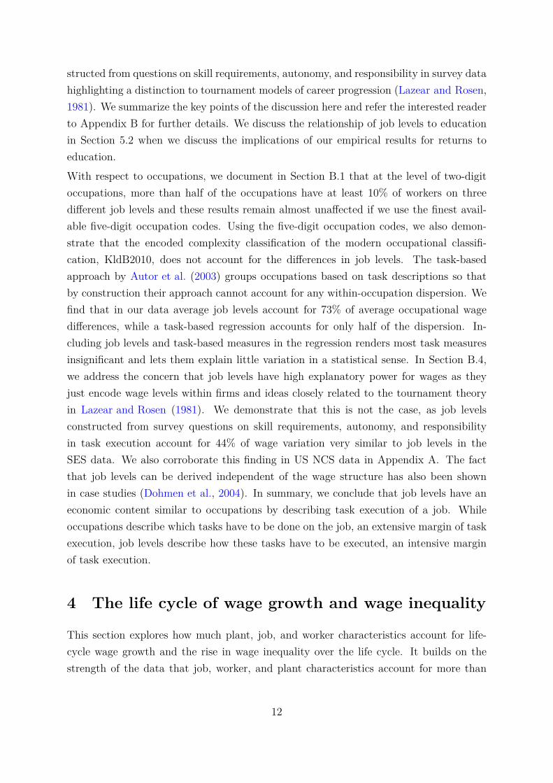
The average wages of females are lower and grow less over the life cycle relative to malewages. Female wages grow by only 25 log points compared to 45 log points for males. Ourdecomposition in Figure 22(a) shows that a substantial part of this difference is accountedfor by the smaller increase in the job component, in particular, a slower progression ofwomen on the career ladder. The job component still accounts for the lion’s share (18log points), but compared to males (25 log points), the average female job componentis substantially flatter. The reason is that between ages 30 and 45, there is hardly any

17

growth in the job component for females. It starts to increase slightly again only after age45. Unlike for men, we find for women that a substantial part of the increase in the jobcomponent stems from the occupation component, which accounts for almost 5 log pointsof females’ wage growth (Figure 22(b)). The individual component for females accountsin relative terms for slightly more of the total growth than for men (30% versus 25%).Interestingly, the plant component shows a decreasing profile for females after age 30.One reason could be that the nonwage aspects of a plant, such as its location or workingtime arrangements, play more important roles for females than for males at this stage ofthe life cycle.2020 As we document in Section 5.35.3, the plant component is correlated withthe organizational structure of plants in terms of job levels. Plants with a high plantcomponent offer on average more jobs at top job levels. The decomposition shows that,over time, fewer and fewer females work at these plants.In summary, these results demonstrate that most of the life-cycle wage growth for malesand females is accounted for by changes in how tasks are executed (job levels) ratherthan which tasks are executed (occupations). We find that on average wage growth is theresult of workers climbing the career ladder to jobs that are more complex and requirejobholders to take more autonomy and responsibility. Next, we show that not all workersfollow the same career path so that wage inequality rises over the life cycle.

4.3 Wage inequality

Wages do not only grow over the life cycle but they also become more unequal as workersage. The high degree of statistical determination in our data allows us to provide a fine-grained decomposition of the drivers of this rising wage inequality. Figure 33 shows thevariance of log wages for males and females by age from the raw data. We find the typicalpattern of an almost linear increase in the cross-sectional variance for males. For females,the pattern is similar until their early 30s and flat thereafter. We rely on the estimatedjob, worker, and plant components to construct variance and covariance estimates of thejob, individual, and plant component by age and to decompose the life-cycle increase inwage inequality. As for wage growth, we first discuss males, then females.

4.3.1 Males

The variance of log wages for men increases substantially over the life cycle: 11 log pointsover 30 years (15 log points after controlling for cohort effects). Bayer and JuessenBayer and Juessen (20122012)find a comparable number for household wages in the German SOEP data. Heathcote et al.Heathcote et al.

20For Brazil, Morchio and MoserMorchio and Moser (20202020) find an important role of nonwage pay components to accountfor the gender pay gap.

18

Figure 3: Variance of log wages by age (raw data).1

.125

.15

.175

.2.2

25

.25

25 30 35 40 45 50 55

(a) males

.1.1

25

.15

.175

.2.2

25

.25

25 30 35 40 45 50 55

(b) females

Notes: Variance of log wages for males and females. Left panel shows males, right panel shows females.Horizontal axis shows age, and vertical axis log wage variance.

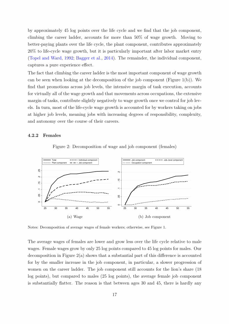
(20102010) report for the United States an increase between 17 and 20 log points over thesame part of working life. Existing microdata based on cross-sectional regressions typi-cally account for about 30% of wage inequality by observables and leave the largest partof wage inequality unexplained. Consequently, the literature interprets the largest partof the increase in wage inequality by age as the result of idiosyncratic risk captured bya stochastic process. This is the typical approach in a wide range of models includingthe large class of microfounded models of consumption-savings behavior (HuggettHuggett, 19931993;AiyagariAiyagari, 19941994).In Figure 44(a), we display the decomposition of life-cycle wage dispersion.2121 We find thatthe variance of log wages of workers increases from roughly 10 log points to 25 log points.The variance of the plant component contributes to the level of wage dispersion with 6to 7 log points but is mostly flat over the life cycle. The job component, by contrast,shows an 11 log point increase in its variance, from 6 to 17 log points. Put differently,two-thirds of the total increase in wage variance is accounted for by workers becomingincreasingly different in the type of jobs they hold. As for average wages, the job levelis the main driving variable (not displayed). The variance of the individual componentis virtually zero. Education itself has a negligible direct effect on wage differences acrossworkers.Two remaining components are unreported in Figure 44(a): the variance of what is notaccounted for by observables (residual wage dispersion) and the sum of all covarianceterms of observables. Figure 44(b) shows the covariance terms by splitting the covariance

21Here, we control for cohort effects and the profile becomes steeper relative to the raw data in Figure33.

19

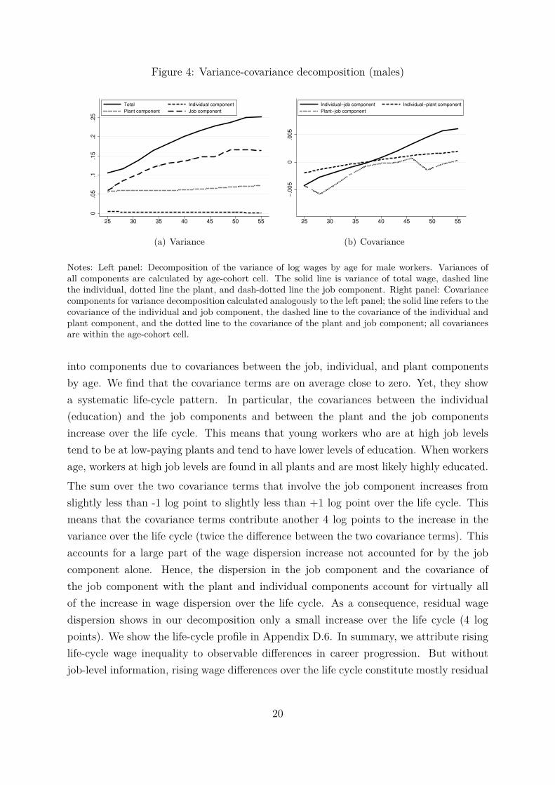
Figure 4: Variance-covariance decomposition (males)0

.05

.1.1

5.2

.25

25 30 35 40 45 50 55

Total Individual component

Plant component Job component

(a) Variance

−.0

05

0.0

05

25 30 35 40 45 50 55

Individual−job component Individual−plant component

Plant−job component

(b) Covariance

Notes: Left panel: Decomposition of the variance of log wages by age for male workers. Variances ofall components are calculated by age-cohort cell. The solid line is variance of total wage, dashed linethe individual, dotted line the plant, and dash-dotted line the job component. Right panel: Covariancecomponents for variance decomposition calculated analogously to the left panel; the solid line refers to thecovariance of the individual and job component, the dashed line to the covariance of the individual andplant component, and the dotted line to the covariance of the plant and job component; all covariancesare within the age-cohort cell.

into components due to covariances between the job, individual, and plant componentsby age. We find that the covariance terms are on average close to zero. Yet, they showa systematic life-cycle pattern. In particular, the covariances between the individual(education) and the job components and between the plant and the job componentsincrease over the life cycle. This means that young workers who are at high job levelstend to be at low-paying plants and tend to have lower levels of education. When workersage, workers at high job levels are found in all plants and are most likely highly educated.The sum over the two covariance terms that involve the job component increases fromslightly less than -1 log point to slightly less than +1 log point over the life cycle. Thismeans that the covariance terms contribute another 4 log points to the increase in thevariance over the life cycle (twice the difference between the two covariance terms). Thisaccounts for a large part of the wage dispersion increase not accounted for by the jobcomponent alone. Hence, the dispersion in the job component and the covariance ofthe job component with the plant and individual components account for virtually allof the increase in wage dispersion over the life cycle. As a consequence, residual wagedispersion shows in our decomposition only a small increase over the life cycle (4 log

points). We show the life-cycle profile in Appendix D.6D.6. In summary, we attribute risinglife-cycle wage inequality to observable differences in career progression. But withoutjob-level information, rising wage differences over the life cycle constitute mostly residual

20

wage inequality and get attributed to persistent shocks to wages. In short, our resultssuggest that differential career progression is a key source of rising wage inequality overthe life cycle and we provide suggestive evidence in Section 5.45.4 that career progressionstill contains a substantial luck component.

4.3.2 Females

We have seen that women have a flatter average job-level component than men after age30. This result also has implications for the evolution of life-cycle wage inequality amongwomen. Their wage dispersion grows less by age (Figure 55(a)). In particular, the increaseaccounted for by job-level dispersion is much smaller for women than for men and levelsoff after age 30. Still, the life-cycle profile of the job component accounts for over two-thirds of the 12 log point increase in wage dispersion over the working life of females(compared to a 15 log point increase for the variance of males). For females, we alsofind a virtually flat life-cycle profile in the plant component (Figure 55(a)) and residualcomponent (Figure 2828 in Appendix D.6D.6). At the same time, the job-plant covarianceprofile is even steeper for women than for men (Figure 55(b)). Those women who end upat high job levels at age 50 work in high-paying plants. Yet, as will be shown in Figure88 in Section 55, we know that later in their working life, fewer women tend to work inhigh-paying plants than at age 30. Adding all terms related to the job component as inthe decomposition for males, we also find that virtually all of the life-cycle increase inwage inequality is accounted for by the job component.

Figure 5: Variance-covariance decomposition (females)

0.0

5.1

.15

.2

25 30 35 40 45 50 55

Total Individual component

Plant component Job component

(a) Variance

−.0

1−

.00

50

.00

5

25 30 35 40 45 50 55

Individual−job component Individual−plant component

Plant−job component

(b) Covariance

Notes: Decomposition of the variance of wages of female workers; otherwise, see Figure 44.

Our decompositions of life-cycle wage growth and life-cycle wage inequality assign a keyrole to career ladder dynamics, i.e., workers progressing differentially across job levels

21

as they age. We find a tight link between wages and changes in workers’ job levelsdescribing the autonomy, complexity, and responsibility in task execution on the job. Weconceptualized these differences in job levels within and across occupations as variationof the intensive margin of task execution as distinct from occupations as the extensivemargin of tasks. Except for the average wage growth of females in the second half oftheir working life, we always find a dominant role within the estimated job componentfor changing job levels in accounting for life-cycle wage dynamics. We therefore explorein the next step career ladder dynamics in more detail.

4.4 Labor market mobility and career dynamics

In this section, we explore career ladder dynamics and how important labor marketmobility and employer switching are for career progression. Importantly, we do notexplore the complex reasons why workers move to different employers but only explorethe consequences of such employer switching.In a first step, we still rely on SES data to explore in Figure 66 how long workers stay withtheir employers at different stages of the career ladder. Specifically, the figure shows byhow much tenure increases (in years) from one five-year age group to the next five-yearage group, at different job levels. If all workers stayed with their employer all the time,the increase between age groups would be five. We find that the tenure increase by ageis larger at higher job levels and that the increase accelerates over workers’ careers. Thesteeper increase across job levels and age already suggests that many workers climb thecareer ladder while staying with their employer.To further address the question of the importance of employer switching for career dy-namics, we rely on German panel data from the SOEP, which allows us to follow individ-ual workers over time. The SOEP data provide information on individual labor marketsituations together with workers’ demographics and income (Goebel et al.Goebel et al., 20192019). SeeAppendix EE for further data details. The data cover the period from 1984 to 2015. Aspart of these data, the SOEP collects information on job levels similar to the coding inthe SES data but not directly comparable. The limitation of the coding in the SOEP isthat it is based on ideas from the sociological literature (Hoffmeyer-ZlotnikHoffmeyer-Zlotnik, 20032003), andas such it loads more heavily on education and therefore tends to bias downward workermobility across job levels.2222 With this caveat in mind, we use the job level from theSOEP data to explore worker mobility and career progression.To align the SOEP sample and the SES sample, we keep workers ages 25 to 55 working

22Conditional on the job level, the SOEP data show quantitatively similar wage differences betweenjob-level age profiles, as found in the SES data. We provide details in Appendix EE.

22

Figure 6: Tenure increase by age and job level

01

23

4

Untrained Trained Assistant Professional Management

25

−2

93

0−

34

35

−3

94

0−

44

45

−4

95

0+

25

−2

93

0−

34

35

−3

94

0−

44

45

−4

95

0+

25

−2

93

0−

34

35

−3

94

0−

44

45

−4

95

0+

25

−2

93

0−

34

35

−3

94

0−

44

45

−4

95

0+

25

−2

93

0−

34

35

−3

94

0−

44

45

−4

95

0+

Notes: The figure displays the average additional years of tenure of an age group relative to the precedingone by job level. Averages over all sample years are shown for both males and females. For 25- to 29-year-olds, the figure shows the average number of years of tenure in the group.

at employers with 10 or more employees. We drop self-employed workers, apprentices,military personnel, and public service workers. We drop all observations with missinginformation on job level, industry, education, occupation, or number of employees at theiremployer. Data are at an annual frequency, and we explain below how we define labormarket mobility events.In the first step, we construct life-cycle profiles of promotion and demotion rates. Promo-tions (demotions) are naturally coded as a change in the job level from the current surveydate to a higher (lower) job level at the next survey date. Figure 77 reports estimatedlife-cycle profiles of annual promotion and demotion rates for males and females. We finddeclining promotion rates for both genders during the working life, in line with a concavewage profile. Males show higher promotion rates in the first part of the life cycle. Atage 55, the levels of promotion rates for males and females have converged. Demotionrates are strikingly constant over the entire working life, and levels are very close betweenmales and females. For both genders, demotion rates are substantially below promotionrates at the beginning of working life. In the late 40s, the levels of promotion and demo-tion rates roughly converge, implying no further net career progression. In Appendix EE,we compare net promotion rates, promotion rates minus demotion rates, for males andfemales and show that net promotion rates diverge most strongly between ages 25 and35 (Figure 3131). We return to these differences in promotion rates from SOEP data when

23

Figure 7: Promotion and demotion rates by age2

46

81

0

25 30 35 40 45 50 55

promotions demotions

(a) Males

24

68

10

25 30 35 40 45 50 55

promotions demotions

(b) Females

Notes: Annual promotion and demotion rates by age for males and females based on SOEP data, years1984-2015. All rates are shown in percentages. The left panel shows promotion and demotion rates formales, the right panel the promotion and demotion rates for females.

discussing the gender pay gap in Section 5.15.1.To explore how labor market transitions are associated with career dynamics, we definefour mobility events. We assign an “employer-change” event to a worker-year observationif the person is employed at both survey dates but is employed for less than one year withthe current employer at the second date. We define a transition through nonemploymentif a worker is nonemployed at the first survey date but employed at the second surveydate. We assign an occupation change if workers answer positively to the question ofwhether “there has been a change in their job” and the recorded occupation changed.2323

Finally, we define the group of stayers as those workers who neither change employers norgo through nonemployment. Using these mobility definitions, we ask whether promotionsand demotions happen with the same employer or whether labor market mobility is a keydriver of promotion and demotion dynamics.Table 33 shows the share of all promotions and all demotions accounted for by stayers andmovers. We find that more than 70% of promotions happen for workers who stay withtheir employer, while less than 30% of all promotions are associated with an employerchange. For demotions, we find a similar distribution: about 60% of demotions happenat the same employer, while 40% involve a change of employers.Table 44 changes perspectives by reporting the distribution of promotions, demotions, andlateral moves conditional on employer changes, transitions through nonemployment, and

23We condition on the information of job change to reduce measurement error in the occupation codes.It is well known that occupation codes are prone to be recorded with error so that occupational changesare too prevalent in household survey data (Kambourov and ManovskiiKambourov and Manovskii, 20132013).

24

Table 3: Promotions and demotions for stayers and movers

employer change (%) stayer (%)

promotion 28.6 71.4

no change 11.8 88.2

demotion 38.1 61.9

Notes: Shares of all promotions and demotions that happen for workers staying with the same employersduring the year (column stayer) and workers changing employers (column employer change). Each rowsums to 100%.

Table 4: Promotions and demotions for labor market transitions

employer non- occupationstayer (%) average (%)change (%) employment (%) change (%)

demotion 6.6 10.7 11.0 2.2 3.0

no change 84.5 77.3 75.6 93.6 92.0

promotion 9.0 12.0 13.5 4.2 5.0

net promotion 2.4 1.3 2.5 2.0 2.0

Notes: Promotions and demotions for different mobility events (see text for details). Each column showsa mobility event and the share of workers conditional on this mobility event who have a promotion ordemotion. The row net promotion reports the difference between promotion and demotion rates for eachmobility event. The first three rows (excluding net promotions) of each column sum to 100%.

occupation changes. We report stayers and the average across all workers as a reference.The results support the idea that labor market mobility implies more movement onthe career ladder. We find that both employer changers and workers who go throughnonemployment exhibit more mobility on the career ladder compared to job stayers.We find that 9% of all employer changes involve a promotion, in line with the ideathat workers move to another employer to climb the career ladder. Yet, we also findthat 7% of employer changes are associated with a demotion. On net, workers with anemployer change have a 20% higher than average net probability of career progression(net promotion = promotion − demotion rates). Perhaps surprisingly, we also find that12% of nonemployment transitions involve a promotion. The promotion in this case isrelative to the last job before nonemployment; that is, here we look for at least two-yearchanges in job levels. Since 11% of all nonemployment transitions involve a demotion,on net, workers after a nonemployment spell experience slower career progression than

25

any other group. Their annualized net promotion rate is therefore at least 70% lowerthan the rate of the average worker. We observe the strongest career progression foroccupation changers, who have a 25% higher net promotion rate than the average worker.Notwithstanding, a change in occupation does not involve a promotion for 87% of alloccupation changers (11% demotions, 76% lateral moves). Looking at job stayers, wefind that there is substantially less mobility on the career ladder: only 4% of workersmove up the career ladder each year, and 2% move down. Stayers account for the largemajority of workers and, therefore, largely determine average promotion and demotionrates in the German labor market (Table 33).

4.5 Sensitivity and extensions

We provide an extensive sensitivity analysis of our results from this section in AppendixDD. In particular, we explore several extensions to our baseline specification from equation(33). In a first step (Section D.1D.1), we explore heterogeneity in the job component of wagesacross worker groups. We explore differences for workers covered by collective bargaining,workers working full-time, and workers working in large plants. In summary, we find thatthe importance of jobs in accounting for wage dynamics increases for workers not coveredby collective bargaining and decreases in large plants. Results for wage growth are verysimilar for full-time male workers, and the effect becomes slightly lower for female workers.For the increase in wage dispersion, we find again that the job component becomesmore important for workers not covered by collective bargaining and less important inlarge plants. The contribution to increasing wage dispersion for full-time workers isslightly lower than in the baseline for both male and female workers. We also explorethe sensitivity of our results when we include public employers and publicly controlledfirms. When including public employers, we find a 30% larger job component for femalewage growth over the life cycle. This finding suggests that public employers offer moreopportunity for female career dynamics, in line with over 60% of employees being femaleat these employers. Overall, we find that the key findings on the importance of the jobcomponent are robust across specifications and sample selections. We relegate furtherdetails and discussion to Appendix DD.In a second step, we explore more flexible specifications to equation (33) where we allow re-turns to experience to be education-specific (Section D.2D.2) or occupation-specific (SectionD.3D.3). We also include employer tenure as an additional component to the wage equation(Section D.4D.4). We find the key result of the importance of career ladder dynamics forwage dynamics to be robust. In the decomposition, we attribute the flexible experienceprofiles to the individual components and attribute tenure to the job component because

26

tenure is related to a worker’s career progression. We find that more flexible experienceprofiles hardly affect the results. Most notably, we find that with education-specific expe-rience profiles, plant components increase in their contribution to wage growth, whereaswith occupation-specific experience profiles, the contribution of the job component tothe increase in wage inequality declines but still accounts for the largest part of all com-ponents. When including employer tenure, we find the most notable change is that thecontribution of the job component to wage growth increases further. These more flexi-ble specifications do not provide any indication that job components are systematicallyinflated in our more restricted setup.Finally, we estimate in Section D.5D.5 the regression in equation (33) by pooled OLS usingcohort fixed effects only, but we do not control for individual fixed effects. We find thatthe result of the job component being the key driver of wage dynamics also holds underthis specification, but results also suggest that there is a substantial omitted variable biasif we do not control for individual fixed effects. In that sense, the results support ourapproach based on a synthetic panel approach.

5 A new perspective on wage dynamics

Our decomposition of life-cycle wage dynamics attribute job levels a pivotal role in ac-counting for wage growth and rising wage dispersion over the life cycle. This sectionbuilds on this key finding to revisit stylized facts on wage dynamics and offers a newperspective on these facts through the lens of career ladder dynamics. Instrumental forthis interpretation is the very high explanatory power of observables and in particularthe large contribution of job levels in accounting for wage dynamics. We revisit as styl-ized wage facts the gender pay gap, returns to education, employer-wage differences, andreturns to seniority but we think that the career ladder perspective applies much morebroadly and can provide additional guidance for refining theories of wage and workerdynamics in the future.For the gender wage gap, we document that it is intimately tied to a widening in job-leveldifferences across gender. In a sense, the gender wage gap is largely a gender promotiongap, echoing findings of Bronson and ThoursieBronson and Thoursie (20182018). Second, we discuss how differencesin promotion patterns can be seen as the main vehicle in generating returns to education.In our data, there is very little return to education absent promotions, but more educatedworkers are much more likely to climb the career ladder. When we drop controls for joblevels, we find that the career ladder dynamics are picked up by substantial returns toeducation. Third, we explore employer-wage differences that have been emphasized as

27

important drivers of the secular rise in German wage inequality (Card et al.Card et al., 20132013). Wedocument that between-employer wage differences can be traced back to differences inorganizational structures across employers. Such organizational differences are in ourdecomposition not part of the employer component but captured by the job component.We demonstrate that once we drop controls for job composition, we find a much larger rolefor employer differences in accounting for life-cycle wage dynamics. Fourth, we explore therelationship between progression on the career ladder and returns to seniority. Returns toseniority have recently been studied by Buhai et al.Buhai et al. (20142014). Corroborating an importantrole for seniority, we find that the most senior worker or being relatively high up in thedistribution of seniority compared to coworkers leads to a significant wage premium. Yet,we also show that three-quarters of this wage premium is accounted for by being higherup on the career ladder. At the same time, these returns to seniority add an element ofluck to career progression as the worker herself cannot fully control her relative senioritywithin a plant, but the relative seniority is a result of the hiring/separation decision ofthe plant and of other workers.

5.1 Gender wage gaps

Males and females earn significantly different wages in the German labor market. Atlabor market entry (age 25), females in our sample receive a roughly 7% lower wage thanmales. At age 50, females earn wages that are more than 30% lower than wages for males.As raw averages, these differences still contain occupational and employer differences. Inour wage growth decomposition, we control for these differences and compare in Figure88 the estimated job-level and plant components for males and females from Figures 11and 22. Figure 88(a) compares the estimated job-level components for males and females.The comparison is striking as it highlights how much the career ladder accounts for thewidening of the gender wage gap over the life cycle.Up to age 30, males and females experience a virtually identical increase in the job-levelwage component. After age 30, the career progression of females comes to a halt, whilemales keep on climbing the career ladder for an additional 15 to 20 years. The differentialprogression on the career ladder results in an increasing wage difference between malesand females exceeding 10 log points at the age of 50. Differences in career dynamicsthereby account for almost half of the increase in the gender wage gap over the life cycle.Most of the remaining wage growth difference is accounted for by differences in the plantcomponent. Again, the different patterns for males and females are striking. While malesmove on average to plants that pay better, females after the age of 30 tend to move toplants that pay worse (Figure 88(b)). A detailed investigation of this differential growth

28

Figure 8: Job-level and plant components of males and females

0.0

5.1

.15

.2.2

5.3

log w

age

25 30 35 40 45 50 55

Male job−level component Female job−level component

(a) Job-level component

0.0

5.1

.15

log w

age

25 30 35 40 45 50 55

Male plant component Female plant component

(b) Plant component

Notes: (a) Job-level component from decomposition of mean log wages for males and females. (b) Plantcomponent from decomposition of mean log wages for males and females. Both: Horizontal axis showsage, and vertical axis shows log wage difference.

trend is beyond the scope of this paper but one potential reason could be non-wageaspects of jobs at worse paying employers as argued in Morchio and MoserMorchio and Moser (20202020).The data span nine years, so that the estimated life-cycle pattern also comes from compar-isons across cohorts. Yet, in Section 4.44.4 we documented career ladder dynamics betweenmales and females in SOEP data that support the idea that women do not climb thecareer ladder as much as men. The SOEP data have the advantage over the SES datathat they offer panel data for more than 30 years. In summary, these results supportthe idea in that the gender wage gap largely stems from a gender promotion gap anddifferences in career ladder dynamics (see also Bronson and ThoursieBronson and Thoursie (20182018)).

5.2 Returns to education

To explore the implications of our findings for returns to education, we provide in Table55 a descriptive analysis of the relationship between education, experience, and the careerladder. We report by age groups the shares of workers at different job levels conditioningon workers’ educational attainment. We look at younger workers ages 25 to 35 andolder workers ages 35 to 45. We further separate male and female workers. This simpledescriptive statistic offers three important results.First, we observe a difference between education (human capital) and job levels. Wefind for all age groups that each education group has significant shares of workers (10%)across at least three job levels. Second, education is positively correlated with job levels.Workers with more education are found on higher job levels in line with the higher

29

Table 5: Share of hierarchy levels within formal education and age groups

at ages 25-35 (in %) at ages 35-45 (in %)

Education UT TR AS PR MA UT TR AS PR MA

Males

Secondary 25.6 37.9 26.7 7.8 2.1 18.3 39.7 29.7 9.2 3.0Vocational 5.5 15.7 60.7 15.7 2.5 3.5 12.7 52.4 24.6 6.8College 1.2 2.8 27.5 48.6 19.9 0.4 1.2 13.8 44.9 39.7Other 17.9 28.9 38.3 12.1 2.8 12.8 27.3 36.2 16.4 7.3

Females

Secondary 30.1 31.3 28.0 8.8 1.8 34.9 35.8 21.4 6.2 1.8Vocational 5.7 13.0 64.3 15.2 1.9 6.3 13.7 57.2 19.8 3.0College 1.9 4.6 35.0 40.3 18.1 0.9 2.9 25.1 43.9 27.3Other 20.2 24.2 42.7 10.9 2.0 27.1 25.7 33.8 10.6 2.9

Notes: Relative frequencies across hierarchy groups in percentage points for different age groups. Thetop part of the table shows male workers, the bottom part female workers. Shares sum within age groupsto 100. “Secondary” refers to workers with secondary education but no vocational training. “Vocational”refers to workers with secondary education as well as a vocational degree. “College” refers to all workerswith a university or technical college degree. Workers without reported education are in the “Other”group. Hierarchy groups UT/TR/AS/PR/MA refer to untrained, trained, assistants, professionals, andmanagers, respectively.

complexity of these jobs. Typically, 60% or more of workers with only a secondaryeducation are at the two lowest job levels (UT+TR). For workers with a college education,we find that typically 60% or more are at the two highest job levels (PR+MA). Third,the distribution across job levels shifts up as workers age. For male and female workersacross all education groups, workers in the age group 35 to 45 are more likely to be foundat higher job levels than workers from the younger age group. For college-educated men,the share of workers in management jobs (MA) doubles from 20% to 40% when comparingthe two age groups. This life-cycle profile highlights the difference between education as a(typically) fixed worker characteristic after labor market entry and job levels that changeover the course of the life cycle and the observed correlations suggest that education andexperience help with progression on the career ladder.We provide further evidence that differential career progression is a pivotal driver of re-turns to education by estimating the main wage regressions from equation (33) leavingout job-level information or the job component altogether. As a measure for the returnsto education, we consider the estimated dummy coefficients for college education. Table66 compares the estimated returns to education from three different specifications. Under

30

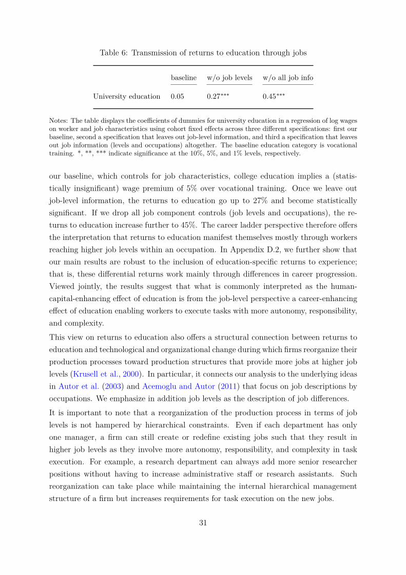
Table 6: Transmission of returns to education through jobs

baseline w/o job levels w/o all job info

University education 0.05 0.27∗∗∗ 0.45∗∗∗

Notes: The table displays the coefficients of dummies for university education in a regression of log wageson worker and job characteristics using cohort fixed effects across three different specifications: first ourbaseline, second a specification that leaves out job-level information, and third a specification that leavesout job information (levels and occupations) altogether. The baseline education category is vocationaltraining. *, **, *** indicate significance at the 10%, 5%, and 1% levels, respectively.

our baseline, which controls for job characteristics, college education implies a (statis-tically insignificant) wage premium of 5% over vocational training. Once we leave outjob-level information, the returns to education go up to 27% and become statisticallysignificant. If we drop all job component controls (job levels and occupations), the re-turns to education increase further to 45%. The career ladder perspective therefore offersthe interpretation that returns to education manifest themselves mostly through workersreaching higher job levels within an occupation. In Appendix D.2D.2, we further show thatour main results are robust to the inclusion of education-specific returns to experience;that is, these differential returns work mainly through differences in career progression.Viewed jointly, the results suggest that what is commonly interpreted as the human-capital-enhancing effect of education is from the job-level perspective a career-enhancingeffect of education enabling workers to execute tasks with more autonomy, responsibility,and complexity.This view on returns to education also offers a structural connection between returns toeducation and technological and organizational change during which firms reorganize theirproduction processes toward production structures that provide more jobs at higher joblevels (Krusell et al.Krusell et al., 20002000). In particular, it connects our analysis to the underlying ideasin Autor et al.Autor et al. (20032003) and Acemoglu and AutorAcemoglu and Autor (20112011) that focus on job descriptions byoccupations. We emphasize in addition job levels as the description of job differences.It is important to note that a reorganization of the production process in terms of joblevels is not hampered by hierarchical constraints. Even if each department has onlyone manager, a firm can still create or redefine existing jobs such that they result inhigher job levels as they involve more autonomy, responsibility, and complexity in taskexecution. For example, a research department can always add more senior researcherpositions without having to increase administrative staff or research assistants. Suchreorganization can take place while maintaining the internal hierarchical managementstructure of a firm but increases requirements for task execution on the new jobs.

31

5.3 Employer wage differences

Our decomposition in Section 44 finds that the plant component accounts for only a smallpart of the increase in wage dispersion over the life cycle. At the same time, recentevidence for Germany and the United States finds employer-wage differences to be a keydriver of increasing wage inequality over time (Card et al.Card et al., 20132013; Song et al.Song et al., 20152015). Atfirst glance, these two pieces of evidence do not seem to align well, but as we will arguenext, they can be reconciled taking a career ladder perspective.We have seen that the plant component and the job component are positively correlatedand increasingly so over a worker’s working life (Figure 44). This implies that the plantcomponent will pick up the organizational structure of plants if we do not control for thejob composition of plants in our life-cycle decomposition.

Figure 9: Shares of employees by job level and plant component

0.1

.2.3

.4.5

Plant Component: Below Median Plant Component: Above Median

UT TR AS PR MA UT TR AS PR MA

Notes: The figure shows the share of workers by job levels in plants with below- or above-medianestimated plant component ζb. The median is defined on a worker basis. 67% of all plants have abelow-median plant component.

The correlation between the plant component and the organizational structure can beseen by considering the distribution of workers across job levels for plants sorted by theestimated plant component ζp (Figure 99). Well-paying plants offer on average more jobs athigher job levels (PR+MA), and only low-paying plants offer a substantial fraction of jobsat the lowest two job levels (UT+TR).2424 This result also aligns with findings of Tåg et al.Tåg et al.(20132013) for Sweden. The plant component in our decomposition captures whether plantspay better at all job levels; that is, the plant component in our baseline decomposition

24Well-paying plants are on average also substantially larger such that the top third of all plants (byplant component of wages) employs 50% of all workers.

32

is not driven by having a larger share of top-level jobs or high-wage occupations at theplant. To explore the importance of the job component and job composition for the wagedecomposition, we proceed as before and drop the job component from our regression inequation (33). We then compare to our baseline decomposition the resulting decompositionof wage dynamics when only an individual and a plant component are present.

Figure 10: Decomposition of wage growth and variance of wages by age (males), ignoringjob controls

0.1

.2.3

.4.5

25 30 35 40 45 50 55

Total Individual component

Plant component

(a) wage growth decomposition

0.1

.2.3

individual plant

baseline no job controls

(b) comparison growth contribution

0.0

5.1

.15

.2.2

5

25 30 35 40 45 50 55

Total Individual component

Plant component

(c) wage variance decomposition

0.0

2.0

4.0

6.0

8.1

individual plant

baseline no job controls

(d) comparison variance contribution

Notes: Top panels show the decomposition of male wage growth in the individual and plant components.The bottom panels show the corresponding decomposition of wage variances for males. The left panelsshow the life-cycle profiles when estimating the components without job controls. The right panels com-pare the components at age 55 to the baseline decomposition that includes job controls (job componentsnot shown here).

Figure 1010(a) shows the decomposition of wage growth for males if we drop the job com-ponent. Looking at this decomposition and comparing it to our baseline in Figure 11, wedraw very different conclusions about the sources of life-cycle wage growth. First, we findthat a substantially larger fraction of wages remains unexplained. Note that experienceconstitutes a residual to the decomposition of mean wages, so that we still account for

33

the entire life-cycle wage growth. More importantly, dropping the job component leadsto an estimate of the role of differences between plants for wage growth that is 50% largerthan in our baseline. Figure 1010(b) compares the life-cycle contribution to wage growthby looking at wage components at age 55. When we decompose the increase in wage dis-persion over the life cycle (Figure 1010(c)), we find a qualitatively similar shift in results.Now, the contribution of plants to wage inequality is 20% larger than in the baseline,and both individual and plant differences contribute significantly to the increase in wagedispersion over the life cycle (Figure 1010(d)). Together, the individual and plant compo-nents account for roughly 8 out of the 15 log point increase in the wage variance. Thecovariance between the individual and plant components also contributes to the growthin wage inequality by 2 log points so that the variance of residual wages also accounts fora larger part of the increase in life-cycle wage inequality (not displayed). We get the sameconclusions when conducting the corresponding decomposition for females and thereforerelegate the results for females to Appendix D.7D.7.These results provide some additional conclusions for why employers are important forlife-cycle wage dynamics. They primarily matter not because of their wage-level differ-ences but because of their differences in organizational structure and associated differencesin career opportunities. These differences in organizational structure are correlated withaverage plant wages and get partly picked up by the plant component when organiza-tional structure is unobserved. While we find wage growth and wage dispersion to beunrelated to the plant itself, the organization of the plant in terms of its job structureis likely an important determinant of workers’ decisions about where they want to workbut we have to leave a further investigation of this hypothesis to future research.

5.4 Returns to seniority

Recently, Buhai et al.Buhai et al. (20142014) have shown that the seniority of workers within the firm isan important factor in determining a worker’s wage—beyond plant, occupation, and pureexperience effects. Specifically, Buhai et al.Buhai et al. establish that not only a worker’s own tenurebut also the relative ranking among coworkers determine workers’ wages. Similarly, weknow from Jäger and HeiningJäger and Heining (20162016) that the wages of workers and the probability ofmoving within a plant to better-paid jobs increase if coworkers leave the plant (in theircase, because of death).These findings are also important from a normative point of view because the effect ofcoworker characteristics adds an element of luck to wage dynamics. Although workers canchange employers and coworkers over time, coworker characteristics can still be consideredlargely beyond a worker’s control as it is impossible for a worker to increase seniority

34

by leaving a plant because this would reset the worker’s tenure to zero and would puther at the bottom of the seniority ranking at the new plant. From the career ladderperspective, the natural question that arises is whether the returns to seniority that theliterature finds are mediated through job characteristics or whether they show up as anindependent (residual) factor.To explore this question, we estimate the effect of the seniority ranking within a plantamong a group of peers that might effectively be competitors for career progression. Weconsider two measures of wages. The first measure is the log wage as reported in thedata. The second is the job-level wage, constructed as the wage that is predicted by thecurrent job level of a worker using the coefficient estimates from equation (33). We alsoconsider two measures for the seniority ranking. In the first case, we include a dummyonly for the most experienced worker within each peer group (based on tenure with thefirm). The estimated coefficients quantify a silverback effect—the effect of being the mostexperienced member of the peer group on (job-level) wages. In the second case, we usewhat we refer to as the seniority rank. For the seniority rank, we follow Buhai et al.Buhai et al.(20142014) and construct the distance between ranks as log(Ni + 1 − ri) − log(Ni) where ri

is the seniority rank of worker i within the worker’s peer group and Ni is the numberof members in worker i’s peer group. For example, the most experienced worker withineach peer group has seniority rank ri = 1, and the least experienced worker has ri = Ni.We get that within each peer group, the distance between seniority ranks varies between[− log(Ni), 0]. We restrict the sample to male workers because of the different careerdynamics for females after age 30. We define a worker’s competitive peer group at aplant as the group of workers who are at most five years older than the respective workerand who have the same educational attainment. We construct within each age-educationcell of the plant the silverback dummy and the distance of seniority ranks. We run threesets of regressions: First, we regress log wages on controls for the seniority ranking;second, we swap the actual wage with workers’ job-level wage; and third, we use thedifference between the two as a regressand to determine the residual seniority premium.Table 77 shows the estimated coefficients.On average, we find the silverback effect and seniority rank distance to be statisticallysignificant. The more experienced a worker, the higher his wage. In the first case, consid-ering only the most experienced worker, we find that these workers obtain a statisticallyhighly significant 6.9% wage premium for seniority based on their raw wages. Their job-level-implied wages are also 5.3% higher, and consequently there is only a small senioritypremium of 2.0% left once we control for job levels. For the second case, using the dis-tance between seniority ranks, we also get a highly significant coefficient of 4.4% for rawwages (close to Buhai et al.Buhai et al.’s estimates for Denmark and Portugal) and 3.6% for job-level

35

Table 7: Being the silverback: the effect of experience ranking on job-level wages

Relative experience concept

Silverback effect Seniority rank

Wage measure Raw Job level Residual Raw Job level Residual

More experienced 6.9∗∗∗ 5.3∗∗∗ 2.0∗∗∗ 4.4∗∗∗ 3.6∗∗∗ 1.2∗∗∗

adj. R2 0.70 0.51 0.62 0.70 0.51 0.62N 335,323 335,323 335,323 335,323 335,323 335,323

Notes: The table displays the coefficients of an OLS regression of a log wage measure of a worker(multiplied by 100) on two sets of controls for experience ranking within peer groups of workers. We usethree different wage concepts: first, the raw log hourly wage of the worker; second, the wage predictedby the worker’s Job level; and third (Residual), the difference between the two (i.e., the wage controllingfor a worker’s job level). A worker’s peer group is composed of all workers at the same plant who are atleast as old as, and up to five years older than, the worker and have the same educational attainment.Experience ranking controls are described in the text. The regression sample includes all male workersages 45 to 50. All regressions include a constant, education dummies (coefficients not reported), andplant fixed effects. *, **, *** indicate significance at the 10%, 5%, and 1% levels, respectively.

wages and again a much smaller residual seniority effect. In other words, we find thatseniority affects wages primarily through giving senior coworkers an edge over their peersin being assigned to higher job levels.These seniority effects are also economically significant. The coefficient for the silverbackeffect implies that the job-level wage is 5.3 log points higher if a worker is the mostexperienced worker within his peer group. To put this into perspective, the job-levelcomponent accounts for approximately 25 log points in wage growth for 45- to 50-year-old workers, such that being the silverback of a group increases the job-level wage byroughly 20%. To quantify the effect of the seniority rank, note that the average numberof members within a peer group is 11. Hence, the difference in the job-level wage betweenthe least experienced member and the most experienced member of an average peer groupis 8.6 log points, 30% of the average job-level component at that age. If one views therelative seniority rank in a group of peers as being largely outside the control of a worker,this result suggests an economically significant role of luck in a worker’s life-cycle wagedynamics.

36

6 Conclusions

Why do wages grow and become more unequal as workers age? This paper exploresadministrative and survey microdata from Germany and the United States to answerthis question. We find that career ladder dynamics play a key role for these life-cyclewage dynamics by documenting a key role for job levels in accounting for life-cycle wagegrowth and rising wage inequality at the level of the macroeconomy. We provide empir-ical evidence documenting the economic content of job levels and how they differ fromoccupations and education. Occupations describe the extensive margin of task execution(which tasks are done) while job levels describe the intensive margin of task execution(how are tasks done), in terms of the complexity, autonomy, and responsibility neededto execute a job’s tasks.The main part of the analysis decomposes life-cycle wage dynamics in German admin-istrative data, where we document the key role for career ladder dynamics, changes injob levels over the working life. Career ladder dynamics account for 50% of wage growthand virtually all of the increase in wage dispersion over the life cycle. We also documentthat labor market mobility is associated with career progression but that most steps upand down the career ladder happen with the same employer. We demonstrate that theimportance of job levels in accounting for wage dispersion holds true in German surveydata and administrative survey data for the United States.We exploit the key strength of the data, its high explanatory power for wages, to traceback otherwise residual wage differences to observable characteristics. We discuss howour findings on the importance of the career ladder for life-cycle wage dynamics offer anew, structural perspective on stylized wage facts; specifically, we discuss the gender paygap, returns to education, employer wage differences, and returns to seniority.

37

ReferencesAbowd, J. M., Kramarz, F., and Margolis, D. N. (1999). High wage workers and high

wage firms. Econometrica, 67(2):251–333.

Acemoglu, D. and Autor, D. (2011). Skills, tasks and technologies: Implications foremployment and earnings. In Handbook of Labor Economics, volume 4, pages 1043–1171. Elsevier.

Acemoglu, D. and Autor, D. (2012). What Does Human Capital Do? A Review of Goldinand Katz’s “The Race between Education and Technology”. Journal of EconomicLiterature, 50(2):426–463.

Aiyagari, S. R. (1994). Uninsured idiosyncratic risk and aggregate saving. The QuarterlyJournal of Economics, 109(3):659–684.

Altonji, J. G. and Shakotko, R. A. (1987). Do wages rise with job seniority? Review ofEconomic Studies, 54(3):437–59.

Autor, D. H., Levy, F., and Murnane, R. J. (2003). The skill content of recent tech-nological change: An empirical exploration. The Quarterly Journal of Economics,118(4):1279–1333.

Autor, David, H., Katz, L. F., and Kearney, M. S. (2006). The polarization of the USlabor market. American Economic Review, 96(2):189–194.

Bagger, J., Fontaine, F., Postel-Vinay, F., and Robin, J.-M. (2014). Tenure, experience,human capital, and wages: A tractable equilibrium search model of wage dynamics.American Economic Review, 104(6):1551–96.

Baker, G., Gibbs, M., and Holmstrom, B. (1994). The internal economics of the firm:evidence from personnel data. The Quarterly Journal of Economics, 109(4):881–919.

Bartik, T. J. (1993). Who benefits from local job growth: migrants or the originalresidents? Regional studies, 27(4):297–311.

Bayer, C. and Juessen, F. (2012). The life-cycle and the business-cycle of wage risk —Cross-country comparisons. Economics Letters, 117(3):831–833.

Bronson, M. A. and Thoursie, P. S. (2018). The Lifecycle Wage Growth of Men andWomen: Explaining Gender Differences in Wage Trajectories. 2018 Meeting Papers923, Society for Economic Dynamics.

38

Buhai, I. S., Portela, M. A., Teulings, C. N., and van Vuuren, A. (2014). Returns totenure or seniority? Econometrica, 82(2):705–730.

Caicedo, S., Lucas Jr, R. E., and Rossi-Hansberg, E. (2018). Learning, career paths, andthe distribution of wages. American Economic Journal: Macroeconomics, forthcoming.

Caliendo, L., Monte, F., and Rossi-Hansberg, E. (2015). The Anatomy of French Pro-duction Hierarchies. Journal of Political Economy, 123(4):809–852.

Card, D., Heining, J., and Kline, P. (2013). Workplace Heterogeneity and the Rise ofWest German Wage Inequality. Quarterly Journal of Economics, 128(3):967.

Carroll, C. D. and Samwick, A. A. (1997). The nature of precautionary wealth. Journalof Monetary Economics, 40(1):41–71.

Deaton, A. (1985). Panel data from time series of cross-sections. Journal of Econometrics,30(1-2):109–126.

Deaton, A. and Paxson, C. (1994). Intertemporal choice and inequality.Journal of Political Economy, 102(3):437–467.

Dengler, K., Matthes, B., and Paulus, W. (2014). Occupational tasks in the Germanlabour market. FDZ Methodenreport, 12.

Doeringer, P. B. and Piore, M. J. (1985). Internal labor markets and manpower analysis.ME Sharpe.

Dohmen, T. J., Kriechel, B., and Pfann, G. A. (2004). Monkey bars and ladders: Theimportance of lateral and vertical job mobility in internal labor market careers. Journalof Population Economics, 17(2):193–228.

Fox, J. T. (2009). Firm-size wage gaps, job responsibility, and hierarchical matching.Journal of Labor Economics, 27(1):83–126.

Garicano, L. and Rossi-Hansberg, E. (2006). Organization and inequality in a knowledgeeconomy. The Quarterly Journal of Economics, 121(4):1383–1435.

Gibbons, R., Katz, L., Lemieux, T., and Parent, D. (2006). Comparative advantage,learning, and sectoral wage determination. Journal of Labor Economics, 23(4):681.

Gibbons, R. and Waldman, M. (2006). Enriching a theory of wage and promotion dy-namics inside firms. Journal of Labor Economics, 24(1):59–107.

39

Gibbs, M., Ierulli, K., and Milgrom, E. M. (2003). Careers in firm and occupational labormarkets. Technical report.

Goebel, J., Grabka, M. M., Liebig, S., Kroh, M., Richter, D., Schröder, C., and Schupp, J.(2019). The German Socio-Economic Panel (SOEP). Jahrbücher für Nationalökonomieund Statistik, 239(2):345–360.

Guvenen, F. (2009). An empirical investigation of labor income processes. Review ofEconomic Dynamics, 12(1):58–79.

Guvenen, F., Kaplan, G., and Song, J. (2014). The glass ceiling and the paper floor:Gender differences among top earners, 1981-2012. Technical report, National Bureauof Economic Research.

Guvenen, F. and Smith, A. A. (2014). Inferring labor income risk and partial insurancefrom economic choices. Econometrica, 82(6):2085–2129.

Hall, A., Siefer, A., and Tiemann, M. (2018). BIBB/BAuA Employment Survey ofthe Working Population on Qualification and Working Conditions in Germany 2012.Technical report.

Heathcote, J., Perri, F., and Violante, G. L. (2010). Unequal we stand:An empirical analysis of economic inequality in the United States, 1967–2006.Review of Economic Dynamics, 13(1):15–51.

Heathcote, J., Storesletten, K., and Violante, G. L. (2005). Two views of inequality overthe life cycle. Journal of the European Economic Association, 3(2-3):765–775.

Hoffmeyer-Zlotnik, J. H. P. (2003). “stellung im beruf” als ersatz für eine berufsklassi-fikation zur ermittlung von sozialem prestige. ZUMA Nachrichten, 27(53):114–127.

Hornstein, A., Krusell, P., and Violante, G. L. (2011). Frictional wage dispersion in searchmodels: A quantitative assessment. American Economic Review, 101(7):2873–98.

Huggett, M. (1993). The risk-free rate in heterogeneous-agent incomplete-insuranceeconomies. Journal of Economic Dynamics and Control, 17(5-6):953–969.

Huggett, M., Ventura, G., and Yaron, A. (2006). Human capital and earnings distributiondynamics. Journal of Monetary Economics, 53(2):265–290.

Huggett, M., Ventura, G., and Yaron, A. (2011). Sources of lifetime inequality. AmericanEconomic Review, 101(7):2923–54.

40

Jäger, S. and Heining, J. (2016). How substitutable are workers? evidence from workerdeaths. Technical report.

Jung, P. and Kuhn, M. (2016). Earnings losses and labor mobility over the life cycle.Journal of the European Economic Association.

Kambourov, G. and Manovskii, I. (2008). Rising occupational and industry mobility inthe United States: 1968–97. International Economic Review, 49(1):41–79.

Kambourov, G. and Manovskii, I. (2009a). Occupational mobility and wage inequality.The Review of Economic Studies, 76(2):731–759.

Kambourov, G. and Manovskii, I. (2009b). Occupational specificity of human capital.International Economic Review, 50(1):63–115.

Kambourov, G. and Manovskii, I. (2013). A cautionary note on using (March) CurrentPopulation Survey and Panel Study of Income Dynamics data to study worker mobility.Macroeconomic Dynamics, 17(1):172–194.

Katz, L. F. and Autor, D. H. (1999). Changes in the wage structure and earnings in-equality. In Handbook of labor economics, volume 3, pages 1463–1555. Elsevier.

Katz, L. F. and Murphy, K. M. (1992). Changes in relative wages, 1963–1987: supplyand demand factors. The Quarterly Journal of Economics, 107(1):35–78.

Krueger, D., Perri, F., Pistaferri, L., and Violante, G. L. (2010). Cross Sectional Factsfor Macroeconomists. Review of Economic Dynamics, 13(1):1–14.

Krusell, P., Ohanian, L. E., Ríos-Rull, J.-V., and Violante, G. L. (2000). Capital-skill complementarity and inequality: A macroeconomic analysis. Econometrica,68(5):1029–1053.

Lazear, E. P. and Rosen, S. (1981). Rank-order tournaments as optimum labor contracts.Journal of Political Economy, 89(5):841–864.

Lillard, L. A. and Willis, R. J. (1978). Dynamic aspects of earning mobility. Econometrica,pages 985–1012.

Low, H., Meghir, C., and Pistaferri, L. (2010). Wage risk and employment risk over thelife cycle. American Economic Review, 100(4):1432–67.

MaCurdy, T. E. (1982). The use of time series processes to model the error structure ofearnings in a longitudinal data analysis. Journal of Econometrics, 18(1):83–114.

41

Meghir, C. and Pistaferri, L. (2004). Income variance dynamics and heterogeneity.Econometrica, 72(1):1–32.

Mincer, J. (1974). Schooling, Experience, and Earnings. Columbia University Press, NewYork.

Morchio, I. and Moser, C. (2020). The gender pay gap: Micro sources and macro conse-quences. Available at SSRN 3176868.

Pastorino, E. (2019). Careers in firms: the role of learning and human capital. Technicalreport, mimeo.

Pham-Dao, L. (2019). Public insurance and wealth inequality—a euro area analysis.

Pierce, B. (1999). Using the National Compensation Survey to predict wage rates.Compensation and Working Conditions, 4(4):8–16.

Rosen, S. (1983). Specialization and human capital. Journal of Labor Economics, 1(1):43–49.

Rubinstein, Y. and Weiss, Y. (2006). Post schooling wage growth: Investment, searchand learning. Handbook of the Economics of Education, 1:1–67.

Song, J., Price, D. J., Guvenen, F., Bloom, N., and von Wachter, T. (2015). Firming upinequality. Technical report, National Bureau of Economic Research.

Spitz-Oener, A. (2006). Technical change, job tasks, and rising educational demands:Looking outside the wage structure. Journal of Labor Economics, 24(2):235–270. Pub-lisher: The University of Chicago Press.

Statistisches Bundesamt (2016). Qualitätsbericht verdienststrukturerhebung 2014.

Storesletten, K., Telmer, C. I., and Yaron, A. (2004). Consumption and risk sharing overthe life cycle. Journal of Monetary Economics, 51(3):609–633.

Strub, S., Gerfin, M., and Buetikofer, A. (2008). Vergleichende Analyse der Löhne vonFrauen und Männern anhand der Lohnstrukturerhebungen 1998 bis 2006. Technicalreport, Schweizer Bundesamt für Statistik.

Tåg, J., Åstebro, T., and Thompson, P. (2013). Hierarchies, the small firm effect, andentrepreneurship: Evidence from Swedish microdata. Technical report, IFN workingpaper.

42

Topel, R. H. (1991). Specific capital, mobility, and wages: Wages rise with job seniority.Journal of Political Economy, 99(1):145–76.

Topel, R. H. and Ward, M. P. (1992). Job mobility and the careers of young men. TheQuarterly Journal of Economics, 107(2):439–479.

US Bureau of Labor Statistics (2013). National Compensation Survey: Guide forEvaluating Your Firm’s Jobs and Pay. US Bureau of Labor Statistics.

Verbeek, M. (2008). Pseudo-panels and repeated cross-sections. In The Econometrics ofPanel Data, pages 369–383. Springer.

Waldman, M. (1984). Job assignments, signalling, and efficiency. The RAND Journal ofEconomics, 15(2):255–267.

Waldman, M. (2012). Theory and evidence in internal labor markets. In Robert, G.and John, R., editors, The Handbook of Organizational Economics, pages 520–572.Princeton University Press.

Yamaguchi, S. (2012). Tasks and heterogeneous human capital. Journal of LaborEconomics, 30(1):1–53.

43

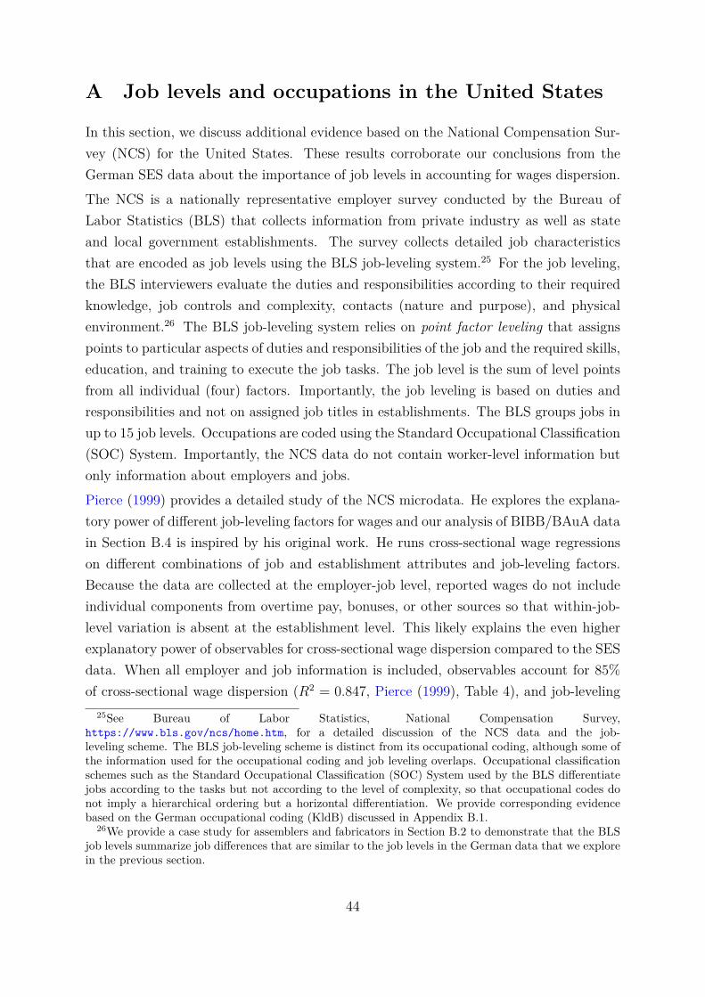
A Job levels and occupations in the United States

In this section, we discuss additional evidence based on the National Compensation Sur-vey (NCS) for the United States. These results corroborate our conclusions from theGerman SES data about the importance of job levels in accounting for wages dispersion.The NCS is a nationally representative employer survey conducted by the Bureau ofLabor Statistics (BLS) that collects information from private industry as well as stateand local government establishments. The survey collects detailed job characteristicsthat are encoded as job levels using the BLS job-leveling system.2525 For the job leveling,the BLS interviewers evaluate the duties and responsibilities according to their requiredknowledge, job controls and complexity, contacts (nature and purpose), and physicalenvironment.2626 The BLS job-leveling system relies on point factor leveling that assignspoints to particular aspects of duties and responsibilities of the job and the required skills,education, and training to execute the job tasks. The job level is the sum of level pointsfrom all individual (four) factors. Importantly, the job leveling is based on duties andresponsibilities and not on assigned job titles in establishments. The BLS groups jobs inup to 15 job levels. Occupations are coded using the Standard Occupational Classification(SOC) System. Importantly, the NCS data do not contain worker-level information butonly information about employers and jobs.PiercePierce (19991999) provides a detailed study of the NCS microdata. He explores the explana-tory power of different job-leveling factors for wages and our analysis of BIBB/BAuA datain Section B.4B.4 is inspired by his original work. He runs cross-sectional wage regressionson different combinations of job and establishment attributes and job-leveling factors.Because the data are collected at the employer-job level, reported wages do not includeindividual components from overtime pay, bonuses, or other sources so that within-job-level variation is absent at the establishment level. This likely explains the even higherexplanatory power of observables for cross-sectional wage dispersion compared to the SESdata. When all employer and job information is included, observables account for 85%of cross-sectional wage dispersion (R2 = 0.847, PiercePierce (19991999), Table 4), and job-leveling

25See Bureau of Labor Statistics, National Compensation Survey,https://www.bls.gov/ncs/home.htmhttps://www.bls.gov/ncs/home.htm, for a detailed discussion of the NCS data and the job-leveling scheme. The BLS job-leveling scheme is distinct from its occupational coding, although some ofthe information used for the occupational coding and job leveling overlaps. Occupational classificationschemes such as the Standard Occupational Classification (SOC) System used by the BLS differentiatejobs according to the tasks but not according to the level of complexity, so that occupational codes donot imply a hierarchical ordering but a horizontal differentiation. We provide corresponding evidencebased on the German occupational coding (KldB) discussed in Appendix B.1B.1.

26We provide a case study for assemblers and fabricators in Section B.2B.2 to demonstrate that the BLSjob levels summarize job differences that are similar to the job levels in the German data that we explorein the previous section.

44

Table 8: Mean wages in 2015 by job level and occupational group

Occupational groups (SOC)

Level 11-29 31-39 41-43 45-49 51-53 All

All 38.22 12.58 17.34 23.09 17.87 23.25

1 8.55 9.63 10.01 9.252 9.63 10.53 14.26 12.09 10.483 13.01 11.15 12.83 14.78 15.62 12.894 15.42 13.67 16.32 18.23 19.67 16.395 18.80 18.84 20.14 21.11 20.95 20.136 20.96 21.83 24.42 27.47 24.92 23.777 24.63 28.03 30.56 30.67 31.27 27.178 32.11 33.14 38.82 34.12 32.929 37.50 62.13 38.3210 42.68 44.5511 50.65 53.2612 69.37 73.13

Notes: Mean wages by job level and occupational groups from the 2015 National Compensation Survey.Occupational groups follow the 2010 SOC codes. The different occupational groups correspond roughly toManagement, Business and Finance, IT and Engineering, Education, Legal, Healthcare (11-29), Service(31-39), Sales and Administration (41-43), Farming, Construction, Maintenance (45-49), and Productionand Transportation (51-53). See SOC classification for further details. Missing fields indicate the caseof too few observations for a combination of job level and occupational group to be reported by theBLS. These estimates are currently not published by the BLS and have been provided by the BLS uponrequest.

factors alone account for 75% of wage variation. These results corroborate key findingsfrom our previous analysis of SES data. First, employer surveys with detailed job char-acteristics deliver high explanatory power on wage dispersion, and second, the job levelsare a key contributor to the high explanatory power of wage dispersion in these data. Asa first summary, we find that the high explanatory power of an additional dimension oftask execution accounts also in US data for a large part of wage dispersion, so that thisfinding is not a particularity of the German labor market and its institutions.Next, we explore the relationship between occupational wage differences and job-levelwage differences in the NCS data. The BLS provides information on average wages byjob level both across and within occupations. Table 88 shows mean wages by job leveland occupational group from the 2015 NCS.2727 We see that within coarse occupational

27These estimates are currently not published by the BLS and have been provided by the BLS uponan individual request for data.

45

groups, there is a wide variation of wages across job levels. For example, looking at alljobs, we see that going from job level 3 (paying on average $13) to job level 8 means awage increase of $20 per hour. Climbing further to job levels 10, 11, and 12 will lead tostellar wage increases of $30, $40, or $60 per hour. If anything, these data suggest thatclimbing the career ladder is more important in the United States than in Germany. Wealso note that when looking across occupation groups that the first occupation group (11-29), which includes management occupations, has on average much higher wages than theother groups. Strikingly, once we condition on the job level, the occupation group (11-29)tends to have below-average wages. For example, at job level 7 management occupationspay $24.63 , which is less than the average over all occupations at level 7; the latter being$27.17. Generally, we find that relative wage differences across occupation groups aresmall and (with one exception) less than 20% once we condition on job levels.

Figure 11: Occupation wage premia and within-occupation wage dispersion

−.5

0.5

1 without job−level controls

with job−level controls

(a) occupation wage premia

0.2

.4.6 without job−level controls

with job−level controls

(b) within-occupation wage dispersion

Notes: Left panel: estimated occupation wage premia after controlling for employer and job character-istics with and without job-leveling factors in the National Compensation Survey (NCS). See text fordetails. Right panel: residual within-occupation wage variance after controlling for employer and jobcharacteristics with and without job-leveling factors in the NCS. All estimation results are taken fromTable 7 in PiercePierce (19991999).

The fact that raw differences in occupational wages are largely driven by differences in theaverage job level of an occupation is also shown in PiercePierce (19991999). PiercePierce explores occupa-tional wage premia and within-occupation wage differences with and without controllingfor job-level factors. The results are striking. He finds that most of the occupational wagedifferences disappear once job-leveling factors have been taken into account and that evenwithin-occupation groups, on average 50% of the wage dispersion can be accounted forby job-leveling factors. These findings align closely with our findings that occupations donot account for a large part of wage growth. Figure 1111 visualizes results from Table 7 inPiercePierce (19991999). Figure 1111(a) shows occupational wage premia that are estimated as wage

46

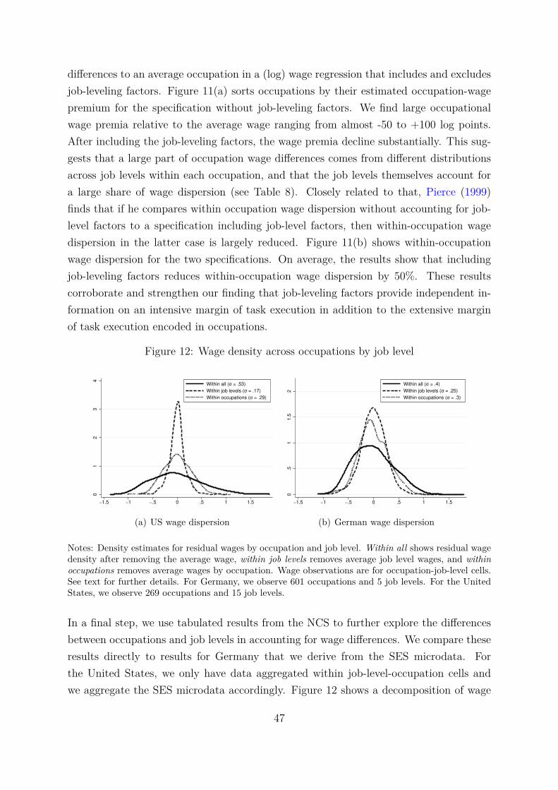
differences to an average occupation in a (log) wage regression that includes and excludesjob-leveling factors. Figure 1111(a) sorts occupations by their estimated occupation-wagepremium for the specification without job-leveling factors. We find large occupationalwage premia relative to the average wage ranging from almost -50 to +100 log points.After including the job-leveling factors, the wage premia decline substantially. This sug-gests that a large part of occupation wage differences comes from different distributionsacross job levels within each occupation, and that the job levels themselves account fora large share of wage dispersion (see Table 88). Closely related to that, PiercePierce (19991999)finds that if he compares within occupation wage dispersion without accounting for job-level factors to a specification including job-level factors, then within-occupation wagedispersion in the latter case is largely reduced. Figure 1111(b) shows within-occupationwage dispersion for the two specifications. On average, the results show that includingjob-leveling factors reduces within-occupation wage dispersion by 50%. These resultscorroborate and strengthen our finding that job-leveling factors provide independent in-formation on an intensive margin of task execution in addition to the extensive marginof task execution encoded in occupations.

Figure 12: Wage density across occupations by job level

01

23

4

−1.5 −1 −.5 0 .5 1 1.5

Within all (σ = .53)

Within job levels (σ = .17)

Within occupations (σ = .29)

(a) US wage dispersion

0.5

11.5

2

−1.5 −1 −.5 0 .5 1 1.5

Within all (σ = .4)

Within job levels (σ = .25)

Within occupations (σ = .3)

(b) German wage dispersion

Notes: Density estimates for residual wages by occupation and job level. Within all shows residual wagedensity after removing the average wage, within job levels removes average job level wages, and withinoccupations removes average wages by occupation. Wage observations are for occupation-job-level cells.See text for further details. For Germany, we observe 601 occupations and 5 job levels. For the UnitedStates, we observe 269 occupations and 15 job levels.

In a final step, we use tabulated results from the NCS to further explore the differencesbetween occupations and job levels in accounting for wage differences. We compare theseresults directly to results for Germany that we derive from the SES microdata. Forthe United States, we only have data aggregated within job-level-occupation cells andwe aggregate the SES microdata accordingly. Figure 1212 shows a decomposition of wage

47

differences across occupations and job levels for the 2010 NCS and the 2014 SES data.In both cases, we use average wages by occupation-job-level cell. For Germany, we focuson 2014 SES data because of the finer four-digit occupation codes (KldB classification)in these data: we observe 601 different occupations and 5 different job levels in the SESdata. These numbers imply that the number of occupations is 120 times larger than thenumber of observed job levels in the SES data. In the US NCS data, we observe 269occupations and 15 job levels. The ratio between occupations and job levels is still largewith 18 times more occupations than job levels. Figure 1212 shows density estimates forresidual (log) wages for three cases. In the first case, we remove average wages; that is,we show the variance of (log) wages. This is shown as the case within all. Second, weremove average wages by job level. This is shown as the case within job levels. Finally,we remove average wages by occupation. This is shown as the case within occupations.The legend also reports the estimated standard deviation for each case.2828 In the UScase, the 15 job levels account for roughly two-thirds of the cross-sectional standarddeviation, whereas 269 occupations account for only about a third of the cross-sectionalwage variation. For the German case, the findings are even more striking. The 5 joblevels account for about 40% of the cross-sectional variation, whereas 120 times as manyoccupation dummies (601 occupation codes) account for only about 25% of the cross-sectional wage variation.2929 In Appendix B.1B.1, we also report results for SES data resultsusing ISCO occupation codes and finer 5-digit occupation codes. For these occupationcodes, we observe 118 occupations for ISCO codes and 984 occupations for five-digitKldB occupation codes. Even for the finer five-digit occupation codes resulting in 984occupation dummies, we still find that we account for less of the cross-sectional wagedispersion across occupation-job-level cells than using only five job-level dummies.

B Details on job levels

In this section, we provide a detailed discussion on the distinction between job levelsand other job-related concepts and theories. In Section B.1B.1, we discuss the relationshipto occupations and modern occupational codes, specifically, the KldB2010 (Klassificationder Berufe 2010). Section B.3B.3 relates job levels to the task-based approach by Autor et al.Autor et al.(20032003) that classifies jobs by occupational tasks. Finally, Section B.4B.4 demonstrates thatjob levels can be constructed from job requirements and tasks and relates these resultsto the tournament theory of career progression (Lazear and RosenLazear and Rosen, 19811981).

28We use unweighted estimates across cells because the BLS does not release cell sizes for these data.29In the analysis before, we decompose the increase in wage dispersion over the life cycle, whereas here

we decompose the level of cross-sectional variation.

48

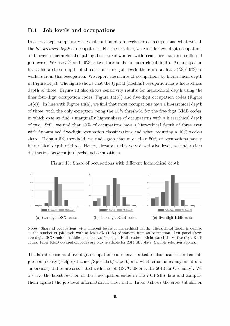
B.1 Job levels and occupations

In a first step, we quantify the distribution of job levels across occupations, what we callthe hierarchical depth of occupations. For the baseline, we consider two-digit occupationsand measure hierarchical depth by the share of workers within each occupation on differentjob levels. We use 5% and 10% as two thresholds for hierarchical depth. An occupationhas a hierarchical depth of three if on three job levels there are at least 5% (10%) ofworkers from this occupation. We report the shares of occupations by hierarchical depthin Figure 14(a)14(a). The figure shows that the typical (median) occupation has a hierarchicaldepth of three. Figure 1313 also shows sensitivity results for hierarchical depth using thefiner four-digit occupation codes (Figure 14(b)14(b)) and five-digit occupation codes (Figure14(c)14(c)). In line with Figure 14(a)14(a), we find that most occupations have a hierarchical depthof three, with the only exception being the 10% threshold for the five-digit KldB codes,in which case we find a marginally higher share of occupations with a hierarchical depthof two. Still, we find that 40% of occupations have a hierarchical depth of three evenwith fine-grained five-digit occupation classifications and when requiring a 10% workershare. Using a 5% threshold, we find again that more than 50% of occupations have ahierarchical depth of three. Hence, already at this very descriptive level, we find a cleardistinction between job levels and occupations.

Figure 13: Share of occupations with different hierarchical depth

0.2

.4.6

.8

1 2 3 4 5

5% threshold 10% threshold

(a) two-digit ISCO codes

0.2

.4.6

1 2 3 4 5

5% threshold 10% threshold

(b) four-digit KldB codes

0.1

.2.3

.4.5

1 2 3 4 5

5% threshold 10% threshold

(c) five-digit KldB codes

Notes: Share of occupations with different levels of hierarchical depth. Hierarchical depth is definedas the number of job levels with at least 5% (10%) of workers from an occupation. Left panel showstwo-digit ISCO codes. Middle panel shows four-digit KldB codes. Right panel shows five-digit KldBcodes. Finer KldB occupation codes are only available for 2014 SES data. Sample selection applies.

The latest revisions of five-digit occupation codes have started to also measure and encodejob complexity (Helper/Trained/Specialist/Expert) and whether some management andsupervisory duties are associated with the job (ISCO-08 or KldB-2010 for Germany). Weobserve the latest revision of these occupation codes in the 2014 SES data and comparethem against the job-level information in these data. Table 99 shows the cross-tabulation

49

of the last digits of the occupational classification system KldB 2010 of the Germanemployment agency against job-level information in the 2014 SES data. We find a clearpositive correlation between the information from the occupation code and the job level,but we also see that there is substantial mass off-diagonal.

Table 9: Cross-tabulation of job levels measured directly and job levels inferred fromoccupation codes

Complexitymeasured byoccupation

Fraction ofoccupation(in %)

Fraction of job levels within occupation (in %)

UT TR AS PR MA

All 100 6.4 13.4 50.1 19.9 10.4

from last digit (KldB 2010)Helper 13.4 29.6 40.4 27.4 2.0 0.6Trained 55.6 4.0 13.2 69.2 11.3 2.4Specialist 15.8 0.7 2.9 35.8 50.9 9.6Expert 15.2 0.5 1.1 14.7 34.7 48.9

using management occupations (KldB 2010)Supervisors 2.3 0.9 3.3 32.8 42.1 20.9Managers 2.9 0.6 1.3 15.9 30.5 51.6

Notes: Cross-tabulation of job levels and job information provided by the German Statistical Officebased on data from the 2014 Structure of Earnings Survey. Occupational information extracted fromfive-digit occupational code (KldB 2010). The first part of the table (last digit) shows the distributionof workers by occupational complexity across job-level groups. Shares sum to 100 within each row. Thefirst column (total) shows the population share of the occupation group. The second part of the table(management occupations) shows the distribution of occupations coded as supervisors or managers acrossjob-level groups. Shares sum to 100 within each row. The numbers in the columns refer to the share ofworkers coded as supervisors or managers in the total population.

In Appendix AA, we compare already estimated wage densities and standard deviationsacross occupation-job-level cells from US NCS data and German 2014 SES data. ForGerman data in Figure 1212, we use four-digit KldB occupation codes to define occupationcells. Figure 1414 shows sensitivity results using three-digit ISCO occupation codes and five-digit KldB codes. Differences between occupation and job-level densities are still largeand demonstrate that the larger explanatory power of job levels compared to occupationsis robust to using different levels of occupational disaggregation.Figure 1414(a) shows results for three-digit ISCO codes with 118 different occupations.We again find that five job-level dummies account for 40% of the wage dispersion acrossoccupation-job-level cells, while the 118 occupation dummies account for only about 15%of this wage dispersion. The difference becomes even more striking in the case of thefive-digit KldB codes in Figure 1414(b). The 984 occupation dummies account for less

50

Figure 14: Wage density across occupations by job level for different occupation codes0

.51

1.5

2

−1.5 −1 −.5 0 .5 1 1.5

Within all (σ = .38)

Within job levels (σ = .23)

Within occupations (σ = .32)

(a) three-digit ISCO codes

0.5

11.5

2

−1.5 −1 −.5 0 .5 1 1.5

Within all (σ = .4)

Within job levels (σ = .26)

Within occupations (σ = .27)

(b) five-digit KldB codes

Notes: Density estimates for residual wages by occupation and job level. Within all shows residualwage density after removing the average wage, within job levels removes average job-level wages, andwithin occupations removes average wages by occupation. Wage observations are for occupation-job-levelcells. The number of cells varies with the occupation codes applied. See text for further details. Forthree-digit ISCO codes, we observe 118 different occupations, and for five-digit KldB codes, we observe984 occupations. We always observe 5 job levels.

of the wage dispersion across occupation-job-level cells than five job-level dummies thataccount for 35% of the wage dispersion.

B.2 Case study of within-occupation job-level differences

To further substantiate the differences between occupations and job levels and to high-light that these differences also apply beyond the German case, we consider a case studyfor a narrowly defined occupation group: assemblers and fabricators in production. Forour case study, we start with the German union bargaining agreement for metal- andsteelworkers in North-Rhine-Westphalia. This union bargaining agreement has at itscore an analytic job-leveling scheme to assign workers to wage scales; it is closely com-parable to the BLS job-leveling scheme and which we use for our analysis in SectionB.4B.4. Together with the job level, we also observe the bargained wage for each job level.3030

For assemblers (Montierer) and fabricators (Maschinen- und Anlagenbauer), we havejob-leveling information that distinguishes these occupations at six different job levels:four job levels for the occupation group assemblers and two for fabricators.3131 We usethe German job-leveling information (i.e., specific job descriptions regarding tasks and

30These bargained wages are lower bounds for wages and are typically supplemented by performancecomponents that are worker- and firm-specific.

31One occupation has no directly assigned occupation title but comes from the same task section(Aufgabenfamilie).

51

duties of the jobholder) to assign job levels based on the BLS job-leveling guide. Usingthe resulting job levels, we assign wages for full-time workers from the tabulations forproduction occupations from the NCS in 2010.3232 In the NCS data, we stay within a singleoccupation group according to the classification in the 2000 SOC System and use onlywages at different job levels. After leveling the German jobs using the BLS procedure,we remove mean wage differences between Germany and the United States so that theaverage across the assigned wages is one in both countries.

Figure 15: Leveling wage structures for assemblers and fabricators in production

0.5

11

.5

1 2 3 5 9 11

Germany United States

Notes: Standardized wages for assemblers and fabricators in production for the United States and Ger-many. German wages are taken from the union bargaining agreement for metal- and steelworkers inNorth-Rhine Westphalia. Wages for the United States are derived using the BLS job-leveling approachand NCS wage information by occupation and job level. The job levels are taken from the metal- andsteelworkers’ bargaining agreement. See text for details.

Figure 1515 shows the standardized wage differences across job levels for Germany and theUnited States. We find that wage structures show a similar shape across countries, withthe key difference being that the German wage structure shows more wage compressionespecially in the lower part. This type of wage compression is typically associated withunion wage bargaining in Germany. Overall, we find wages to be roughly flat across thefirst four groups in Germany and the first three groups in the United States, and find apositive gradient across the upper three groups. Hence, qualitatively the estimates forthe corresponding US jobs show a very similar pattern but show more wage dispersionoverall. Part of the differences might be because job-level wages in the German collectivebargaining agreement only include base pay, whereas they also include incentive and

32United States Department of Labor, Bureau of Labor Statistics, National Compensation Survey —Wages, Table 8: Civilian workers: Mean hourly earnings for full-time and part-time workers by worklevels, https://www.bls.gov/ncs/ocs/sp/nctb1482.txthttps://www.bls.gov/ncs/ocs/sp/nctb1482.txt.

52

performance pay in the data for the United States. In addition, the wages for Germany areonly wages under the specific union bargaining agreement in one state that likely featureswage compression. Despite these caveats, we take this case study of a narrowly definedoccupational group as further evidence for the importance of job levels and intensivemargin variation in task execution for determining wages and wage differences in Germanyand the United States.

B.3 Job levels and task-based classification of jobs

Job levels as a common component in occupational wage premia parallels the idea fromthe influential task-based approach by Autor et al.Autor et al. (20032003) that classifies jobs along thedimensions cognitive vs. manual tasks and routine vs. non-routine tasks. The task-basedapproach formalizes the idea that some tasks can be executed by computers because taskexecution follows a fixed set of routines (routine tasks,) while others are not amenableto being put into a computer program (non-routine tasks). In fact, categorizing jobs interms of responsibility, autonomy, and complexity has the flavor of ranking jobs alongtheir cognitive-non-routine intensity dimension.There are two key differences of the task-based approach to job leveling. First, thetask-based approach is derived from occupation-level information (not as the Cartesianproduct of occupations and job levels) so that it does not differentiate within occupations,while job levels provide within-occupation differentiation (Appendices B.1B.1 and B.2B.2). Sec-ond, one way to interpret the task-based approach is that it projects occupational taskson their amenability to being executed by a computer.3333 This projection aligns mostclosely with the autonomy that is part of the job level but it does not relate directly toresponsibility and complexity. Even for autonomy, there would be no distinction betweenthe baker who decides about the amount of the ingredients and the baking time and thebaker who mixes the ingredients together.It seems natural to wonder whether five-digit occupation codes contain all the job-levelinformation and whether they are already fine grained enough so that there is no ad-ditional information in job levels. Appendix B.1B.1 answers this question in detail andprovides a strong negative answer. Even at the five-digit level, most occupations span atleast two job levels, and many still have a substantial share of workers on three job levels(out of five). Appendix B.2B.2 provides additional evidence based on a case study wherewe construct job levels within a single occupation. But even if most occupations spanmany job levels, not all occupations are alike in terms of their average job level. Workers

33Examples of tasks from Appendix Table 1 in Autor et al.Autor et al. (20032003) are “computes discount, interest,profit, and loss,” “mixes and bakes ingredients according to recipes.”

53

in some occupations have on average higher job levels than other occupations (Table 88).This variation in average job level allows us to shed some more light on the relationshipof job levels and the cognitive/non-routine classification of occupations.

B.3.1 Correlation between job levels and occupational tasks

In their description of jobs, Autor et al.Autor et al. (20032003) emphasize the amenability of tasks to beautomated using computer software. They distinguish between routine tasks that canbe done by computers and non-routine tasks that cannot be executed by computer pro-grams. They classify occupations based on the description of the occupational tasks usingthis task-based approach. In addition to routine and non-routine tasks, they distinguishmanual and cognitive, analytic and interactive tasks. Their task-based classification ofoccupations consists of five groups: non-routine analytic, non-routine interactive, routinecognitive, routine manual, and non-routine manual. Using the task-based approach theyexplore how the proliferation of computers due to a decline in prices affected employmenttrends between 1960 and 1998. The task-based approach has also been implementedfor the German labor market by Spitz-OenerSpitz-Oener (20062006) and Dengler et al.Dengler et al. (20142014). For thetask-based classification, Dengler et al.Dengler et al. (20142014) follow closely the original approach byAutor et al.Autor et al. (20032003) by relying on expert assessments of job task contents. Spitz-OenerSpitz-Oener(20062006) classifies occupations based on BIBB/BAuA survey data on workers to assign tasksto occupations. We use the classification by Dengler et al.Dengler et al. (20142014) based on 2013 occupa-tional tasks to the 2014 SES data aggregated to the three-digit occupation level. Beforeaggregating the SES microdata, we apply the sample selection as described in Section33. Our final occupation sample has information on 137 occupations (3-digit KldB2010),their mean log wages and mean job levels from the SES data and the task contents fornon-routine analytic (A-NR), non-routine interactive (I-NR), routine cognitive (C-R),routine manual (M-R), and non-routine manual (M-NR) tasks and the main task cate-gory from Dengler et al.Dengler et al. (20142014). Task contents are measured as task shares summing to100% with each occupation.In Table 1010, we look at correlations between the average occupation job level and taskshares. The key idea of the task-based approach in Autor et al.Autor et al. (20032003) is that routinetasks can be replaced by computers and that non-routine tasks are relative complementsto computer capital. In line with the fact that autonomy is one of the key components ofjob levels and at the same time captures how much workers have to follow a fixed set ofrules and cannot make individual decision on the work flow, we find that the non-routineanalytic and cognitive task shares correlate positively with the average job level. Fornon-routine manual, we find a negative correlation pointing to the fact that job levels

54

also capture the complexity and skill requirements of a job that are typically low formanual jobs.

Table 10: Task components and average job levels

A-NR I-NR C-R M-R M-NR

job level 0.68 0.22 0.14 -0.48 -0.47

Notes: Correlation coefficients between average job level and occupation task shares for non-routine an-alytic (A-NR), non-routine interactive (I-NR), routine cognitive (C-R), routine manual (M-R), and non-routine manual (M-NR). Data for 137 occupations (3-digit KldB2010) from 2014 SES and Dengler et al.Dengler et al.(20142014).

To explore these correlations in more detail, Figure 1616 shows scatter plots of the averagejob level and the shares of the different task components. Looking at Figure 1616(a), wefind the clearly upward-sloping relationship between job levels and the share of analyticnon-routine tasks. Yet, there is also substantial dispersion. For the interactive non-routine component in Figure 1616(b), the data are much more dispersed and a positiverelationship is less striking. The cognitive routine tasks in Figure 1616(c) show a positiverelationship, yet again, there is also substantial dispersion. For the manual routine tasksin Figure 1616(d), we observe that occupations with average job levels of 3 and higherhardly comprise any manual routine tasks. There is a strong decline in the share for jobswith average job levels between 2 and 3. The pattern for the manual non-routine tasks inFigure 1616(e) largely resembles the pattern for the manual routine tasks. This similaritylikely highlights that within manual routine occupations there are also foremen and groupleader who have to act autonomously in the production process and have responsibilityfor the work of their group members. As the task-based classification is coded fromdescriptions of occupations and their typical tasks, by construction, it does not allow forwithin-occupation differences in task content. For example, an architect who “plans anddesigns private residences, office buildings, factories, and other structures” is carrying-outnon-routine interactive tasks as can be seen in Appendix 1 table of Autor et al.Autor et al. (20032003).Yet, there are likely differences in job levels across architects. While the architect atthe (MA)nagement job level decides how the building is going to look, an architect atthe specialist level has to work out the planning details according to the plan of thearchitect at the management level. Job levels capture this additional distinction withinoccupational task execution that we label as the intensity of task execution. Figure 1616(f)uses information on the main task of an occupation, the task category with the largesttask share, and compares it to the average job level. We find that occupations thatheavily load on analytic non-routine tasks have on average higher job levels, while manual

55

routine occupations have the lowest average job levels. This correlation between tasksand job levels is already apparent in Table 88, where we find for the United States thatmanagement occupations populate higher job levels than service occupations but that,conditional on the job levels, wages do not differ notably. For all main task categories,we observe substantial dispersion of average job levels.

Figure 16: Tasks and job levels

0.2

.4.6

.81

av.

A−

NR

sh

are

1 2 3 4 5av. job level

(a) A-NR

0.2

.4.6

av.

I−N

R s

ha

re

1 2 3 4 5av. job level

(b) I-NR

0.2

.4.6

.8a

v.

C−

R s

ha

re

1 2 3 4 5av. job level

(c) C-R

0.2

.4.6

.8a

v.

M−

R s

ha

re

1 2 3 4 5av. job level

(d) M-R

0.2

.4.6

.81

av.

M−

NR

sh

are

1 2 3 4 5av. job level

(e) M-NR

12

34

5a

v.

job

le

ve

l

A−NR I−NR C−R M−R M−NR

(f) main task

Notes: Panels (a) to (e) show average occupation job levels against the five components constructedby the task-based approach: non-routine analytic (A-NR), non-routine interactive (I-NR), routine cog-nitive (C-R), routine manual (M-R), and non-routine manual (M-NR). Each dot represents one 3-digitKldB2010 occupation. Data are aggregated for 137 occupations from 2014 SES data and data providedby Dengler et al.Dengler et al. (20142014). Panel (f) shows a box plot of the average job level by main task of an occupa-tion. The main task is the task-based category with the largest task share as defined by Dengler et al.Dengler et al.(20142014).

B.3.2 Wages, job levels, and occupational tasks

Given the observed correlation between occupational task contents and job levels fromFigure 1616, we next ask how much each component contributes to occupational wagedifferences. We run a simple linear regression at the occupation level of log wages onaverage job levels and task contents of occupations

wi = α + βxi +∑c

γczi,c + εi

56

Table 11: Wages, tasks, and job levels

(1) (2) (3) (4) (5) (6) (7) (8)only JL JL + TBA only TBA A-NR I-NR M-R M-NR C-R

job level 0.48∗∗∗ 0.50∗∗∗(0.00) (0.00)

A-NR -0.14 0.33∗ 0.73∗∗∗(0.14) (0.02) (0.00)

I-NR -0.20∗ -0.28 0.21(0.05) (0.09) (0.21)

M-R 0.08 -0.28∗ -0.39∗∗∗(0.35) (0.05) (0.00)

M-NR -0.22∗∗ -0.52∗∗∗ -0.64∗∗∗(0.01) (0.00) (0.00)

C-R 0.34∗(0.02)

N 137 137 137 137 137 137 137 137adj. R2 0.743 0.774 0.377 0.309 0.005 0.073 0.256 0.035

Notes: Regression coefficients from regressing mean occupation log wages on average job levels andtask-based components. Wage and job level data are aggregated for 137 occupations from 2014 SESdata and task-based components are taken from Dengler et al.Dengler et al. (20142014). For each specification, number ofobservations and adjusted R2 are shown at the bottom of the table, p-values in parentheses, and *, **,*** indicate significance of coefficients at the 5%, 1%, and 0.1% levels, respectively. See text for furtherdetails.

where wi is the average log wage in occupation i, xi is the average job level of occupationi and zi,c are the task shares of occupation i. As task shares sum to 1, i.e.,

∑5c=1 zi,c = 1,

we drop the cognitive routine share if necessary to avoid collinearity. Table 1111 showsregression results for different specifications of the regression above.The first striking observation is the high explanatory power of the average job level forinter-occupational wage differences in the first specification (column (1) only JL) wherewe only regress on the average job level of an occupation. The next striking observationis that adding information from the task-based approach (column (2)) adds little to theexplanatory power of the regression and only the coefficients on interactive non-routine(I-NR) and manual non-routine (M-NR) tasks are statistically significant. If we onlyconsider the task-based approach in column (3), the explanatory power is only abouthalf that of the job levels alone. Most notably, analytic non-routine (A-NR) tasks have asignificant and strongly positive effect on inter-occupational wages. Manual non-routinetasks have a large negative effect on wages that is highly statistically significant. Whenwe run the different task components in isolation, we find that analytic non-routineand manual non-routine have the highest explanatory power for inter-occupational wage

57

differences but that the effect of analytic non-routine tasks on wages disappears and thecoefficient of manual non-routine tasks is cut by a factor of three once we control forthe average job level. Note furthermore that the point estimate for the average job levelremains virtually unaffected when we include the information from task-based approach(columns (1) and (2)). These results corroborate our findings of the large explanatorypower of job levels on between-occupation wage differences.

B.4 Job leveling and tournament models

One important concern regarding job levels is that they are simply a recoding of wages(e.g., wage quintiles) and for that reason “explain” wages well in a statistical sense, aform of reverse causality. The specific concern might be that, when asked to level the jobof a specific, say, well-paid, worker, an employer will assign a high job level without thatjob level actually reflecting the tasks and duties in this job. Instead, the employer justassigned the worker to the job because of her skills or past performance.To address this concern, we use additional data from the BIBB/BAuA EmploymentSurvey 2012 on job requirements, working conditions, and wages (Hall et al.Hall et al., 20182018) tovalidate our findings from the previous section outside the SES data. The SES data donot contain detailed information on tasks beyond what is contained in the job levels andoccupations, while the BIBB/BAuA data do.This analysis also addresses a key identification challenge for our analysis in Section 44that arises from economic theory. The tournament model by Lazear and RosenLazear and Rosen (19811981)is one of the seminal theories on career progression. In this theory, promotions are theoutcome of a tournament to incentivize workers’ provision of effort. In this case, thecurrent job and its tasks and duties do not determine a worker’s pay, but the worker isassigned to a job based on her past performance. If we find a high explanatory powerof current job characteristics for current wages of workers independent of information onthe worker performing the job, we also address this identification challenge by providingevidence supporting a fundamental role of task execution in determining wages.

B.4.1 Job contents and job-leveling factors

The BIBB/BAuA data provide information on wages, jobs and their characteristics inaddition to worker demographics and typical labor market data such as occupation, in-dustry, and employer size. We restrict the BIBB/BAuA sample to be in line with ourSES analysis. We keep workers ages 25 to 55 who work at employers with at least 10employees and drop workers in public service. We drop self-employed workers, freelance

58

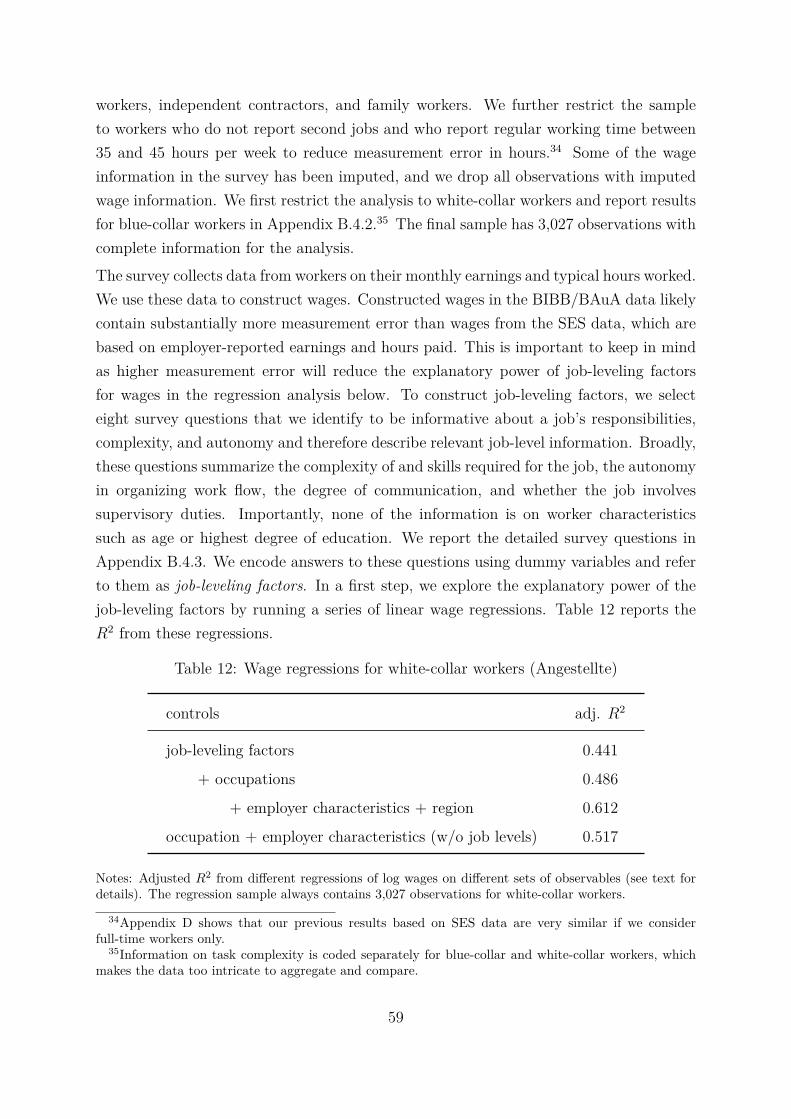
workers, independent contractors, and family workers. We further restrict the sampleto workers who do not report second jobs and who report regular working time between35 and 45 hours per week to reduce measurement error in hours.3434 Some of the wageinformation in the survey has been imputed, and we drop all observations with imputedwage information. We first restrict the analysis to white-collar workers and report resultsfor blue-collar workers in Appendix B.4.2B.4.2.3535 The final sample has 3,027 observations withcomplete information for the analysis.The survey collects data from workers on their monthly earnings and typical hours worked.We use these data to construct wages. Constructed wages in the BIBB/BAuA data likelycontain substantially more measurement error than wages from the SES data, which arebased on employer-reported earnings and hours paid. This is important to keep in mindas higher measurement error will reduce the explanatory power of job-leveling factorsfor wages in the regression analysis below. To construct job-leveling factors, we selecteight survey questions that we identify to be informative about a job’s responsibilities,complexity, and autonomy and therefore describe relevant job-level information. Broadly,these questions summarize the complexity of and skills required for the job, the autonomyin organizing work flow, the degree of communication, and whether the job involvessupervisory duties. Importantly, none of the information is on worker characteristicssuch as age or highest degree of education. We report the detailed survey questions inAppendix B.4.3B.4.3. We encode answers to these questions using dummy variables and referto them as job-leveling factors. In a first step, we explore the explanatory power of thejob-leveling factors by running a series of linear wage regressions. Table 1212 reports theR2 from these regressions.

Table 12: Wage regressions for white-collar workers (Angestellte)

controls adj. R2

job-leveling factors 0.441

+ occupations 0.486

+ employer characteristics + region 0.612

occupation + employer characteristics (w/o job levels) 0.517

Notes: Adjusted R2 from different regressions of log wages on different sets of observables (see text fordetails). The regression sample always contains 3,027 observations for white-collar workers.

34Appendix DD shows that our previous results based on SES data are very similar if we considerfull-time workers only.

35Information on task complexity is coded separately for blue-collar and white-collar workers, whichmakes the data too intricate to aggregate and compare.

59

When we run a regression on the job-leveling factors only, we account for 44% of wagevariation.3636 This high explanatory power aligns closely with our results for the SES data.In the SES data, job levels alone account for 46% of the overall wage variation. Addingoccupation information to the job-leveling factors increases the explanatory power onlyslightly to 49%. Such a small contribution also aligns with our results from the SES datawhere occupations account for only a very small fraction of the job component. If wefurther add employer characteristics, we account for 61% of the wage variation. In theSES data, a regression on plant characteristics and job levels accounts for 62% of thewage variation.In a second step, we construct job levels based on a job-leveling scheme. We applysuch a job-leveling scheme based on the answers to the eight survey questions underlyingour job-leveling factors. It is important to point out that the BIBB/BAuA survey wasnever designed to be used in combination with such a job-leveling scheme, so we haveto assign point values to questions and answers to these questions. As a job-levelingscheme, we rely on the leveling scheme underlying the German steel- and metalworkerbargaining agreement (ERA-Punktebewertungsbogen zur Bewertung von Arbeitsaufgaben),which is typically seen as the reference bargaining agreement in Germany. The fact thatthe survey contains questions that can be mapped onto the components from such anexisting job-leveling scheme provides suggestive evidence that these job characteristicsare considered relevant in practice. We describe our mapping of survey answers to thejob-leveling scheme in Appendix B.4.3B.4.3. After assigning each worker observation job-levelpoints depending on the answers to the survey question, we run a simple linear regressionof the log wage on the assigned total of job-level points, and this regression accounts for39% of the wage variation. This is slightly lower than the 44% from the more flexibleregression on job-leveling factors in Table 1212. Figure 1717 shows the relationship betweenjob-level points and the average log wage for each point level. Although there is stillsubstantial dispersion that in part reflects sampling uncertainty, the data show a clearpositive relationship between job-level points and average (log) wages. In Figure 1919, wereport the distribution of wages by point levels and show that for each point level, thedispersion is small.Three points are important to emphasize regarding these results. First, the coding ofjob-level points involves only eight survey questions regarding a job’s responsibility, com-plexity, and autonomy. Second, neither worker nor wage information has been used forassigning points to jobs. Third, the assignment of job-level points is very rough andrepresents our attempt to map answers to job-level points. Sophisticated data analysiscould likely considerably improve the in-sample fit between job-level points and wage

36The regression involves 18 dummies for answers to the eight questions and a constant.

60

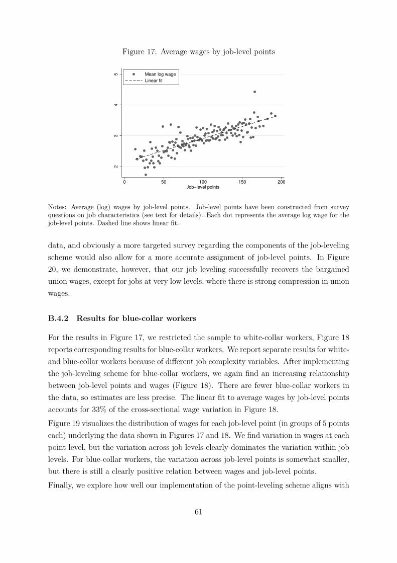
Figure 17: Average wages by job-level points

23

45

0 50 100 150 200Job−level points

Mean log wage

Linear fit

Notes: Average (log) wages by job-level points. Job-level points have been constructed from surveyquestions on job characteristics (see text for details). Each dot represents the average log wage for thejob-level points. Dashed line shows linear fit.

data, and obviously a more targeted survey regarding the components of the job-levelingscheme would also allow for a more accurate assignment of job-level points. In Figure2020, we demonstrate, however, that our job leveling successfully recovers the bargainedunion wages, except for jobs at very low levels, where there is strong compression in unionwages.

B.4.2 Results for blue-collar workers

For the results in Figure 1717, we restricted the sample to white-collar workers, Figure 1818reports corresponding results for blue-collar workers. We report separate results for white-and blue-collar workers because of different job complexity variables. After implementingthe job-leveling scheme for blue-collar workers, we again find an increasing relationshipbetween job-level points and wages (Figure 1818). There are fewer blue-collar workers inthe data, so estimates are less precise. The linear fit to average wages by job-level pointsaccounts for 33% of the cross-sectional wage variation in Figure 1818.Figure 1919 visualizes the distribution of wages for each job-level point (in groups of 5 pointseach) underlying the data shown in Figures 1717 and 1818. We find variation in wages at eachpoint level, but the variation across job levels clearly dominates the variation within joblevels. For blue-collar workers, the variation across job-level points is somewhat smaller,but there is still a clearly positive relation between wages and job-level points.Finally, we explore how well our implementation of the point-leveling scheme aligns with

61

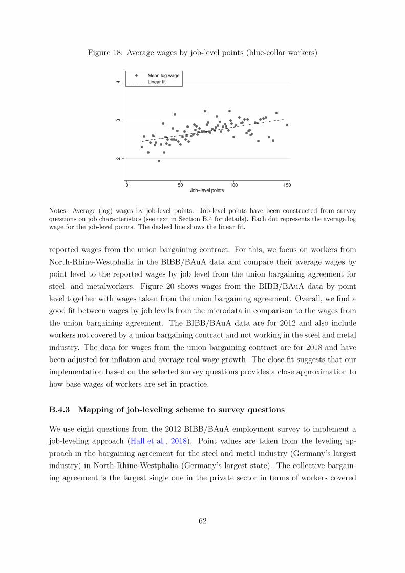
Figure 18: Average wages by job-level points (blue-collar workers)

23

4

0 50 100 150Job−level points

Mean log wage

Linear fit

Notes: Average (log) wages by job-level points. Job-level points have been constructed from surveyquestions on job characteristics (see text in Section B.4B.4 for details). Each dot represents the average logwage for the job-level points. The dashed line shows the linear fit.

reported wages from the union bargaining contract. For this, we focus on workers fromNorth-Rhine-Westphalia in the BIBB/BAuA data and compare their average wages bypoint level to the reported wages by job level from the union bargaining agreement forsteel- and metalworkers. Figure 2020 shows wages from the BIBB/BAuA data by pointlevel together with wages taken from the union bargaining agreement. Overall, we find agood fit between wages by job levels from the microdata in comparison to the wages fromthe union bargaining agreement. The BIBB/BAuA data are for 2012 and also includeworkers not covered by a union bargaining contract and not working in the steel and metalindustry. The data for wages from the union bargaining contract are for 2018 and havebeen adjusted for inflation and average real wage growth. The close fit suggests that ourimplementation based on the selected survey questions provides a close approximation tohow base wages of workers are set in practice.

B.4.3 Mapping of job-leveling scheme to survey questions

We use eight questions from the 2012 BIBB/BAuA employment survey to implement ajob-leveling approach (Hall et al.Hall et al., 20182018). Point values are taken from the leveling ap-proach in the bargaining agreement for the steel and metal industry (Germany’s largestindustry) in North-Rhine-Westphalia (Germany’s largest state). The collective bargain-ing agreement is the largest single one in the private sector in terms of workers covered

62

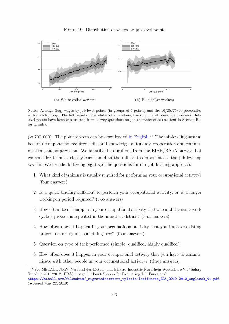
Figure 19: Distribution of wages by job-level points2

34

5

0 50 100 150 200Job−level points

Mean

p25−p75

p10−p90

(a) White-collar workers

23

4

0 50 100 150Job−level points

Mean

p25−p75

p10−p90

(b) Blue-collar workers

Notes: Average (log) wages by job-level points (in groups of 5 points) and the 10/25/75/90 percentileswithin each group. The left panel shows white-collar workers, the right panel blue-collar workers. Job-level points have been constructed from survey questions on job characteristics (see text in Section B.4B.4for details).

(≈ 700, 000). The point system can be downloaded in Englishin English.3737 The job-leveling systemhas four components: required skills and knowledge, autonomy, cooperation and commu-nication, and supervision. We identify the questions from the BIBB/BAuA survey thatwe consider to most closely correspond to the different components of the job-levelingsystem. We use the following eight specific questions for our job-leveling approach:

1. What kind of training is usually required for performing your occupational activity?(four answers)

2. Is a quick briefing sufficient to perform your occupational activity, or is a longerworking-in period required? (two answers)

3. How often does it happen in your occupational activity that one and the same workcycle / process is repeated in the minutest details? (four answers)

4. How often does it happen in your occupational activity that you improve existingprocedures or try out something new? (four answers)

5. Question on type of task performed (simple, qualified, highly qualified)

6. How often does it happen in your occupational activity that you have to commu-nicate with other people in your occupational activity? (three answers)

37See METALL NRW: Verband der Metall- und Elektro-Industrie Nordrhein-Westfalen e.V., “SalarySchedule 2010/2012 (ERA),” page 6, “Point System for Evaluating Job Functions”https://metall.nrw/fileadmin/_migrated/content_uploads/Tarifkarte_ERA_2010-2012_englisch_01.pdfhttps://metall.nrw/fileadmin/_migrated/content_uploads/Tarifkarte_ERA_2010-2012_englisch_01.pdf(accessed May 22, 2019).

63

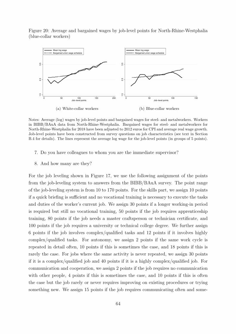
Figure 20: Average and bargained wages by job-level points for North-Rhine-Westphalia(blue-collar workers)

1.5

2.5

3.5

0 50 100 150 200Job−level points

Mean log wage

Bargained union wage schedule

(a) White-collar workers

1.5

2.5

3.5

0 50 100 150Job−level points

Mean log wage

Bargained union wage schedule

(b) Blue-collar workers

Notes: Average (log) wages by job-level points and bargained wages for steel- and metalworkers. Workersin BIBB/BAuA data from North-Rhine-Westphalia. Bargained wages for steel- and metalworkers forNorth-Rhine-Westphalia for 2018 have been adjusted to 2012 euros for CPI and average real wage growth.Job-level points have been constructed from survey questions on job characteristics (see text in SectionB.4B.4 for details). The lines represent the average log wage for the job-level points (in groups of 5 points).

7. Do you have colleagues to whom you are the immediate supervisor?

8. And how many are they?

For the job leveling shown in Figure 1717, we use the following assignment of the pointsfrom the job-leveling system to answers from the BIBB/BAuA survey. The point rangeof the job-leveling system is from 10 to 170 points. For the skills part, we assign 10 pointsif a quick briefing is sufficient and no vocational training is necessary to execute the tasksand duties of the worker’s current job. We assign 30 points if a longer working-in periodis required but still no vocational training, 50 points if the job requires apprenticeshiptraining, 80 points if the job needs a master craftsperson or technician certificate, and100 points if the job requires a university or technical college degree. We further assign6 points if the job involves complex/qualified tasks and 12 points if it involves highlycomplex/qualified tasks. For autonomy, we assign 2 points if the same work cycle isrepeated in detail often, 10 points if this is sometimes the case, and 18 points if this israrely the case. For jobs where the same activity is never repeated, we assign 30 pointsif it is a complex/qualified job and 40 points if it is a highly complex/qualified job. Forcommunication and cooperation, we assign 2 points if the job requires no communicationwith other people, 4 points if this is sometimes the case, and 10 points if this is oftenthe case but the job rarely or never requires improving on existing procedures or tryingsomething new. We assign 15 points if the job requires communicating often and some-

64

times requires improving on existing procedures, and we assign 20 points if it is oftenthe case that the job requires improving on existing procedures or trying something new.Finally for responsibility, we assign 10 points if the job includes supervisory duties and10 additional points if the job involves supervising more than 20 other workers. We sumthese job-level points to the total job-level points for each observation in the data.

C Instrumental variable regression

This section reports the estimation results for our instrumental variable approach. Theinstrumental variable approach addresses the concern that differences in the organiza-tional structure and job composition across cohorts that we use for identification in ourbaseline approach in Section 44 could be endogenous to the composition of workers in thesecohorts. To address this potential endogeneity problem, we instrument job levels usinga Bartik-type instrument (BartikBartik, 19931993). To construct our instrument for the job-levelcomponent, we only exploit changes in the industry composition over time and constructbased on the average job composition of an industry over the entire sample period, thepredicted occupation and job-level composition for each cohort at each moment in time.We then estimate the synthetic cohort approach by applying these instruments. We pro-ceed with the decomposition of wage growth and wage dispersion over the life cycle as inthe baseline case. Figure 2121 shows the resulting decomposition results for wage growthand wage inequality for males (Figures 2121(a) and 2121(c)) and for females (Figures 2121(b)and 2121(d)).In the decomposition of wage growth, we find that for both males (Figure 2121(a)) andfemales (Figure 2121(b)), the relative importance of the job component increases slightly,while the individual component decreases in its relative importance. In the decompositionof the increase in wage inequality, the results become even more striking than in ourbaseline approach. We find that for both males (Figure 2121(c)) and females (Figure 2121(d)),the relative importance of the job component increases and does track the overall increasealmost one-for-one. These results demonstrate that the results of our baseline approachfor the job component are robust to the potential endogeneity problem of labor supplyon the organizational structure and job composition of plants.

65

Figure 21: Decomposition of wage growth and wage dispersion over the life cycle usingIV approach

0.1

.2.3

.4.5

25 30 35 40 45 50 55

Total Individual component

Plant component Job component

(a) Growth (males)

0.0

5.1

.15

.2.2

5

25 30 35 40 45 50 55

Total Individual component

Plant component Job component

(b) Growth (females)

0.0

5.1

.15

.2.2

5

25 30 35 40 45 50 55

Total Individual component

Plant component Job component

(c) Variance (males)

0.0

5.1

.15

.2

25 30 35 40 45 50 55

Total Individual component

Plant component Job component

(d) Variance (females)

Notes: Contribution of the job component to wage growth (top row) and wage dispersion (bottomrow) for males (left panels) and females (right panels). The solid line shows the job component forthe baseline from the main part of the paper; the short dashed line shows the case with no collectivebargaining interaction; the dotted line shows the case with full-time interaction; and the dash-dottedline shows the case with large firm interaction. Job components have been constructed by setting alldummy variables in the interaction terms to one. As in the main text, all graphs show the coefficientsof age dummies of a regression of the components on a full set of age and cohort dummies (ages definedas three-year groups).

66

D Sensitivity analysis, extensions, and further re-sults

We provide several sensitivity checks to our baseline analysis from the main part ofthe paper. In the sensitivity checks, we explore the effects of not being covered by acollective bargaining agreement, considering only full-time work, or focusing on largeestablishments. We also show the results if we do not drop public employers from thesample or do not control for individual fixed effects using the synthetic panel regression.We discuss these results in Section D.1D.1. Sections D.2D.2, D.3D.3, and D.4D.4 explore more flexiblespecifications for the wage equation. Section D.5D.5 reports results if instead of a syntheticpanel approach, we rely on a pooled OLS regression when decomposing wages. Section D.6D.6reports the life-cycle profiles of residual wage dispersion from our decomposition. Finally,Section D.7D.7 reports the corresponding results for females of the wage decompositionwithout a job component (see Section 5.35.3 for males).

D.1 Heterogeneous returns to job and individual characteristics

For the first set of sensitivity checks, we interact variables from the baseline regressionin equation (33) with dummy variables for not being covered by a collective bargainingagreement, for working full-time, and for working in a large establishment. In Table 1313,we compare the baseline sample to the part of the sample that gets a positive dummyin the sensitivity analysis. Overall, there are differences in the job-level compositionin the alternative groups compared to the baseline sample, but they are not striking.We also report results for a sensitivity analysis in which we do not drop observationsfrom public employers and publicly controlled firms. The last column of Table 1313 showscharacteristics of workers and jobs at public employers that we drop for the baselineanalysis. Two observations are noteworthy for this sample of public employers. First, theshare of females is large: almost two-thirds of employees at public employers are female.Second, the job composition at public employers has fewer jobs at the untrained, trained,and assistant job levels but more jobs at the professional and management job levels.In the first step, we consider the sensitivity analysis with respect to collective bargainingagreements, full-time workers, and large establishments and test whether the estimatedcoefficients on the additional interaction terms are statistically significant. Table 1414shows test statistics for three tests for the three different interaction specifications. Thefirst row jointly tests all interaction coefficients. We find that insignificance can alwaysbe strongly rejected. When we look more closely at the different components, we findthat the coefficients on the interaction terms with the variables of the job component

67

Table 13: Summary Statistics

baseline no collective only large plants publicbargaining full-time employers

wage 18.9 17.8 19.9 22.0 19.4age 41.1 40.6 40.8 41.3 42.1female 38.9 37.9 27.2 37.3 61.9

UT 8.6 7.4 6.5 8.1 4.9TR 16.4 19.0 15.3 14.3 7.0AS 45.2 49.0 44.9 40.7 37.3PR 21.5 17.3 23.5 25.6 29.3MA 8.4 7.2 9.8 11.3 21.4

N (million) 2.4 1.3 1.9 0.9 1.4

Notes: Descriptive statistics of sample composition for baseline sample and subsamples considered insensitivity analysis. The rows wage and age refer to the sample averages. The row female refers to theshare of females in the sample; UT, TR, AS, PR, and MA show the shares for workers at the differentjob levels in the samples; and N is the number of observations in millions of the different samples.

(third row) are always strongly significant. The coefficients on the interactions with theindividual component are insignificant in the no collective bargaining case and significantin the two other cases (second row). The main part of the paper finds that job levels arethe key variable of the job component to account for both wage growth and dispersionover the life cycle. When we look at the coefficients of the interaction terms with thejob-level dummies, we find them to be always strongly statistically significant except forlarge plants where they are significant at the 10% level (fourth row).This finding means that potentially there is a layer of heterogeneity that is deeper thanwhat our baseline treatment explores. Yet, the test results in Table 1414 only talk aboutstatistical, not economic, significance. The same careers (e.g., across job levels and occu-pations) can potentially mean something different when the coefficients (i.e., the returnsto occupation and job level) are much different for full-time workers or workers not cov-ered by collective bargaining.Given the importance of the job component in the main part of the paper, we focushere on the changes in the job component when discussing the economic significanceand sensitivity of our results. Figures 2222(a) and 2222(b) show the job component fromthe baseline specification together with the specifications from the different sensitivity

68

Table 14: Test statistics for coefficient tests

no collective bargaining only full-time large plantsp-value F-stat p-value F-stat p-value F-stat

all 0.00 2.3 0.00 2.6 0.01 1.5individual 0.14 1.3 0.00 2.2 0.04 1.6job 0.00 3.1 0.02 2.1 0.02 1.5job level 0.00 16.0 0.00 4.7 0.07 2.2

Notes: Test statistics for joint significance of interaction coefficients with wage component coefficients.Row all shows test results for joint significance of all interaction terms, row individual shows test statisticsfor coefficients of individual component, row job shows test statistics for coefficients of job component,and row job level shows test statistics for the joint significance of the job-level interaction dummies. Seetext for further details.

specifications (no collective bargaining, full-time, large plants). We show the case inwhich we keep the evolution of the characteristics of jobs over the workers’ life cycleas in the baseline sample, but treat them with the wage schedule for the subgroup forwhich we estimated the interaction terms. That is, we ask, what would the wage profileof workers look like if all got non-collectively bargained wages? Of course, this assumesthat neither the career paths nor the wage schedule of non-collectively bargained wageswould change when there is no collective bargaining. This has to be taken into accountwhen comparing the different job components.3838 Similarly, Figures 2222(c) and 2222(d) showthe contribution of the job component to the increase in the variance of log wages overthe life cycle for the baseline and the different sensitivity specifications using the sametechnique. In contrast to the presentation in the main part of the paper, we removedlevel differences at age 25 for easier comparison.Looking first at the case of no collective bargaining, we find the age-wage profile (for thejob component) would look steeper if no worker had collectively bargained wages. Whenlooking at variances, we also find that job-level returns in wages are more diverse when theworker is not covered by a collective bargaining agreement so that without collectivelybargained wages, wage dispersion would increase much more over the life cycle. Thisreflects the fact that there is wage compression in collectively bargained wages (see alsoAppendix B.2B.2). When looking at large plants, we find results that are opposite to nocollective bargaining. Wage growth profiles are less steep, and wage dispersion increasesless. The likelihood is that these plants have a larger fraction of workers with collectively

38This assumes that there are no equilibrium effects on the organizational structure if there are, forexample, only plants without collective bargaining agreements in the market.

69

bargained wages.The effect of working full-time is more nuanced. In economic terms, this heterogeneityis negligible even if statistically significant. The average growth in the job componentis stronger but without increasing the dispersion over the life cycle. In other words, thewage premia for full-time workers are larger in the middle of the job-level distribution ASto PR, but the hourly wages of the lowest and highest job levels are very similar acrossfull-time and part-time.Figure 2323 shows the effects from including public employers in the baseline sample. Weperform the same decomposition for the larger sample as in the baseline analysis andcompare the results for the job component from the larger sample to the baseline sample.We find that the job component slightly decreases for males but increases its contributionto the variance. The most notable effect is for females. Including public employers addsmore than a third to the job component for female wage growth. This finding suggeststhat public employers are an important contributor to female career progression afterage 35 and that females seem to select into public-employer careers. The effect on theincrease in the variance is small and tends to decrease the contribution of career dynamicsto wage dispersion for females.

70

Figure 22: Contribution of job component to wage growth and wage dispersion over thelife cycle

0.1

.2.3

25 30 35 40 45 50 55

baseline no collective

full−time large plants

(a) Growth (males)

0.0

5.1

.15

.2

25 30 35 40 45 50 55

baseline no collective

full−time large plants

(b) Growth (females)

0.0

5.1

.15

.2

25 30 35 40 45 50 55

baseline no collective

full−time large plants

(c) Variance (males)

0.0

5.1

.15

.2

25 30 35 40 45 50 55

baseline no collective

full−time large plants

(d) Variance (females)

Notes: Contribution of the job component to wage growth (top row) and wage dispersion (bottomrow) for males (left panels) and females (right panels). The solid line shows the job component forthe baseline from the main part of the paper; the short dashed line shows the case with no collectivebargaining interaction; the dotted line shows the case with full-time interaction; and the dash-dottedline shows the case with large firm interaction. Job components have been constructed by setting alldummy variables in the interaction terms to one. As in the main text, all graphs show the coefficientsof age dummies of a regression of the components on a full set of age and cohort dummies (ages definedas three-year groups).

71

Figure 23: Contribution of job component to wage growth and wage dispersion at publicemployers

0.0

5.1

.15

.2.2

5

25 30 35 40 45 50 55

baseline sample including public employers

(a) Growth (males)

0.0

5.1

.15

.2.2

5

25 30 35 40 45 50 55

baseline sample including public employers

(b) Growth (females)

0.0

5.1

.15

.2

25 30 35 40 45 50 55

baseline sample including public employers

(c) Variance (males)

0.0

5.1

.15

25 30 35 40 45 50 55

baseline sample including public employers

(d) Variance (females)

Notes: Contribution of the job component to wage growth (top row) and wage dispersion (bottom row)for males (left panels) and females (right panels). The solid line shows the job component for the baselinefrom the main part of the paper; the dashed line shows results for a sample including public employersand publicly controlled firms. As in the main text, all graphs show the coefficients of age dummies of aregression of the components on a full set of age and cohort dummies (ages defined as three-year groups).

72

D.2 Education-specific returns to experience

Heterogeneity in returns to experience has been proposed as an explanation for the higherwage growth of better-educated workers (Gibbons et al.Gibbons et al., 20062006). In our baseline regression,we allow for differences in experience only between males and females but not acrosseducation groups, so that it could be the case that heterogeneity in returns to experienceacross education groups gets absorbed by the job component as better-educated workersare also more often found further up on the career ladder. To explore this possibility, weaugment our baseline regression by adding linear education-specific experience profiles.In the decomposition, we attribute these education-specific experience components tothe individual component. We decompose life-cycle wage growth and the increase in thevariance as in the baseline case. Figure 2424 shows the decomposition of life-cycle wagedynamics for males and females for this extended wage regression.We find our decomposition results to be very similar under this extended wage specifi-cation. For wage growth in Figures 25(a)25(a) and 25(c)25(c), the job component declines onlyslightly for males and females but remains in both cases the most important driver ofwage growth. It still accounts for around 50% of life-cycle wage growth for males andmore than 50% for females. For males and females, the plant component gains slightlyin importance. For males, it is now equally important to the individual component. Forfemales, it is still the smallest component, but it changes to contributing positively now,while the plant component is negative for females in the baseline. For the increase inwage inequality in Figures 25(b)25(b) and 25(d)25(d), we find that the contribution of the jobcomponent increases further. Ignoring covariance terms, the variance of the job compo-nent alone accounts virtually for the entire increase in wage inequality over the life cyclefor both males and females. Hence, we do not find evidence that the job component isinflated by picking up an education-specific skill accumulation effect.Our analysis in Section 5.25.2 also explores the relationship between job levels and educa-tion. Instead of augmenting the baseline regression from equation (33), we drop the jobcomponent to explore how the omission of the job component affects estimated returns toeducation. We find that in this case the effects are large and provide the interpretationthat returns to education arise from career ladder dynamics.

73

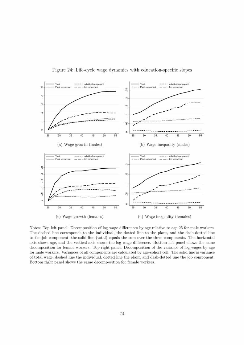
Figure 24: Life-cycle wage dynamics with education-specific slopes

0.1

.2.3

.4.5

25 30 35 40 45 50 55

Total Individual component

Plant component Job component

(a) Wage growth (males)

0.0

5.1

.15

.2.2

5

25 30 35 40 45 50 55

Total Individual component

Plant component Job component

(b) Wage inequality (males)

0.0

5.1

.15

.2.2

5

25 30 35 40 45 50 55

Total Individual component

Plant component Job component

(c) Wage growth (females)

0.0

5.1

.15

.2

25 30 35 40 45 50 55

Total Individual component

Plant component Job component

(d) Wage inequality (females)

Notes: Top left panel: Decomposition of log wage differences by age relative to age 25 for male workers.The dashed line corresponds to the individual, the dotted line to the plant, and the dash-dotted lineto the job component; the solid line (total) equals the sum over the three components. The horizontalaxis shows age, and the vertical axis shows the log wage difference. Bottom left panel shows the samedecomposition for female workers. Top right panel: Decomposition of the variance of log wages by agefor male workers. Variances of all components are calculated by age-cohort cell. The solid line is varianceof total wage, dashed line the individual, dotted line the plant, and dash-dotted line the job component.Bottom right panel shows the same decomposition for female workers.

74

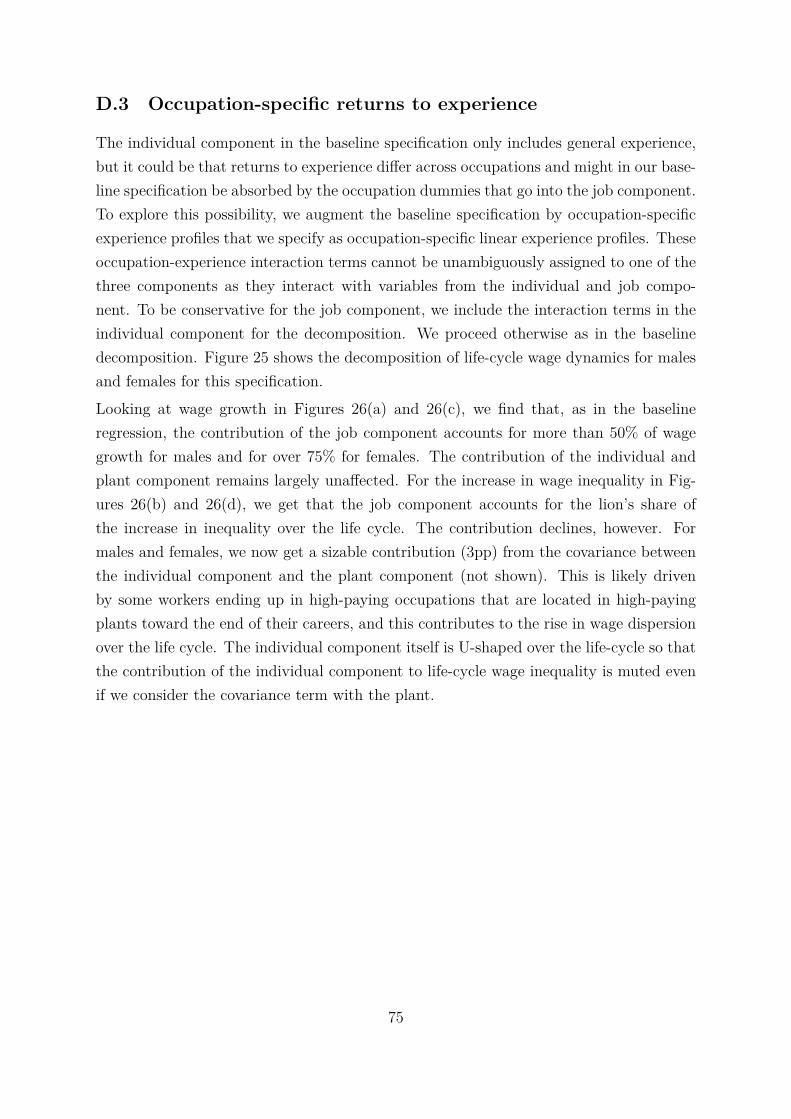
D.3 Occupation-specific returns to experience

The individual component in the baseline specification only includes general experience,but it could be that returns to experience differ across occupations and might in our base-line specification be absorbed by the occupation dummies that go into the job component.To explore this possibility, we augment the baseline specification by occupation-specificexperience profiles that we specify as occupation-specific linear experience profiles. Theseoccupation-experience interaction terms cannot be unambiguously assigned to one of thethree components as they interact with variables from the individual and job compo-nent. To be conservative for the job component, we include the interaction terms in theindividual component for the decomposition. We proceed otherwise as in the baselinedecomposition. Figure 2525 shows the decomposition of life-cycle wage dynamics for malesand females for this specification.Looking at wage growth in Figures 26(a)26(a) and 26(c)26(c), we find that, as in the baselineregression, the contribution of the job component accounts for more than 50% of wagegrowth for males and for over 75% for females. The contribution of the individual andplant component remains largely unaffected. For the increase in wage inequality in Fig-ures 26(b)26(b) and 26(d)26(d), we get that the job component accounts for the lion’s share ofthe increase in inequality over the life cycle. The contribution declines, however. Formales and females, we now get a sizable contribution (3pp) from the covariance betweenthe individual component and the plant component (not shown). This is likely drivenby some workers ending up in high-paying occupations that are located in high-payingplants toward the end of their careers, and this contributes to the rise in wage dispersionover the life cycle. The individual component itself is U-shaped over the life-cycle so thatthe contribution of the individual component to life-cycle wage inequality is muted evenif we consider the covariance term with the plant.

75

Figure 25: Decomposition of life-cycle wage dynamics with occupation-specific experience

0.1

.2.3

.4.5

25 30 35 40 45 50 55

Total Individual component

Plant component Job component

(a) Wage growth (males)

0.0

5.1

.15

.2.2

5

25 30 35 40 45 50 55

Total Individual component

Plant component Job component

(b) Wage inequality (males)

0.0

5.1

.15

.2.2

5

25 30 35 40 45 50 55

Total Individual component

Plant component Job component

(c) Wage growth (females)

0.0

5.1

.15

.2

25 30 35 40 45 50 55

Total Individual component

Plant component Job component

(d) Wage inequality (females)

Notes: Top left panel: Decomposition of log wage differences by age relative to age 25 for male workers.The dashed line corresponds to the individual, the dotted line to the plant, and the dash-dotted lineto the job component; the solid line (total) equals the sum over the three components. The horizontalaxis shows age, and the vertical axis shows the log wage difference. Bottom left panel shows the samedecomposition for female workers. Top right panel: Decomposition of the variance of log wages by agefor male workers. Variances of all components are calculated by age-cohort cell. The solid line is varianceof total wage, dashed line the individual, dotted line the plant, and dash-dotted line the job component.Bottom right panel shows the same decomposition for female workers.

76

D.4 Returns to tenure

A large literature in labor economics explores whether workers’ wages rise with tenure.Seminal contributions to this literature are by Altonji and ShakotkoAltonji and Shakotko (19871987) and TopelTopel(19911991). Our baseline regression does not include tenure effects. As an extension, we allowfor tenure effects and add dummies for employer tenure to our baseline regression. Unlikelabor market experience, employer tenure is not transferable in the labor market and isclosely associated with the employer and current job. It also seems plausible that tenureis determined by career progression at the current employer so that it is the by-product ofa successful career. We therefore include the tenure effects in the job component for thedecomposition. We proceed otherwise as in the baseline decomposition. Figure 2626 showsthe decomposition of life-cycle wage dynamics for males and females for this specification.Looking at wage growth in Figures 27(a)27(a) and 27(c)27(c), we find an even larger contribution ofthe job component to wage growth than in our baseline specification. For males, the jobcomponent now accounts for almost 80% of wage growth and for females for the entirewage growth over the life cycle. If we decompose the job component, we find that thejob-level component accounts for two-thirds of the job component for males and for 40%for females (not shown). Results for the variance remain largely unaffected (Figures 27(b)27(b)and 27(d)27(d)). Including the covariances (not shown), we again find that the job componentaccounts for the entire increase in wage inequality over the life cycle.

77

Figure 26: Life-cycle wage dynamics with occupation-specific slopes

0.1

.2.3

.4.5

25 30 35 40 45 50 55

Total Individual component

Plant component Job component

(a) Wage growth (males)

0.0

5.1

.15

.2.2

5

25 30 35 40 45 50 55

Total Individual component

Plant component Job component

(b) Wage inequality (males)

0.0

5.1

.15

.2.2

5

25 30 35 40 45 50 55

Total Individual component

Plant component Job component

(c) Wage growth (females)

0.0

5.1

.15

.2

25 30 35 40 45 50 55

Total Individual component

Plant component Job component

(d) Wage inequality (females)

Notes: Top left panel: Decomposition of log wage differences by age relative to age 25 for male workers.The dashed line corresponds to the individual, the dotted line to the plant, and the dash-dotted lineto the job component; the solid line (total) equals the sum over the three components. The horizontalaxis shows age, and the vertical axis shows the log wage difference. Bottom left panel shows the samedecomposition for female workers. Top right panel: Decomposition of the variance of log wages by agefor male workers. Variances of all components are calculated by age-cohort cell. The solid line is varianceof total wage, dashed line the individual, dotted line the plant, and dash-dotted line the job component.Bottom right panel shows the same decomposition for female workers.

78

D.5 Pooled regression without individual fixed effects

The main part of the paper uses synthetic cohorts to control for individual fixed effectsthat are arguably correlated with education, career progression, and potentially employertypes. In this section, we run as an alternative specification a pooled OLS regressioncontrolling for cohort effects but not controlling for individual fixed effects. Specifically,we set γi = γc in equation (22) and instead run the following regression on the pooleddata:

wit = γc + βJ Jit + βI Iit + ϵit. (5)

We proceed otherwise as described in the main part of the paper and use the same controlvariables for the job component Jit and individual component Iit. We again also demeanat the plant level to construct Jit and Iit. Figure 2727 shows the decomposition of wagegrowth in the individual, plant, and job component if we do not control for individualfixed effects.

Figure 27: Wage decomposition for males and females without controlling for individualfixed effects

0.1

.2.3

.4.5

25 30 35 40 45 50 55

Total Individual component

Plant component Job component

(a) Males

0.0

5.1

.15

.2.2

5

25 30 35 40 45 50 55

Total Individual component

Plant component Job component

(b) Females

Notes: Decomposition of log wage differences by age relative to age 25 for male (left panel) and female(right panel) workers. Decomposition based on regression without controls for individual fixed effects.The dashed line corresponds to the individual, the dotted line to the plant, and the dashed-dotted lineto the job component; the solid line (total) equals the sum over the three components. The horizontalaxis shows age, and the vertical axis shows the log wage difference. As in the main text, all graphs showthe coefficients of age dummies of a regression of the components on a full set of age and cohort dummies(ages defined as three-year groups).

Comparing the decomposition results for wage growth to the baseline results in Figure 11shows that the key finding of the importance of the job component for wage growth overthe life cycle is robust. We find that for both males and females, the contribution of thejob component to wage growth is still most important if we do not control for individualfixed effects. If individual fixed effects are important for labor market outcomes, we

79

should expect that estimated coefficients change from omitting this control variable fromthe regression. We find a sizable effect on the individual and plant components, which weinterpret as an omitted variable bias from the individual fixed effect. The result that thejob component is the driver of the increase in wage dispersion is also robust to omittingcontrols for individual fixed effects. We find that in the decomposition of the increase inwage dispersion, the contribution of covariances between the three components becomesmore important. We attribute these differences to the omitted individual fixed effect anddo not report the results here. These results are available from the authors upon request.

D.6 Residual variance

We show the decomposition of life-cycle wage dispersion for males and females in Fig-ures 44 and 55. The wage decomposition contains a residual that is by construction zeroon average conditional on age, but it might have an age-varying variance. A com-mon approach to modeling wage dynamics interprets these residuals as the realizationof wage risk (Lillard and WillisLillard and Willis (19781978), MaCurdyMaCurdy (19821982), Carroll and SamwickCarroll and Samwick (19971997),Meghir and PistaferriMeghir and Pistaferri (20042004), and GuvenenGuvenen (20092009)). Increasing the life-cycle profiles ofthe residual variance is, through the lens of this approach, interpreted as a stochasticprocess with a large and strongly persistent shock component, in the limiting case, evenfully persistent. Figure 2828 shows the variance of residuals from our decomposition. Wefind a small increase of less than 5 log points for males and virtually no increase forfemales. The very modest increase in the variance by age would be interpreted in theexisting literature as providing little evidence for large and persistent wage shocks andthat wage fluctuations over the life cycle are few and transitory.

80

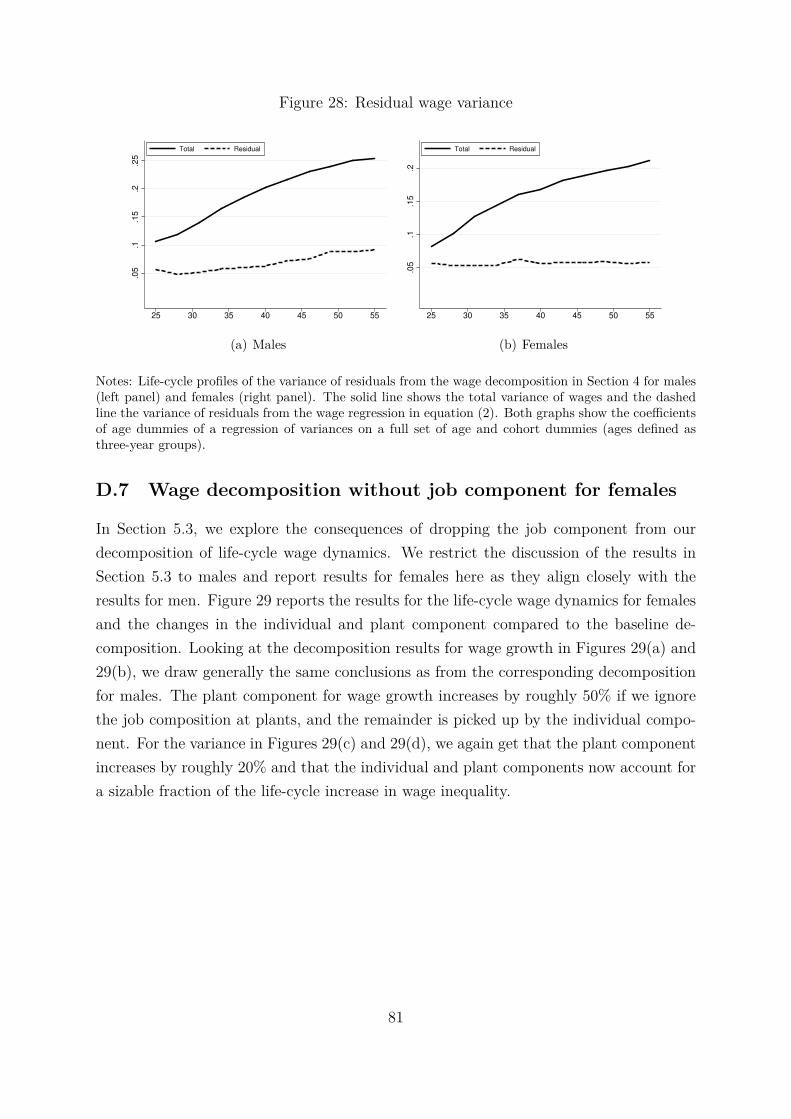
Figure 28: Residual wage variance

.05

.1.1

5.2

.25

25 30 35 40 45 50 55

Total Residual

(a) Males

.05

.1.1

5.2

25 30 35 40 45 50 55

Total Residual

(b) Females

Notes: Life-cycle profiles of the variance of residuals from the wage decomposition in Section 44 for males(left panel) and females (right panel). The solid line shows the total variance of wages and the dashedline the variance of residuals from the wage regression in equation (22). Both graphs show the coefficientsof age dummies of a regression of variances on a full set of age and cohort dummies (ages defined asthree-year groups).

D.7 Wage decomposition without job component for females

In Section 5.35.3, we explore the consequences of dropping the job component from ourdecomposition of life-cycle wage dynamics. We restrict the discussion of the results inSection 5.35.3 to males and report results for females here as they align closely with theresults for men. Figure 2929 reports the results for the life-cycle wage dynamics for femalesand the changes in the individual and plant component compared to the baseline de-composition. Looking at the decomposition results for wage growth in Figures 2929(a) and2929(b), we draw generally the same conclusions as from the corresponding decompositionfor males. The plant component for wage growth increases by roughly 50% if we ignorethe job composition at plants, and the remainder is picked up by the individual compo-nent. For the variance in Figures 2929(c) and 2929(d), we again get that the plant componentincreases by roughly 20% and that the individual and plant components now account fora sizable fraction of the life-cycle increase in wage inequality.

81

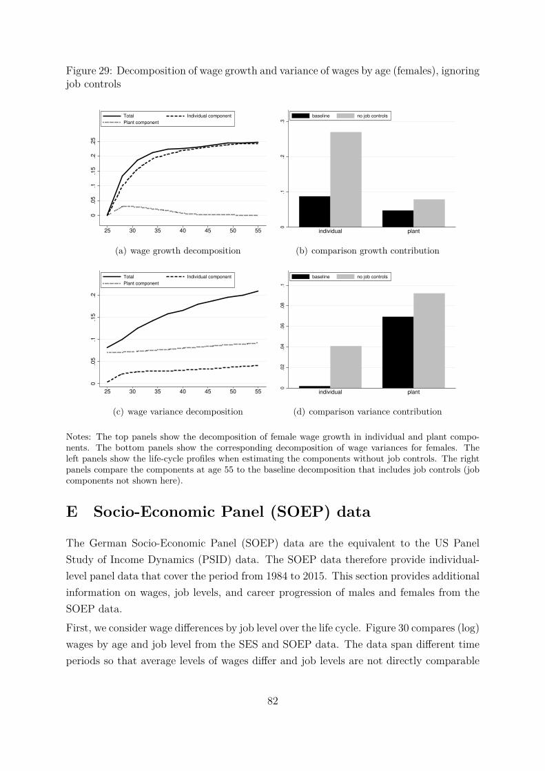
Figure 29: Decomposition of wage growth and variance of wages by age (females), ignoringjob controls

0.0

5.1

.15

.2.2

5

25 30 35 40 45 50 55

Total Individual component

Plant component

(a) wage growth decomposition

0.1

.2.3

individual plant

baseline no job controls

(b) comparison growth contribution

0.0

5.1

.15

.2

25 30 35 40 45 50 55

Total Individual component

Plant component

(c) wage variance decomposition

0.0

2.0

4.0

6.0

8.1

individual plant

baseline no job controls

(d) comparison variance contribution

Notes: The top panels show the decomposition of female wage growth in individual and plant compo-nents. The bottom panels show the corresponding decomposition of wage variances for females. Theleft panels show the life-cycle profiles when estimating the components without job controls. The rightpanels compare the components at age 55 to the baseline decomposition that includes job controls (jobcomponents not shown here).

E Socio-Economic Panel (SOEP) data

The German Socio-Economic Panel (SOEP) data are the equivalent to the US PanelStudy of Income Dynamics (PSID) data. The SOEP data therefore provide individual-level panel data that cover the period from 1984 to 2015. This section provides additionalinformation on wages, job levels, and career progression of males and females from theSOEP data.First, we consider wage differences by job level over the life cycle. Figure 3030 compares (log)wages by age and job level from the SES and SOEP data. The data span different timeperiods so that average levels of wages differ and job levels are not directly comparable

82

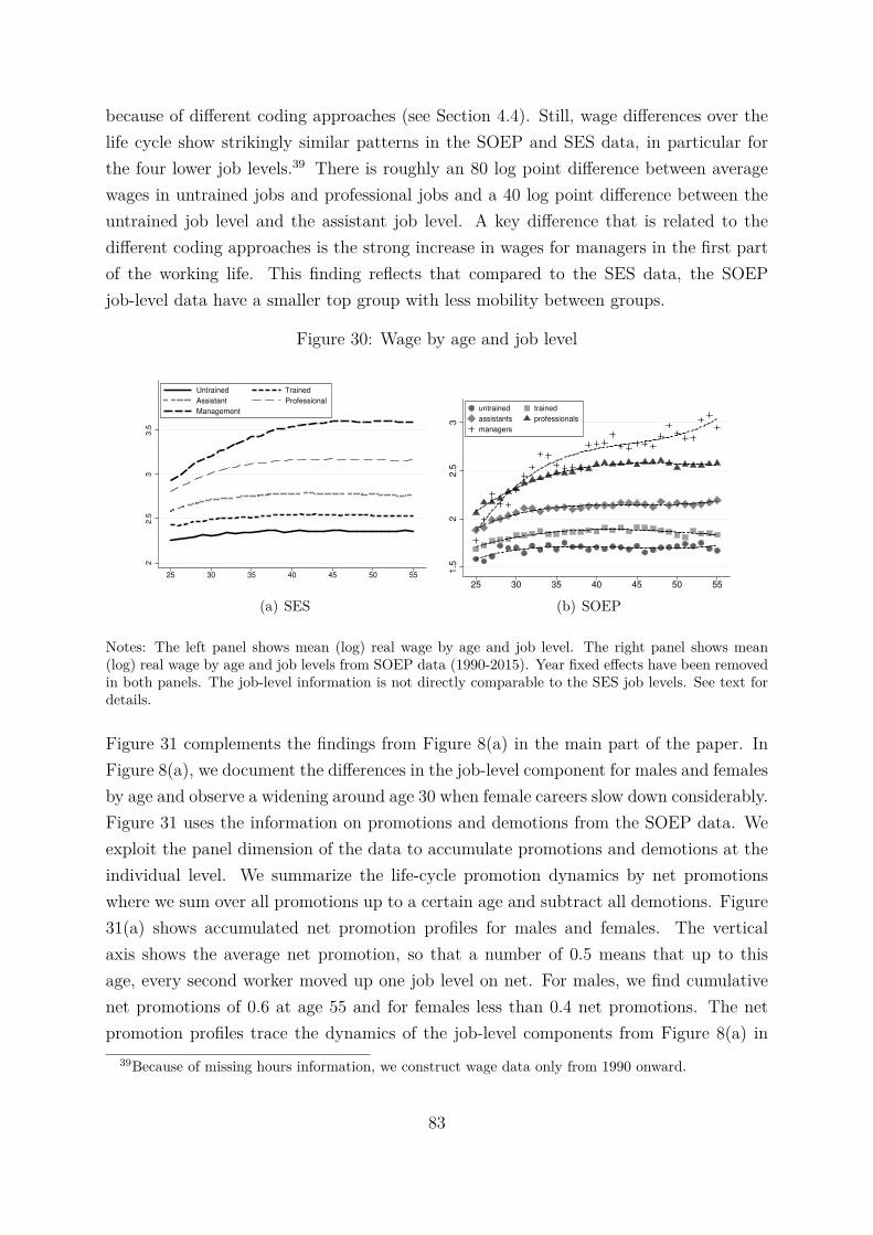
because of different coding approaches (see Section 4.44.4). Still, wage differences over thelife cycle show strikingly similar patterns in the SOEP and SES data, in particular forthe four lower job levels.3939 There is roughly an 80 log point difference between averagewages in untrained jobs and professional jobs and a 40 log point difference between theuntrained job level and the assistant job level. A key difference that is related to thedifferent coding approaches is the strong increase in wages for managers in the first partof the working life. This finding reflects that compared to the SES data, the SOEPjob-level data have a smaller top group with less mobility between groups.

Figure 30: Wage by age and job level

22.5

33.5

25 30 35 40 45 50 55

Untrained Trained

Assistant Professional

Management

(a) SES

1.5

22

.53

25 30 35 40 45 50 55age

untrained trained

assistants professionals

managers

(b) SOEP

Notes: The left panel shows mean (log) real wage by age and job level. The right panel shows mean(log) real wage by age and job levels from SOEP data (1990-2015). Year fixed effects have been removedin both panels. The job-level information is not directly comparable to the SES job levels. See text fordetails.

Figure 3131 complements the findings from Figure 88(a) in the main part of the paper. InFigure 88(a), we document the differences in the job-level component for males and femalesby age and observe a widening around age 30 when female careers slow down considerably.Figure 3131 uses the information on promotions and demotions from the SOEP data. Weexploit the panel dimension of the data to accumulate promotions and demotions at theindividual level. We summarize the life-cycle promotion dynamics by net promotionswhere we sum over all promotions up to a certain age and subtract all demotions. Figure3131(a) shows accumulated net promotion profiles for males and females. The verticalaxis shows the average net promotion, so that a number of 0.5 means that up to thisage, every second worker moved up one job level on net. For males, we find cumulativenet promotions of 0.6 at age 55 and for females less than 0.4 net promotions. The netpromotion profiles trace the dynamics of the job-level components from Figure 88(a) in

39Because of missing hours information, we construct wage data only from 1990 onward.

83

the main part of the paper; in particular, we observe a strong slowdown of promotiondynamics for females after age 30. Figure 3131(b) shows the difference in net promotionsfor males and females. Unlike for the job-level component from Figure 88(a), we alreadysee a widening of promotion dynamics at age 25 that continues up to age 40 when thedifference in net promotion stabilizes at about 0.25. This implies that every fourth netpromotion for males is not taking place for females and that this difference arises in thefirst half of the working life. However, one should also take into account that the SESdata and the SOEP data cover different survey years.

Figure 31: Cumulated net promotions and demotions by age

0.2

.4.6

25 30 35 40 45 50 55age

males females

(a) Cumulated net promotions

0.1

.2.3

25 30 35 40 45 50 55age

(b) Differential cumulated net promotions

Notes: The figures display the accumulated net promotion rates for male and female workers from theSOEP data (1984-2015) and their differences across gender by age.

84