Which inflation to target? A small open economy withsticky wages indexed to past inflation∗

Alessia Campolmi†

November 4, 2006

Abstract

There is common agreement on price inflation stabilization being one of the ob-jectives of monetary policy. But, in an open economy, two alternative measures ofinflation coexist: domestic inflation (DI) and consumer price inflation (CPI). Whichone of the two should be the target variable? Most of the literature suggests that themonetary authority should try to stabilize DI. This is in sharp contrast with the prac-tice of many inflation-targeting central banks which are using CPI as target variable. Iuse a small open economy model to show that CPI targeting can be rationalized by thepresence of sticky wages indexed to past CPI. The latter assumption is highly plausible,as documented by the empirical evidence reported in, e.g., Smets and Wouters (2003).

After deriving the welfare function from a second order approximation of the utilityfunction, I compute the fully optimal monetary policy under commitment and use itas a benchmark to compare the performance of different monetary policy rules. Therule performing best is the one targeting wage inflation and CPI. Moreover, this ruledelivers results very close to those obtained under the fully optimal monetary policywith commitment.JEL Classification: E52, F41Keywords: inflation, open economy, sticky wages, indexation, optimal monetary policy.

∗I would like to thank Jordi Galı for excellent supervision. I also thank Ester Faia, Michael Reiter, StefanoGnocchi, Chiara Forlati, Harald Fadinger, Albi Tola, Alessandro Flamini and participants at the EEA2006 conference, the SMYE 2005 conference, and seminar participants at Universitat Pompeu Fabra, DukeUniversity, Univerista di Milano-Bicocca and Universita di Bologna for helpful comments and suggestions.I gratefully acknowledge financial support from Marco Polo grant of Univerista di Bologna. All errors aremine.

†Department of Economics, Universitat Pompeu Fabra, Ramon Trias Fargas, 25, 08005 Barcelona, Spain,alessia.campolmi@upf.edu and Universita di Bologna, Italy. Personal Home Page: www.econ.upf.edu/∼campolmi/

1

1 Introduction

The purpose of the present paper is to analyse which measure of inflation shouldbe chosen as target variable in an open economy framework. In a closed economycontext there is common agreement on price inflation stabilization being one of themain objectives of monetary policy. From the ad-hoc interest rate rule proposed byTaylor (1993), to the more recent New Keynesian literature deriving optimal monetarypolicy rules from the minimization of a microfounded loss function, the monetaryinstrument has to be chosen in order to match a given inflation target (among withother targets). However, in an open economy context two alternative measures ofinflation coexist: Domestic Inflation (DI) and Consumer Price Inflation (CPI). Whichone of these two should be the target variable? This is the question addressed in thepaper.

With this purpose in mind, I develop a small open economy model similar to the oneused by Galı and Monacelli (2005). The main difference with respect to the existingopen economy literature is that, in addition to the standard hypothesis of sticky prices,I assume sticky wages. I also allow for a partial indexation to past CPI. In each periodonly a fraction of workers reoptimize while the others partially index their nominalwages to past CPI. Under those assumptions, the volatility of CPI and the impossibilityfor some workers to adjust their wages in order to keep their mark-ups constant makethe stabilization of CPI relevant in this context. In particular, the assumption on wageshas two main consequences: first, given the presence of wage rigidities, strict inflationtargeting will no longer be optimal (as Erceg, Henderson and Levin (2000) show in aclosed economy setup); second, fluctuations in CPI will induce undesired fluctuationsin wage mark-ups and, therefore, in firms’ marginal costs and DI. The link betweenCPI and DI through firm’s marginal cost is further increased when there is a positivedegree of wage indexation.

The main result of the paper is that, reacting to changes in CPI instead of focusingon targeting DI, the monetary authority will obtain better results not only in thestabilization of CPI but also in that of wage inflation, DI, and output gap. This makesit desirable to stabilize CPI rather than DI. The importance of this result is that,differently from the existing open economy literature, it is in line with the practiceof inflation-targeting central banks. Indeed, from an operational point of view, thereseems to be an unanimous consensus among central banks on CPI being the correcttarget. In particular, as stressed by Bernanke and Mishkin (1997), starting from 1990the following countries have adopted an explicit target to CPI: Australia, Canada,Finland, Israel, New Zealand, Spain, Sweden, UK. In the EMU, the European CentralBank has the object to stabilize the Harmonized Index of Consumer Prices (HCPI)below 2%. In contrast, from a theoretical point of view, most of the literature suggeststhat the monetary authority should choose DI as target variable for inflation1. Hence,the contribution of the paper is to show that the introduction of sticky wages indexedto past inflation reconciles the workhorse model for monetary policy analysis in openeconomy with the practice of many monetary authorities.

1A detailed review of the related literature is provided in the next section.

2

Regarding the assumptions on which the results of the paper are built, there isstrong empirical evidence of wage rigidity in the economy2, as underlined by Christiano,Eichenbaum and Evans (2005) and by Smets and Wouters (2003). Moreover, Smetsand Wouters (2003) estimate the degree of wage indexation to past inflation for theEURO area to be around 0.65. The main conclusion of both Christiano et al. (2005)and Smets and Wouters (2003) is that the introduction of wage rigidity is a crucialassumption in order to improve the ability of the New-Keynesian models to matchthe data. Consequently, there is empirical evidence in favour of the importance ofmodelling also wage rigidity in order to obtain more reliable dynamics.

Solving the model under the assumption of sticky wages and looking at the PhillipsCurve and the wage inflation equation there emerges a link between DI, CPI and wageinflation. Given this link, it is clearly difficult to stabilize DI without stabilizing alsoCPI and wage inflation. In order to obtain a more precise analysis of what a centralbank should do, I derive the welfare function as a second order approximation of theutility function and I compute the fully optimal monetary policy under commitment.Using the optimal monetary policy as a benchmark, I then compare different, imple-mentable, monetary policy rules. In the choice of possible targets for monetary policy Idisregard the output gap because it cannot be considered a feasible target since it is notclear how to estimate the natural level of output. Therefore, I concentrate on the otherthree variables that appear in the loss function i.e., DI, CPI and wage inflation. I focuson interest rate rules targeting either just one or two of the three variables at the sametime. I simulate the model under these monetary policy rules and for different degreesof wage indexation in order to analyse how this feature of the model affects the results.If we consider rules targeting just one variable per time, the rule performing best isthe one targeting CPI, even when there is no wage indexation. The rule targeting DIperforms much worse in terms of welfare. The reason is that, targeting CPI insteadof DI, improves substantially the stabilization of all the main variables. Looking atrules targeting two variables at the same time, the first thing that emerges is thatcentral banks should use wage inflation as their second target variable. In the case ofno indexation, a rule targeting DI and wage inflation is almost undistinguishable fromone targeting CPI and wage inflation in terms of welfare. But, as soon as a positivedegree of indexation is introduced, the policy rule that gives the best results is the onetargeting both CPI and wage inflation. Increasing the level of indexation reinforcesthe results. Simulating the model under the optimal monetary policy rule and underthe interest rate rules and looking at the correlations among the series simulated inthe different scenarios, it is clear that the rule targeting at CPI and wage inflationdelivers a behaviour of the economy that is very close to the one obtained under thefully optimal rule.

These results therefore confirm the original hypothesis that the introduction of wagerigidity would have affected the ranking among policy rules giving more importance tothe stabilization of CPI, therefore rationalizing the observed behaviour of many centralbanks.

2For a review of the micro evidence of wage stickiness and of the importance of modelling wage rigiditiestogether with price rigidities see Taylor (1998).

3

The structure of the paper is the following: section 2 presents the related literature,section 3 introduces the open economy model, section 4 presents the analysis of thewelfare function, section 5 computes the optimal monetary policy under commitment,section 6 shows how different, implementable, monetary policy rules perform underdifferent degrees of indexation and section 7 concludes.

2 Related literature

Clarida, Galı and Gertler (2001) analyse a small open economy model with price rigidi-ties and frictions in the labour market. They find that, as long as there is perfectexchange rate pass-through, the target of the central bank should be DI. This is whatthey call ”the isomorphic result” meaning that the form of the optimal interest raterule is not affected by the consideration of being in an open economy. Openness onlyaffects the aggressiveness with which the central bank should react to shocks. There-fore, the central bank should target DI and not CPI. However, in their paper they donot explicitly model frictions in the labour market. They just assume an exogenousstochastic process for the wage mark-up. This is an important difference with respectto the model I develop because, even if assuming an exogenous process for the wagemark-up makes price stability no more optimal (like here), the link between fluctuationsin the wage mark-up and fluctuations in CPI is missing. A similar result is obtainedin Galı and Monacelli (2005)3 where strict DI targeting turns out to be the optimalmonetary policy, consequently outperforming a CPI targeting rule. Aoki (2001) showsthat in a two-sector closed economy with different price rigidities, more weight shouldbe attributed to the inflation of the stickier sector4. The extension of this result toa small open economy context implies that the monetary authority should target theDI. Clarida, Galı and Gertler (2002) show, in a two-country model with sticky pricesthat, in the case of no coordination, the two monetary authorities should adjust theinterest rate in response to DI. Benigno (2004) studies optimal monetary policy in acurrency area using a two-country model with monopolistic competition and stickyprices in both regions. There are two independent fiscal authorities while there is onlyone monetary authority. The result is a generalization of the one obtained by Aoki(2001) in the closed economy, two-sector model. In the special case where prices arerigid only in one country, the central bank should stabilize DI in the country with stickyprices. In a more general case, where prices are rigid in both countries and the degreeof price stickiness differs across the two regions, in the class of inflation targeting rules

3Under the assumptions of log utility in consumption and unit elasticity of substitution among foreigngoods.

4Another closed economy model dealing with which inflation variable to target is the one by Huang andLiu (2005). In their model there are two sectors, one for the production of intermediate goods and one forthe production of final goods. Intermediate goods are produced using labour as the only input while toproduce final goods labour is combined with the intermediate goods. Prices are rigid in both sectors andthere are sector specific shocks. The main conclusion is that an interest rate rule targeting both CPI andPPI (producer price inflation) would attain better results than one seeking to stabilize CPI. Anyway, asstressed by the authors in the paper, ”the PPI [...] does not have a clear counterpart in an open economysetup” making a comparison with an open economy model difficult.

4

where the target is a weighted average of the DI in the two countries, higher weightneeds to be attributed to the DI of the country with relatively more rigid prices. Still,as in the previous papers, the target variable is DI and not CPI.

Differently from the aforementioned papers, Corsetti and Pesenti (2005) and De-Paoli (2004) find that DI is not always the optimal target. But, the focus in thosepapers is not on which inflation to target but more on the general question of whetherthe policy should be inward-looking or outward-looking. Corsetti and Pesenti (2005)use a two-country model with firms’ prices set one period in advance and incompletepass-through to show that ”inward-looking policy of domestic price stabilization is notoptimal when firms’ markups are exposed to currency fluctuations”. DePaoli (2004)extends the welfare analysis for the small open economy of Galı and Monacelli (2005)allowing for a more general specification of the utility function and of the elasticity ofsubstitution among domestically produced and foreign goods and finds that the mone-tary authority should target also the exchange rate, therefore supporting an outward-looking monetary policy. A paper dealing directly with the question of whether themonetary authority should target DI or CPI is the one by Svensson (2000). He usesa small open economy framework to analyse inflation targeting monetary policies andhe underlines that ”all inflation-targeting countries have chosen to target CPI...Noneof them has chosen to target domestic inflation”. He assumes an ad-hoc loss functionthat includes both CPI and DI in addition to other variables. The result of the model(that is not fully microfounded) is that flexible CPI targeting is better than flexibleDI targeting. Also in Monacelli (2005), the monetary authority is assumed to targetCPI instead of DI, in order to behave like many central banks do in practice, but thewelfare function is not derived.

Summarizing, with the exception of the paper by Svensson (2000), that is not fullymicrofounded, the papers claiming for an outward-looking monetary policy do notdeal with the question of which measure of inflation should be chosen by the monetaryauthority. Here is where the contribution of the paper lies.

3 The model

Like in Galı and Monacelli (2005), there is a continuum [0, 1] of small, identical, coun-tries. Differently from the original model, I introduce the assumption of monopolisticcompetition on the supply side of the labour market. I also assume the presence ofwage rigidities. It is worthy to note that, since I assume complete markets and sep-arable utility, households differ in the amount of labour supplied (consequence of thepresence of sticky wages) but share the same consumption. I also keep the simplifyingassumption that the law of one price holds for individual goods at all times. Fromnow on I will use ”h” as index for a particular household, ”i” to refer to a particularcountry and ”j” as sector index. When no index is specified the variables refer to thehome country.

5

3.1 Households

Household ”h” maximizes:

E0

∞∑t=0

βt [U(Ct) + V (Nt(h))] (1)

where Nt(h) is the labour supply and Ct is a consumption index which aggregatebundles of domestic and imported goods:

Ct ≡[(1− α)

1η C

η−1η

H,t + α1η C

η−1η

F,t

] ηη−1

(2)

where α represents the degree of openness, and CH,t and CF,t are two aggregate con-sumption indices, respectively for domestic and imported goods:

CH,t ≡

1∫0

CH,t(j)θp−1

θp dj

θp

θp−1

(3)

CF,t ≡

1∫0

Cη−1

η

i,t di

η

η−1

(4)

Ci,t ≡

1∫0

Ci,t(j)θp−1

θp dj

θp

θp−1

(5)

The parameter θp > 1 represents the elasticity of substitution between two varietiesof goods produced in the same country, while the parameter η > 0 represents theelasticity of substitution between home produced goods and goods produced abroad.Each household h maximizes (1) subject to a sequence of budget constraints. Theresults regarding the optimal allocation of expenditure across goods are not affectedby the introduction of monopolistic competition in the labour market, so using theresults of Galı and Monacelli (2005), I can directly write the budget constraint afterhaving aggregated over goods:

PtCt + Et [Qt,t+1Dt+1] ≤ Dt + (1 + τw)Wt(h)Nt(h) + Tt (6)

where Qt,t+1 is the stochastic discount factor, Dt is the payoff in t of the portfolioheld at the end of t− 1, Tt is a lump-sum transfer (or tax) which also includes profitsresulting from ownership of firms, τw is a subsidy to labour income and Pt is theaggregate price index:

Pt ≡[(1− α)(PH,t)1−η + α(PF,t)1−η

] 11−η (7)

PH,t ≡[∫ 1

0PH,t(j)1−θpdj

] 11−θp

(8)

6

PF,t ≡[∫ 1

0P 1−η

i,t di

] 11−η

(9)

Pi,t ≡[∫ 1

0Pi,t(j)1−θpdj

] 11−θp

(10)

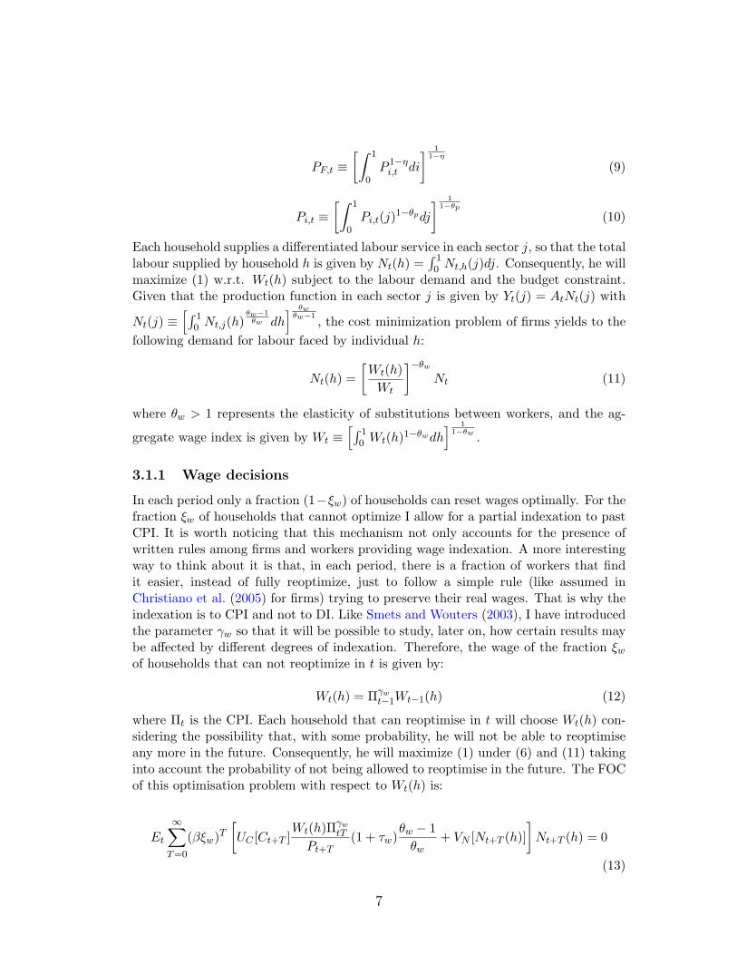
Each household supplies a differentiated labour service in each sector j, so that the totallabour supplied by household h is given by Nt(h) =

∫ 10 Nt,h(j)dj. Consequently, he will

maximize (1) w.r.t. Wt(h) subject to the labour demand and the budget constraint.Given that the production function in each sector j is given by Yt(j) = AtNt(j) with

Nt(j) ≡[∫ 1

0 Nt,j(h)θw−1

θw dh] θw

θw−1, the cost minimization problem of firms yields to the

following demand for labour faced by individual h:

Nt(h) =[Wt(h)

Wt

]−θw

Nt (11)

where θw > 1 represents the elasticity of substitutions between workers, and the ag-

gregate wage index is given by Wt ≡[∫ 1

0 Wt(h)1−θwdh] 1

1−θw .

3.1.1 Wage decisions

In each period only a fraction (1−ξw) of households can reset wages optimally. For thefraction ξw of households that cannot optimize I allow for a partial indexation to pastCPI. It is worth noticing that this mechanism not only accounts for the presence ofwritten rules among firms and workers providing wage indexation. A more interestingway to think about it is that, in each period, there is a fraction of workers that findit easier, instead of fully reoptimize, just to follow a simple rule (like assumed inChristiano et al. (2005) for firms) trying to preserve their real wages. That is why theindexation is to CPI and not to DI. Like Smets and Wouters (2003), I have introducedthe parameter γw so that it will be possible to study, later on, how certain results maybe affected by different degrees of indexation. Therefore, the wage of the fraction ξw

of households that can not reoptimize in t is given by:

Wt(h) = Πγwt−1Wt−1(h) (12)

where Πt is the CPI. Each household that can reoptimise in t will choose Wt(h) con-sidering the possibility that, with some probability, he will not be able to reoptimiseany more in the future. Consequently, he will maximize (1) under (6) and (11) takinginto account the probability of not being allowed to reoptimise in the future. The FOCof this optimisation problem with respect to Wt(h) is:

Et

∞∑T=0

(βξw)T

[UC [Ct+T ]

Wt(h)Πγw

tT

Pt+T(1 + τw)

θw − 1θw

+ VN [Nt+T (h)]]

Nt+T (h) = 0

(13)

7

with ΠtT = ΠtΠt+1....ΠT−1 = Pt+T−1

Pt−1. From (13) it is clear that the solution Wt(h)

will be the same for all households that are allowed to reoptimise in t. To solve for theoptimal wage we need first to log linearize (13) around the steady state:

Et

∞∑T=0

(βξw)T[Ψt+T − MRSt+T (h)

]= 0 (14)

where Ψt+T = WtΠγwtT

Pt+Tis the real wage, MRSt = −VN,t

UC,tand Ψt+T and MRSt+T (h) are

the log deviations from their levels with flexible prices. Rearranging terms I get thefollowing equation for the optimal wage:

log Wt = −log(1−Φw)+(1−βξw)Et

∞∑T=0

(βξw)T [log MRSt+T (h) + log Pt+T − γw log ΠtT ]

(15)where log(1 − Φw) = log(1 + τw) − log(µw) and µw = θw

θw−1 is the wage markup.Whenever τw = 1

θw−1 , then Φw = 0 and the fiscal policy completely eliminates thedistortion caused by the presence of monopolistic competition in the supply of labour.When instead τw < 1

θw−1 , then − log(1 − Φw) > 0 and a distortion is present in theeconomy5. From now on the following specification for the utility function will beassumed:

U(C) + V (N) =C1−σ

1− σ− N1+ϕ

1 + ϕ(16)

where σ represents the relative risk aversion coefficient while ϕ is the inverse of thelabour supply elasticity. Given this specification, and with some algebra, it is possibleto derive the following expression:

log Wt =

−(1− βξw)1 + ϕθw

∞∑T=0

(βξw)T Et[µw,t+T ] + log(Wt) +

+∞∑

T=1

(βξw)T Et log Πw,t+T +

−γw(1− βξw)∞∑

T=0

(βξw)T Et log ΠtT (17)

where µw,t = log(Wt)− log(Pt)− log(MRSt)+log(1−Φw) represents the fluctuation inthe wage markup. The optimal wage today will be higher the higher the expectations

5Note that if θw

θw−1 = 1 + τw the fiscal policy is able to completely eliminate the distortion arising fromlabour markets. Following Woodford (2003) I define 1 − Φw = (1 + τw) θw−1

θw, where Φw represents the

distortion in the economy. Whenever Φw > 0 the level of employment in the flexible price equilibrium willbe lower than the one that we would have without distortions. When doing welfare analysis I will assumefor simplicity Φw = 0 but now I can consider the more general case.

8

about future wages. Future CPI has instead a negative impact because of indexation.In particular, the higher the level of indexation and the higher the expected futureCPI, the lower will be the optimal wage today. This is because agents know that evenif they will not be allowed to reoptimise in the near future, their wages will increaseanyway because of indexation. This effect would disappear with γ = 0. Note that,with the labour subsidy in place, the distortion in the labour market is smaller thanthe one that we would have without subsidy, indeed − log(µw) < log(1−Φw) ≤ 0. Still,µw,t = 0 means that the wage charged is higher then the one that would be chargedwith perfect competition on the labour market. So, even if the monetary authoritymanages to eliminate the distortions arising from the nominal rigidities, the level ofemployment will be lower then the natural one, unless Φw = 0.

The next step is to analyse the wage inflation equation. Given that the fraction(1 − ξw) of households that is allowed to reoptimise will choose the same wage, whilethe others will follow the indexation rule, the aggregate wage index is:

Wt =[(1− ξw)W 1−θw

t + ξw(Wt−1Πγwt−1)

1−θw

] 11−θw (18)

The log linearized version of this equation is given by:

logWt = (1− ξw) log Wt + ξw log Wt−1 + γwξw log Πt−1 (19)

It is useful to rewrite (17) in the following way:

logWt − βξwEt log Wt+1 = −1− βξw

1 + ϕθwµw,t + (1− βξw) log Wt (20)

From now on all the lower case letters denote the log of the variables. Combining (20)with (19) gives:

πw,t = −λwµw,t + βEt[πw,t+1]− ξwγwβπt + γwπt−1 (21)

where λw = 1−ξw

ξw

1−βξw

1+ϕθw. As in the case of no indexation, current wage inflation depends

positively on the expected future wage inflation and negatively on the deviation of themarkup from its frictionless level. In particular when µw,t > 0 the markup charged ishigher than its optimal level and that is way wages respond negatively to a positive µw,t.This result is consistent with the one obtained in Galı (2003) in the closed economycase with no indexation. The presence of indexation introduces two new elements: anegative impact of current CPI and a positive impact of past CPI. For what concernpresent inflation, because of indexation households know that, even if they will notbe able to change wages in the next period, their wages will increase because of thelink with current inflation, so there is no need to increase them today. Past inflation,instead, has a positive impact on current wage inflation because agents that are notallowed to reoptimize in t will see their wages increase because of indexation. In caseof no indexation, fluctuations in CPI will induce fluctuations in wage inflation onlythrough their impact on the wage mark-up.

Having discussed the wage decisions, I move to the consumption choice which isstandard.

9

3.1.2 Consumption Decisions

Maximizing (1) with respect to consumption and asset holdings subject to (6), leadsto the standard Euler Equation:

βRtEt

[(Ct+1

Ct

)−σ Pt

Pt+1

]= 1 (22)

with Rt = 1Et[Qt,t+1] .

3.2 Firms

The production function of a domestic firm in sector j is given by:

Yt(j) = AtNt(j) (23)

with at ≡ log(At) and

at+1 = ρaat + εA,t. (24)

where εA,t is an i.i.d shock with zero mean. The aggregate domestic output is givenby:

Yt =[∫ 1

0Yt(j)

θp−1

θp dj

] θpθp−1

(25)

Up to a first order approximation Galı and Monacelli (2005) demonstrate that:

yt = at + nt (26)

In each period only a fraction (1− ξp) of firms can reset prices optimally.Given that the elasticity of substitution between varieties of final goods is θp > 1,

the markup that each firm would like to charge is µp = θp

θp−1 . Assuming the presenceof a subsidy τp to the firm’s output, optimal price-setting of a home firm j must satisfythe following FOC:

Et

∞∑T=0

ξTp Qt,t+T Yt+T (j)

[(1 + τp)

θp − 1θp

PH,t(j)−MCt+T

]= 0 (27)

where MCt represents the nominal marginal cost. Like for wages, it is useful to define1 − Φp ≡ (1 + τp)

θp−1θp

, where Φp indicates the distortion due to monopoly power onthe firm side that is still present in the economy after the intervention of the fiscalauthority. If the fiscal authority optimally chooses τp in order to exactly offset themonopoly distortion then Φp = 0. If Φw > 0 and/or Φp > 0 then the flexible priceallocation will deliver an output and an employment level lower then the natural ones.

10

From the log-linear approximation of (27) around the steady state it is possible toderive the standard log-linear optimal price-setting rule:

pH,t = − log(1− Φp) + (1− βξp)Et

∞∑T=0

(βξp)T [mct+T + pH,t] (28)

where pH,t represents the (log) price chosen by the firms that are allowed to reoptimisein t, and mct represents the (log) real marginal cost.

3.3 Equilibrium Conditions

To close the model some relations between home and foreign variables are needed. A”star” will be used to denote world variables. The derivation of the following equations6

can be found in Galı and Monacelli (2005):

C∗t = Y ∗t (29)

ct = c∗t +1− α

σst (30)

where St ≡PF,t

PH,tare the effective terms of trade and (30) represents the international

risk sharing condition. The market clearing condition is given by:

Yt = CtSαt (31)

The world output is assumed to follow an exogenous law of motion:

y∗t+1 = ρyy∗t + εy,t. (32)

with εy,t i.i.d. shock with zero mean. The terms of trade can be expressed also infunction of the aggregate and the home price indexes:

αst = pt − pH,t (33)

The relation between the home output and the world output is given by:

st = σα(yt − y∗t ) (34)

with σα ≡ σ1−α+αω > 0 and ω ≡ ση + (1− α)(ση − 1).

6All these relations, with the only exception of (29) that is an exact relation, hold exactly only under theassumption that σ = η = 1. Otherwise they hold up to a first order approximation.

11

3.4 The New Keynesian Phillips Curve (NKPC)

The relation between DI and real marginal cost is not affected by the presence of stickywages:

πH,t = βEt[πH,t+1] + λmct (35)

with λ ≡ (1−βξp)(1−ξp)ξp

and with mct denoting log deviations of the real marginalcost from its level in the absence of nominal rigidities (i.e. mct = mct − mc withmc = log(1 − Φp)). The presence of sticky wages leads to an additional term in thestandard equation relating the marginal cost with the output gap (the derivation canbe found in the appendix):

mct = (σα + ϕ)(yt − yt) + µw,t (36)

When wages are fully flexible µw,t = 0. When wages are sticky this is no longer trueand in particular, when µw,t > 0, the markup charged by workers is higher than theoptimal one and firms bear a higher real marginal cost. Consequently the NKPC fora small open economy with both price and wage rigidities is:

πH,t = βEt[πH,t+1] + λ(σα + ϕ)(yt − yt) + λµw,t (37)

Even assuming that the only distortions left in the economy are the ones generatedby the presence of nominal rigidities, clearly, as in Erceg et al. (2000), since it is notpossible to stabilize at the same time DI, wage inflation and output gap, the flexibleprice allocation is no longer a feasible target. Is it still true then, that a Taylor ruletargeting DI is the one that performs best? It is interesting to analyse the impact ofan increase in pt on πH,t. To keep the wage markup constant wages should increaseto offset the change in prices but, because of stickiness, this is not possible for allhouseholds, so some of them will charge a wage that is lower than the desired one andµw,t will become negative. This will have a negative impact on DI. On the other hand,because of indexation to past inflation, in t + 1 the aggregate wage index will increaseand so will µw,t+1. This will lead to an increase of EtπH,t+1. So, other things equal,an increase in pt will cause an increase of πH,t+1, whereas the impact on current DIis not clear. Given this link between DI, CPI and wage inflation, it seems reasonableto postulate that targeting only one of these variables may not be optimal because, ifCPI and wage inflation are very volatile, it will be hard to stabilize only DI.

To prove this conjecture, in the next section, I derive the welfare function from asecond order approximation of the utility of the representative household. I then usethe welfare function to study the behavior of the economy under optimal monetarypolicy. Finally, using the results under optimal monetary policy as benchmark, Icompare different welfare losses obtained using different, implementable, policy rules.

4 Welfare function

Before starting with the welfare analysis it is important to underline that in the openeconomy model there are 5 distortions: monopolistic power in both goods and labour

12

markets; nominal rigidities in both wages and prices; incentives to generate an exchangerate appreciation. In a closed economy framework it is enough to require Φw = Φp = 0to ensure that the flexible price allocation will coincide with the optimal one, but thisis no more true in an open economy. As emphasised by Corsetti and Pesenti (2001),a monetary expansion has two consequences in this context: it increases the demandfor domestically produced goods and it deteriorates the terms of trade of domesticconsumers. So in some cases the monetary authority may have the incentive to generatean exchange rate appreciation, even at the cost of a level of output (employment)lower than the optimal one. From now on I will assume σ = η = 1 (i.e. log utilityin consumption and unit elasticity of substitution between home produced goods andgoods produced abroad). In this case the equilibrium conditions derived in 3.3 holdexactly and maximizing (1) under the production function Yt = AtNt, (30) and (31)leads to the following FOC:

− UN

UC= (1− α)A1−αN−α(Y ∗)α (38)

The solution is a constant, optimal, level of employment N = (1 − α)1

1+ϕ . Let usnow analyse under which conditions the flexible price equilibrium delivers the optimalallocation. Under flexible prices, in every period µw,t = mct = 0. Combining these twoconditions together with the equilibrium conditions, it is possible to derive:

N1+ϕt

µw

1 + τw=

1 + τp

µp(39)

Once having substituted for the optimal level of N , (39) tells us how the two subsidiesshould be set in order to attain the optimal allocation in the flexible prices equilibrium.From now on I will assume that the subsidies are set such that the flexible priceequilibrium coincides with the Pareto optimum7.

All households have the same level of consumption but different levels of labour.For this reason, when computing the welfare function, we need to average the disutilityof labour across agents:

Wt = U(Ct) +∫ 1

0V (Nt(h))dh (40)

The details of the derivation of the welfare function as a second order approximationof the utility of the representative consumer can be found in Appendix B. The expectedwelfare loss in a small open economy with both price and wage rigidities and wageindexation to past CPI is given by:

L = −1− α

2

[(1 + ϕ)V ar(xt) +

θp

λV ar(πH,t) +

θw

λwV ar(πw,t) + βγ2

w

θw

λwV ar(πt)

](41)

7In the simulation I set Φw = 0 and consequently, 1− Φp = 1− α.

13

From the comparison between this equation and the one obtained by Galı andMonacelli (2005) it emerges that the loss function is affected by two extra terms: thevariance of wage inflation and the variance of CPI.

The next step is to analyse the behaviour of the economy under the fully optimalmonetary policy with commitment. Then, using the results under optimal monetarypolicy as a benchmark, I simulate the model under different, ad-hoc, policy rules, tomake a ranking among them (section 6).

5 Optimal monetary policy with commitment

In this section, the fully optimal monetary policy under commitment is computedfollowing Clarida, Galı and Gertler (1999) and Giannoni and Woodford (2002).

The first step, in order to make optimal monetary policy easier to compute, is toreduce the original system of equations fully characterizing the model (see AppendixC) as much as possible. The system can be reduced to the following equations8:

α(xt +log(1− α)

1 + ϕ+ at − y∗t ) = α(xt−1 +

log(1− α)1 + ϕ

+ at−1 − y∗t−1) + πt − πH,t (42)

πw,t = wt + πt − wt−1 (43)

πw,t = βEtπw,t+1−λw

[wt − αy∗t + ϕat − (1 + ϕ− α)(xt +

log(1− α)1 + ϕ

+ at)]−ξwγwβπt+γwπt−1

(44)

πH,t = βEtπH,t+1+λ(1+ϕ)xt+λ

[wt − αy∗t + ϕat − (1 + ϕ− α)(xt +

log(1− α)1 + ϕ

+ at)]

(45)

y∗t+1 = ρyy∗t + εy,t. (46)

at+1 = ρaat + εA,t. (47)

With the inclusion of a monetary policy rule, equations (42), (43), (44) and (45) definethe variables xt, πH,t, πw,t, πt and wt, while the last two equations define the law ofmotion of the two exogenous shocks.

8The variable xt ≡ yt − yt represents the output gap.

14

To compute the optimal monetary policy under commitment the central bank hasto choose {xt, πH,t, πw,t, πt, wt}∞t=0 in order to maximize9:

W = −1− α

2E0

∞∑t=0

βt

[(1 + ϕ)x2

t +θp

λπ2

H,t +θw

λwπ2

w,t + βγ2w

θw

λwπ2

t

](48)

subject to the sequence of constraints defined by equations (42), (43), (44) and (45).The FOCs of this problem are (Φi,t is the Lagrange multiplier associated to the

constraint i):

• xt :

−(1− α)(1 + ϕ)xt − αΦ1,t + βαEtΦ1,t+1 + αλΦ4,t + λw(1 + ϕ− α)Φ3,t = 0 (49)

• πH,t :

−(1− α)θp

λπH,t − Φ1,t − Φ4,t + Φ4,t−1 = 0 (50)

• πw,t :

−(1− α)θw

λwπw,t − Φ2,t − Φ3,t + Φ3,t−1 = 0 (51)

• πt :

−(1− α)βγ2w

θw

λwπt + Φ1,t + Φ2,t − ξwγwβΦ3,t + γwβEtΦ3,t+1 = 0 (52)

• wt :Φ2,t − βEtΦ2,t+1 − Φ3,tλw + λΦ4,t = 0 (53)

Equations (49)-(53) plus the constraints (42)-(45) fully characterize the behaviour ofthe economy under optimal monetary policy. Using Uhlig’s toolkit10 it is possibleto solve the system of equations and to study the behavior of the variables underoptimal monetary policy. In the next section several, implementable, policy rules areconsidered. Their performance is evaluated using the optimal monetary policy as thebenchmark case.

6 Evaluation of different policy rules

Now we can go back to the original question i.e., once wage rigidity is introduced ina small open economy, is it better to choose DI as target variable, or is it preferableto target at CPI? To answer this question I will compare the performance of severalrules.

9Giannoni and Woodford (2002) do the optimization including also the IS equation among the constraintsand maximizing also with respect to the interest rate. Following Clarida et al. (1999) it is possible to dividethe problem in two steps. The first is to maximize the welfare with respect to {xt, πH,t, πw,t, πt, wt}∞t=0

without considering the IS. The second step, once obtained the optimal responses of those variables to theexogenous shocks, is to use the IS in order to see how the interest rate has to be set under optimal monetarypolicy.

10To simulate the model I used the Matlab program developed by Harald Uhlig. See Uhlig (1995).

15

6.1 Implementable policy rules

The welfare loss is function of π, πH , πw and the output gap. In the choice of possibletargets for monetary policy, I disregard the output gap, that cannot be considereda feasible target since it is not clear how to estimate the natural level of output. Itherefore concentrate on the other three variables. I consider the following interestrate rules:

rt = ρ + φpπt, rt = ρ + φpπt + φp,HπH,t

rt = ρ + φp,HπH,t, rt = ρ + φpπt + φwπw,t (54)rt = ρ + φwπw,t, rt = ρ + φp,HπH,t + φwπw,t

Instead of imposing a priori given coefficients for φp, φp,H and φw, I chose thevalues minimizing the welfare loss for a given grid of parameters11. I did this exercisefor different degrees of wage indexation in order to analyse how this feature of themodel affects the results.

6.2 Calibration of the parameters

Most of the parameters have been calibrated like in Erceg et al. (2000). The averagecontract duration is four quarters, i.e. ξp = ξw = 0.75. The elasticities of substitutionbetween workers and between goods are θp = θw = 4. The discount factor is β = 0.99.The productivity shock follows an AR(1) process with ρa = 0.95. The exogenous shockto productivity is an i.i.d with zero mean and standard deviation σa = 0.0071. Theparameters related to the open economy are calibrated following Galı and Monacelli(2005): α = 0.4 and the world output follows an AR(1) process with ρy = 0.86. Theexogenous shock to world output is i.i.d with zero mean and with standard deviationσy = 0.0078. The correlation between the two exogenous shocks is corra,y = 0.3.Since the loss function has been derived under the assumption σ = η = 1, I keep thisassumption in the simulation. Finally ϕ = 3, i.e. the labour supply elasticity is setequal to 1

3 . For what concern the level of wage indexation, the model is simulatedunder different parameter values for γw in order to be able to evaluate the impact ofdifferent degrees of indexation on the results.

6.3 Performance of different monetary policy rules

The purpose of this section is twofold: first, to make a ranking among the interest raterules; second, to quantitatively evaluate how close they are to the optimal monetarypolicy. To this end, the first step is to rank the policy rules using the welfare lossesassociated to each of them (table 1). In general, two rules could deliver exactly thesame loss and, nonetheless, be different i.e., they could generate very different impulseresponses to the exogenous shocks. Therefore, to have more conclusive results, it isimportant to look at: the standard deviations of the variables of interest (table 2); the

11I used a grid from 1 to 10 with intervals of 0.25.

16

correlations between the simulated series obtained under optimal monetary policy andthe ones obtained under the different interest rate rules (table 3). This last measure isparticularly interesting because tells us how close the rule is to the optimal one.

Table 1 reports the welfare losses associated to the interest rate rules12. If we con-sider rules targeting just one variable it emerges clearly that responding to movementsin DI instead of reacting to changes in CPI generates much bigger welfare losses. Evenin the case of zero indexation, targeting DI implies a welfare loss of 0.22%. With apositive degree of indexation the loss increases and reaches 0.66% when γw = 0.65.Those losses, especially considering the ones usually obtained in this kind of litera-ture13, are substantial. In this class of simple rules, targeting CPI outperforms theother two targets, the only exception being when γw = 0.25, in which case we canobtain better results targeting wage inflation. The intuition for this result is that,when there is a relatively small degree of wage indexation, reacting to movements inwage inflation implies also responding indirectly to movements in lagged CPI and thisimproves the performance of the rule14. If we consider the possibility for the centralbank to target two variables at the same time, it emerges clearly that the second targetshould be wage inflation. The rule with the best performance is the one targeting CPIand wage inflation and this is true for all levels of wage indexation. However, withzero indexation, the loss associated with the rule targeting DI and wage inflation isalmost undistinguishable from that of the rule targeting DI and wage inflation. Asthe level of indexation increases it becomes more costly to target DI instead of CPI.The rule targeting CPI and wage inflation is the best among the six considered and itdelivers losses very close to those under optimal monetary policy. Therefore, the firstresult is that the presence of wage rigidity is enough to justify the choice of CPI as thetarget variable for inflation rather then DI. The best would be to introduce also wageinflation as second target. A positive degree of wage indexation reinforces that result.

Table 2 reports the (percentage) standard deviations of output gap, DI, CPI andwage inflation under different rules15, for different degrees of wage indexation. Recallthat the mechanism presented in the paper is such that, because of sticky wages,fluctuations in CPI generate undesired fluctuations in the wage mark-up and, therefore,in firms’ marginal costs. For this reason, the intuition for targeting CPI instead of DIis that it make it easier to stabilize wage inflation and DI. This intuition is confirmedby the volatilities presented in table 2. Indeed, when the monetary authority targetsCPI instead of DI, we observe a reduction in the volatility of all the four variables.This is true even in the benchmark case of zero indexation. A positive degree ofindexation strengthen the result. Comparing the volatilities with the one under theoptimal monetary policy, we can see that the rule targeting CPI reduces the volatility

12The welfare losses are measured as percentage units of steady state consumption and are expressed indeviation from the loss under optimal monetary policy.

13See, for example, Galı and Monacelli (2005).14We could say that, for a rule targeting wage inflation, a level of indexation of 0.25 constitutes an optimal

degree of indexation.15In this exercise, when I allow for two target variables, I disregard the rule targeting at CPI and DI

because, in terms of welfare losses, it performs always worse than the other two making it clear that, if thecentral bank has two targets, the second one should be wage inflation.

17

of CPI and DI too much, at the cost of a higher volatility in wage inflation and outputgap. If the central bank targets at the same time also wage inflation this problemis considerably reduced. Therefore, we can conclude that the rule targeting at CPIand wage inflation delivers a welfare loss lower than the others because it reduces theoverall variance of the main variables.

The analysis of the variances is useful in understanding where the losses come from.Still, it could be the case that two rules deliver exactly the same variances but generatevery different responses to the exogenous shocks. Therefore, the last step is the studyof the correlations among the series simulated using the fully optimal monetary policyrule and the ones simulated using the interest rate rules (table 3). When there is nowage indexation the correlations for all the rules considered are relatively small. Witha positive degree of wage indexation instead, the interest rate rule with CPI and wageinflation delivers very high correlations. Under that rule the behaviour of the variablesis very close to what we would observed under the fully optimal monetary policy withcommitment.

7 Conclusions

The starting point of this paper was to analyse whether the introduction of wagerigidities in a small open economy model is enough to rationalize the observed behaviourof many central banks that are targeting CPI. As in the closed economy case, once bothprice and wage rigidities are present, it is no longer possible to reach the flexible priceallocation because the central bank cannot simultaneously stabilize price inflation,wage inflation and the output gap. Given this, an interesting question was if it werestill true that targeting DI is the best that a central bank can do and, if not, how thenew results are affected by the presence of wage indexation. To this purpose I derivedthe loss function from a second order approximation of the utility of the representativeconsumer. Compared with the one obtained by Galı and Monacelli (2005), the presenceof sticky wages makes the loss function depending also on the variance of wage inflationwhile the presence of indexation introduces the volatility of CPI. After deriving theoptimal monetary policy under commitment, I simulated the model under different,implementable, monetary policy rules, in order to make a ranking among them, usingthe optimal monetary policy as a benchmark. The main result is that, even with zeroindexation, a rule targeting only DI delivers considerably higher welfare losses than arule targeting at CPI. The performance of a rule focusing exclusively on DI furtherdeteriorates as the level of wage indexation increases. If a central bank implements arule targeting CPI and wage inflation, she will obtain welfare losses very close to theones delivered by the optimal monetary policy under commitment.

Concluding, the introduction of wage rigidity is enough to justify CPI targetinginstead of DI. The difference in terms of welfare loss is quantitatively relevant whenthe central bank is targeting only one variable. In order to obtain welfare losses veryclose to those under optimal monetary policy, the central bank should target also wageinflation. Increasing the level of indexation strengthens all the previous results.

18

A Derivation of mct

Making use of some of the equilibrium conditions defined in (3.3), the real marginalcost can be written as:

mct = wt − pH,t − at

= mrst + log(µw,t) + pt − pH,t − at

= σ ∗ y∗t + (1− α)st + ϕ(yt − at) + α ∗ st − at + log(µw,t)= (σ − σα)y∗t + (σα + ϕ)yt − (1 + ϕ)at + log(µw,t) (55)

where µw,t represents the actual markup charged in each period16. From equation (55)we can express the level of output as:

yt =mct

σα + ϕ− σ − σα

σα + ϕy∗t +

1 + ϕ

σα + ϕat −

log(µw,t)σα + ϕ

(56)

Let’s define yt the natural level of output, i.e. the level of output in absence of nominalrigidities:

yt =mc

σα + ϕ− σ − σα

σα + ϕy∗t +

1 + ϕ

σα + ϕat +

log(1− Φw)σα + ϕ

(57)

Then,

yt − yt =mct

σα + ϕ− µw,t

σα + ϕ(58)

that is exactly equation (36).

B Derivation of the welfare function

B.1 Step 1: Wt −W

All the results in this section are derived under the assumption σ = η = 1. Underthis assumption the relations defined in (3.3) hold exactly and it is possible to derivea second order approximation of the utility function using first order approximation ofthe structural equations.

From now on all the variables of the type at represent log deviations from the steadystate.

We will substitute the following expression of the second order derivative: VNN =ϕ ∗ VNN−1. We will also use the fact that:

Xt −X

X= xt +

12x2

t + o(‖a‖3) (59)

16Note that with the presence of taxes that exactly offset the monopoly distortions, the wedge betweenthe real wage and the mrst is do only to the presence of stickiness, whereas when Φw > 0 then µw,t reflectsboth the presence of stickiness and the presence of monopoly power.

19

The first step is to compute a second order approximation around the steady stateof 40.Up to a second order approximation it is true that:

U(Ct) =

+U(C) + UC(Ct − C) +12UCC(Ct − C)2 + o(‖a‖3) (60)

Using (59) and the relations between consumption and output defined in (3.3)theprevious equation becomes:

U(Ct)− U(C) = ct + o(‖a‖3)= (1− α)yt + o(‖a‖3) (61)

In an analogous way it’s true that:

EhV (Nt(h)) =

V (N) + Eh[V N (Nt −N)] +12Eh[V NN (Nt −N)2] + o(‖a‖3) (62)

that using (59) and the relation between first order and second order derivatives leadsto:

Eh[V (Nt(h)] =

V (N) + V NNEh

[nt(h) +

1 + ϕ

2n2

t (h)]

+ o(‖a‖3) (63)

Combining (61) and (63) leads to:

Wt −W =

(1− α)yt + V NNEh[nt(h) +1 + ϕ

2n2

t (h)] + o(‖a‖3) (64)

The second step is to compute the approximation of the two expected values.

B.2 Step 2: Derivation of Eh[nt(h)] and Eh[n2t (h)]

Since in general, for A =[∫ 1

0 A(i)φdi] 1

φ , it’s true that17 at = Ei[a(i)]+ 12φ∗V ari[a(i)]+

o(‖a‖3) then, given the way in which aggregate labour has been defined, it is possibleto write:

nt = Eh[nt(h)] +12

θw − 1θw

V arh[nt(h)] + o(‖a‖3) (65)

17The reference for the results in this section is Erceg et al. (2000).

20

Following Erceg et al. (2000), it is useful to write nt in function of the aggregate demandof labour by firms Nt =

∫ 10 Nt(j)dj:

nt = Ej [nt(j)] +12V arj [nt(j)] + o(‖a‖3) (66)

Clearly, since yt(j) = at + nt(j) then, V arj [nt(j)] = V arj [yt(j)] and Ej [nt(j)] =Ej [yt(j)] − at. Also, given the expression for aggregate output, Ej [yt(j)] = yt −12

θp−1θp

V arj [yt(j)] + o(‖a‖3) therefore, we can write:

Eh[nt(h)] = nt −12

θw − 1θw

V arh[nt(h)] + o(‖a‖3)

= Ej [yt(j)]− at +12V arj [yt(j)]−

12

θw − 1θw

V arh[nt(h)] + o(‖a‖3)

= yt − at +1

2θpV arj [yt(j)]−

12

θw − 1θw

V arh[nt(h)] + o(‖a‖3) (67)

For the other expected value:

Eh[n2t (h)] = V arh[nt(h)] + [Eh[nt(h)]]2 (68)

B.3 Step 3: Derivation of Wt −W nt

Having chosen optimally τp and τw, the following holds −V NN = (1−α). Then, usingthis relation and substituting (67) and (68) into (64), the second order approximationof the welfare function around the steady state becomes:

Wt −W =

(1− α)at −(1− α)

2θpV arj [yt(j)]−

(1− α)(1 + ϕθw)2θw

V arh[nt(h)] +

−(1− α)(1 + ϕ)2

(yt − at)2 + o(‖a‖3) (69)

Computing the approximation around the steady state of the welfare function in ab-sence of nominal rigidities leads to18:

Wnt −W =

(1− α)at −(1− α)(1 + ϕ)

2(yn

t − at)2 + o(‖a‖3) (70)

Consequently,

18With flexible prices and wages there are no differences across workers and firms so V arj = V arh = 0

21

Wt −Wnt =

−(1− α)(1 + ϕ)2

(y2t − (yn

t )2) + (1− α)(1 + ϕ)(yt − ynt )at +

−(1− α)2θp

V arj [yt(j)]−(1− α)(1 + ϕθw)

2θwV arh[nt(h)] + o(‖a‖3) (71)

From the log-linearization of equation (38), at = ynt .

From (71):

W ≡∞∑

t=0

βt(Wt −Wnt ) =

−1− α

2

∞∑t=0

βt

[(1 + ϕ)x2

t +1θp

V arj [yt(j)] +1 + ϕθw

θwV arh [nt(h)]

](72)

where xt = yt − ynt = yt − yn

t . As proved by Woodford (2001),

∞∑t=0

βt

θpV arj [yt(j)] =

θp

λ

∞∑t=0

βtπ2H,t (73)

It remains to study V arh[nt(h)]. Let’s first write the log linear labour demand facedby each household:

nt(h) = −θw log(Wt(h)) + θw log(Wt) + nt + o(‖a‖2) (74)

consequently:

V arh[nt(h)] = θ2wV arh[wt(h)] (75)

with wt(h) = log(Wt(h)).The next step is to compute V arh[wt(h)].

B.4 Step 4: Derivation of V arh[wt(h)]

First it is useful to decompose the variance as19:

V arh[wt(h)] = Eh[wt(h)− Ehwt(h)]2

= ξwEh[wt−1(h) + γwπt−1 − Ehwt(h)]2

+(1− ξw)[wt − Ehwt(h)] (76)

Using the log-linearized expression for the aggregate wage and the result by Erceg etal. (2000) that wt − Ehwt(h) = o(‖a‖2) then,

19In general, if X assumes value X1 with probability α and X2 with probability (1 − α), then E(X2) =α ∗X2

1 + (1 − α)X22 , but the fraction of workers that can not reoptimise in t will all have a different wage,

that’s why, like in Erceg et al. (2000), I need to take expectations again.

22

Eh[wt−1(h) + γwπt−1 − Ehwt(h)]2 = Eh[wt−1(h) + γwπt−1 − ξwEhwt−1(h)− ξwγwπt−1 +−(1− ξw)wt]2

= Eh[wt−1(h) + γwπt−1 − wt + o(‖a‖2)]2

= Eh[wt−1(h)− Ehwt−1(h) + γwπt−1 − πw,t + o(‖a‖2)]2

= V arhwt−1 + π2w,t + γ2

wπ2t−1 + o(‖a‖3) (77)

With the same arguments I have:

[wt − Ehwt(h)]2 = [wt − wt]2 + o(‖a‖3)

=[

ξw

1− ξwπw,t −

ξw

1− ξwγwπt−1

]2

+ o(‖a‖3) (78)

Substituting (77) and (78) into (76) I can write:

V arh[wt(h)] = ξwV arhwt−1(h) +ξw

1− ξwπ2

w,t +ξw

1− ξwγ2

wπ2t−1 (79)

Like in Woodford (2001), let’s define 4wt = V arh[wt(h)]. Consequently I can rewrite

(79) as:

4wt = ξw4w

t−1 +ξw

1− ξwπ2

w,t +ξw

1− ξwγ2

wπ2t−1 + o(‖a‖3) (80)

Iterating backward the previous equation can be written has:

4wt = ξt+1

w 4w−1 +

t∑s=0

ξsw

ξw

1− ξwπ2

w,t−s + γ2w

t∑s=0

ξsw

ξw

1− ξwπ2

t−1−s + o(‖a‖3) (81)

Following Woodford (2001):

∞∑t=0

βt4wt =

ξw

(1− βξw)(1− ξw)

∞∑t=0

βtπ2w,t+γ2

w

ξw

(1− βξw)(1− ξw)

∞∑t=0

βtπ2t−1+t.i.p.+o(‖a‖3)

(82)Now it’s enough to note that we can rewrite the last sum as:

γ2w

ξw

(1− βξw)(1− ξw)π2−1 + γ2

w

ξw

(1− βξw)(1− ξw)β∞∑

t=0

βtπ2t (83)

and π2−1 is a t.i.p. like it was 4w

−1. With this consideration, equation (82) became:

∞∑t=0

βtV arh[wt(h)] =ξw

(1− βξw)(1− ξw)

∞∑t=0

βtπ2w,t+

+γ2w

ξw

(1− βξw)(1− ξw)β

∞∑t=0

βtπ2t + t.i.p. + o(‖a‖3) (84)

23

B.5 Final expression

Combining the results in previous sections:

W = −1− α

2

∞∑t=0

βt

[(1 + ϕ)x2

t +θp

λπ2

H,t +θw

λwπ2

w,t + βγ2w

θw

λwπ2

t

](85)

Taking unconditional expectation of (85) and letting β → 1 the expected welfare lossis:

L = −1− α

2

[(1 + ϕ)V ar(xt) +

θp

λV ar(πH,t) +

θw

λwV ar(πw,t) + βγ2

w

θw

λwV ar(πt)

](86)

C System of equations fully characterizing the

model

With the inclusion of a monetary policy rule the following system of equations fullycharacterize the model:

αst = αst−1 + πt − πH,t (87)

yt = ct + αst (88)

ynt =

log(1− α)1 + ϕ

+ at (89)

yt = at + nt (90)

πw,t = wt + πt − wt−1 (91)wt = log(Wt/Pt)

st = yt − y∗t (92)

xt = yt − yt (93)

ct = − [rt − ρ− Etπt+1] + Etct+1 (94)

πw,t = βEtπw,t+1 − λw [wt − ct − ϕnt]− ξwγwβπt + γwπt−1 (95)

24

πH,t = βEtπH,t+1 + λ(1 + ϕ)xt + λ [wt − ct − ϕnt] (96)

y∗t+1 = ρyy∗t + εy,t. (97)

at+1 = ρaat + εA,t. (98)

25

References

Aoki, Kosuke, “Optimal Monetary Policy Responses to Relative-Price Changes,”Journal of Monetary Economics, 2001, 48, 55–80.

Benigno, Pierpaolo, “Optimal Monetary Policy in a Currency Area,” Journal ofInterantional Economics, 2004, 63, 293–320.

Bernanke, Ben S. and Frederic Mishkin, “Inflation Targeting: A New Frameworkfor Monetary Policy,” Journal of Economic Perspectives, 1997, 11, 97–116.

Christiano, Lawrence J., Martin Eichenbaum, and Charles Evans, “NominalRigidities and the Dynamic Effects of a Shock to Monetary Policy,” Journal ofPolitical Economy, 2005, 113, 1–45.

Clarida, Richard, Jordi Galı, and Mark Gertler, “The Science of Montery Policy:A New Keynesian Perspective,” Journal of Economic Literature, 1999, 37, 1661–1707.

, , and , “Optimal Monetary Policy in Open versus Closed Economies: AnIntegrated Approach,” American Economic Review, 2001, 91 (2), 248–252.

, Jordi Galı, and Mark Gertler, “A Simple Framework for International Mone-tary Policy Analysis,” Journal of Monetary Economics, 2002, 49, 879–904.

Corsetti, Giancarlo and Paolo Pesenti, “Welfare and Macroeconomic Interdepen-dence,” The Quarterly Journal of Economics, 2001, 116 (2), 421–446.

and , “International Dimensions of Optimal Monetary Policy,” Journal of Mon-etary Economics, 2005, 52 (2), 281–305.

DePaoli, Bianca, “Monetary Policy and Welfare in a Small Open Economy,” CEPDiscussion Paper, 2004, (639).

Erceg, Christopher J., Dale W. Henderson, and Andrew T. Levin, “OptimalMonetary Policy with Staggered Wage and Price Contracts,” Journal of MonetaryEconomics, 2000, 46, 281–313.

Galı, Jordi, “New Perspectives on the Monetary Policy, Inflation, and the BusinessCycle,” Advances in Economic Theory, 2003, vol. III, 151–197.

Galı, Jordi and Tommaso Monacelli, “Monetary Policy and Exchange RateVolatility in a Small Open Economy,” Review of Economic Studies, 2005, 72, 707–734.

Giannoni, Marc P. and Michael Woodford, “Optimal Interest-Rate Rules: II.Applications,” NBER WP, 2002, (9420).

26

Huang, Kevin X. D. and Zheng Liu, “Inflation Targeting: What Inflation Rateto Target?,” Journal of Monetary Economics, 2005, 52, 1435–1462.

Monacelli, Tommaso, “Monetary Policy in a Low Pass-Through Environment,”Journal of Money Credit and Banking, 2005, 37 (6), 1047–1066.

Smets, Frank and Raf Wouters, “An Estimated Dynamic Stochastic General Equi-librium Model of the Euro Area,” Journal of European Economic Association, 2003,1, 1123–1175.

Svensson, Lars E.O., “Open-Economy Inflation Targeting,” Journal of InternationalEconomics, 2000, 50, 155–183.

Taylor, John B., “Discretion versus Policy Rules in Practice,” Carnegie-RochesterConference Series on Public Policy, 1993, 39, 195–214.

, “Staggered Price and Wage Setting in Macroeconomics,” NBER Working PaperSeries, 1998, (6754).

Uhlig, Harald, “A Toolkit for Analizing Nonlinear Dynamic Stochastic Models Eas-ily,” Computational Methods for the Study of Dynamic Economies, 1995.

Woodford, Michael, “Inflation Stabilization and Welfare,” NBER W. P., 2001, 8071.

, Interest and Prices, Princeton University Press, 2003.

27

Table 1: Welfare cost of deviation from optimal policy.Welfare losses are in percentageunits of steady state consumption. For the interest rate rules are also reported the coefficientsof the policy rule minimizing the welfare losses. Moments have been computed as averageover 200 simulations, each 100 periods long.

γwInterest Rate

πInterest Rate

πH

Interest Rateπw

0φp = 4.250.0344

φp,H = 3.500.2214

φw = 9.250.0464

0.25φp = 6.25

0.0295φp,H = 2.25

0.1343φw = 70.0068

0.45φp = 7.750.0195

φp,H = 3.500.3834

φw = 4.500.0308

0.65φp = 9.500.0153

φp,H = 3.500.6593

φw = 3.500.0675

γwInterest Rate

πH − πw

Interest Rateπ − πw

Interest Rateπ − πH

0φp,H = 3; φw = 9.5

0.001φp = 1.25; φw = 9.5

0.0003φp = 9.5; φp,H = 1.25

0.0413

0.25φp,H = 1.25; φw = 7

0.0093φp = 2.25; φw = 8.5

0.0013φp = 10; φp,H = 1.25

0.0328

0.45φp,H = 1.25; φw = 4.5

0.0336φp = 4; φw = 7.5

0.0011φp = 10; φp,H = 1.25

0.0268

0.65φp,H = 1.25; φw = 3.25

0.0771φp = 8; φw = 8.25

0.0022φp = 9.5; φp,H = 1.25

0.0254

28

Table 2: Standard deviations of several variables under the Optimal MonetaryPolicy Rule and under several Taylor’s type rules.(%) Standard deviations have beencomputed as average over 200 simulations, each 100 periods long.

γw Rule σ(π) σ(πH) σ(πw) σ(x)

0

OptimalππH

πw

πH − πw

π − πw

0.32890.08360.25420.19990.37540.2376

0.20760.16100.18340.22860.19750.2164

0.02900.11750.17560.06880.03620.0118

0.17411.06473.74741.76480.29250.3403

0.25

OptimalππH

πw

πH − πw

π − πw

0.16260.05360.57460.25440.25850.1472

0.21090.15360.26490.22940.21260.2088

0.02920.11510.21700.05290.05910.0323

0.59951.18591.17240.51660.58950.7052

0.45

OptimalππH

πw

πH − πw

π − πw

0.11510.03870.65530.24100.24580.1050

0.21650.16030.18460.24030.20190.1994

0.03840.11240.33050.09520.10380.0454

0.84281.11701.92890.75360.85000.9278

0.65

OptimalππH

πw

πH − πw

π − πw

0.08120.03030.62580.23090.24110.0715

0.19310.15310.15730.24450.19280.1920

0.04700.10870.42960.13310.14900.0569

0.98321.14651.94931.01561.03331.0479

29

Table 3: Correlations among the simulated series obtained under the Fully Op-timal Monetary Policy Rule and the ones obtained under several Taylor’s typerules.

γw Rule ρ(π) ρ(x) ρ(πw) ρ(πH)

0

ππH

πw

πH − πw

π − πw

-0.28090.13850.24150.32450.2420

0.4328-0.5719-0.65200.2210-0.2646

-0.0534-0.1432-0.29550.21570.0147

0.39540.32710.46260.39940.3378

0.25

ππH

πw

πH − πw

π − πw

0.34650.32630.97700.92780.9720

0.88390.07940.90110.73100.9942

0.7390-0.0281-0.72070.24500.3930

0.97740.50660.98720.99150.9919

0.45

ππH

πw

πH − πw

π − πw

0.38530.12120.92580.78390.9706

0.95590.28260.95700.85730.9931

0.84540.2530-0.66620.18040.7604

0.97780.50670.96050.96740.9940

0.65

ππH

πw

πH − πw

π − πw

0.4063-0.04500.83590.61000.9783

0.97810.37370.97810.90860.9959

0.89460.3697-0.55830.19900.9376

0.98160.38450.90720.92770.9985

30