Application of Actuarial Science to Systemic Risks - Society of

HAL Id: halshs-01142014https://halshs.archives-ouvertes.fr/halshs-01142014v2
Preprint submitted on 21 Dec 2015
HAL is a multi-disciplinary open accessarchive for the deposit and dissemination of sci-entific research documents, whether they are pub-lished or not. The documents may come fromteaching and research institutions in France orabroad, or from public or private research centers.
L’archive ouverte pluridisciplinaire HAL, estdestinée au dépôt et à la diffusion de documentsscientifiques de niveau recherche, publiés ou non,émanant des établissements d’enseignement et derecherche français ou étrangers, des laboratoirespublics ou privés.
Where the Risks Lie: A Survey on Systemic RiskSylvain Benoît, Jean-Edouard Colliard, Christophe Hurlin, Christophe
Pérignon
To cite this version:Sylvain Benoît, Jean-Edouard Colliard, Christophe Hurlin, Christophe Pérignon. Where the RisksLie: A Survey on Systemic Risk. 2015. �halshs-01142014v2�

Where the Risks Lie: A Survey on Systemic Risk∗
Sylvain Benoit† Jean-Edouard Colliard‡ Christophe Hurlin§ Christophe Perignon¶
November 13, 2015
Abstract
We review the extensive literature on systemic risk and connect it to the current regulatory
debate. While we take stock of the achievements of this rapidly growing field, we identify a
gap between two main approaches. The first one studies different sources of systemic risk
in isolation, uses confidential data, and inspires targeted but complex regulatory tools.
The second approach uses market data to produce global measures which are not directly
connected to any particular theory, but could support a more efficient regulation. Bridging
this gap will require encompassing theoretical models and improved data disclosure.
Keywords: Banking, Macroprudential Regulation, Systemically Important Financial In-stitutions, Financial Crises, Too-Big-To-Fail.
JEL classification: G01, G32.
∗We are grateful to Franklin Allen (the editor), an anonymous referee, Tobias Adrian, Olivier De Bandt,Thierry Foucault, Peter Feldhutter, Christian Gourieroux, Lasse Pedersen, Olivier Scaillet, David Thesmar,Guillaume Vuillemey, seminar participants at Paris Dauphine and participants at the New Frontiers in SystemicRisk Measures and Extreme Risk Management Conference (New York) and the SYRTO Conference on SystemicRisk (Amsterdam) for their comments and suggestions. We would like to warmly thank Steven Ongena forencouraging us to write this survey. Financial support from the Chair ACPR/Risk Foundation: Regulationand Systemic Risk is gratefully acknowledged.†University of Paris-Dauphine, France. E-mail: [email protected]‡HEC Paris, France. E-mail: [email protected]§University of Orleans, France. E-mail: [email protected]¶HEC Paris, France. E-mail: [email protected]
1

1 Introduction
Systemic risk is often seen as a “hard-to-define-but-you-know-it-when-you-see-it” concept.
However, research has long developed a theoretical corpus to identify the main mechanisms
behind systemic risk, starting with e.g. Bernanke and Gertler (1989), Rochet and Tirole
(1996a), Allen and Gale (2000b), and Acharya (2001). More recently, the need for answers to
pressing regulatory problems triggered a surge in the applied literature on systemic risk. Sys-
temic risk has become a prolific research field at the crossroads of banking, macroeconomics,
econometrics, network theory, etc.
Today, systemic risk is a particularly good example of a field in which academic research
and financial regulation cross-fertilize, with the ultimate goal of better identifying the vul-
nerabilities of the financial system. Ideally, regulators need measures of systemic risk that
are timely, capture well-identified economic mechanisms, and can be used as an input for
regulatory tools. Keeping these objectives in mind, we survey the literature on systemic risk
with the aim of discussing the mapping between theories, empirical measures, and regulatory
reforms (see Table 1 for a preview). We also highlight potential gaps in this mapping and
discuss the regulatory shortcomings they could lead to. The papers we review follow two
distinct approaches:
A first strand of the literature looks at specific sources of systemic risk, such as contagion,
bank runs, or liquidity crises. This “source-specific approach” relies on several families of
qualitative models, which deliver predictions that can be confirmed by empirical analyses,
often based on supervisory data. In line with this literature, a variety of tools have been in-
troduced to monitor the many different channels of systemic risk and realign banks’ behavior
with financial stability. While the regulatory community had long called for such “macro-
prudential” tools (Crockett (2000), Borio (2003)), it is only recently that academics started
analyzing them (see e.g. Hanson, Kashyap, and Stein (2011)).
2

Table 1: Synoptic Table.
This table matches each source of systemic risk identified in the survey (Column 1) with representative theory papers (Column 2), empiricalpapers that either provide evidence supporting the associated economic mechanism or propose a corresponding risk measure (Column 3),regulatory tools (Column 4), and empirical evaluations of these tools (Column 5).
Theory Evidence/Measure Regulation Policy Evaluation
I. Source-Specific Approach
Systemic risk-takingCorrelation risk Acharya (2001) Lehar (2005) Sectoral capital requirements Ono et al. (2013)
Farhi and Tirole (2012) Blei and Ergashev (2014) Loan-to-value ratiosLiquidity risk Bhattacharya and Gale (1987) Brunnermeier, Gorton, and Krishnamurthy (2014) Liquidity Coverage Ratio Banerjee and Mio (2014)
Brunnermeier and Oehmke (2013b) Jobst (2014) Net Stable Funding RatioTail risk Perotti, Ratnovski, and Vlahu (2011) Stress-tests -
Freixas and Rochet (2013)Leverage cycles Bernanke and Gertler (1989) De Nicolo and Lucchetta (2011) Countercyclical buffers Aiyar, Calomiris, and Wieladek (2014)
Kiyotaki and Moore (1997) He and Krishnamurthy (2014) Jimenez et al. (2014)
ContagionBalance-sheet contagion Allen and Gale (2000b) Elsinger, Lehar, and Summer (2006) Large exposure limits -
Freixas, Parigi, and Rochet (2000) Drehmann and Tarashev (2011) Resolution frameworkPayment and clearing infrastructures Rochet and Tirole (1996a) McAndrews and Potter (2002) Mandatory clearing Duffie, Scheicher, and Vuillemey (2015)
Freixas and Parigi (1998)Duffie and Zhu (2011)
Informational contagion Chen (1999) Calomiris and Mason (1997) Stress-test disclosure Petrella and Resti (2013)Dasgupta (2004) Bae, Karolyi, and Stulz (2003) Ellahie (2013)
AmplificationLiquidity crises Shleifer and Vishny (1992) Greenwood, Landier, and Thesmar (2015) Lending of last resort -
Brunnermeier and Pedersen (2009) Duarte and Eisenbach (2015)Market freezes Flannery (1996) Afonso, Kovner, and Schoar (2011) Stress-test disclosure Petrella and Resti (2013)
Heider, Hoerova, and Holthausen (2015) Acharya and Merrouche (2013) Additional supervision Ellahie (2013)Runs Diamond and Dybvig (1983) Chen, Goldstein, and Jiang (2010) Extended deposit insurance -
Calomiris and Kahn (1991) Iyer and Peydro (2011) Bail-outsMartin, Skeie, and Von Thadden (2014) Iyer and Puri (2012)
II. Global Approach
- Acharya et al. (2010) Capital surcharge Moenninghoff, Ongena, and Wieandt (2015)Billio et al. (2012) for SIFIsAdrian and Brunnermeier (2014)Brownlees and Engle (2015)
3

A second family of papers aims to derive global measures of systemic risk, potentially
encompassing all the mechanisms studied in the first group of papers. Particularly popular
examples include the SRISK and the ∆CoVaR. While this “global approach” is more statistical
in nature and does not take a particular stand on the causes of systemic risk, it could provide
tools to replace a host of complex macroprudential tools by a simple Pigovian “systemic risk
tax” that would restore an optimal level of risk-taking.
While both approaches have merits, we call for more integration between them. The
availability of new macroprudential tools makes it pressing to understand how they interact
with each other, which implies going beyond the study of different sources of systemic risk
in isolation. Conversely, it may appear hazardous to base regulation on global statistical
measures without a clear understanding of the risks they capture and the ones they overlook.
In particular, we provide evidence that some popular measures may not be sufficient metrics
of systemic risk, as they seem to a great extent driven by market risk.
In order to encompass the literature in all its richness and diversity, we adopt a minimal
definition of systemic risk. We define it as the risk that many market participants are simul-
taneously affected by severe losses, which then spread through the system. This definition
can apply to a huge number of papers, of which we survey 220, published over the past 35
years. In order to uncover the fundamental structure of this research area, we display all the
cited papers as a network in Figure 1.
In our survey, we group papers by source of systemic risk. A first strand of papers explain
systemic risk-taking, or why many financial institutions take bets that are both large and
correlated. Second, there is a rich literature on contagion mechanisms, or how losses can
spillover from one part of the financial system to another. Third, we discuss amplification
mechanisms, or why small shocks can end up having large impacts. This classification is
heuristic and meant for presentation purposes, as several papers can belong to more than one
category.
In Figure 1, we color the nodes corresponding to the thirty most cited papers in our sample
according to where they appear in the survey. The systemic risk-taking/contagion/amplification
structure, which forms the backbone of this survey, appears to be well supported by the ci-
tation data. In particular, there are five papers on systemic risk-taking (in blue), a cluster
on contagion mechanisms (in green), and a group of papers on amplification mechanisms (in
4

Figure 1: Systemically important articles and their periphery. This network diagram displaysa graph of the 220 articles reviewed in the present survey. The size of each circle is proportional tothe number of times each article is cited by other articles in the survey, whereas the edges representcitations. The position of nodes is based on the Fruchterman-Reingold algorithm. As a result, paperswith many cross-citations appear as clusters in the graph. We display the names of the authors of the34 papers that are cited the most in our sample and color them according to the strand of the literaturethey belong to: systemic risk-taking (blue), amplification mechanisms (red), contagion (green), andsystemic risk measures (yellow). Surveys and policy papers are excluded from the network.
5

red). The last cluster (in yellow) consists of papers on systemic risk measurement and seems
more loosely connected to the rest of the literature, although this can be partly explained by
these papers being more recent.
The outline of our survey is as follows. We start by reviewing the different theories
explaining the sources of systemic risk in Section 2. We organize these theoretical papers
using our classification: systemic risk-taking, contagion, and amplification mechanisms. We
then study in Section 3 the tools that regulators and academics have proposed to address the
vulnerabilities identified in Section 2. While we acknowledge the progress made by regulation
since the beginning of the financial crisis, we also point towards gaps between regulatory and
academic proposals, and potential challenges that will need to be addressed in the future.
Efficient regulation needs to rely on a sound quantification of systemic risk. Measures
specific to a particular risk channel are useful to calibrate the targeted macroprudential tools
discussed in Section 3. Alternatively, global measures aiming at quantifying the total sys-
temic risk contribution of a financial institution are necessary to identify the systemically
important financial institutions (SIFIs) and subject them to higher capital requirements or a
systemic risk tax. After discussing the shortcomings of the current methodology used by the
Basel Committee on Banking Supervision (BCBS) to identify SIFIs, we review both types of
measures in Section 4.
Given the number of measures proposed in the literature, regulators need ways to compare
them and choose the ones most suited to their needs. We contribute to this objective by
deriving some of the most popular global measures of systemic risk in a unified framework in
Section 5, and show that these measures are strongly related to standard market risk measures
such as market beta and Value-at-Risk (VaR). This finding suggests that additional measures
are required to capture other facets of systemic risk. We then review the various methods
that have been suggested to evaluate and compare systemic risk measures in Section 6.
Our survey can be of interest to several audiences. We aim to propose to academics
working in the field a broad perspective that identifies how the different parts of the literature
build a consistent body of knowledge, with some gaps to be filled by later studies. Regulators
and policymakers should find an overview of the literature pointing out various rationales for
existing regulations, proposals for new tools, and ready-to-use methodologies that could be
implemented for measuring and regulating systemic risk. Finally, students may find in this
6

survey a welcoming point of entry into a vast and daunting literature.
While we try to be as comprehensive as possible in this survey, this is necessarily at the cost
of not doing full justice to any particular line of research. For instance, researchers working on
bank runs, interbank networks or macro-finance may feel that we do not provide an exhaustive
coverage of their research areas. When possible, we point the reader towards more specialized
surveys. There are also several general surveys on systemic risk: De Bandt and Hartmann
(2002), updated in De Bandt, Hartmann, and Peydro (2012), is an early and comprehensive
survey on the topic, Bisias et al. (2012) give a broad overview of how to quantify systemic risk,
and Glasserman and Young (2015) focus on the theoretical understanding of the relationship
between interconnectedness and financial stability. In their monograph, Freixas, Laeven,
and Peydro (2015) offer a framework for understanding the reasons for the regulatory shift
from a microprudential approach to a macroprudential approach to financial regulation. Our
angle differs from existing surveys as we focus on matching sources of systemic risk, current
regulation, econometric modeling tools, as well as evaluations of these tools. We hope that
through this survey our readers will gain a better understanding of where the risks lie.
2 Sources of systemic risk
Before surveying the theoretical literature, it is useful to consider a simple conceptual frame-
work that delivers some preliminary distinctions. We keep it deliberately abstract so as to
encompass several strands of the literature.
Consider N financial institutions indexed by i, each with a risk exposure xi. A proportion
αi of the exposure concerns a systematic risk factor, while 1 − αi concerns a risk factor
idiosyncratic to i. We denote ySi = αixi the systematic exposure and yIi = (1 − αi)xi the
idiosyncratic exposure of institution i. We also denote yS =∑N
i=1 ySi the cumulative exposure
to systematic risk for all institutions. In addition, financial institutions have direct “links”
among each other, for instance interbank loans or derivatives, given by the N ×N matrix B,
whose elements bi,j denote how much i is exposed to j.
The returns on the systematic and i’s idiosyncratic factors are ρS + εS and ρi + εi, respec-
tively, where ρS and ρi are constants, while εS and all the εi are independently distributed
random variables with zero mean. We define the benchmark payoff πi as what i would receive
7

if there were no other institutions in the system. We can write it in general as πi(ySi , y
Ii , ε
S , εi).
For illustration, a simple specification would be:
πi = (ρS + εS)× ySi + (ρi + εi)× yIi . (1)
Since all institutions are exposed to the systematic factor, they can all suffer losses simulta-
neously simply because a large negative shock εS occurs. We will call this form of risk, which
is present for instance in a standard CAPM framework, systematic risk.
However, there is more to systemic risk than just systematic risk. As i belongs to a system
of financial institutions, its actual payoff differs from πi and depends on the exposures of other
institutions, the idiosyncratic shocks they face, and on the links of i with other institutions,
or even among these other institutions. Denoting πi the actual payoff of i, EI , Y S , and Y I ,
the N × 1 vectors of idiosyncratic shocks, systematic exposures, and idiosyncratic exposures,
respectively, πi writes as πi(YS , Y I , B, εS , EI). A defining characteristic of systemic risk is
that πi(YS , Y I , B, εS , EI) 6= πi(y
Si , y
Ii , ε
S , εi), at least for some values of the variables. The
exact definition of systemic risk varies across papers but in general a systemic event will be a
joint statement about the πi.1
In this section, we review models explaining the different sources of systemic risk, or the
determinants of the joint distribution of the πi. The specification of how πi depends on its
parameters and the trade-offs underlying the optimal choice of αi, xi, and other variables are
of course specific to each paper. However, it is useful to define three categories of economic
mechanisms in our framework:
Systemic risk-taking mechanisms explain the distribution of the xi and αi in the system.
In particular, financial institutions take too much systemic risk if they endogenously choose an
exposure xi and its systematic component αixi that are higher than the welfare-maximizing
values of these variables.
Contagion mechanisms rationalize that πi is lower when some institution j suffers a loss,
even when this loss only stems from its idiosyncratic exposure εj . These mechanisms typically
work through the matrix of links B. A defining criterion of contagion effects is that the payoffs
1Systemic risk can be for instance the probability that all the πi are below a certain threshold (for instancethe one that triggers default), or that their sum is very negative, etc.
8

of two institutions are positively correlated, even when there is no systematic shock:
Cov(πi, πj |εS = 0) > 0. (2)
Amplification mechanisms explain why small shocks, for instance to the systematic factor,
can turn into large losses if they affect many institutions. An example would be deleveraging:
a small negative shock εS strongly affects the institutions with a high ySi , they need to sell
their assets and exert a price impact that worsens the losses to other market participants, and
so on. Amplification depends on the ySi of all institutions, and typically on their sum, yS . A
feature of the papers that highlight this mechanism is that the effect of a systematic shock εS
is greater when the cumulative exposure to this shock yS is larger:
∂2E(πi)
∂εS∂yS> 0. (3)
Of course, several mechanisms can be combined. An idiosyncratic shock on i can force this
institution to deleverage, which has an important impact on market prices if ySi is large. If
αSj is large, this price impact will hurt j, who also directly suffers from i’s default depending
on bj,i. The combination of both effects may lead to j defaulting, which will in turn affect k,
and so on. Figure 2 illustrates these systemic loops.
Using this simple conceptual framework, we organize our survey of the literature around
the three aforementioned mechanisms.2
2.1 Systemic risk-taking
In the terms of our theoretical framework, the literature concerned with “systemic risk-taking”
studies why financial institutions choose to be exposed to similar risks (they choose a high
αi), thus reinforcing amplification mechanisms, and why they take large risk exposures (large
xi), exposing themselves to default and their counterparts to contagion.3
Correlated investments. Financial institutions will be exposed to the same risks if they
invest in the same assets. Several mechanisms can lead to this outcome. In Acharya (2001,
2009), the failure of one bank leads to a lower aggregate level of risky investment, which
raises the rate of return on the safe asset in equilibrium, and squeezes the surviving bank’s
2It should be clear that the ambition of this framework is limited to providing a tool to organize our survey.Full-fledged models can be found for instance in Acharya et al. (2010), Gourieroux, Heam, and Monfort (2012),or Greenwood, Landier, and Thesmar (2015).
3We postpone the discussion of how the links bi,j are formed to the next section.
9

Systematic shock
System-widelosses
Idiosyncraticshocks
i defaults
j defaults
k defaults
εS
εi
εj
εk
bj,i
bk,j
bk,i
...
αi
ySi
αj
ySj
αk
ySk
Amplification Contagion
yS
Figure 2: Systemic Loops. The green sector of the figure represents contagion mechanisms and thered sector amplification mechanisms. Each edge represents a risk transmission channel, whose strengthis given by the label on the edge. For example, the sensitivity of j to system-wide losses is measuredby αj , while j’s contribution to system-wide losses depends on ySj .
profits. The failed bank thus imposes a negative externality, a “recessionary spillover”, on
the surviving bank. In order to minimize this externality, banks have incentives to invest in
the same assets and thus fail or survive together. A similar mechanism is studied in Acharya
and Yorulmazer (2008b), in which the externality is that creditors rationally interpret the
default of a given bank as a signal that other banks may fail in the future. In Acharya and
Yorulmazer (2008a), regulation itself generates a herding behavior: when banks fail together,
the liquidation of their assets would have a large impact on the economy, which forces the
government to organize a bail-out. By taking the same risks, banks maximize the benefits
from future bail-outs, and enjoy a “too-many-to-fail” guarantee. Farhi and Tirole (2012)
derive a similar result under the simple assumption that many forms of bail-outs involve a
fixed cost for the government (e.g. maintaining low interest rates, thus affecting the entire
economy). Bail-outs are then optimal only when many banks fail at the same time, so that
banks optimally engage in herding.4
4There are countervailing forces to herding. An important one is the “last bank standing effect” of Perottiand Suarez (2002): if a bank does not engage in herding, it is in a good position to buy other banks’ assets at
10

Liquidity risk. Another form of risk to which banks tend to be exposed to in a correlated
manner is liquidity risk. In a foresighted contribution, Bhattacharya and Gale (1987) show
that banks invest too much in illiquid assets, thus exposing the banking system to the risk
of aggregate liquidity shortages. The reason is a free-riding problem: it would be collectively
optimal that some banks invest in assets that can be easily liquidated. If some banks face
an expected liquidity withdrawal, they borrow on the interbank market from the banks with
liquid assets, which liquidate some of their holdings to finance the loan. There is thus an
incentive to invest in illiquid assets only and rely on other banks to find liquidity if a shock
hits the system. In equilibrium, all banks over-invest in illiquid assets, so that they are all hit
when a liquidity shock occurs. Banks’ liabilities can also be too liquid, thus reinforcing the
mismatch between assets and liabilities. Brunnermeier and Oehmke (2013b) show that a firm
can dilute the claims of existing creditors by issuing new debt at shorter maturity. Creditors
anticipate this behavior and offer better interest rates for short maturities. The outcome is a
“maturity rat race” that leads all banks to rely on excessively short-term debt.5
Tail risks. It is necessary for systemic events to materialize that banks’ risk exposures
are not only correlated, but also large (in our theoretical framework, xi must be high). There
is an extensive literature on bank risk-taking, which is outside the scope of our survey, but a
particularly relevant strand of this literature concerns tail risks, which will be an important
source of contagion and amplification when extreme events occur. Perotti, Ratnovski, and
Vlahu (2011) show that traditional capital requirements incentivize banks to substitute normal
risks, which are taken into account by the regulatory framework, with tail risks, which are
not adequately priced. Acharya et al. (2010b) claim that the shadow banking system was
precisely used to organize such a “manufacturing of tail risk” in the run-up to the crisis. In
addition to this regulatory arbitrage motive, investors may also fail to adequately discipline
this form of risk-taking by financial institutions.6 Gennaioli, Shleifer, and Vishny (2013) show
fire-sale prices when they are simultaneously hit by a negative shock.5An interesting special case arises when a maturity mismatch is coupled with foreign exchange mismatches.
Those arise when a bank finances a loan in a foreign currency and loses access to short-term funding in thatsame currency. The central bank cannot act as a lender of last resort in such a situation, as it can only lendin the domestic currency. This mechanism arguably played a significant role in the 1997 Asian crisis. In orderto avoid such effects in 2007-2009, various central banks set up FX swap mechanisms among each other (seeAllen and Moessner (2010) and Moessner and Allen (2013)).
6An interesting example is given in Chan et al. (2007), who argue that many hedge funds loaded on tailrisk precisely because it was difficult for investors to disentangle tail risk-taking from genuine alpha.
11

that investors’ myopia to tail risks can turn the shadow banking technology into a source of
systemic risk. Moreover, as tail events are rarely observed, it is difficult for investors to
identify and punish institutions that engage in such strategies. The literature on dynamic
moral hazard studies how to deal with this problem, see e.g. Biais et al. (2010) or Freixas
and Rochet (2013) for models deriving implications for systemic financial institutions.
Leverage cycles and bubbles. An important form of systemic risk-taking is that banks
tend to increase their risk exposures in a correlated manner, that is the xi of our theoretical
framework are positively correlated. A mechanism explaining this behavior, well explored in
the macro-finance literature, is the leverage cycle. Due to the limited pledgeability of future
income, many borrowers are not able to access funding by lack of collateral. This constraint
implies that households, firms, and financial institutions can borrow more when the value of
their assets is high than in bad times, when asset prices are depressed. Bernanke and Gertler
(1989), Kiyotaki and Moore (1997), Geanakoplos (1997), and Holmstrom and Tirole (1997)
proposed extremely influential models that lead to such an outcome.7 The macro-finance
literature has built on these seminal papers to better understand the link between business
cycles and financial cycles. We cannot do justice to this growing literature, which is surveyed
by Brunnermeier, Eisenbach, and Sannikov (2013). More recent contributions include for
instance Brunnermeier and Sannikov (2014) or Boissay, Collard, and Smets (2015).
In a related vein, a series of papers model the behavior of financial institutions subject to
realistic risk-management or regulatory constraints. In Danıelsson, Shin, and Zigrand (2004)
for instance, financial institutions face a VaR constraint. As the VaR increases in volatile
periods, institutions typically invest more in good times and deleverage in bad times. This
behavior generates procyclical leverage in the financial industry and thus gives both a ra-
tionale for fragility building up in good times and an amplification mechanism in bad times
(see also Adrian and Shin (2014)).8 A different source of leverage cycles is investors’ beliefs:
Bhattacharya et al. (2011) offer a formal model of the “Minsky financial instability hypoth-
esis” (Minsky (1992)), according to which investors become more optimistic in a prolonged
expansion and thus take more risks.
7Geanakoplos (1997) in particular derives the collateral constraint endogenously in a general equilibriumframework. See Fostel and Geanakoplos (2014) for a survey of this research program.
8In a recent study, Benoit, Hurlin, and Perignon (2015) confirm this mechanism and propose the FIREmethodology to test for the regulation-induced comovement in risk exposures across banks.
12

While the economic mechanism is different, the formation of bubbles typically implies that
financial institutions simultaneously take large positions in the same assets, with a high risk
that their value will drop at some future date. Brunnermeier and Oehmke (2013a) provide
an in-depth survey of the theoretical literature on bubbles. Notice that bubbles can also be
linked to leverage cycles. Allen and Gale (2000a) for instance show that leveraged investors
have an incentive to bid up asset prices, as they can default if their losses are too large, so
that agency problems between borrowers and creditors generate bubbles and crises. Allen
and Carletti (2013) build on this model to explore real estate bubbles, a dominant feature of
the recent crisis. Bubbles can also be generated by the optimal compensation package of loan
officers (Acharya and Naqvi (2012)).
2.2 Contagion between financial institutions
Contagion occurs when losses in one financial institution spillover to other institutions that
are linked with the first one. In our theoretical framework, the potential for direct contagion
from j to i is measured by bi,j . The literature has explored several forms of bilateral links as
well as the impact they have on the stability of the system.
Balance-sheet contagion and networks. A typical example of links is interbank
claims, in which case bi,j simply measures how much j owes to i. While it is clear that
the presence of such links can propagate bank defaults through domino effects, how the risk
of a systemic event depends on the whole matrix B is a much subtler question. Allen and
Gale (2000b) show that interbank markets also allow banks to engage in risk-sharing. This
reduces the probability that any bank defaults, introducing a potential trade-off between the
occurrence of one default and contagion effects. They show that complete networks, in which
bi,j is positive for each pair, are more robust than connected but incomplete networks, in which
for instance i is linked to j and j to k, but i has no direct link to k. The intuition for this result
is that an indirect link between i and k is enough to generate contagion between them, but
i and k do not insure each other unless they are directly linked. More generally, risk-sharing
and propagation risks will be different depending on the links formed by banks. In one of the
first papers to discuss the case of a general matrix of interbank exposures, Freixas, Parigi, and
Rochet (2000) show that a circular chain of banks is less robust than a complete network and
discuss the formation of interbank links (in particular the issue of coordination failures). In
13

a similar logic, Allen, Babus, and Carletti (2012) show that having separate clusters of banks
reduces contagion compared to a complete network but also decreases incentives to roll-over
short-term debt.
The literature on banking networks has emerged to study which general properties of a
network reinforce contagion. This is made possible by the methodological contribution of
Eisenberg and Noe (2001), who show how to price interbank claims when banks’ liabilities
are other banks’ assets (a circularity problem). Important results in this literature include
for instance the idea that networks are “robust yet fragile” (Gai and Kapadia (2010), see also
Acemoglu, Ozdaglar, and Tahbaz-Salehi (2015)): connected networks, in which all institutions
are connected to each other (at least indirectly) are more robust to shocks, because of risk-
sharing, but are more likely to see all institutions fail conditional on a large shock.9 Elliott,
Golub, and Jackson (2014) study the role of two intuitive properties of an interbank network,
namely integration (how much banks rely on other banks) and diversification (number of
banks on which a given bank’s liabilities are spread over).
A natural follow-up on this literature is to study which types of networks are formed by
profit-maximizing banks, or how the links bi,j are determined in equilibrium. The answer
is complex and sensitive to how interbank linkages are modeled. Leitner (2005) shows that
banks can voluntarily form bilateral links and expose themselves to contagion risk in order to
commit to helping each other during a liquidity crisis. Indeed, in a densely connected network,
a bank A with a surplus of liquidity may prefer lending to a bank B in trouble rather than let
B default, which could trigger contagious defaults that would ultimately hurt A. Interbank
linkages can thus generate “private bail-outs”. Whereas this first paper focuses on studying
fully connected networks, many papers document the prevalence of core-periphery networks
in real-world banking systems, starting with Boss et al. (2004), so that such networks (as
well as more stylized “star networks”) have attracted the attention of later theoretical work
(see for instance Babus (2015), Castiglionesi and Navarro (2011), Farboodi (2015), and Babus
and Hu (2015)).10 A different approach is to use more intricate models and calibrate them
on real-world networks, as done by e.g. Anand et al. (2013) and Gofman (2015). Allen
9Nier et al. (2007) more generally consider the impact of a network’s connectivity on contagion.10Alternatively, Babus and Kondor (2013) consider an exogenous dealer network and endogenize the bilateral
trading volume between the different dealers. They show that stylized facts observed on such networks duringthe crisis correspond to what happens when some links between dealers are severed in their model, which couldbe due to concerns about counterparty risk.
14
and Babus (2009) provide a more detailed survey of the literature on interbank markets and
financial networks.
Payment and clearing infrastructures. Banks make payments to each other as a
result of their clients’ operations. Freixas and Parigi (1998) show that a net system, in which
interbank net positions are settled at the end of the day only, efficiently allows banks to keep
less reserves but also exposes them to contagion as it implies interbank credit, leading to
a trade-off. Rochet and Tirole (1996a) discuss how both gross and net systems can coexist,
while Holthausen and Rønde (2002) explore regulatory issues. Afonso and Shin (2011) discuss
the possibility of freezes, and show that mechanical rules used by banks for sending payments
in normal times can quickly lead to important disruptions in periods of stress.11
Central counterparties (CCPs) are financial infrastructures that have gained increasing
attention in the systemic risk literature. This interest was sparked by the global reform of
over-the-counter (OTC) derivatives market that mandates central clearing of all standardized
derivative contracts. Zawadowski (2013) models a financial system in which banks hedge their
portfolio risks using OTC derivatives but they do not hedge the counterparty risk associated
with these contracts. In this setting, an idiosyncratic bank failure can lead to a systemic
run of lenders. Acharya and Bisin (2014) show that a counterparty risk externality arises in
opaque OTC markets, but not when trading is organized via a centralized clearing mecha-
nism. Koeppl, Monnet, and Temzelides (2012) and Biais, Heider, and Hoerova (2015) analyze
the optimal design of clearing arrangements, taking into account the moral hazard problem
associated with counterparty risk. Duffie and Zhu (2011) formally show that reducing the
number of CCPs, ideally to one, would lower counterparty exposure and collateral demand.
Finally, Duffie (2014) reviews some alternative approaches to failure resolution for CCPs.
Informational contagion. One last form of bilateral links is information. Indeed, if
depositors and investors believe that the failure of bank j is a signal on the health of bank i,
then there is an informational link bi,j between these two banks, and potential for contagion.
In Chen (1999) for instance, banks’ returns are correlated, so that observing a run on one bank
makes uninformed depositors run on other, correlated banks, turning a bank run into a banking
panic (see also Aghion, Bolton, and Dewatripont (2000) and Acharya and Thakor (2015)). In
11McAndrews and Potter (2002) study the systemic event on the US payment system that was triggered bythe terrorist attacks of September 11, 2001.
15

Dasgupta (2004), banks are linked through cross-deposits so that negative information about
one bank starts a run in both the affected bank and the ones to which it is linked. Cespa and
Foucault (2014) show that market illiquidity itself is contagious, so that a drop in liquidity for
one asset can trigger a similar drop in other correlated assets, thus propagating problems.12
2.3 Amplification mechanisms
A number of mechanisms have been proposed to explain why relatively small shocks can lead
to large aggregate impacts, in particular when they simultaneously affect many institutions
(as does εS in our framework).
Liquidity-driven crises. The self-reinforcing nature of liquidity crises is probably the
best example of amplification. When market prices drop, financial intermediaries need to
liquidate their assets to meet funding and collateral constraints.13 These new sales amplify
the downturn, leading to further sales, and so on. Allen and Gale (2004b) show that the
fundamental market failure behind this effect is market incompleteness: if there are not enough
contingent securities to efficiently allocate liquidity in each state, liquidity has to be found ex
post by liquidating assets. Liquidity shocks thus have large effects on market prices (Allen
and Gale (1994) and Allen and Gale (2004a)).14 Shleifer and Vishny (1992) find a related
rationale for “fire sales”: agents investing in an asset need to gather information and become
“specialists”. When a negative shock hits the value of the asset and many specialists need to
liquidate their positions, only less-informed outsiders can buy, and they ask for a lower price
(see Coval and Stafford (2007) for empirical evidence). Financial constraints on arbitrageurs’
positions also amplify crises by magnifying the impact of transient shocks (Shleifer and Vishny
(1997), Gromb and Vayanos (2002)).
Brunnermeier and Pedersen (2009) propose a model in which the snowball effects just
described, a “loss spiral”, interacts with the fact that margin requirements increase when the
market becomes less liquid, a “margin spiral”. Losses on one asset induce market participants
12Calomiris and Mason (1997) study the Chicago banking panic of 1932 and find little evidence that contagionled to the failure of fundamentally solvent banks. Bae, Karolyi, and Stulz (2003) for instance propose measuresof financial market contagion across countries and regions.
13A concrete example is the requirement to mark-to-market trading positions, as studied in Plantin, Sapra,and Shin (2008).
14This market failure is closely related to the works on leverage cycles. In both cases, the fundamentalproblem is the constrained inefficiency of incomplete markets, as studied in Stiglitz (1982) and Geanakoplosand Polemarchakis (1986).
16

to reduce their positions. Their sales depress market prices, implying further losses. Moreover,
market liquidity is reduced, which prompts financiers to apply higher margin requirements.
Both effects reinforce the pressure to sell the asset, but also other assets held by the same
market participants. Liquidity spirals are thus a source of contagion across different assets,
or asset classes.15 Other papers have shown that amplification mechanisms can additionally
lead to contagion. In Diamond and Rajan (2005), a run on one bank leads to inefficient early
liquidation, implying a lower level of aggregate liquidity in the next period and contagious
runs on additional banks. For asset markets, Cifuentes, Shin, and Ferrucci (2005) study
contagion due to liquidations driven by mark-to-market accounting. Kodres and Pritsker
(2002) introduce an information-based mechanism: agents who make losses on one asset
liquidate their holdings both of this asset and other assets they hold. As other investors do
not know whether these sales are information or liquidity-driven, the price of the other assets
will also decrease.
Market freezes. An extreme form of illiquidity is the case of a market freeze. Interbank
markets in particular have proved to be particularly fragile during the 2008 crisis. In Flannery
(1996), lenders on the interbank market face an adverse selection problem because they cannot
tell safe from risky banks. As a result, safe but illiquid banks may not access funding and
a lender of last resort is necessary. Heider, Hoerova, and Holthausen (2015) build a more
complete model showing how asymmetric information can lead to several regimes on the
interbank market, including a market breakdown, and compare their results with the events
during the financial crisis. As repo markets were particularly hit during the crisis, they
have been more specifically studied in several papers. Gorton and Ordonez (2014) show that
it is optimal to choose as collateral assets with a low sensitivity to information, meaning
that not much can be learnt about the asset’s fundamental value (e.g. government bonds or
AAA securities). In normal times, agents optimally choose not to acquire any information
about the asset and are thus symmetrically uninformed, which makes trade possible. After
a negative shock, some agents start acquiring information about the asset used as collateral.
Asymmetric information problems thus arise endogenously in bad times, which can lead to a
freeze of the repo market. Acharya, Gale, and Yorulmazer (2011) show that repo chains can
15Boyson, Stahel, and Stulz (2010) find evidence for contagion of losses across different style categories ofhedge funds, and link this contagion to liquidity shocks, in line with the Brunnermeier and Pedersen (2009)model.
17
entirely collapse when the market suddenly becomes pessimistic about the value of an asset
used as collateral.
Some papers have studied market breakdown mechanisms going beyond traditional adverse
selection. In Caballero and Simsek (2013), banks know whether their counterparties have been
hit by a negative shock, but know nothing about their counterparties’ counterparties and
other banks further away in the counterparty chain. As a result, banks have little information
about the actual counterparty risk they face, and thus stop lending to each other after large
shocks, as happened around the failure of Lehman Brothers. Morris and Shin (2012) explain
market freezes for “toxic assets” by the breakdown of common knowledge about the maximum
losses that can be made when holding them. Arora et al. (2009) study how computational
complexity can create a form of adverse selection, which is typically relevant for complex
structured products.
Coordination failures and runs. A classical explanation of how small shocks can lead
to systemic events is that banks and other financial institutions are inherently fragile, due
to coordination problems between their creditors. The extensive literature on bank runs,
dating back to the seminal contributions of Bryant (1980) and Diamond and Dybvig (1983),
and later, e.g., Calomiris and Kahn (1991) and Goldstein and Pauzner (2005), is primarily
concerned with this problem (see Freixas and Rochet (2008) for a survey). Research in recent
years has shown that the institutional settings of modern financial markets may make them
more fragile than initially thought, in particular due to heavy reliance on short-term funding
(rationalized by Brunnermeier and Oehmke (2013b), as already discussed). He and Xiong
(2012) show that the creditors of a firm will roll-over short-term debt only if they expect
future creditors to do the same, so that “dynamic debt runs” are possible. Martin, Skeie, and
Von Thadden (2014) extend the bank run literature with the features of modern markets for
wholesale funding, showing in particular the importance of contracting conventions in the repo
market.16 Duffie (2010) discusses how dealer banks can simultaneously suffer a variety of runs
from their different types of counterparties. Lagunoff and Schreft (2001) and Bernardo and
Welch (2004) also introduce the idea of financial market runs, in which market participants
liquidate their positions because they fear that others will sell and depress prices.17
16Interestingly, they emphasize the role of larger haircuts in allowing creditors to maintain lending whileGorton and Metrick (2012) interpret the increase in haircuts as evidence of a run in 2007-8.
17Chen, Goldstein, and Jiang (2010) provide evidence of such a strategic complementarity using data on
18

3 Regulation
The financial crisis has triggered a bloom of new regulatory tools and agencies at the global
level, as well as proposals from academics to go further in regulating systemic risk. This
regulatory update being unprecedented in its scope and magnitude, it is challenging to get an
overview of the regulation of systemic risk. We give a brief discussion of the main tools and
then summarize recent changes in the regulatory framework.18
3.1 Old and new tools to counter systemic risk
The most visible reform at the international level are the new Basel III rules (BCBS (2011)),
which include in particular higher capital requirements with a countercyclical component,
a framework for liquidity regulation, and additional measures for SIFIs. The accounting
standard IFRS10 on consolidated financial statements now makes it more difficult to hide risk
off balance sheet. In addition, a number of other supervisory measures or macroprudential
tools have met with renewed interest since the crisis, such as sectoral capital requirements and
caps on loan-to-value ratios. These different updates can be understood as trying to address
the three categories of systemic weaknesses we underlined in the previous section.
Systemic risk-taking. Basel III imposes both higher capital ratios and a stricter def-
inition of capital.19 In addition, banks have to respect a 3% leverage ratio limit, based on
non-risk weighted assets only (BCBS (2014c)). This should give all banks more “skin in the
game” and reduce risk-taking in general, not only systemic risk-taking. Preventing banks
from taking similar bets is more difficult, and requires more targeted, macroprudential tools.
Sectoral capital requirements for instance allow supervisors to ask banks to maintain higher
capital ratios when lending to particular sectors of the economy, which can be used to dis-
courage lending in sectors to which the banking system is already heavily exposed. Caps on
loan-to-value ratios directly target mortgage loans, and can be used to prevent the formation
of housing bubbles, which crucially rely on leveraged financing (see Ono et al. (2013) for
mutual funds.18Galati and Moessner (2013) offer a detailed survey of macroprudential tools. See also Claessens (2014) for a
discussion of the interaction between macroprudential tools and other instruments, such as monetary policy ormicroprudential regulation, and Crowe, Dell’Ariccia, Igan, and Rabanal (2013) for a survey of macroprudentialtools aimed at preventing real estate boom and bust cycles.
19The minimum ratio is 8.5% Tier 1 Capital, 7% of which must be common equity (BCBS (2011)). Thesenumbers include the 2.5% “conservation buffer”, below which banks are not allowed to distribute dividends.
19

evidence on these tools).
The newest regulatory measures introduced by Basel III are the liquidity requirements,
whose goal is to decrease the maturity mismatch in the banking sector ex ante, and thus limit
the need for banks to liquidate their assets and generate large market downturns ex post. The
Liquidity Coverage Ratio (LCR, BCBS (2013a)) requires banks to hold fractional reserves of
liquid assets to meet short-term liquidity needs, and the Net Stable Funding Ratios (NSFR,
BCBS (2014a)) imposes an upper limit on short-term debt to reduce overall funding liquidity
risk. While few papers have studied these tools theoretically, their optimality is sometimes
called into question. Perotti and Suarez (2011) for instance show that regulating liquidity via
quantities is distortive, and propose a tax on liquidity risk instead. Tirole (2011) suggests to
monitor liquidity but through a quality perspective instead of a quantitative view, since some
liquid assets are potentially toxic. Jobst (2014) gives an overview of the different instruments
proposed by academics.
Basel III also introduces countercyclical capital buffers, which are supposed to smoothen
the leverage cycle, and in particular to reduce the procyclicality introduced by the Basel cap-
ital requirements themselves. Indeed, as capital requirements increase in more volatile times,
banks are requested to deleverage in crises and face looser constraints in booms, amplifying
market fluctuations. Aiyar, Calomiris, and Wieladek (2014) offer some evidence on the likely
impact of countercyclical capital buffers. Using British data, they observe that the drop in
credit supply after an increase in capital requirements is partially offset by an increase in
lending by foreign branches, which are unaffected by the regulatory tightening. The impact
of rising capital requirements in good time and lowering them in bad times will thus be sig-
nificantly reduced by this substitution effect.20 Other tools have been discussed to reduce
risk-taking in good times. Bianchi and Mendoza (2015) for instance propose a “macropru-
dential debt tax” aimed at reducing financial institutions’ leverage when the probability of a
crisis is high. Stein (2012) shows that private money creation leads banks to issue too much
short-term debt, which can be seen as a negative externality. Open market operations are a
way to allocate “permits” for monetary creation, in a way similar to the regulation of carbon
emissions, so that monetary policy can be seen as a form of financial stability regulation.
20See also Jimenez et al. (2014) for more positive evidence, showing that the experimentation with suchcountercyclical tools in Spain in the 2000s smoothed the credit cycle.
20

A challenge in the literature is to build quantitative models that can inform the decision
of policy-makers. Clerc et al. (2015) develop a rich model to calibrate optimal capital require-
ments that vary over the business cycle. Goodhart et al. (2012) study a framework in which
several of the tools currently used by regulators interact, in particular loan-to-value ratios,
dynamic provisioning, and liquidity requirements.
Discouraging herding behavior is probably the weak point of Basel III. The Asymptotic
Single Risk Factor Model, still at the heart of the Basel approach to computing capital re-
quirements, assumes that all banks have a maximally diversified portfolio and, as a result,
are all exposed to the same single risk factor. As pointed out by Wagner (2010), there is a
trade-off between ensuring that all banks have the same prudent behavior, and encouraging
heterogeneity in risk-taking. There is a possibility that recent reforms actually encourage
more correlation across banks. Stress-tests for instance require all banks to have enough cap-
ital to withstand the same shocks, which discourages some of them to take contrarian bets.
As a consequence, regulators may end up imposing their own views about risk on banks.21
Contagion. Fewer regulatory reforms are targeted at reducing contagion risk. The BCBS
had long recommended to take action against large and concentrated exposures in banks’ port-
folios (BCBS (1991)), the problem being that the Basel framework as a whole de facto relies
on the assumption that banks have infinitely granular portfolios. BCBS (2014b) strengthens
the so-called “large exposure limits” for banks, and now mentions limiting contagion risk as a
new objective, in particular for SIFIs. Some academics have called for a more radical reform
to deal with contagion. A possibility would be to base capital requirements not on the risk of
individual assets, but on their systemic importance. Allen and Gale (2007) and Morris and
Shin (2008) show that capital requirements that do not take into account the structure of
interconnections among banks can actually increase risk. Capital requirements should thus
be “system weighted”. Alter, Craig, and Raupach (2015) show how to compute and apply
such capital requirements, based on the centrality of a bank in the interbank market.
Some authors call for a more radical shift in the regulatory perspective. For instance,
Acharya and Oncu (2013) suggest that regulators should not focus on individual institutions,
but identify which assets and liabilities have a systemic impact, and limit or regulate their use.
21See Bernanke (2013) for a discussion of this problem. A similar point is made by Danıelsson (2008) on therisk that regulators might become “risk-modelers of last resort”.
21
For Rochet (2010), there is little evidence that bilateral interbank networks were efficient at
providing peer monitoring before the crisis (as studied in Rochet and Tirole (1996b)), so that
there can be only benefits in centralizing interbank trades on CCPs. The regulatory focus can
then be shifted from the individual institutions to ensuring the safety of the CCP, and other
centralized platforms. More generally, Duffie (2013) discusses different regulatory measures to
ensure the robustness of the “plumbing” of the financial system, i.e., the infrastructure through
which cash and risk are transferred. For example, regulators are imposing the compulsory
clearing of standardized OTC derivatives and try to regulate exposures at this level (BCBS-
IOSCO (2013)). In addition, non-centrally cleared OTC derivatives are subject to mandatory
margin requirements (see Duffie, Scheicher, and Vuillemey (2015) for an overview and an
estimate of the impact of these new rules).
Amplification mechanisms. The occurrence or threat of bank runs, either in traditional
banks or in the shadow banking sector, led to extensions of deposit insurance. Its threshold
was increased and harmonized to 100,000 EUR per account across the Euro area following
the events in Cyprus in 2013. In the US, the run on Primary Reserve Fund on September
16, 2008 led to a temporary extension of deposit insurance to money market mutual funds.
Many central banks strengthened their lending of last resort framework to alleviate tensions in
interbank markets. The ECB expanded the set of assets accepted as collateral when lending
to banks, and increased its balance sheet from about 1,450 bln EUR in September 2008 to
3,100 bln EUR in July 2012, to a large extent substituting for the interbank market at the
peak of the crisis. To avoid massive bank failures and restart markets for “toxic” assets, frozen
by asymmetric information concerns, the US government launched its 475 bln USD TARP
program in 2008.22
While providing relief to the financial sector is optimal ex post, the academic literature
has repeatedly pointed out that such a behavior destroys market discipline and is thus an
important source of systemic risk-taking,23 in particular when banks become “too-big-to-
fail”.24 Despite the size of the bail-outs organized during the crisis, or because of it, there
22See Tirole (2012) and Philippon and Skreta (2012) for theoretical analyses.23See Allen, Carletti, Goldstein, and Leonello (2015) for a recent analysis of this trade-off, in the context of
government guarantees to banks in general.24See O’Hara and Shaw (1990) for early evidence on this problem during the Continental Illinois crisis.
Oliveira, Schiozer, and Barros (2015) study the impact of being perceived as too-big-to-fail on deposit-takingand cost of capital for Brazilian banks during the 2008 crisis. Gormley, Johnson, and Rhee (2015) document
22
has been substantial effort to increase the credibility that bail-outs can be avoided and future
losses be borne by creditors. Title II of the 2010 Dodd-Frank Act strengthens the resolution
powers of the Federal Deposit Insurance Corporation and the Federal Reserve (Fed) and
formalizes the liquidation process in order to have a more predictable “orderly liquidation”. An
interesting innovation is to force banks to prepare plans that would facilitate their resolution
in the event of financial distress or failure, the so-called “living wills”.25 Academics have
proposed additional tools to deal with resolution. The Squam Lake Group, a group of finance
academics who offer guidance on the reform of financial regulation, issued a report encouraging
financial institutions to issue contingent convertible securities (cocos) which allow to reduce
an institution’s leverage in a crisis period.26 Freixas and Rochet (2013) model the problem of
regulating a too-big-to-fail SIFI. The optimal regulation in such a case is complex, involving
at the same time a systemic risk authority endowed with special resolution powers, a systemic
risk tax, and controls on bank managers’ compensation packages.
Perhaps the most significant development of bank regulation in recent years is the increased
reliance on stress-tests. They help the regulator to identify banks that are vulnerable, and also
provide an additional check that a bank’s capital can meet particularly adverse scenarios.27
A recent innovation is to publicly disclose stress-test results so as to reduce opacity and
asymmetric information about banks’ positions. The Fed tried this approach for the first
time with the 2009 Supervisory Capital Assessment Program, as part of the TARP program.
The EBA also regularly publishes stress-test results. In particular, it published detailed data
about European banks’ sovereign exposures in 2011 in order to ensure that markets were
symmetrically informed about banks’ risk exposures. Bouvard, Chaigneau, and De Motta
(2015) show that revealing information about banks can avoid runs due to fears that turn
out to be unfounded, but the same policy can also help market participants to focus on
equilibria with runs. In Goldstein and Leitner (2015), disclosing stress-test results can destroy
opportunities for risk-sharing.28
the failure of a policy designed to end the too-big-to-fail perception in the South Korean banking sector.25See also the final Total Loss-Absorbing Capacity standards issued by the FSB (FSB (2015)).26The merits of cocos are debated. See for instance Sundaresan and Wang (2015).27In the US, large banks are required to pass two annual stress-test exercises, the Comprehensive Capital
Analysis and Review and the Dodd-Frank Act Stress Testing. See Hirtle and Lehnert (2014) for details on theUS stress-testing framework.
28See Landier and Thesmar (2014) for a discussion of the trade-offs associated to information disclosure inthe context of systemic risk. Morgan, Peristiani, and Savino (2014), Ellahie (2013), and Petrella and Resti
23

3.2 A regulatory architecture to deal with systemic risk
The recognition of the importance of systemic risk has led to an important overhaul of the
regulatory architecture, with increased coordination and centralization of regulatory powers
at the global, regional, and national levels. Indeed, the segmentation of regulatory authorities
typically leads to contagion risks building up, as a regulatory authority tends to neglect
potential negative spillovers on the parts of the system it is not responsible for.
International coordination. It has long been recognized that international coordination
of regulation is necessary to avoid a “race to the bottom” in regulatory standards (Dell’Ariccia
and Marquez (2006)). The failure of the bank Herstatt in 1974 led to the creation of the BCBS
precisely to solve coordination problems. Acharya (2003) points out that this might not be
enough, as closure policies must also be coordinated. Failing this, no coordination at all may
actually be better than coordination of regulation only, which leads to strategic behavior by
bank supervisors.
The Financial Stability Board (FSB) was established in 2009 by the G20 to foster coordi-
nation among supervisors and ensure a level playing-field across jurisdictions. In addition, it
acts as a global macro-prudential supervisor tasked with identifying systemic weaknesses in
the global financial system and issuing recommendations to the relevant supervisory authori-
ties. A concrete task of this new body is to issue the annual list of SIFIs, which are subject to
additional capital requirements, between 1% and 3.5% of risk-weighted assets, depending on
the bank’s systemic score (BCBS (2013b)).29 Note that while being designated as systemi-
cally important means additional supervision and capital requirements, this may be desirable
from the point of view of creditors, or may even be a sign of future bail-outs, so that the
value of the bank can benefit from being designated as a SIFI.30 This trade-off is empirically
investigated by Moenninghoff, Ongena, and Wieandt (2015).
The United States. The supervisory architecture in the United States is heavily frag-
mented across multiple State and Federal supervisory agencies, in large part for historical
reasons (see Komai and Richardson (2011)). Given this segmentation, supervisors have a
(2013) offer evidence on the impact of stress-test disclosure.29See Section 4.1 for a complete description of this framework. See http://www.financialstabilityboard.
org/ for the list of SIFIs.30As put by Douglas Flint, the chairman of HSBC: “I see it as a label that would attract customers,
because such banks would be forced to hold more capital and be subject to more intense regulation”. Seehttp://www.guardian.co.uk/business/2011/nov/06/banks-disappointed-not-on-g-sifi-list.
24

limited view of the overall system, as well as potential incentives to be too forbearant.31 The
financial crisis led to a major restructuring of bank supervision, towards a more centralized
architecture, with more powers for Federal agencies, in particular the Fed. For instance,
the Securities and Exchange Commission ceased to be a banking supervisor when investment
banks became bank holding companies in 2010. In the same year, the Dodd-Frank Wall Street
Reform and Consumer Protection Act (Dodd-Frank Act) suppressed the Office of Thrift Su-
pervision and allocated its responsibilities to the Office of the Comptroller of the Currency.
The Fed has been tasked with conducting annual stress-tests of the banking system, thus
becoming an important macro-prudential regulator. Symbolic of this shift towards a greater
supervisory role, the Dodd-Frank Act created a second position of Vice Chairman of the
Federal Reserve, dedicated to bank supervision.
In addition to this move towards centralization, the Dodd-Frank Act created the Financial
Stability Oversight Council (FSOC), which comprises representatives of all the major US
regulatory authorities. The FSOC is in charge of identifying and monitoring systemic risks
in the United States, as well as eliminating expectations that American financial companies
are too-big-to-fail and will be bailed out. In particular, the FSOC can designate non-bank
financial firms as systemically important and require the Fed to supervise them, for instance
asset management companies, financial market utilities (e.g. CCPs) or insurance companies.32
The European Union and the Euro Area. The supervisory architecture in Europe
is also fragmented, along national borders, and relies on a superposition of agencies at the
national, EU, and euro area levels. However, the financial crisis accelerated a similar evolution
as in the US towards more cooperation between agencies and centralization. The European
Banking Authority (EBA) is in charge of ensuring harmonized supervision practices, the
“single rulebook”, at the EU level, and can for instance deal with conflicts between different
national supervisors in the EU. The European Systemic Risk Board (ESRB) was created in
2010 and is in charge of the macroprudential oversight of the EU financial system. In addition
to the EBA, the European Securities and Markets Authority (ESMA) and the European
Insurance and Occupational Pension Authority (EIOPA) were established in 2011 to deal with
31See for instance Agarwal et al. (2014) for recent evidence.32In January 2015, the insurance company Metlife filed on Federal court to oppose its designation as a SIFI
by the FSOC. While the FSOC discussed whether large asset managers, such as Blackrock Inc. and FidelityInvestments, should be classified as SIFIs, it has since decided to focus on individual funds, rather than labelingfirms.
25

the supervision of securities markets and insurance companies, respectively. EBA, ESMA and
EIOPA, together with the ESRB and national supervisory authorities, form the so-called
European System of Financial Supervision.
In parallel to this bottom-up approach trying to coordinate the actions of national super-
visory agencies at the EU level, the euro crisis triggered the creation of powerful institutions
at the euro area level in order to achieve a “European Banking Union”. Its first component
is the Single Supervisory Mechanism (SSM), which makes the European Central Bank (ECB)
responsible for banking supervision in the euro area, with a mandate to directly supervise the
most significant banking groups (130 as of January 1st, 2015). The second pillar is the Single
Resolution Mechanism, and the third one various funding arrangements: a Single Resolution
Fund, deposit guarantee schemes, and a common backstop (credit line).
3.3 Challenges ahead
Despite undisputable progress, the regulation of systemic risk is still at an early stage and
will probably undergo important changes in the years to come. Some particularly challenging
issues still need to be addressed, such as discouraging herding and solving the too-big-to-fail
problem.
It is also likely that many of the new tools introduced to deal with systemic risk will
suffer from the Lucas critique. For instance, while loans with a low loan-to-value ratio are
on average safer, it is not clear how banks will endogenously react to caps imposed on this
measure. As many tools are new, their modeling and the empirical evaluation of their impact
will be an important research topic going forward.
Additional regulatory tools and prudential requirements often come at the cost of reduced
lending. Liquidity requirements for instance aim to decrease maturity mismatch in the banking
sector and limit the need for banks to liquidate their assets, but financing illiquid projects with
liquid liabilities is the core economic function of a bank. Instead of imposing more stringent
requirements ex ante, some authors argue that it is more efficient to use ex post mechanisms.
In De Nicolo, Gamba, and Lucchetta (2014) for instance, appropriate closure policies based on
realized losses ex post are a more efficient tool than both capital and liquidity requirements.
The reason for this result is that closure policies are conditional tools that are based on the
observation of losses, whereas ex ante requirements will apply both in good and bad states of
26

the economy. Jeanne and Korinek (2013) study a similar trade-off between distortive ex ante
measures and potentially costly ex post solutions in the context of macroprudential regulation.
The new regulatory tools are also often quite heavy-handed, as banks are directly dis-
couraged or prevented from taking certain positions. This source-specific approach is followed
for many different forms of systemic risk, which leads to less freedom for banks in making
investment decisions. In addition, regulatory complexity increases, with the potential risk of
the regulator being captured by some financial institutions (Hakenes and Schnabel (2015)).
In contrast, several academic studies recommend following a global approach. For instance,
Korinek (2012) proposes to use a Pigovian tax in order to make banks internalize the impact
of their decisions on the system, without a heavier intervention on their actual decisions.
A capital surcharge based on contributions to systemic risk can achieve a similar objective
(Acharya et al. (2010a)).
The ambition of the microprudential approach of the Basel accords is to compute a measure
of all the risks faced by a bank, and infer the minimum capital it needs to keep in order
for public funds, and in particular the deposit insurer’s, to be reasonably safe. Similarly,
the holy grail of macroprudential regulation would be to compute a global measure of all
the systemic externalities imposed by a bank, and charge the bank for the corresponding
amount, thus correcting its incentives for systemic risk-taking. Replacing a host of case-by-
case macroprudential tools by such a scheme will be possible only if sound empirical measures
of systemic risk are available, and sufficiently reliable for day-to-day regulatory use.
4 Measurement
In order to operationalize the framework discussed in Section 3, regulators need to quantify
systemic risk. For a given source of risk, reliable measures would allow regulators to better
calibrate targeted tools such as liquidity ratios. In addition, regulators are interested in
identifying the institutions that contribute the most to the risk of the system at a given point in
time (cross-section dimension), as well as monitoring how the risk of a given institution evolves
over time (time series dimension). In this section, we review a large number of measures,
classified in three types: the one proposed and implemented by the regulator, some structural
measures that target a specific channel of transmission, and some global measures.
27

4.1 Regulatory approach
The scoring methodology developed by the BCBS for measuring systemic risk is both simple
and intuitive. It aggregates information about five broad categories of systemic importance:
size, cross-jurisdictional activity, interconnectedness, complexity, and lack of available substi-
tutes for the services provided by the financial institution. In order not to favor any particular
facet of systemic risk, the BCBS aims to give the same importance to each input (see BCBS
(2013b), page 5). To meet this objective, each variable is divided by the aggregate amount
for the variable summed across all sample banks. The overall score for each bank is then
calculated by taking a simple average of its five category scores. This method is currently
implemented by the FSB to identify the SIFIs and allocate them in different buckets.
While this ordinal approach permits to sort banks at a given point in time, its usefulness
to monitor systemic risk over time is limited. Indeed, if the value of all risk inputs doubles
for all banks, the scores remain the same, even though the system clearly became riskier.
Another unintended consequence of the regulatory approach is that the relative importance
of the five categories may not be equal and that the resulting systemic risk score will be
mechanically dominated by the most volatile categories. As a result, the scores, the ranking
of banks, and in turn, their extra capital buffers, will be driven by a subset of variables
only, which seems inconsistent with the original intention of the BCBS to give equal weights
to each input. This bias is likely to have severe implications in practice. Indeed, BCBS
(2013b) acknowledges that some variables have an abnormally high influence on the value of
the systemic risk score. On page 6, the Committee states that they had to “apply a cap to
the substitutability category score because this category has too high an impact on the final
score”.
The truncation of some inputs is a crude and ad hoc way of reducing the influence of
the most volatile variables. Instead, we suggest a slightly modified formula that prevents
any category to play a dominant role in the computation of the score. Let each bank i, for
i = 1, . . . , N , be characterized by K inputs or categories denoted Xi1, . . . , XiK . The systemic
risk score for bank i, denoted Si, is then defined as a weighted sum of these K inputs:
Si =K∑j=1
wj · xij , (4)
28

where wj corresponds to the weight (common to all banks) of input j in the systemic risk score,
and xij =
(Xij/
∑N
n=1Xnj
)× 100 corresponds to the relative value (in percentage) of input
j for bank i. In order to give the same importance to each of these categories, the Committee
considers an equally weighted index with wj = 1/K. However, the equally-weighted scheme
becomes problematic when the cross-sectional variances of the inputs are different. In such a
case, a 10% increase of a given input does not represent the same signal if the factor has a
variance of 1 or a variance of 100. One implication of this situation is that the ranking issued
from the systemic risk score will be mainly driven by the most volatile categories.
One potential correction for the above-mentioned bias is to standardize by their volatility
the variables that enter into the definition of the index. In that case, the systemic risk score
becomes:
Si =
K∑j=1
wj ×xijσj, (5)
where σj corresponds to the cross-sectional variance of input j. Note that the rest of the
formula remains unchanged. In particular the weight of each input is still equal to wj = 1/K.
4.2 Measures of systemic risk sources
Besides the regulatory approach, several promising methods have been proposed to measure
the various sources of systemic risk identified in Section 2. In this section, we review those
that are based on one particular source or channel of transmission of systemic risk.
Systemic risk-taking. To the best of our knowledge, Lehar (2005) was the first to
empirically estimate the probability of a systemic crisis by focusing on correlation in banks’
portfolios (following Acharya (2001)). This portfolio approach permits to estimate the prob-
ability of a simultaneous default of several banks, as well as the contribution of a given bank
to the risk of the system.
Blei and Ergashev (2014) propose a measure of overlap in banks’ assets, called the ACRISK
measure (AC stands for asset commonality), which is based on a clustering analysis of quar-
terly data on bank portfolio weights. Their intuition is that the fragility of the system is
higher in presence of overlapping positions across banks. Similarly, Cai, Saunders, and Stef-
fen (2014) introduce another set of measures of interconnectedness based on the similarities
(Euclidean distances) between two portfolios of syndicates loans.
29

The macro-finance literature proposes calibrated models of the economy that can produce
a variety of systemic risk measures. For instance, He and Krishnamurthy (2014) develop a
model in which the economy is either in normal states or in “systemic risk states”. It is
used to compute the likelihood that the economy will be in a systemic crisis in the next
quarter, both unconditionally and conditionally on stress scenarios. The interaction between
the financial sector and the real economy can also be taken into account in more reduced-
form measures of systemic risk. De Nicolo and Lucchetta (2011) study the joint dynamic of
a systemic real risk indicator (defined as the VaR of the GDP) and a system financial risk
measure (defined as the VaR of the return of a large portfolio of financial firms) with a factor-
augmented vector autoregressive model. They show that their bivariate model predicts well
the tail risk of the real activity for several countries and can be considered as a useful risk
monitoring tool. Differently, the Default Intensity Model of Giesecke and Kim (2011) gives
dynamic measures of the conditional probability of failure of a sufficiently large fraction of
financial institutions. The estimators of the failure probability are based on a hazard model of
correlated failure timing, which incorporates the influence on failure timing of macroeconomic
and sector-specific risk factors, and past defaults.
Contagion. Early attempts to empirically study contagion within a network of financial
institutions are Upper and Worms (2004) and Elsinger, Lehar, and Summer (2006). Using
actual credit interlinkages among Austrian banks, they study how the insolvency of a single
bank can contagiously be transmitted to other banks in a domino effect. Upper (2011) reviews
the literature that simulates the second-round effects of a bank’s default on actual interbank
systems. Acemoglu, Ozdaglar, and Tahbaz-Salehi (2015) introduce a notion of distance over
the financial network that captures the propensity of a bank to be in distress when another
bank is in distress. Using their measure, they can identify the institutions generating the
maximal number of defaults following a shock to this particular institution, i.e., the SIFIs.
Importantly, they show that as long as the frequency and the magnitude of the shocks affecting
financial institutions are sufficiently small, a more equal distribution of interbank obligations
enhances the stability of the system. However, beyond a certain point, more interconnections
lead to more fragility. Markose (2012) applies a network analysis to the OTC derivatives
markets and proposes a methodology to identify the most systemic financial institutions. In
particular, she shows that 12 SIFIs account for 78% of all bilateral exposures and proposes a
30
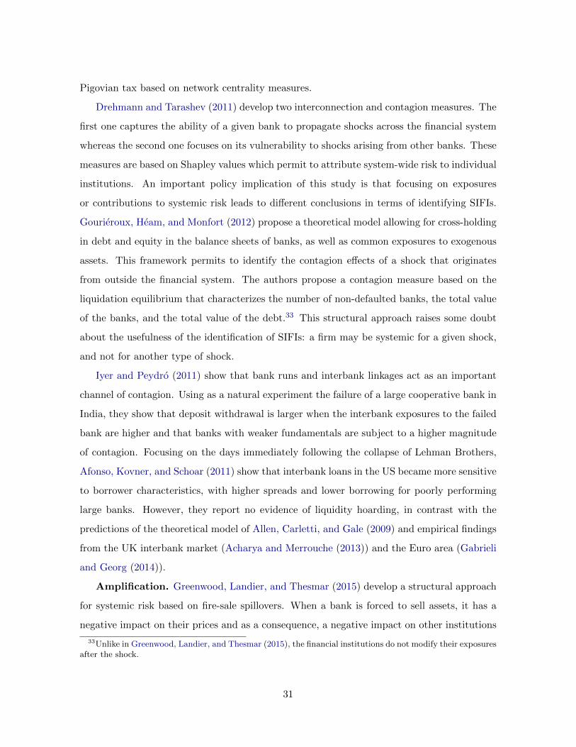
Pigovian tax based on network centrality measures.
Drehmann and Tarashev (2011) develop two interconnection and contagion measures. The
first one captures the ability of a given bank to propagate shocks across the financial system
whereas the second one focuses on its vulnerability to shocks arising from other banks. These
measures are based on Shapley values which permit to attribute system-wide risk to individual
institutions. An important policy implication of this study is that focusing on exposures
or contributions to systemic risk leads to different conclusions in terms of identifying SIFIs.
Gourieroux, Heam, and Monfort (2012) propose a theoretical model allowing for cross-holding
in debt and equity in the balance sheets of banks, as well as common exposures to exogenous
assets. This framework permits to identify the contagion effects of a shock that originates
from outside the financial system. The authors propose a contagion measure based on the
liquidation equilibrium that characterizes the number of non-defaulted banks, the total value
of the banks, and the total value of the debt.33 This structural approach raises some doubt
about the usefulness of the identification of SIFIs: a firm may be systemic for a given shock,
and not for another type of shock.
Iyer and Peydro (2011) show that bank runs and interbank linkages act as an important
channel of contagion. Using as a natural experiment the failure of a large cooperative bank in
India, they show that deposit withdrawal is larger when the interbank exposures to the failed
bank are higher and that banks with weaker fundamentals are subject to a higher magnitude
of contagion. Focusing on the days immediately following the collapse of Lehman Brothers,
Afonso, Kovner, and Schoar (2011) show that interbank loans in the US became more sensitive
to borrower characteristics, with higher spreads and lower borrowing for poorly performing
large banks. However, they report no evidence of liquidity hoarding, in contrast with the
predictions of the theoretical model of Allen, Carletti, and Gale (2009) and empirical findings
from the UK interbank market (Acharya and Merrouche (2013)) and the Euro area (Gabrieli
and Georg (2014)).
Amplification. Greenwood, Landier, and Thesmar (2015) develop a structural approach
for systemic risk based on fire-sale spillovers. When a bank is forced to sell assets, it has a
negative impact on their prices and as a consequence, a negative impact on other institutions
33Unlike in Greenwood, Landier, and Thesmar (2015), the financial institutions do not modify their exposuresafter the shock.
31

with similar exposures, hence the contagion. Their framework explains how the distribution
of leverage and risk exposures across banks contributes to systemic risk. It is based on the
key assumption that banks target a given level of leverage, which implies asset sales when
leverage is higher than the target. Bank vulnerability is defined as the impact on banks’ equity
of the deleveraging following a shock. The model is calibrated on European banks during the
2010-2011 sovereign debt crisis, as well as on US banks during the 2007-2009 financial crisis.
The authors show that microprudential interventions, which target the solvency of individual
banks, are always less effective than macroprudential policies which aim to minimize spillovers
across financial firms. Furthermore, the different measures perform well to capture the pre-
Lehman build-up in financial instability and the magnitude of the impact of Lehman’s failure
on the other banks. This result is confirmed by Duarte and Eisenbach (2015) who apply
similar systemic risk measures to a panel of US commercial banks and broker-dealers over a
longer time period. They show that the aggregate vulnerability measure starts increasing in
2004, long before many other systemic risk indicators, and reaches a peak in the fall of 2007.
In a related approach, Brunnermeier, Gorton, and Krishnamurthy (2014) present a liq-
uidity measure, called Liquidity Mismatch Index (LMI), which corresponds to the difference
between the “cash-equivalent” future values of the assets and of the liabilities of a bank. The
“cash-equivalent” value is defined as the product of the current value of the asset or liability,
multiplied by a liquidity weight (positive for assets, negative for liabilities) that depends on a
given stress scenario. Then, the Value-at-Liquidity-Risk is defined as the say 5% worst losses
and the Expected Liquidity Loss corresponds to the average of the liquidity losses beyond
this threshold. The authors propose to use LMI to identify the most systemically important
financial institutions. Jobst (2014) develops a structural model for liquidity risk that produces
estimates for both the probability and the severity of joint liquidity events, where the latter
are defined as situations in which banks jointly breach their NSFR ratios.
4.3 Global measures of systemic risk
A growing number of systemic risk measures are not targeted to a particular source of systemic
risk or a channel of transmission. Instead, they take a global, multi-channel approach to
systemic risk. The basic idea is that, if markets are efficient, a lot could be learned from
the current market prices of the securities issued by financial institutions, or from derivatives
32

written on them. Contrary to measures based on data disclosed with a lag (accounting data)
or on data not in the public domain (e.g. interconnectedness, substitutability), measures
based on market data can be freely computed in real time. As such, they may be better able
to detect sudden shifts in systemic risk regimes. However, a common pitfall of the measures
reviewed in this section is that they are rarely theoretically grounded and generally do not
permit to clearly identify the source of risk at play.
Four prominent examples of market-data based measures are the Marginal Expected Short-
fall (MES) and the Systemic Expected Shortfall (SES) of Acharya et al. (2010a), the Systemic
Risk Measure (SRISK) of Acharya, Engle, and Richardson (2012) and Brownlees and Engle
(2015), and the Delta Conditional Value-at-Risk (∆CoVaR) of Adrian and Brunnermeier
(2014). Over the past five years, hundreds of research articles have discussed, implemented,
and sometimes generalized, these systemic risk measures.34 As shown in Figure 1, these
systemic risk measures are the most central metrics in the systemic risk literature.
MES and SES. We consider N financial firms and denote rit the stock return of firm i
at time t. The market return is the value-weighted average of all individual returns, rmt =∑Ni=1witrit, where wit denotes the relative market capitalization of firm i. The MES is
the marginal contribution of an institution i to systemic risk, as measured by the Expected
Shortfall (ES) of the system. Originally proposed by Acharya et al. (2010a), the MES was
extended to a conditional version by Brownlees and Engle (2015). Formally, the conditional
ES of the system at time t is defined as:
ESmt (C) = Et−1(rmt | rmt < C) =
N∑i=1
witEt−1(rit | rmt < C), (6)
where C is a threshold. Then, the MES corresponds to the partial derivative of the system
ES with respect to the weight of firm i in the economy (Scaillet (2004)):
MESit (C) =∂ESmt (C)
∂wit= Et−1(rit | rmt < C). (7)
MES measures the increase in the risk of the system (measured by the ES) induced by a
marginal increase in the weight of firm i in the system. The SES extends the MES and
corresponds to the amount a bank’s equity drops below its target level (defined as a fraction
34As of November 2015, these papers have been collectively cited more than 2,700 times (Google Scholar).For online computation of some of these systemic risk measures, see the Stern-NYU’s V-Lab initiative athttp://vlab.stern.nyu.edu/welcome/risk/.
33

k of assets) in case of a systemic crisis when aggregate capital is less than k times aggregate
assets:SESitWit
= k Lit − 1− Et−1(rit |
∑N
i=1Wit < k
∑N
i=1Ait
), (8)
where Ait denotes the total assets, Wit the market capitalization or market value of equity,
and Lit the leverage, equal to Ait/Wit. Acharya et al. (2010a) show that the conditional
expectation term can be expressed as an increasing linear function of the MES:
SESit = (k Lit − 1 + θ MESit + ∆i) Wit, (9)
where θ and ∆i are constant terms.
SRISK. The SRISK measure proposed by Acharya, Engle, and Richardson (2012) and
Brownlees and Engle (2015) extends the MES in order to take into account both the liabilities
and the size of the financial institution. The SRISK corresponds to the expected capital
shortfall of a given financial institution, conditional on a crisis affecting the whole financial
system. In this perspective, the firms with the largest capital shortfall are assumed to be the
greatest contributors to the crisis and are the institutions considered the most systemically
risky. We follow Acharya, Engle, and Richardson (2012) and define the SRISK as:
SRISKit = max
0 ;
Required Capital︷ ︸︸ ︷k (Dit + (1− LRMESit)Wit)−
Available Capital︷ ︸︸ ︷(1− LRMESit)Wit
, (10)
where k is the prudential capital ratio, Dit the book value of total liabilities, and LRMES is
the long-run marginal expected shortfall, which corresponds to the expected drop in equity
value the firm would experiment if the market were to fall by more than a given threshold
within the next six months. As Lit = (Dit +Wit) /Wit, SRISK becomes:
SRISKit = max [0 ; [k Lit − 1 + (1− k) LRMESit]Wit] . (11)
We notice that SRISK increases with the leverage. Moreover, the expressions for SRISK and
SES in equations (9) and (11) are almost identical.
The SRISK considers the interconnections of a firm with the rest of the system through
the LRMES. Acharya, Engle, and Richardson (2012) propose to approximate it using the
daily MES (defined for a threshold C equal to 2%) as LRMESit ' 1 − exp (18×MESit).
34

This approximation represents the firm’s expected loss over a six-month horizon, obtained
conditionally on the market falling by more than 40% within the next six months.
∆CoVaR. Another popular systemic risk measure is the ∆CoVaR of Adrian and Brun-
nermeier (2014). CoV aRm|C(rit)it corresponds to the VaR of the market return obtained con-
ditionally on some event C (rit) observed for firm i:
Pr(rmt ≤ CoV aRm|C(rit)
it
∣∣∣ C (rit))
= α. (12)
The ∆CoVaR of firm i is then defined as the difference between the VaR of the financial
system conditional on this particular firm being in financial distress and the VaR of the
financial system conditional on firm i being in its median state. To define the distress of
a financial institution, various definitions of C (rit) can be considered. Because they use a
quantile regression approach, Adrian and Brunnermeier (2014) consider a situation in which
the loss is precisely equal to its VaR:
∆CoV aRit (α) = CoV aRm|rit=V aRit(α)it − CoV aRm|rit=Median(rit)
it . (13)
This definition is generalized by Girardi and Ergun (2013), who define the financial distress
of firm i as a situation in which the loss exceeds the VaR. We propose a comprehensive
comparison of these measures in Section 5, along with an empirical application.
Other global measures. Many other papers aim to extract information about systemic
risk from the joint distributions of banks’ extreme losses or returns. To our knowledge, the
first paper to introduce a measure of aggregate banking-system risk is Hartmann, Straetmans,
and de Vries (2007). Their tail-β captures the exposure of banks to extreme systematic shocks
and can be estimated using multivariate extreme value theory.
Billio et al. (2012) use quarterly returns on hedge funds, banks, broker-dealers, and
insurance companies to develop several measures of interconnectedness based on Granger
causality tests and principal component analysis (see also the absorption ratio of Kritzman et
al. (2011)). These measures provide direct estimates of the statistical connectivity within a
system of financial institutions, and show that banks have played a predominant role in trans-
mitting shocks compared to the other types of financial institutions. In the same vein, Diebold
and Yilmaz (2014) model stock returns in a vector autoregressive framework to empirically
estimate directional volatility connectedness measures among major US financial institutions.
35

Hautsch, Schaumburg, and Schienle (2015) define the systemic risk beta as the marginal effect
of a firm’s VaR on the system’s VaR. In order to capture network spillover effects, the VaR
of each firm is estimated by a quantile regression in which the set of regressors include other
firms’ extreme losses.
Another approach consists in estimating implied joint default probabilities for financial
institutions. Segoviano and Goodhart (2009) view the banking system as a portfolio of banks,
for which individual default probabilities can be estimated from structural approaches or se-
curities prices and, then aggregated at the system level using copulas. From the obtained
multivariate distribution of defaults, they derive several banking distress measures. Alter-
natively, Giglio (2014) uses bonds and Credit Default Swap (CDS) spreads to measure the
joint default of financial institutions. Huang, Zhou, and Zhu (2009) consider a hypothetical
portfolio that consists of the total liabilities of all banks and compute an expected portfolio
credit loss that exceeds a certain share of the banking sector’s total liabilities. This expected
loss also depends on banks’ CDS and corresponds to the actuarial premium of an insurance
policy that would protect against the distress of this portfolio, hence its name Distress In-
surance Premium (DIP). Oh and Patton (2015) compute a joint probability of distress based
on a dynamic copula model of CDS spreads. They show that idiosyncratic default risk has
been reduced since 2009 in the US whereas systemic risk increased during the post-crisis pe-
riod. Finally, Kelly, Lustig, and van Nieuwerburgh (2012) exploit option prices to show the
existence of a collective government guarantee for the US financial sector.
5 Systemic or systematic?
In this section, we derive new results on several prominent risk measures within a unified the-
oretical framework. This common framework allows to better understand their fundamental
differences, and in particular, the additional information that these systemic risk metrics are
able to provide over and above systematic market risk measures such as beta or correlation.
5.1 Common theoretical framework
Consider a bivariate GARCH process for the vector of market and firm demeaned returns
r′t = (rmt rit), such that:
rt = H1/2t νt, (14)
36

where the innovation ν ′t = (εmt ξit) is i.i.d. with E (νt) = 0 and E (νtν′t) = I2, a two-by-two
identity matrix, and the conditional variance-covariance matrix Ht is defined as:
Ht =
(σ2mt σit σmt ρit
σit σmt ρit σ2it
), (15)
where σit and σmt denote the conditional standard deviations and ρit the conditional correla-
tion. For simplicity, we assume that the innovations εmt and ξit are independently distributed
at time t, which means that the time-varying conditional correlation ρit fully captures the
dependence between the firm and market returns.35
Under these assumptions, we can show that the MES of a given financial institution i is
proportional to its systematic risk, as measured by its time-varying beta. The proportionality
coefficient is the expected shortfall of the market:
MESit (α) = βit ESmt (α) , (16)
where ESmt (α) = Et−1 (rmt | rmt < V aRmt(α)) is the expected shortfall of the market and
βit = ρitσit/σmt the time-varying beta of firm i. The proof of Equation (16) is in Benoit
et al. (2013) (Appendix A) and in Brownlees and Engle (2015). This result has two main
implications. First, on a given date, the systemic risk ranking of financial institutions based on
MES is strictly equivalent to the ranking that would be produced by sorting them according to
their betas. Indeed, since the system expected shortfall is not firm-specific, a firm’s estimated
systemic importance simply increases with its market beta. Second, for a given financial
institution, the time profile of its systemic risk measured by its MES may be different from
the evolution of its systematic risk measured by its conditional beta. Since the market ES
may not be constant over time, forecasting the systematic risk of firm i may not be sufficient
to forecast the future evolution of its contribution to systemic risk.
As SRISK is a function of the MES, SRISK can be expressed as a function of the beta,
leverage, and market capitalization of the financial institution:
SRISKit ' max [0 ; [k(Lit − 1) + (1− k) exp (18× βit × ESmt (α))]Wit] . (17)
SRISK is an increasing function of the systematic risk, as measured by the conditional beta
since ESmt (α) is typically a negative number and the prudential capital ratio k is smaller than
35We will relax this assumption in the empirical analysis in Section 5.2.
37

one. However, unlike with MES, systemic-risk rankings based on SRISK are not equivalent
to rankings based on betas. SRISK-based rankings also depend on the leverage and on the
market capitalization of the financial institution. Accounting for market capitalization and
liabilities in the definition of the systemic risk measure tends to increase the systemic risk score
of large firms. This result is in line with the too-big-to-fail paradigm, whereas the MES tends
to be naturally driven by interconnected institutions (through the beta), which is more in line
with the too-interconnected-to-fail paradigm (Markose, Giansante, and Shaghaghi (2012)). In
that sense, the SRISK can be viewed as a compromise between both paradigms.36
Within this framework, it is also possible to express ∆CoVaR, defined for the conditioning
event rit = V aRit (α), as a function of the conditional correlations, volatilities, and VaR.
Given Equations (14) and (15), we can show that the ∆CoVaR of a given financial institution
i is proportional to its tail risk, as measured by its VaR. The proportionality coefficient
corresponds to the linear projection coefficient of the market return on the firm return.
∆CoV aRit (α) = γit [V aRit (α)− V aRit (0.5)] , (18)
where γit = ρitσmt/σit. If the marginal distribution of the return is symmetric around zero,
∆CoVaR is:
∆CoV aRit (α) = γit V aRit (α) . (19)
The proof of Equation (19) is in Benoit et al. (2013) (Appendix B).37 The fact that the
proportionality coefficient between ∆CoVaR and VaR is firm-specific implies that the most
risky institutions (in terms of VaR) are not necessarily the most systemically risky ones (in
terms of ∆CoVaR). In that sense, ∆CoVaR is not equivalent to VaR in the cross-section, as
already pointed out by Adrian and Brunnermeier (2014) in their Figure 1. However, for a given
institution i, when the variance-covariance matrix is constant or when ∆CoVaR is estimated
by quantile regression as in Adrian and Brunnermeier (2014), the coefficient γit is constant over
time. In that case, ∆CoVaR becomes proportional to VaR and, as a consequence, forecasting
the systemic contribution of a firm is equivalent to forecasting its tail risk in isolation.
36Engle, Jondeau, and Rockinger (2015) use SRISK divided by the GDP of a country to sort domestic banksand identify domestic systemically important banks.
37Under the normality assumption, Adrian and Brunnermeier (2014) also show that ∆CoVaR is a functionof VaR: ∆CoV aRit (α) = ρitσmtΦ
−1 (α) or equivalently γitσitΦ−1 (α), where σitΦ
−1 (α) denotes the VaR(α)of the firm.
38

5.2 Empirical illustration
The theoretical results derived in Section 5.1 have been derived within a specific common
framework. However, in practice, the dependence between financial asset returns may be
richer (i.e., not linear) and thus our results may not hold in real financial markets. For this
reason, we now relax the assumptions made in Equations (14) and (15) for asset returns. In
our empirical analysis, we implement the same estimation methods as in the original articles
presenting the MES, SRISK, and ∆CoVaR, and we use the same sample as in Acharya,
Pedersen, Philippon, and Richardson (2010a). This sample contains all US financial firms
with a market capitalization greater than $5 billion as of end of June 2007. For our sample
period, January 3, 2000 - December 31, 2010, we extract daily firm stock returns, value-
weighted market index returns, number of shares outstanding, and daily closing prices from
CRSP. Quarterly book values of total liabilities are from COMPUSTAT. Following Brownlees
and Engle (2015), we estimate the MES and SRISK using a GARCH-DCC model. We use a
coefficient α of 5%, and the threshold C is set equal to the unconditional market daily VaR
at 5%, which is equal to 2.52% in our sample. The ∆CoVaR is estimated with a quantile
regression as proposed by Adrian and Brunnermeier (2014).
We first investigate the relationship between MES and beta in Figure 3. This scatter
plot compares the average MES, MESi (α) = T−1∑T
t=1 |MESit (α)|, to the average beta,
βi = T−1∑T
t=1 βit, for the 61 firms that have been continuously traded during our sample
period. This plot confirms the strong relationship between MES (y-axis) and firm beta (x-
axis). In line with Equation (16), the OLS estimated slope coefficient (0.0248) is extremely
close to the unconditional ES of the market at 5%, 0.0252 or 2.52%.38 The main implication
of this result is that systemic risk rankings of financial institutions based on their MES tend
to mirror rankings obtained by sorting firms on betas.
Should one worry about the fact that MES and beta give similar rankings? We think that
this is a serious concern for the following reasons. First, if beta is believed to be a good proxy
for systemic risk, why not rank firms on betas in the first place? Second, this leads to confusion
between systemic risk and systematic risk (market risk); the latter being already accounted
for in the banking regulation since the 1996 Amendment of the Basel Accord as regulatory
38Similar results (not reported) are obtained when we consider constant betas rather than conditional betas,or when we consider the firm’s MES and beta at a given point in time rather than averages.
39
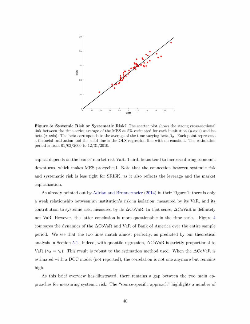
0 0.2 0.4 0.6 0.8 1 1.2 1.4 1.6 1.8 20
0.01
0.02
0.03
0.04
0.05
Beta
ME
S
Figure 3: Systemic Risk or Systematic Risk? The scatter plot shows the strong cross-sectionallink between the time-series average of the MES at 5% estimated for each institution (y-axis) and itsbeta (x-axis). The beta corresponds to the average of the time-varying beta βit. Each point representsa financial institution and the solid line is the OLS regression line with no constant. The estimationperiod is from 01/03/2000 to 12/31/2010.
capital depends on the banks’ market risk VaR. Third, betas tend to increase during economic
downturns, which makes MES procyclical. Note that the connection between systemic risk
and systematic risk is less tight for SRISK, as it also reflects the leverage and the market
capitalization.
As already pointed out by Adrian and Brunnermeier (2014) in their Figure 1, there is only
a weak relationship between an institution’s risk in isolation, measured by its VaR, and its
contribution to systemic risk, measured by its ∆CoVaR. In that sense, ∆CoVaR is definitely
not VaR. However, the latter conclusion is more questionable in the time series. Figure 4
compares the dynamics of the ∆CoVaR and VaR of Bank of America over the entire sample
period. We see that the two lines match almost perfectly, as predicted by our theoretical
analysis in Section 5.1. Indeed, with quantile regression, ∆CoVaR is strictly proportional to
VaR (γit = γi). This result is robust to the estimation method used. When the ∆CoVaR is
estimated with a DCC model (not reported), the correlation is not one anymore but remains
high.
As this brief overview has illustrated, there remains a gap between the two main ap-
proaches for measuring systemic risk. The “source-specific approach” highlights a number of
40

Jan00 Mar02 May04 Aug06 Oct08 Dec100
0.02
0.04
0.06BAC
∆Co
VaR
0
0.1
0.2
0.3
VaR
∆CoVaRVaR
Figure 4: CoVaR is Equivalent to VaR in Time Series. The figure displays the ∆CoVaR (solidline, left y-axis) and the 5%-VaR (dashed line, right y-axis) of Bank of America (BAC).
mechanisms, which lead to a host of different risk measures and regulations. Despite many
appealing properties, even the best global measures cannot encompass this variety of systemic
risk sources. Indeed, a limited number of variables seem sufficient to capture their variation
in the cross section (MES and SRISK) or in the time series dimension (∆CoVaR). Regulatory
authorities, with their preferred access to proprietary data, keep using their own approach to
produce global measures of systemic risk, with the shortcomings pointed out in Section 4.1.
6 Validation
As we have seen in the previous two sections, there is an impressive variety of competing
systemic risk measures. Regulators and other end-users of these measures thus need guidance
on how to select the ones most adapted to their objectives. To this end, we compared some of
the most popular measures in Section 5. We review in this section other recent attempts to
contrast existing measures, following two approaches: an ex ante comparison of risk measures
based on their mathematical properties, and an ex post approach based on their empirical
performance.
41

6.1 Theoretical analysis of risk measures
As of yet, only few papers analyze the desirable properties that a sound systemic risk measure
should comply with. Following the coherent risk approach of Artzner et al. (1999), Chen,
Iyengar, and Moallemi (2013) define an axiomatic framework for systemic risk measures. Their
analysis is based on the joint distribution of outcomes across all financial firms and all states
of nature. In this framework, a systemic risk measure is a function from the space of firms and
outcomes to R. This function must satisfy the main conditions that define any coherent risk
measure, namely the monotonicity, positive homogeneity, and outcome convexity axioms.39
However, a systemic risk measure must also satisfy an additional preference consistency axiom.
This axiom states that the risk measure has to reflect the preference of the regulator on the
cross-sectional profile of losses across firms and the distribution of the aggregate outcomes
across states. Brunnermeier and Oehmke (2013a) also require a measure to satisfy the clone
property: if a financial institution is split into several equal parts, the total systemic risk does
not change, since risk is also equally divided. When complying with this property, a measure
captures systemic risk originating from small institutions that behave in a correlated way.
A good risk measure should also allow regulators to impose a firm-specific capital sur-
charge in an economically consistent way. Gourieroux and Monfort (2013) propose a set of
axioms (decentralization, additivity, and risk ordering) for dividing an aggregate systemic risk
measure into individual contributions. In particular, they show that the Shapley value does
not satisfy these axioms, while the Euler equation does. Brunnermeier and Cheridito (2014)
introduce SystRisk which is a measure of total systemic risk satisfying the allocation and clone
properties. Furthermore, their measure includes a tolerance parameter that can be adjusted
over time to implement countercyclical regulation, especially when volatility is low.
These different approaches assume that the risk measure is correctly estimated. Given the
variety of risk measures that have been proposed and data limitations, any single systemic risk
measure will necessarily be fraught with uncertainty. Hansen (2013) discusses the challenge
of measuring this uncertainty and designing regulatory approaches that are robust to this
problem.
39The monotonicity condition reflects that if one firm has greater losses in every scenario than another, it isless preferred. The positive homogeneity implies that the risk measure increases in proportion to the scale oflosses. The outcome convexity condition is the basis of the diversification principle: the risk of a firm diversifiedbetween two outcomes is lower than the weighted risk that corresponds to these two outcomes.
42

6.2 Empirical assessment of risk measures
Empirical validation is a key requirement for any systemic risk measure to become an industry
standard. There is no consensus at the moment, and several approaches have been followed
in the academic literature. Brownlees and Engle (2015) show that banks with higher SRISK
before the financial crisis were more likely to be bailed out by the government and to receive
capital injections from the Federal Reserve. Alternative approaches include testing whether
firms with high systemic risk scores are more likely to become insolvent (Wu and Zhao (2014)),
to suffer the highest financial losses (Idier, Lame, and Mesonnier (2014)), or to have the most
negative stock returns (Acharya, Engle, and Richardson (2012)) in a financial crisis.
For firm-level measures, one can compare the empirical ranking obtained with a given
measure with the one computed by the FSB, which is based on confidential bank supervisory
data (Engle, Jondeau, and Rockinger (2015)). Cai, Saunders, and Steffen (2014) find a
positive correlation between interconnectedness (measured by being member of the same loan
syndicate) and standard bank-level systemic risk measures including SRISK, CoVaR, and
DIP, during recessions. Another strategy followed by Duarte and Eisenbach (2015) is to show
that their risk measure Granger-causes most other systemic risk measures. In the same vein,
Rodrıguez-Moreno and Pena (2013) compare several market-based systemic risk measure and
rank these measures using three criteria to argue that systemic risk measures based on CDSs
outperform measures based on interbank interest rates or stock market prices.
For systemic risk measures defined at the system level, one can test whether a high sys-
temic risk score can be seen as an early warning signal and is positively and significantly
associated with future systemic risk events. Allen, Bali, and Tang (2012) show that high
levels of systemic risk in the banking sector, as captured by their CATFIN measure, impact
the macroeconomy through aggregate lending activity. They show that CATFIN can forecast
macroeconomic downturns approximately six months before they occur. Similarly, Giglio,
Kelly, and Pruitt (2015) test whether existing systemic risk measures are able to predict
macroeconomic downturns using long times series (starting in the 1920’s) and international
data.
43

7 Conclusion
Despite the breathtaking pace at which research on systemic risk has progressed, much remains
to be done. This survey can serve as a catalyst for future developments in at least three areas
which we list below.
Measurement is a key issue for policymakers, who are looking for tools to monitor the
building up of risks and quantify the negative externalities imposed by systemic institutions
on the whole system. Many methodologies are now available to identify different sources of
systemic risk and will probably be developed into full fledged regulatory tools in the near
future. What is less clear is how to link the measures produced by these tools to regulatory
interventions: observing that a bank has become more central in the interbank market does not
translate directly into a clear policy response. More structural models, linking risk estimates
to well-defined policy objectives and available tools, would be useful to regulators.
The economic mechanisms leading to systemic risk have been researched for even longer,
so that we now have a good understanding of where the risks can lie. However, the issue of
how to optimally regulate banks and correct the different market failures leading to systemic
risk has been less investigated. In particular, many macroprudential tools are quite new and
the extent of their impact is not fully understood yet, neither theoretically nor empirically.
There will be an important learning-by-doing process as regulators will increasingly make use
of the new toolbox, giving empiricists experiments to analyze and theorists stylized facts to
explain.
The quest for a global risk measure that encompasses different sources of systemic risk,
and yet produces a single metric that can directly be used for regulation, is still ongoing.
However, we have reasons to remain optimistic as more data are becoming available, with
better quality, higher frequency, and wider scope (see the G20 Data Gaps Initiative, Cerutti,
Claessens, and McGuire (2014)). Given the very nature of systemic risk, future risk measures
should combine various sources of information, including balance-sheet data, proprietary data
on positions, and market data, as well as regulators’ assessments of banks’ interconnectedness
and riskiness. In the future, such an approach could complement or eventually replace a host
of technical macroprudential tools by a simple systemic risk tax or capital surcharge aligning
systemic banks’ interests with the social optimum. This would have significant benefits in
44

terms of efficiency and simplicity.
45

References
Acemoglu, D., A. Ozdaglar, and A. Tahbaz-Salehi (2015): “Systemic Risk and Stability in
Financial Networks,” The American Economic Review, 105(2), 564–608. 14, 30
Acharya, V. V. (2001): “A Theory of Systemic Risk and Design of Prudential Bank Regulation,
Unabridged version,” Working paper. 2, 3, 29
(2003): “Is the International Convergence of Capital Adequacy Regulation Desirable?,” The
Journal of Finance, 58(6), 2745–2782. 24
(2009): “A theory of systemic risk and design of prudential bank regulation,” Journal of
Financial Stability, 5(3), 224–255. 9
Acharya, V. V., and A. Bisin (2014): “Counterparty risk externality: Centralized versus over-the-
counter markets,” Journal of Economic Theory, 149(C), 153–182. 15
Acharya, V. V., T. Cooley, M. Richardson, and I. Walter (2010): “Manufacturing Tail Risk:
A Perspective on the Financial Crisis of 2007-2009,” Foundations and Trends in Finance, 4(4),
247–325. 11
Acharya, V. V., R. Engle, and M. Richardson (2012): “Capital Shortfall: A New Approach to
Ranking and Regulating Systemic Risks,” The American Economic Review, 102(3), 59–64. 33, 34,
43
Acharya, V. V., D. Gale, and T. Yorulmazer (2011): “Rollover Risk and Market Freezes,” The
Journal of Finance, 66(4), 1177–1209. 17
Acharya, V. V., and O. Merrouche (2013): “Precautionary Hoarding of Liquidity and Interbank
Markets: Evidence from the Subprime Crisis,” Review of Finance, 17(1), 107–160. 3, 31
Acharya, V. V., and H. Naqvi (2012): “The seeds of a crisis: A theory of bank liquidity and risk
taking over the business cycle,” Journal of Financial Economics, 106(2), 349–366. 13
Acharya, V. V., and T. Oncu (2013): “A Proposal for the Resolution of Systemically Important
Assets and Liabilities: The Case of the Repo Market,” International Journal of Central Banking,
9(s1), 291–349. 21
Acharya, V. V., L. H. Pedersen, T. Philippon, and M. Richardson (2010a): “Measuring
systemic risk,” Working paper. 3, 9, 39
Acharya, V. V., L. H. Pedersen, T. Philippon, and M. Richardson (2010b): “Taxing Systemic
Risk,” in Regulating Wall Street: The Dodd-Frank Act and the New Architecture of Global Finance,
ed. by V. Acharya, T. Cooley, M. Richardson, and Walter, pp. 121–142. Princeton University Press.
27, 33, 34
Acharya, V. V., and A. Thakor (2015): “The dark side of liquidity creation: leverage and systemic
risk,” Working paper. 15
46

Acharya, V. V., and T. Yorulmazer (2008a): “Cash-in-the-Market Pricing and Optimal Resolu-
tion of Bank Failures,” Review of Financial Studies, 21(6), 2705–2742. 10
(2008b): “Information Contagion and Bank Herding,” Journal of Money, Credit and Banking,
40(1), 215–231. 10
Adrian, T., and M. Brunnermeier (2014): “CoVaR,” Working paper. 3, 33, 35, 38, 39, 40
Adrian, T., and H. S. Shin (2014): “Procyclical Leverage and Value-at-Risk,” Review of Financial
Studies, 27(2), 373–403. 12
Afonso, G., A. Kovner, and A. Schoar (2011): “Stressed, Not Frozen: The Federal Funds Market
in the Financial Crisis,” The Journal of Finance, 66(4), 1109–1139. 3, 31
Afonso, G., and H. S. Shin (2011): “Precautionary Demand and Liquidity in Payment Systems,”
Journal of Money, Credit & Banking, 43(7), 589–619. 15
Agarwal, S., D. Lucca, A. Seru, and F. Trebbi (2014): “Inconsistent Regulators: Evidence
from Banking,” Quarterly Journal of Economics, 129(2), 889–938. 25
Aghion, P., P. Bolton, and M. Dewatripont (2000): “Contagious bank failures in a free banking
system,” European Economic Review, 44(4-6), 713–718. 15
Aiyar, S., C. W. Calomiris, and T. Wieladek (2014): “Does Macro-Prudential Regulation Leak?
Evidence from a UK Policy Experiment,” Journal of Money, Credit and Banking, 46(s1), 181–214.
3, 20
Allen, F., and A. Babus (2009): “Networks in Finance,” in Network-based Strategies and Compe-
tencies, ed. by P. Kleindorfer, and J. Wind, pp. 367–382. Wharton School Publishing. 14
Allen, F., A. Babus, and E. Carletti (2012): “Asset commonality, debt maturity and systemic
risk,” Journal of Financial Economics, 104(3), 519–534. 14
Allen, F., and E. Carletti (2013): “Systemic risk from real estate and macro-prudential regula-
tion,” International Journal of Banking, Accounting and Finance, 5(1/2), 28–48. 13
Allen, F., E. Carletti, and D. Gale (2009): “Interbank market liquidity and central bank
intervention,” Journal of Monetary Economics, 56(5), 639–652. 31
Allen, F., E. Carletti, I. Goldstein, and A. Leonello (2015): “Government guarantees and
financial stability,” CEPR Discussion Paper Series 10560. 22
Allen, F., and D. Gale (1994): “Limited Market Participation and Volatility of Asset Prices,” The
American Economic Review, 84(4), 933–955. 16
(2000a): “Bubbles and Crises,” The Economic Journal, 110(460), 236–255. 13
(2000b): “Financial Contagion,” Journal of Political Economy, 108(1), 1–33. 2, 3, 13
(2004a): “Financial Fragility, Liquidity, and Asset Prices,” Journal of the European Economic
Association, 2(6), 1015–1048. 16
47

(2004b): “Financial Intermediaries and Markets,” Econometrica, 72(4), 1023–1061. 16
(2007): “Systemic Risk and Regulation,” in The Risks of Financial Institutions, NBER
Chapters, pp. 341–376. National Bureau of Economic Research. 21
Allen, L., T. G. Bali, and Y. Tang (2012): “Does Systemic Risk in the Financial Sector Predict
Future Economic Downturns?,” Review of Financial Studies, 25(10), 3000–3036. 43
Allen, W. A., and R. Moessner (2010): “Central bank co-operation and international liquidity in
the financial crisis of 2008-9,” Working Paper 310, Bank for International Settlements. 11
Alter, A., B. R. Craig, and P. Raupach (2015): “Centrality-Based Capital Allocations,” Inter-
national Journal of Central Banking, 11(3), 329–377. 21
Anand, K., P. Gai, S. Kapadia, S. Brennan, and M. Willison (2013): “A network model of
financial system resilience,” Journal of Economic Behavior & Organization, 85(C), 219–235. 14
Arora, S., B. Barak, M. Brunnermeier, and R. Ge (2009): “Computational Complexity and
Information Asymmetry in Financial Products,” Working paper. 18
Artzner, P., F. Delbaen, J.-M. Eber, and D. Heath (1999): “Coherent measures of risk,”
Mathematical Finance, 9(3), 203–228. 42
Babus, A. (2015): “The Formation of Financial Networks,” RAND Journal of Economics, Forthcom-
ing. 14
Babus, A., and T.-W. Hu (2015): “Endogenous Intermediation in Over-the-Counter Markets,”
Working paper, Federal Reserve Bank of Chicago. 14
Babus, A., and P. Kondor (2013): “Trading and Information Diffusion in Over-the-Counter Mar-
kets,” Working paper, Federal Reserve Bank of Chicago. 14
Bae, K.-H., G. A. Karolyi, and R. M. Stulz (2003): “A New Approach to Measuring Financial
Contagion,” Review of Financial Studies, 16(3), 717–763. 3, 16
Banerjee, R. N., and H. Mio (2014): “The Impact of Liquidity Regulation on Banks,” BIS Working
Papers 470, Bank for International Settlements. 3
Basel Committee on Banking Supervision (1991): “Measuring and controlling large credit ex-
posures,” Report. 21
(2011): “Basel III: A Global Framework for more Resilient Banks and Banking Systems,”
Report. 19
(2013a): “Basel III: The Liquidity Coverage Ratio and Liquidity Risk Monitoring Tools,”
Report. 20
(2013b): “Global Systemically Important Banks: Updated Assessment Methodology and the
Higher Loss Absorbency Requirement,” Report. 24, 28
48

(2014a): “Basel III: Leverage Ratio Framework and Disclosure Requirements,” Report. 19
(2014b): “Basel III: The Net Stable Funding Ratio,” Report. 20
(2014c): “Supervisory framework for measuring and controlling large exposures - final stan-
dard,” Report. 21
Basel Committee on Banking Supervision and Board of the International organization
of Securities Commissions (2013): “Margin Requirements for non-centrally cleared derivatives,”
Report. 22
Benoit, S., G. Colletaz, C. Hurlin, and C. Perignon (2013): “A Theoretical and Empirical
Comparison of Systemic Risk Measures,” Working paper. 37, 38
Benoit, S., C. Hurlin, and C. Perignon (2015): “Implied Risk Exposures,” Review of Finance,
Forthcoming. 12
Bernanke, B., and M. Gertler (1989): “Agency Costs, Net Worth, and Business Fluctuations,”
The American Economic Review, 79(1), 14–31. 2, 3, 12
Bernanke, B. S. (2013): “Stress Testing Banks: What Have We Learned?,” Remarks by Chairman
Ben S. Bernanke at the ”Maintaining Financial Stability: Holding a Tiger by the Tail” Federal
Reserve Bank of Atlanta conference. 21
Bernardo, A. E., and I. Welch (2004): “Liquidity and Financial Market Runs,” The Quarterly
Journal of Economics, 119(1), 135–158. 18
Bhattacharya, S., and D. Gale (1987): “Preference shocks, liquidity and central bank policy,” in
New Approaches to Monetary Economics, ed. by W. Barnett, and K. Singleton, pp. 69–88. Cam-
bridge University Press. 3, 11
Bhattacharya, S., C. Goodhart, D. Tsomocos, and A. Vardoulakis (2011): “Minsky’s Fi-
nancial Instability Hypothesis and the Leverage Cycle,” Working paper. 12
Biais, B., F. Heider, and M. Hoerova (2015): “Risk-sharing or risk-taking? An incentive theory
of counterparty risk, clearing and margins,” The Journal of Finance, Forthcoming. 15
Biais, B., T. Mariotti, J.-C. Rochet, and S. Villeneuve (2010): “Large Risks, Limited Lia-
bility, and Dynamic Moral Hazard,” Econometrica, 78(1), 73–118. 12
Bianchi, J., and E. G. Mendoza (2015): “Optimal Time-Consistent Macroprudential Policy,”
Working Paper 19704, National Bureau of Economic Research. 20
Billio, M., M. Getmansky, A. W. Lo, and L. Pelizzon (2012): “Econometric measures of con-
nectedness and systemic risk in the finance and insurance sectors,” Journal of Financial Economics,
104(3), 535–559. 3, 35
Bisias, D., M. Flood, A. W. Lo, and S. Valavanis (2012): “A Survey of Systemic Risk Analytics,”
Annual Review of Financial Economics, 4(1), 255–296. 7
49

Blei, S., and B. Ergashev (2014): “Asset commonality and systemic risk among large banks in the
United States,” Working paper. 3, 29
Boissay, F., F. Collard, and F. Smets (2015): “Booms and systemic banking crises,” Journal of
Political Economy, Forthcoming. 12
Borio, C. (2003): “Towards a macroprudential framework for financial supervision and regulation?,”
Working Paper 128, Bank for International Settlements. 2
Boss, M., H. Elsinger, M. Summer, and S. Thurner (2004): “Network topology of the interbank
market,” Quantitative Finance, 4(6), 677–684. 14
Bouvard, M., P. Chaigneau, and A. De Motta (2015): “Transparency in the Financial System:
Rollover Risk and Crises,” The Journal of Finance, 70(4), 1805–1837. 23
Boyson, N. M., C. W. Stahel, and R. M. Stulz (2010): “Hedge Fund Contagion and Liquidity
Shocks,” The Journal of Finance, 65(5), 1789–1816. 17
Brownlees, T. C., and R. F. Engle (2015): “SRISK: A conditional capital shortfall index for
systemic risk measurement,” Working paper. 3, 33, 34, 37, 39, 43
Brunnermeier, M., G. Gorton, and A. Krishnamurthy (2014): “Liquidity Mismatch Mea-
surement,” in Risk Topography: Systemic Risk and Macro Modeling, NBER Chapters, pp. 99–112.
National Bureau of Economic Research. 3, 32
Brunnermeier, M. K., and P. Cheridito (2014): “Measuring and allocating systemic risk,” Work-
ing paper. 42
Brunnermeier, M. K., T. M. Eisenbach, and Y. Sannikov (2013): “Macroeconomics with
Financial Frictions: A Survey,” in Advances in Economics and Econometrics, Tenth World Congress
of the Econometric Society, Vol. 2, pp. 3–96. Cambridge University Press, New York. 12
Brunnermeier, M. K., and M. Oehmke (2013a): “Bubbles, financial crises, and systemic risk,” in
Handbook of the Economics of Finance, ed. by M. H. George M. Constantinides, and R. M. Stulz,
pp. 1221–1288. Elsevier. 13, 42
Brunnermeier, M. K., and M. Oehmke (2013b): “The Maturity Rat Race,” The Journal of
Finance, 68(2), 483–521. 3, 11, 18
Brunnermeier, M. K., and L. H. Pedersen (2009): “Market Liquidity and Funding Liquidity,”
Review of Financial Studies, 22(6), 2201–2238. 3, 16, 17
Brunnermeier, M. K., and Y. Sannikov (2014): “A Macroeconomic Model with a Financial
Sector,” The American Economic Review, 104(2), 379–421. 12
Bryant, J. (1980): “A model of reserves, bank runs, and deposit insurance,” Journal of Banking &
Finance, 4(4), 335–344. 18
Caballero, R., and A. Simsek (2013): “Fire Sales in a Model of Complexity,” The Journal of
Finance, 68(6), 2549–2587. 18
50

Cai, J., A. Saunders, and S. Steffen (2014): “Syndication, interconnectedness and systemic risk,”
Working paper. 29, 43
Calomiris, C. W., and C. M. Kahn (1991): “The Role of Demandable Debt in Structuring Optimal
Banking Arrangements,” The American Economic Review, 81(3), 497–513. 3, 18
Calomiris, C. W., and J. R. Mason (1997): “Contagion and Bank Failures during the Great
Depression: The June 1932 Chicago Banking Panic,” The American Economic Review, 87(5), 863–
883. 3, 16
Castiglionesi, F., and N. Navarro (2011): “Fragile Financial Networks,” Working paper. 14
Cerutti, E., S. Claessens, and P. McGuire (2014): “Systemic risks in global banking: what can
available data tell us and what more data are needed?,” in Risk Topography: Systemic Risk and
Macro Modeling, NBER Chapters, pp. 235–260. National Bureau of Economic Research. 44
Cespa, G., and T. Foucault (2014): “Illiquidity Contagion and Liquidity Crashes,” Review of
Financial Studies, 27(6), 1615–1660. 16
Chan, N., M. Getmansky, S. M. Haas, and A. W. Lo (2007): “Systemic Risk and Hedge Funds,”
in The Risks of Financial Institutions, NBER Chapters, pp. 235–338. National Bureau of Economic
Research. 11
Chen, C., G. Iyengar, and C. C. Moallemi (2013): “An Axiomatic Approach to Systemic Risk,”
Management Science, 59(6), 1373–1388. 42
Chen, Q., I. Goldstein, and W. Jiang (2010): “Payoff complementarities and financial fragility:
Evidence from mutual fund outflows,” Journal of Financial Economics, 97(2), 239–262. 3, 18
Chen, Y. (1999): “Banking Panics: The Role of the First-Come, First-Served Rule and Information
Externalities,” Journal of Political Economy, 107(5), 946–968. 3, 15
Cifuentes, R., H. S. Shin, and G. Ferrucci (2005): “Liquidity Risk and Contagion,” Journal of
the European Economic Association, 3(2-3), 556–566. 17
Claessens, S. (2014): “An Overview of Macroprudential Policy Tools,” Working Paper 14/214,
International Monetary Fund. 19
Clerc, L., A. Derviz, C. Mendicino, S. Moyen, K. Nikolov, L. Stracca, J. Suarez, and
A. P. Vardoulakis (2015): “Capital Regulation in a Macroeconomic Model with Three Layers of
Default,” International Journal of Central Banking, 11(3), 9–63. 21
Coval, J., and E. Stafford (2007): “Asset fire sales (and purchases) in equity markets,” Journal
of Financial Economics, 86(2), 479–512. 16
Crockett, A. (2000): “Marrying the micro- and macroprudential dimensions of financial stability,”
BIS Speeches. 2
Crowe, C., G. Dell’Ariccia, D. Igan, and P. Rabanal (2013): “How to deal with real estate
booms: Lessons from country experiences,” Journal of Financial Stability, 9(3), 300–319. 19
51
Danıelsson, J. (2008): “Blame the models,” Journal of Financial Stability, 4(4), 321–328. 21
Danıelsson, J., H. S. Shin, and J.-P. Zigrand (2004): “The impact of risk regulation on price
dynamics,” Journal of Banking & Finance, 28(5), 1069–1087. 12
Dasgupta, A. (2004): “Financial Contagion Through Capital Connections: A Model of the Origins
and Spread of Bank Panics,” Journal of the European Economic Association, 2(6), 1049–1084. 3, 16
De Bandt, O., and P. Hartmann (2002): “Systemic Risk: A Survey,” in Financial Crisis, Con-
tagion and the Lender of Last Resort: A Book of Readings, ed. by C. Goodhart, and G. Illing, pp.
249–298. Oxford University Press, Oxford. 7
De Bandt, O., P. Hartmann, and J.-L. Peydro (2012): “Systemic Risk in Banking: An Update,”
in The Oxford Handbook of Banking, ed. by A. N. Berger, P. Molyneux, and J. Wilson, pp. 633–672.
Oxford University Press. 7
De Nicolo, G., A. Gamba, and M. Lucchetta (2014): “Microprudential Regulation in a Dynamic
Model of Banking,” Review of Financial Studies, 27(7), 2097–2138. 26
De Nicolo, G., and M. Lucchetta (2011): “Systemic Risks and the Macroeconomy,” in Quan-
tifying Systemic Risk, NBER Chapters, pp. 113–148. National Bureau of Economic Research. 3,
30
Dell’Ariccia, G., and R. Marquez (2006): “Competition among regulators and credit market
integration,” Journal of Financial Economics, 79(2), 401–430. 24
Diamond, D. W., and P. H. Dybvig (1983): “Bank Runs, Deposit Insurance, and Liquidity,”
Journal of Political Economy, 91(3), 401–419. 3, 18
Diamond, D. W., and R. G. Rajan (2005): “Liquidity Shortages and Banking Crises,” The Journal
of Finance, 60(2), 615–647. 17
Diebold, F. X., and K. Yilmaz (2014): “On the network topology of variance decompositions:
Measuring the connectedness of financial firms,” Journal of Econometrics, 182(1), 119–134. 35
Drehmann, M., and N. Tarashev (2011): “Systemic importance: Some simple indicators,” BIS
Quarterly Review. 3, 31
Duarte, F., and T. Eisenbach (2015): “Fire-sale spillovers and systemic risk,” Staff Reports 645,
Federal Reserve Bank of New York. 3, 32, 43
Duffie, D. (2010): “The Failure Mechanics of Dealer Banks,” The Journal of Economic Perspectives,
24(1), 51–72. 18
(2013): “Replumbing Our Financial System: Uneven Progress,” International Journal of
Central Banking, 9(S1), 251–279. 22
(2014): “Financial Market Infrastructure: Too Important to Fail,” in Across the Great Divide:
New Perspectives on the Financial Crisis, ed. by M. N. Baily, and J. B. Taylor, Book Chapters,
chap. 11, pp. 251–257. Hoover Institution, Stanford University. 15
52

Duffie, D., M. Scheicher, and G. Vuillemey (2015): “Central clearing and collateral demand,”
Journal of Financial Economics, 116(2), 237–256. 3, 22
Duffie, D., and H. Zhu (2011): “Does a Central Clearing Counterparty Reduce Counterparty
Risk?,” Review of Asset Pricing Studies, 1(1), 74–95. 3, 15
Eisenberg, L., and T. H. Noe (2001): “Systemic Risk in Financial Systems,” Management Science,
47(2), 236–249. 14
Ellahie, A. (2013): “Capital Market Consequences of EU Bank Stress Tests,” Working paper. 3, 23
Elliott, M., B. Golub, and M. O. Jackson (2014): “Financial Networks and Contagion,” The
American Economic Review, 104(10), 3115–3153. 14
Elsinger, H., A. Lehar, and M. Summer (2006): “Risk Assessment for Banking Systems,” Man-
agement Science, 52(9), 1301–1314. 3, 30
Engle, R., E. Jondeau, and M. Rockinger (2015): “Systemic Risk in Europe,” Review of Finance,
19(1), 145–190. 38, 43
Farboodi, M. (2015): “Intermediation and Voluntary Exposure to Counterparty Risk,” Working
paper. 14
Farhi, E., and J. Tirole (2012): “Collective Moral Hazard, Maturity Mismatch, and Systemic
Bailouts,” The American Economic Review, 102(1), 60–93. 3, 10
Financial Stability Board (2015): “Principles on Loss-absorbing and Recapitalisation Capacity
of G-SIBs in Resolution, Total Loss-absorbing Capacity (TLAC) Term Sheet,” Report. 23
Flannery, M. J. (1996): “Financial Crises, Payment System Problems, and Discount Window Lend-
ing,” Journal of Money, Credit and Banking, 28(4), 804–824. 3, 17
Fostel, A., and J. Geanakoplos (2014): “Endogenous Collateral Constraints and the Leverage
Cycle,” Annual Review of Economics, 6(1), 771–799. 12
Freixas, X., L. Laeven, and J.-L. Peydro (2015): Systemic risk, crises and macroprudential
policy. MIT Press. 7
Freixas, X., and B. Parigi (1998): “Contagion and Efficiency in Gross and Net Interbank Payment
Systems,” Journal of Financial Intermediation, 7(1), 3–31. 3, 15
Freixas, X., B. M. Parigi, and J.-C. Rochet (2000): “Systemic Risk, Interbank Relations, and
Liquidity Provision by the Central Bank,” Journal of Money, Credit and Banking, 32(3), 611–638.
3, 13
Freixas, X., and J.-C. Rochet (2008): Microeconomics of Banking, 2nd Edition, vol. 1 of MIT
Press Books. The MIT Press. 18
(2013): “Taming Systemically Important Financial Institutions,” Journal of Money, Credit
and Banking, 45(s1), 37–58. 3, 12, 23
53

Gabrieli, S., and C.-P. Georg (2014): “A network view on interbank market freezes,” Discussion
Paper 44/2014, Deutsche Bundesbank. 31
Gai, P., and S. Kapadia (2010): “Contagion in financial networks,” Proceedings of the Royal Society
of London A: Mathematical, Physical and Engineering Sciences, 466(2120), 2401–2423. 14
Galati, G., and R. Moessner (2013): “Macroprudential Policy - A literature review,” Journal of
Economic Surveys, 27(5), 846–878. 19
Geanakoplos, J. (1997): “Promises Promises,” in The Economy as an Evolving Complex System II,
ed. by S. D. W.B. Arthur, and D. Lane, pp. 285–320. Addison-Wesley. 12
Geanakoplos, J., and H. Polemarchakis (1986): “Existence, Regularity, and Constrained Sub-
optimality of Competitive Allocations when the Asset Market Is Incomplete,” in Essays in Honor of
Kenneth J. Arrow: Volume 3, Uncertainty, Information, and Communication, ed. by R. S. W. Heller,
and D. Starrett, pp. 65–95. 16
Gennaioli, N., A. Shleifer, and R. W. Vishny (2013): “A Model of Shadow Banking,” The
Journal of Finance, 68(4), 1331–1363. 11
Giesecke, K., and B. Kim (2011): “Systemic Risk: What Defaults Are Telling Us,” Management
Science, 57(8), 1387–1405. 30
Giglio, S. (2014): “Credit default swap spreads and systemic financial risk,” Working paper. 36
Giglio, S., B. T. Kelly, and S. Pruitt (2015): “Systemic risk and the macroeconomy: an empirical
evaluation,” Journal of Financial Economics, Forthcoming. 43
Girardi, G., and A. T. Ergun (2013): “Systemic risk measurement: Multivariate GARCH estima-
tion of CoVaR,” Journal of Banking & Finance, 37(8), 3169–3180. 35
Glasserman, P., and H. P. Young (2015): “Contagion in Financial Networks,” Working Paper
15-21, Office of Financial Research. 7
Gofman, M. (2015): “Efficiency and Stability of a Financial Architecture with Too-Interconnected-
To-Fail Institutions,” Working paper. 14
Goldstein, I., and Y. Leitner (2015): “Stress tests and information disclosure,” Working Paper
15-10, Federal Reserve Bank of Philadelphia. 23
Goldstein, I., and A. Pauzner (2005): “DemandDeposit Contracts and the Probability of Bank
Runs,” The Journal of Finance, 60(3), 1293–1327. 18
Goodhart, C. A., A. K. Kashyap, D. P. Tsomocos, and A. P. Vardoulakis (2012): “Financial
Regulation in General Equilibrium,” Working Paper 17909, National Bureau of Economic Research.
21
Gormley, T. A., S. Johnson, and C. Rhee (2015): “Ending “Too Big To Fail”: Government
Promises Versus Investor Perceptions,” Review of Finance, 19(2), 491–518. 22
54

Gorton, G., and A. Metrick (2012): “Securitized banking and the run on repo,” Journal of
Financial Economics, 104(3), 425–451. 18
Gorton, G., and G. Ordonez (2014): “Collateral Crises,” The American Economic Review, 104(2),
343–378. 17
Gourieroux, C., J.-C. Heam, and A. Monfort (2012): “Bilateral exposures and systemic solvency
risk,” Canadian Journal of Economics, 45(4), 1273–1309. 9, 31
Gourieroux, C., and A. Monfort (2013): “Allocating systematic and unsystematic risks in a
regulatory perspective,” International Journal of Theoretical & Applied Finance, 16(7), 1–20. 42
Greenwood, R., A. Landier, and D. Thesmar (2015): “Vulnerable banks,” Journal of Financial
Economics, 115(3), 471–485. 3, 9, 31
Gromb, D., and D. Vayanos (2002): “Equilibrium and welfare in markets with financially con-
strained arbitrageurs,” Journal of Financial Economics, 66(2-3), 361–407. 16
Hakenes, H., and I. Schnabel (2015): “Regulatory Capture by Sophistication,” Working paper.
27
Hansen, L. P. (2013): “Challenges in Identifying and Measuring Systemic Risk,” in Risk Topography:
Systemic Risk and Macro Modeling, NBER Chapters, pp. 15–30. National Bureau of Economic
Research. 42
Hanson, S. G., A. K. Kashyap, and J. C. Stein (2011): “A Macroprudential Approach to
Financial Regulation,” The Journal of Economic Perspectives, 25(1), 3–28. 2
Hartmann, P., S. Straetmans, and C. de Vries (2007): “Banking System Stability. A Cross-
Atlantic Perspective,” in The Risks of Financial Institutions, NBER Chapters, pp. 133–192. National
Bureau of Economic Research. 35
Hautsch, N., J. Schaumburg, and M. Schienle (2015): “Financial Network Systemic Risk Con-
tributions,” Review of Finance, 19(2), 685–738. 36
He, Z., and A. Krishnamurthy (2014): “A Macroeconomic Framework for Quantifying Systemic
Risk,” Working Paper 19885, National Bureau of Economic Research. 3, 30
He, Z., and W. Xiong (2012): “Dynamic Debt Runs,” Review of Financial Studies, 25(6), 1799–1843.
18
Heider, F., M. Hoerova, and C. Holthausen (2015): “Liquidity hoarding and interbank market
spreads: the role of counterparty risk,” Journal of Financial Economics, Forthcoming. 3, 17
Hirtle, B., and A. Lehnert (2014): “Supervisory stress tests,” Staff Reports 696, Federal Reserve
Bank of New York. 23
Holmstrom, B., and J. Tirole (1997): “Financial Intermediation, Loanable Funds, and the Real
Sector,” The Quarterly Journal of Economics, 112(3), 663–691. 12
55

Holthausen, C., and T. Rønde (2002): “Regulating Access to International Large-Value Payment
Systems,” Review of Financial Studies, 15(5), 1561–1586. 15
Huang, X., H. Zhou, and H. Zhu (2009): “A framework for assessing the systemic risk of major
financial institutions,” Journal of Banking & Finance, 33(11), 2036–2049. 36
Idier, J., G. Lame, and J.-S. Mesonnier (2014): “How useful is the Marginal Expected Shortfall
for the measurement of systemic exposure? A practical assessment,” Journal of Banking & Finance,
47, 134–146. 43
Iyer, R., and J.-L. Peydro (2011): “Interbank Contagion at Work: Evidence from a Natural
Experiment,” Review of Financial Studies, 24(4), 1337–1377. 3, 31
Iyer, R., and M. Puri (2012): “Understanding Bank Runs: The Importance of Depositor-Bank
Relationships and Networks,” The American Economic Review, 102(4), 1414–45. 3
Jeanne, O., and A. Korinek (2013): “Macroprudential Regulation Versus Mopping Up After the
Crash,” Working Paper 18675, National Bureau of Economic Research. 27
Jimenez, G., S. Ongena, J.-L. Peydro, and J. Saurina (2015): “Macroprudential Policy, Coun-
tercyclical Bank Capital Buffers and Credit Supply: Evidence from the Spanish Dynamic Provision-
ing Experiments,” Working paper. 3, 20
Jobst, A. A. (2014): “Measuring systemic risk-adjusted liquidity (SRL) - A model approach,” Journal
of Banking & Finance, 45, 270–287. 3, 20, 32
Kelly, B., H. Lustig, and S. van Nieuwerburgh (2012): “Too-Systemic-To-Fail: What Option
Markets Imply About Sector-wide Government Guarantees,” Working paper. 36
Kiyotaki, N., and J. Moore (1997): “Credit Cycles,” Journal of Political Economy, 105(2), 211–
248. 3, 12
Kodres, L. E., and M. Pritsker (2002): “A Rational Expectations Model of Financial Contagion,”
The Journal of Finance, 57(2), 769–799. 17
Koeppl, T., C. Monnet, and T. Temzelides (2012): “Optimal clearing arrangements for financial
trades,” Journal of Financial Economics, 103(1), 189–203. 15
Komai, A., and G. Richardson (2011): “A Brief History of Regulations Regarding Financial
Markets in the United States: 1789 to 2009,” Working Paper 17443, National Bureau of Economic
Research. 24
Korinek, A. (2012): “Systemic risk-taking: amplification effects, externalities, and regulatory re-
sponses,” Working paper. 27
Kritzman, M., Y. Li, S. Page, and R. Rigobon (2011): “Principal component as a measure of
systemic risk,” Journal of Portfolio Management, 37(4), 112–126. 35
Lagunoff, R., and S. L. Schreft (2001): “A Model of Financial Fragility,” Journal of Economic
Theory, 99(1-2), 220–264. 18
56
Landier, A., and D. Thesmar (2014): “Regulating Systemic Risk through Transparency: Trade-
Offs in Making Data Public,” in Risk Topography: Systemic Risk and Macro Modeling, NBER
Chapters, pp. 31–44. National Bureau of Economic Research. 23
Lehar, A. (2005): “Measuring systemic risk: A risk management approach,” Journal of Banking &
Finance, 29(10), 2577–2603. 3, 29
Leitner, Y. (2005): “Financial Networks: Contagion, Commitment, and Private Sector Bailouts,”
The Journal of Finance, 60(6), 2925–2953. 14
Markose, S. M. (2012): “Systemic Risk from Global Financial Derivatives: A Network Analysis
of Contagion and Its Mitigation with Super-Spreader Tax,” Working Paper 12/282, International
Monetary Fund. 30
Markose, S. M., S. Giansante, and A. R. Shaghaghi (2012): “Too interconnected to fail financial
network of US CDS market: Topological fragility and systemic risk,” Journal of Economic Behavior
& Organization, 83(3), 627–646. 38
Martin, A., D. Skeie, and E.-L. Von Thadden (2014): “Repo Runs,” Review of Financial Studies,
27(4), 957–989. 3, 18
McAndrews, J. J., and S. M. Potter (2002): “Liquidity effects of the events of September 11,
2001,” Economic Policy Review, 8(2), 59–79. 3, 15
Minsky, H. P. (1992): “The Financial Instability Hypothesis,” Working paper. 12
Moenninghoff, S. C., S. Ongena, and A. Wieandt (2015): “The perennial challenge to counter
Too-Big-to-Fail in banking: Empirical evidence from the new international regulation dealing with
Global Systemically Important Banks,” Journal of Banking & Finance, 61, 221–236. 3, 24
Moessner, R., and W. A. Allen (2013): “Central bank swap line effectiveness during the euro
area sovereign debt crisis,” Journal of International Money and Finance, 35, 167–178. 11
Morgan, D. P., S. Peristiani, and V. Savino (2014): “The Information Value of the Stress Test.,”
Journal of Money, Credit & Banking, 46(7), 1479–1500. 23
Morris, S., and H. S. Shin (2008): “Financial Regulation in a System Context,” Brookings Papers
on Economic Activity, 39(2), 229–274. 21
(2012): “Contagious Adverse Selection,” American Economic Journal: Macroeconomics, 4(1),
1–21. 18
Nier, E., J. Yang, T. Yorulmazer, and A. Alentorn (2007): “Network models and financial
stability,” Journal of Economic Dynamics and Control, 31(6), 2033–2060. 14
Oh, D. H., and A. Patton (2015): “Time-varying systemic risk: evidence from a dynamic copula
model of CDS spreads,” Working paper. 36
O’Hara, M., and W. Shaw (1990): “Deposit Insurance and Wealth Effects: The Value of Being
Too Big to Fail,” The Journal of Finance, 45(5), 1587–1600. 22
57

Oliveira, R. d. F., R. F. Schiozer, and L. A. B. d. C. Barros (2015): “Depositors Perception
of Too-Big-to-Fail,” Review of Finance, 19(1), 191–227. 22
Ono, A., H. Uchida, G. Udell, and I. Uesugi (2013): “A Close Look at Loan-To-Value Ratios:
Evidence from the Japanese Real Estate Market,” Working Paper Series 19, Center for Interfirm
Network, Institute of Economic Research, Hitotsubashi University. 3, 19
Perotti, E. C., L. Ratnovski, and R. Vlahu (2011): “Capital Regulation and Tail Risk,” Inter-
national Journal of Central Banking, 7(4), 123–163. 3, 11
Perotti, E. C., and J. Suarez (2002): “Last bank standing: What do I gain if you fail?,” European
Economic Review, 46(9), 1599–1622. 10
(2011): “A Pigovian Approach to Liquidity Regulation,” International Journal of Central
Banking, 7(4), 3–41. 20
Petrella, G., and A. Resti (2013): “Supervisors as information producers: Do stress tests reduce
bank opaqueness?,” Journal of Banking & Finance, 37(12), 5406–5420. 3, 23
Philippon, T., and V. Skreta (2012): “Optimal Interventions in Markets with Adverse Selection,”
The American Economic Review, 102(1), 1–28. 22
Plantin, G., H. Sapra, and H. S. Shin (2008): “Marking-to-Market: Panacea or Pandora’s Box?,”
Journal of Accounting Research, 46(2), 435–460. 16
Rochet, J.-C. (2010): “The Future of Banking Regulation,” in Balancing the Banks, ed. by M. De-
watripont, J.-C. Rochet, and J. Tirole, pp. 78–106. Princeton University Press, Princeton. 22
Rochet, J.-C., and J. Tirole (1996a): “Controlling Risk in Payment Systems,” Journal of Money,
Credit and Banking, 28(4), 832–862. 2, 3, 15
(1996b): “Interbank Lending and Systemic Risk,” Journal of Money, Credit and Banking,
28(4), 733–762. 22
Rodrıguez-Moreno, M., and J. I. Pena (2013): “Systemic risk measures: The simpler the bet-
ter?,” Journal of Banking & Finance, 37(6), 1817–1831. 43
Scaillet, O. (2004): “Nonparametric estimation and sensitivity analysis of expected shortfall,” Math-
ematical Finance, 14(1), 115–129. 33
Segoviano, M., and C. Goodhart (2009): “Banking stability measures,” Working Paper 09/4,
International Monetary Fund. 36
Shleifer, A., and R. W. Vishny (1992): “Liquidation Values and Debt Capacity: A Market
Equilibrium Approach,” The Journal of Finance, 47(4), 1343–1366. 3, 16
(1997): “The Limits of Arbitrage,” The Journal of Finance, 52(1), 35–55. 16
Stein, J. C. (2012): “Monetary Policy as Financial Stability Regulation,” The Quarterly Journal of
Economics, 127(1), 57–95. 20
58

Stiglitz, J. E. (1982): “The Inefficiency of the Stock Market Equilibrium,” Review of Economic
Studies, 49(2), 241–261. 16
Sundaresan, S., and Z. Wang (2015): “On the Design of Contingent Capital with a Market
Trigger,” The Journal of Finance, 70(2), 881–920. 23
Tirole, J. (2011): “Illiquidity and all its friends,” Journal of Economic Literature, 49(2), 287–325.
20
(2012): “Overcoming Adverse Selection: How Public Intervention Can Restore Market Func-
tioning,” The American Economic Review, 102(1), 29–59. 22
Upper, C. (2011): “Simulation methods to assess the danger of contagion in interbank markets,”
Journal of Financial Stability, 7(3), 111–125. 30
Upper, C., and A. Worms (2004): “Estimating bilateral exposures in the German interbank market:
Is there a danger of contagion?,” European Economic Review, 48(4), 827–849. 30
Wagner, W. (2010): “Diversification at financial institutions and systemic crises,” Journal of Finan-
cial Intermediation, 19(3), 373–386. 21
Wu, D., and X. S. Zhao (2014): “Systemic risk and bank failure,” Working paper. 43
Zawadowski, A. (2013): “Entangled Financial Systems,” Review of Financial Studies, 26(5), 1291–
1323. 15
59