When ‘No News’ is Bad News: Complexity and Uncertainty in the Global Crisis of 1914

Caroline Fohlin1 Emory University

November 26, 2016

“…no one thought it possible that all our boasted bonds of civilization were to burst overnight and plunge us back into mediæval barbarism.”

--Henry Noble, Chair of the NYSE, in 1915, reflecting on the outbreak of WWI

Abstract

I use the global crisis of 1914 as a window onto the phenomenon of investor reaction to complex news—such as sudden political upheaval. Based on a novel database of all stocks traded on the NYSE during 1914, along with “real-time” news accounts from major newspapers, I show that NYSE investors ignored the assassination of the Austrian heir and hardly reacted to the Austrian Ultimatum, which in retrospect insured the imminent start of a protracted, pan-European war. Signs of uncertainty—spikes in volatility and illiquidity, as well as trading volume—appeared in the NYSE only after Austria invaded Serbia and stock exchanges began to shut down around the world. I attribute the lagging reaction to the complexity of the political situation and inability of investors to foresee (or to believe) the broader breakdown of international relations and the inevitable impact on world financial markets.

I also examine the ability of market interventions to mitigate the impact of disasters and related uncertainty shocks. The analysis demonstrates that, following a four-and-a-half-month closure, the NYSE returned to near normal levels of volatility and liquidity, suggesting that traders felt confident that the US would remain neutral. Trading volumes increased after the closure, due to renewed confidence in the liquidity of US financial markets and banks—a finding supported as well by falling rates in the overnight call money market. Notably, US stocks with the most international activity showed essentially no greater response to the political upheaval than those without.

1 Contact cfohlin@emory.edu. This paper began as a joint project with Zachary Mozenter (Emory alumnus 2014). I thank him for his extensive data collection and work on earlier versions of this paper. I am also grateful to Jue Ren and Caitlin McDonald for research assistance. The NYSE data gathering project was funded by the National Science Foundation, for which I am extremely grateful. I also thank Emory College of Arts and Sciences (PERS) and Emory University (URC) for additional grant funding. Finally, for helpful comments and suggestions, I thank Angelo Riva and Marc Weidenmeir, as well as seminar and conference participants at the EHA, ASSA, Paris School of Economics, and American University.

2

I. Introduction

“Hindsight is 20-20,” or so the saying goes. Investors often look back at events and realize that

they missed the signs of an impending boom or bust. While no individual possesses perfect

foresight, financial markets as a whole usually do succeed in aggregating information and

incorporating relevant news into security prices—in other words, maintaining efficiency. When

disaster strikes, markets work to price in the aggregated expected impact. But some news may

prove difficult to analyze and understand—or even to recognize as salient. What if investors do

not realize that a disaster is about to strike, or has already struck? What if investors diverge in

their views on a disaster’s impact, or if the crisis could increase the value of some assets but not

others? Investors may need time to recognize the importance of events and then to analyze the

financial and economic ramifications of the news, especially when events seem to lack direct or

immediate consequences. In other words, investors may be slow to understand that they should

be uncertain or that risk has indeed risen.

The global crisis of 1914, I argue, is just such a case. As we now know, the assassination of

Archduke Ferdinand on June 28th of that year marked a turning point in the world order and the

start of a decades-long era of political and economic upheaval.2 At the time, however, these facts

remained unclear to investors, especially those in the US, trading largely domestic securities on

the New York Stock Exchange. The international political crisis, and the acute global financial

crisis that ensued, provide a unique opportunity to examine the news-uncertainty phenomenon in

financial markets, as well as policy efforts to quell investor uncertainty and market upheaval.

The 1914 financial crisis was the last panic of the pre-Fed era, so when Austria declared war on

Serbia in July of 1914, the US financial system operated with minimal government regulation but

also without a central bank backstop, since even the would-be central bank was a few months

away from opening its doors. Before the Fed, the New York Stock Exchange and institutions

operating there had to negotiate ad-hoc and largely private solutions to periodic panics.3 Yet the

2 See Martel (2014) for an extraordinarily detailed account. 3 See Fohlin, Gehrig, and Haas (2016) on the market liquidity crisis set off during the Panic of 1907.

3

events of summer 1914 took place in a less laissez-faire environment than had past crises, coming

as it did less than 7 years after the traumatic 1907 panic and the subsequent enactment of the

Aldrich-Vreeland Act of 1908—legislation that created a quasi-central bank style liquidity

backstop for national banks. The Congress renewed the emergency currency upon hitting its fifth

year, in 1913, placing crucial liquidity tools at the Treasury’s disposal.4 For the New York Stock

Exchange, and for the US economy, the 1914 crisis ended quickly and with little opportunity to

spill over into the broader economy. Indeed, US markets expanded during the ensuing war years,

bringing in hundreds of new stock issues and taking trading volume to new heights.5

Thus, by studying both the onset of the crisis and its resolution, this paper contributes

simultaneously to at least two separate literatures in economics, and in the process, elucidates

some important, lesser-known pieces of financial history. First, using a comprehensive new

database of all stocks trading on the New York Stock Exchange during 1914, I investigate the

impact of the growing European crisis on the cross section of stock liquidity and volatility on a

day-by-day and week-by-week basis. I track the information revelation process through the lens

of contemporary investors, using daily news accounts in the New York Times, Wall Street Journal,

and other periodicals. Because of the slower speed of information transmission and market

transaction technology in that era, we can observe the unfolding of the process from the start of

what would turn out to be critical events—the assassination of the Austrian heir on June 28,1914

and the Austrian Ultimatum to Serbia on July 23rd—to Austria’s declaration of war five days later.

We can see the lag as investors digest news, when they realize they have entered a state of

uncertainty, and how they react to it. Months later, after the re-opening of the NYSE, we can

evaluate the market’s recovery from the shock.

The fine-grained analysis turns up rather surprising results: While historians view the

Archduke’s assassination as a defining event, and see the Austrian Ultimatum as the turning point

in the stand-off and a clear indication of Austria’s (and Germany’s) intent to wage war in Europe

more broadly, NYSE traders hardly reacted to these events. Spreads widened and volatility and

4 See Jacobson and Tallman (2015). 5 Fohlin (2016) provides comprehensive analysis of weekly data on all stocks traded on the NYSE from 1911 through 1929.

4

Amihud measures increased dramatically only after Austria declared war on Serbia, and when US

investors had read detailed reports in their morning newspapers announcing—complete with

map—that Austrian troops had invaded Serbia at Mitrovicza, 50 miles northwest of Belgrade.6

Perhaps even more crucially for US markets, major European financial markets began closing that

day and virtually all markets shut down within two days. Nonetheless, investor sentiment and

market impact remained relatively restrained, compared to the equivalent European markets, such

as London, Paris, and Berlin.7

In the second stage of analysis, I examine the resolution of the financial crisis and the return to

full operation of the exchange, following multi-pronged stabilization efforts by the Treasury and

by the NYSE governing committee. As European markets closed, investors feared that the US

Treasury might fail to uphold the gold standard. In response to the incipient financial crisis, the

NYSE shut down trading, and Treasury Secretary William McAdoo initiated policies to staunch the

liquidity outflow from U.S. financial markets and to infuse US banks with liquid reserves via the

renewed and expanded Aldrich-Vreeland Act’s emergency currency provisions.8 The closure

prevented a reactionary sell-off in the market and allowed time for investors to digest the initial

shock of war. The emergency currency simultaneously insured banks could pay outstanding

claims and continue operating, and in doing so, bolstered confidence in the banking system and

in the gold standard.

While the four-and-a-half-month closure probably lasted longer than necessary, the evidence

here demonstrates that markets returned to near normal liquidity conditions by the time the NYSE

reopened in December 1914: across all quartiles of stocks, spreads narrowed and volatility

decreased. The overnight call money market remained stable, though somewhat expensive,

throughout the closure and met the reopening of the market with a rapid decline in rates to pre-

closure levels. The improved behavior of the markets suggests that the policy interventions

alleviated the incipient drain on liquidity, restored confidence in the financial system, and enabled

investors to resolve their uncertainty over the war’s impact on corporate profits and asset 6 See “Austrian Troops Invade Servia; Cross Line as Powers Talk Peace,” in The New York Times, July 28th, 1914. Accessed April 12, 2016, via The New York Times online archive. 7 See Roberts (2014). 8 Jacobson and Tallman (2015).

5

valuations. The US financial system staved off a major, prolonged crisis and actually gained a

competitive advantage over its European counterparts.9

The remainder of the paper provides in-depth details. The next section explains the theory

and methodology for studying the impact of disasters and accompanying uncertainty shocks.

Section 3 describes the series of ‘news’ events leading to the outbreak of war as well as news

surrounding the resolution of the crisis and reopening of the NYSE. Section 4 introduces the new

data set, which includes comprehensive NYSE stock transaction, quotation, volume, and

capitalization data at a daily frequency during the crisis and at weekly frequency for the full year

of 1914. Section 5 presents the estimation results, and section 6 concludes.

II. Uncertainty and Market Quality

Much past work shows that disasters, news, and uncertainty affect market volatility and risk

premia.10 Studies of long-term patterns, such as Schwert (1989), Rietz (1988) and Barro (2006),

demonstrate that standard asset pricing arguments fail to explain observed shifts in the level of

market volatility and suggest that political upheaval or expectations of rare but major disasters

can fill the gap in explanatory power. Generalized political uncertainty clearly seems to play a

role over extended periods. Bittlingmeyer (1998), for example, shows that the political upheaval in

Weimar Germany increased aggregate stock return volatility, and Voth (2002) links elevated

market volatility during the interwar period to heightened political uncertainty due to strikes and

demonstrations. Conversely, Brown et al (2006) argue that the extended calm of Pax Britannica

(1814-1914) promoted markedly lower volatility in British consol returns.

Extreme political disasters, such as assassinations or the start of war, are rare, but they

usually impact financial markets more immediately and severely. Berkman et al (2011) examine a

large sample of such disastrous events over nearly 90 years, starting with the 1918 political crises

in Europe, and find evidence that perceived risk of rare (political) disasters relates to lower returns

and heightened volatility. Likewise, volatility declines once the disaster ends. The case of 1914—

9 See Roberts (2014) on the 1914 financial crisis in London and similar liquidity actions there. 10 Wisniewski’s (2016) survey article on politics and stock returns discusses a wide range of research on this topic.

6

the crisis onset in the summer and the resolution of uncertainty (for US markets) in the late fall—

should therefore follow this sort of pattern.

While the majority of previous studies analyze stock returns and volatility, uncertainty

shocks should also impact the liquidity of the market due to ambiguity regarding asset valuations

and potentially wider information gaps among transacting parties. Pasquariello and Zafeiridou

(2014) tie political uncertainty into microstructure theory, distinguishing among three effects:

information asymmetry, ambiguity, and disagreement. They suggest that political uncertainty is

in fact a form of fundamental uncertainty and therefore causes information asymmetry and raises

the value of inside information about firm fundamentals. Increased trading by informed insiders

may thereby lower market depth and increase adverse selection risk, inventory holding costs and

price impact. They also note that ambiguity affects the quality of fundamental information, as in

Epstein and Schneider (2008) and Ozsoylev and Werner (2011), and prompts ambiguity-averse

traders to reduce trading activity and diminish market liquidity. Finally, the disagreement

hypothesis invokes heterogenous beliefs and the resulting implication that fundamental

uncertainty widens the differences among market participants’ opinions. Disagreement over

fundamental value increases the incentive to trade and thereby leads to higher volume. Thus,

while political shocks may cause more or less trading activity, they will clearly widen spreads and

exacerbate price impact.

Pasquariello and Zafeiridou find evidence that trading volume and liquidity both drop ahead

of presidential elections, and improve afterwards. They do note that the US presidential elections

that they study may raise endogeneity concerns, since politicians may alter policies to raise their

likelihood of reelection. By contrast, the assassination and subsequent steps toward war in 1914

came seemingly out of nowhere—at least from the US viewpoint—thus providing thoroughly

exogenous shocks and allowing clean identification of their impact on markets.

In related work, Hermes and Lensink (2001) focus on capital flight, or flight to safety, a

phenomenon induced by the existence of extremely high uncertainty and risk. Investors in fear of

losing wealth due to such events as sudden exchange rate depreciation, default on government

debts, changes in capital controls, financial market regulation, and changes in tax policies are

7

likely to remove their capital from the affected market. In the context of the run-up to WWI, this

theory predicts the liquidation of asset holdings once investors became concerned about the risk

of war. Once the war started, and the US unequivocally proclaimed its neutrality, the NYSE

became the only major market located in a non-combatant country.

All the available hypotheses conclude that uncertainty shocks increase the volatility of stock

returns and the illiquidity of the market. Moreover, asset valuation uncertainty resulting from

heightened volatility will cause market makers to widen their spreads. Uncertainty may

additionally widen spreads by exacerbating information asymmetry, as insiders gain an advantage

in assessing the impact of new policies on corporate profits. Notably, even beneficial policies and

events may temporarily increase volatility and widen spreads, if market participants are uncertain

or asymmetrically informed about the policies’ impact. Finally, spreads also widen in the event of

order imbalance, for instance, if there is a sudden demand to liquidate holdings in a market.

Based on this literature, I evaluate the significance of the various uncertainty shocks in the run-

up to WWI, using volatility, bid-ask spreads, and Amihud’s illiquidity measure as indicators of

market quality. All three indicators should react immediately following an event that comes as a

shock to investors. Given Brown et al (2006) and Pasquariello and Zafeidou (2014), the converse

should hold as well: policies that reduce the uncertainty surrounding the value of assets, and

clearly improve profitability or at least widely thought to do so, should ameliorate stock market

volatility and illiquidity.

The impact on trading volume is less clear. High uncertainty may cause investors to halt

trading and thereby suddenly reduce trading volume, but events that precipitate capital flight will

first engender a sudden increase in trading volume. The historical narrative in the next section

suggests that asset valuation uncertainty as well as the need to repatriate funds for war

preparation clearly led initially to capital flight out of the NYSE, and that effect implies a surge in

trading volume. Once the initial phase of capital flight wanes, however, high uncertainty

theoretically reduces trading volume. Thus, the empirical assessment of trading volume will yield

varying results depending on timing.

8

The empirical model for bid-ask spreads adapts the well-known specification from Stoll

(2000), as follows: the quoted percentage half spread is a function of the given stock’s price level,

trading volume, price volatility and market capitalization. Stoll argues that inventory risk

associated with market-making in securities suggests stocks with high trading volume should have

narrow spreads because high volume allows traders to return quickly to a zero-inventory position.

Higher measures of trading activity also reduce the adverse information effect per trade, which

narrows spreads. Lower priced stocks should have wider spreads relative to their prices because of

the minimum tick size, which during our period is fixed at 1/8th. At least in more recent times,

lower priced stocks also tend to be riskier, and higher priced stocks tend to be more stable, and

have a lower chance of informed trading. Similar arguments apply for market capitalization, to the

extent that larger companies have broader share ownership and more accessible information, as

well as more active, liquid trading in their securities. Stocks with large return variances should

trade with wider spreads because greater volatility means any nonzero inventory position is riskier,

and market makers face higher likelihood of trading against traders with adverse information. I

also include issue identifiers, to follow individual securities in the panel regressions.

These considerations yield the following base model of percentage half spreads:

𝑆𝑆𝑖𝑖𝑖𝑖=𝑎𝑎0+𝑎𝑎1𝐿𝐿𝐿𝐿𝐿𝐿𝐿𝐿𝑖𝑖𝑖𝑖+𝑎𝑎2𝐿𝐿𝐿𝐿𝐿𝐿𝐿𝐿𝑎𝑎𝐿𝐿𝐿𝐿𝐿𝐿𝑖𝑖𝑖𝑖+𝑎𝑎3𝑞𝑞𝑞𝑞𝐿𝐿𝐿𝐿𝑖𝑖𝑖𝑖+𝑎𝑎4𝐿𝐿𝐿𝐿𝐿𝐿𝐿𝐿𝑖𝑖𝐿𝐿𝐿𝐿𝑎𝑎𝐿𝐿𝑖𝑖𝑖𝑖+𝐿𝐿𝑖𝑖𝑖𝑖

where =100*(ask-bid)/(2*P) for stock i at time t (at close of the market)

=Last transaction price of the day for stock i at time t

= indicates the number of shares traded for stock i at time t

= 100*(high-low)/ for stock i at time t

𝑀𝑀𝑀𝑀𝑀𝑀𝑀𝑀𝑀𝑀𝑀𝑀𝑖𝑖𝑖𝑖= (number of shares outstanding)* , where number of shares outstanding = capital

stock/par value of shares (also for stock i at time t)

Since financial data are notoriously prone to outliers, I estimate the models using quantile

(median) regression, to down-weight extreme observations. Given the panel structure of the data,

Sit

Pit

qvolit

Pit

Pit

9

I cluster on stocks and test the model using random effects regression and winsorize the most

extreme values at 1%.

Expanding on the base model, I then test the hypotheses on the key uncertainty shocks,

described in detail in the next section, by including a binary variable taking the value of 1 for the

event and several days following and 0 for the pre-event control period (Table I). Including

indicator variables for the key events primarily addresses cross sectional heterogeneity over short

pre- and post-event periods. Further, the dataset is unbalanced, and rotating, since not all stocks

trade in every day.11 In a final set of tests, I study the impact on stocks with high proportions of

foreign investment, using an indicator for the NYSE’s designation of “international in character”

stocks.

III. Events During the Global Crisis of 1914

In retrospect, it is easy to see how the chain of events in Europe in the summer of 1914 led to a

global war lasting several years. But in June of 1914, even after the assassination of the Austrian

Archduke and his wife, virtually nobody expected these events to take place, and even as the war

increased in scale and scope over the first few months, combatants and commentators anticipated

a rapid conclusion. By the fall of 1914, investors could see how some US corporations and

commodities producers might profit from the war. Thus, in thinking about what constitutes news

and what events “should” prompt investor uncertainty, we must distinguish between salient events

that we realize after the fact and the true state of information that investors could reasonably

possess in real time.

To determine accurately the appearance of potential uncertainty shocks, I use

contemporary primary sources, such as the major newspapers and financial periodicals of the day,

to examine the chronology of events from the perspective of investors at the time. By viewing

only the information they would have clearly seen before making their trading decisions, I can

pinpoint the timing and severity of events that might have provoked uncertainty over trading and

11 I also estimated the model using Stata’s robust regression routine, since it also down-weights outliers. The results are very similar. Results from alternative models are available on request.

10

investment decisions. Similarly, I can also track the resolution of uncertainty and measure the

speed of dissipation of the effects on the stock market. These sources also narrate and interpret

the behavior taking place in the markets, albeit, as is the case today, involving a good measure of

speculation.

To set the stage, consider the “post-mortem” on the crisis, written in 1915 by the NYSE

President Henry Noble:

While the standing armies of Europe were a constant reminder of possible war, and the frequent diplomatic tension between the Great Powers cast repeated war shadows over the financial markets, the American public, at least, was entirely unprepared for a world conflagration. Up to the final moment of the launching of ultimata between the European governments no one thought it possible that all our boasted bonds of civilization were to burst overnight and plunge us back into mediæval barbarism. Wall Street was therefore taken unaware, and so terrific was the rapidity with which the world passed, in the period of about a week, from the confidence of long enduring peace to the frightful realization of strife, that no time was given for men to collect their thoughts and decide how to meet the on-rushing disaster.

Added to the paralyzing effect of this unheard of speed of action, there came the disconcerting thought that the conditions produced were absolutely without precedent. Experience, the chart on which we rely to guide ourselves through troubled waters, did not exist. No world war had ever been fought under the complex conditions of modern industry and finance, and no one could, for the moment, form any reliable idea of what would happen or of what immediate action should be taken. These circumstances should be kept clearly in mind by all who wish to form a clear conception of this great emergency, and to estimate fairly the conduct of the financial community in its efforts to save the day.

1. Pre-cursor to war

According to modern-day retrospective accounts, the assassination by a Serbian nationalist of the

Austrian Archduke Franz Ferdinand, heir to the Austrian throne, set off World War I. The murders

took place on June 28, 1914, a Sunday, and the news spread worldwide before newspapers went

to press the next morning. Contemporaries, however, failed to grasp the gravity of the situation.

Silber (2007a), thus far the most complete study of the NYSE during this period, finds that the

assassination had no impact on NYSE price levels. The event was a ‘no news’ in terms of investor

11

uncertainty, particularly in the US, as the subsequent analysis of market liquidity and volatility

further demonstrates.

The lack of response makes sense considering what US investors knew at the time. Balkan

hostilities had been simmering for years, and readers of the New York Times and other periodicals

were accustomed to reading about geopolitical strife in southeastern Europe, and about the

recent Balkan Wars (1912-13), in particular. Indeed, the word “Servia” (the English name of Serbia,

used at that time) appears in over 500 articles in the New York Times in 1912 and 1913 alone, and

the phrase “Balkan War” appeared in over 300 articles in those same two years. Thus, investors in

New York seemingly viewed the episode as a confined, regional dispute and discounted the

likelihood of a pan-European war. As shocking as the killings were, and despite the fact that the

Monday morning newspapers printed pages of stories on the assassinations in their primary news

sections, the New York Times financial section made no mention of the assassinations, much less

predicting any financial disturbances as a result. A New York Times article titled “Sentiment in

London Reassured by the Calmness of the Continental Exchanges,” dated two days after the

assassinations, described how, despite the tragedy, bourses of Europe and the NYSE were

unaffected.12

2. The Austrian Ultimatum

After several weeks of political machinations among the European powers, Austria delivered a list

of demands—the so-called Austrian Ultimatum—to the Serbian government in Belgrade at 6pm

on July 23rd.13 The front page of the New York Times the next morning read, “Austria Ready to

Invade Servia, Sends Ultimatum . . . Servia May Not Comply.”14 This article also noted that

12 “Bourses of Europe,” New York Times, June 30, 1914 13 The Brigham Young University Library hosts a digital collection of WWI documents, including the text of the Austrian Ultimatum: https://wwi.lib.byu.edu/index.php/The_Austro-Hungarian_Ultimatum_to_Serbia_(The_German_original) (last accessed September 13, 2016). The ultimatum document is dated July 22nd. Martel (2014) details the ongoing political negotiations throughout the weeks between the assassination and the ultimatum. 14 “Austria Ready To Invade Servia, Sends Ultimatum,” New York Times, July 24, 1914. In the New York Times, according to the newspaper’s own word count application, the spelling of Serbia shifted almost entirely from ‘Servia’ to the version with a ‘b’ in 1915.

12

“Germany and Italy have expressed full approval of the Austrian programme and announced their

readiness to go to extremes to keep the ring for their ally in case interference in support of Servia

is offered from any quarter.”15 The involvement of Italy and Germany raised the stakes of this

conflict substantially, and caused worry that Europeans would engage in all out warfare. Political

uncertainty in Europe rose to an extremely high level, and European markets reacted. In New

York, Silber (2007a) found that prices fell by one-half of 1 percent on July 23 and 1 percent the

following day.16

The bad news continued: The New York Times financial page reported on the 25th, “Europe

Unsettled by Austrian Note: Continent Weaker than London—Heavy Break in Rentes; Berlin Very

Weak.” In a separate article the same day, headlined “Austria’s Ultimatum Brings More Foreign

Selling—Rumor of Further Gold Exports,” the author relayed that “International bankers,

discussing the chance of a general war in Europe growing out of the Austro-Servian episode, said

yesterday [ie, Friday, July 24th] that they believed the struggle would be localized or that actual

conflict would be avoided because Servia would comply with the Austrian demand before an

invasion was made.”

US investors were well aware of the disruption of European markets, with reports on the 25th

alerting readers that “All the European bourses were disturbed and discount rates rose sharply,

while foreign government securities fell.” The Times even warned “The impression gained from

Berlin dispatches was that Austria would almost certainly start an invasion of Servia.” The New

York Tribune on the same day (25th) devoted its largest front page headline—and three column

widths—to the European situation, exclaiming “Europe at Point of War; Russia Back of Servia in

Resisting Austria.”

The onslaught of European news continued: On Sunday, the 26th—the day after Serbia’s

partial concession to Austria—the New York Tribune led with a four-column headline, “AUSTRIAN

ENVOY QUITS; RUSSIA MOBILIZES TROOPS; GERMANY EAGER FOR WAR.” The article beneath

15 “Austria Ready To Invade Servia, Sends Ultimatum,” New York Times, July 24, 1914 16 Silber (2007a p. 11). Since the ultimatum only arrived in Belgrade around noon eastern time in New York, and the news could not spread instantaneously through the New York market, the 24th should be considered the bigger “news” day for this event.

13

detailed the political negotiations and the war preparations across central Europe. Also on

Sunday, the Tribune’s financial page reported “WAR SCARE UPSETS FOREIGN BOURSES” and

explained that “European Government Issues Break Heavily in Demoralized Trading.” The article

continued further to describe “panic conditions” in London. The next day, Monday, July 27th, The

Annalist reported, “The selling in London, Paris and Berlin on Friday and Saturday [July 24th and

25th] developed panicky conditions and heavy breaks occurred not only in company securities but

also in Government issues.”17 Clearly, by the time the NYSE opened on Monday morning,

investors there had a dramatic, if complex and confusing, picture of events taking place in Europe.

3. Austria invades Serbia and declares war; Russia mobilizes troops

Confirming the world’s fears, Austria invaded Serbia on July 27th and declared war on that country

the next day. In its weekly market roundup on August 3rd, The Annalist reported, “Tuesday [July

28] brought about a panic on the London Stock Exchange, which ended in a paralysis that made it

impossible to transact business. Prices broke away from any consideration of values involved, not

only there but in Berlin and Paris.”18 The selling put heavy pressure on the NYSE, but the

exchange handled it well, and could have absorbed further liquidation.19 The same report noted

that on July 29th the NYSE “breaks sharply at the opening, but rallies well later.”20 In reaction to

news on July 30, “Further heavy liquidation in the stock market depresses prices to the lowest

levels of the present movement.”21 Silber (2007a) finds after the declaration of war on Serbia,

NYSE prices fell by 3.5% and after Russian mobilization the next day, prices fell by 6%, the largest

one-day drop since March 14, 1907.22 The New York Times front page on July 31st read, “Kaiser

calls on Russia to halt within 24 hours; If she refuses Germany, too, will mobilize.”23 A significant

part of the price declines across the NYSE likely stemmed from European liquidation.

17 Foreign Correspondence, The Annalist, July 27, 1914 18 A Week’s War Havoc, The Annalist, August 3, 1914 19 A Week’s War Havoc, The Annalist, August 3, 1914 20 Financial Chronology, The Annalist, August 3, 1914 21 Financial Chronology, The Annalist, August 3, 1914 22 Silber (2007a p. 11). 23 “Kaiser Calls on Russia . . . Back from Belgrade,” New York Times, July 31, 1914

14

Accompanying this liquidation, gold outflows and exchange rates similarly posed serious threats

to U.S. financial market stability during this week.

4. European liquidation and foreign market closures

European liquidation affected the NYSE so profoundly because British investors held more than

$3.3 billion in American corporate and municipal securities, and Germany and France held

substantial investments as well.24 While Europeans suddenly liquidated their NYSE holdings to

prepare for war, U.S. debtors clamored to pay off short-term debt repayments to Europe in

Sterling (a substantial portion of debt matured in late summer due to agricultural cycles).25 With

such a sudden demand for Sterling, in the last week of July, Sterling to Dollar exchange rates rose

rapidly, and the Annalist reported, “Foreign exchange was practically non-existent by Saturday

(July 26), such small amounts as could be secured being paid for at fabulous rates.”26 The dollar-

pound (sterling) exchange rate hit the extreme rate of $6.75 in late July, despite a parity of

$4.8665 (Crabbe, 1989). The premium on sterling would have made gold exports extremely

profitable, yet arbitrage became difficult, because shipping insurance was increasingly scarce. The

Annalist reported, “Insurance on outgoing gold, which had risen to the abnormal rate of $10,000

on each million, was almost unobtainable at any price by the end of the week.”27 Secretary of the

Treasury William Gibbs McAdoo feared further outflows would force the U.S. off of the gold

standard and severely damage U.S. financial credibility, and if exchange rates were not returned to

parity in the following months, U.S. debtors would not be able to meet their debts.28 Crabbe

(1989) argues that US financial system appeared to be on the verge of collapse.

As investors from England, France, and Germany liquidated holdings in markets abroad,

the world’s exchanges began to close. On July 28th the Montreal, Toronto, and Madrid exchanges

24 George Paish, “Great Britain’s Capital Investment in Individual Colonial and Foreign Countries,” Journal of the Royal Statistical Society, 74 (Jan. 1911); 176 25 Crabbe (1989). See also Brown (1940). 26 A Week’s War Havoc, The Annalist, August 3, 1914 27 A Week’s War Havoc, The Annalist, August 3, 1914. See Brown (1940) for details of the crisis in the international monetary system. 28 Silber (2007a pp. 15-16). See also Brown (1940).

15

closed.29 On July 29th, Vienna, Budapest, Brussels, Antwerp, Berlin and Rome closed their

exchanges.30 The next day, St. Petersburg, Paris Bourse and Coulisse, and all South American

exchanges closed.31 The London Stock Exchange closed early on the morning of July 31st. That

same morning in New York, the New York Times announced that the NYSE remained the last

major market open for business. Even in the hour before the market would have opened, the

exchange’s governing board disagreed on whether to close the NYSE. Just prior to the opening,

however, the governing board decided to follow the rest of the world’s major markets and remain

closed.32 The closure was hotly debated. The NYSE averages had dropped several points on July

30th, but there were far more buy orders than sell orders in place for the following day, which

should have eased concern over further European liquidation.33 The call money market appeared

stable, with only moderately rising rates (Figure 1)—particularly compared to past panics.

McAdoo however, urged closure. Gold outflows and European liquidation, which threatened the

gold standard and exchange rates, were too great a threat to leave the NYSE open. With the

memory of the Panic of 1907 still fresh, the fear of another liquidity crisis ran high.34

5. McAdoo’s policy actions during the NYSE closure

The closure of the NYSE stemmed the outflow of gold to Europe from the US, but it

simultaneously raised the potential for a major liquidity crisis among US banks, for whom sizable

reserves remained locked up in call loans that financed the transactions at the exchange. 35 In

one of his first and most effective actions, he strengthened and expanded the Aldrich-Vreeland

Act, which had been passed in 1908 in response to the preceding year’s great panic. That act

created ‘emergency currency’ that national banks could access in crisis situations. The act had

29 Noble (1915, p. 9). 30 Noble (1915, p. 9). 31 Noble (1915, p. 9). 32 Noble (1915, p. 9). 33 Silber (2007a pp. 11-13). See also Noble (1915). 34 See Fohlin, Gehrig and Haas (2016) on the liquidity run during the Panic of 1907. 35 Jacobson and Tallman (2015) detail McAdoo’s plans and policy actions during the period of the markets’ closure to safeguard and strengthen U.S. financial markets. See also Sablik (2013) for an overview of the crisis and responses.

16

just been renewed through June of 1915 when the war rumblings began in the Balkans, but the

law did not allow state banks or trusts to access the currency and required specific collateral and

other restrictions. McAdoo’s revisions extended the facility to all banks and trusts and allowed

them to create currency by depositing municipal bonds, commercial paper, or other securities

with a group of local banks. Clearing house loan certificates—also expanded to trusts following

the Panic of 1907—played a supplementary role in mitigating financial panic.36 This injection of

liquidity, $500 million of which the Treasury made available, allowed banks that faced a sudden

withdrawal of maturing debts to more easily meet demands for cash.

The success of the Aldrich-Vreeland currency injection revolved around its ability to

unfreeze money markets without inciting inflation—at least for the time. Silber (2007a) finds no

signs of excess liquidity arising from the jump in the money supply attributed to emergency

currency over the period August through October of 1914. Interest rates over this period on

“choice” commercial paper rose to an average of 6.40 percent compared with 4.10 over the

previous three-month period, and rates on overnight call loans more than doubled their pre-war

rates but stayed around 6-8 percent for the entire closure (Figure 1). Excess liquidity would have

caused the opposite effect on short-term interest rates.37

The U.S. had over $500 million in short-term debt repayments maturing the summer of

1914, and the record high Sterling-Dollar exchange rate forced debts to be paid at a premium.38

New York City, for example, owed over $82 million in debt due in Europe by January 1915, so it

was crucial both to the U.S.’s financial reputation and the debtors themselves that exchange rates

be lowered and that creditors felt assured of payment.39 McAdoo then coordinated with the

nascent Federal Reserve Board to form a syndicate of banks that would fund $108 million in U.S.

debt payments to European creditors.40 The organization of the fund itself provided creditors with

36 Jacobson and Tallman (2015). 37 Silber (2007a p. 84). 38 Crabbe (1989) 39 “New York City Owes $82,000,000 Abroad,” New York Times, August 19, 1914 40 Crabbe (1989)

17

the assurances they required, and as a result, only $10 million was actually removed from this

fund.41

McAdoo eventually solved the issue of rising exchange rates (Sterling to Dollar). His plan

to end the crisis focused on bolstering exports of cotton and wheat, which would, in turn, increase

gold inflows in payment for the goods sold. 42 These gold inflows could then be used to pay off

American debt owed abroad. McAdoo accomplished these goals by first investing in ships to

move the goods to European markets and then restoring the market for foreign bills of exchange

through the bankers.43 McAdoo’s policy actions arguably eliminated the discount on the dollar

by November 11th, which Silber argues marked a turning point in U.S. financial credibility.44 By

1915, gold flows had completely reversed, such that the US experienced a net inward gold flow of

$152,413,112 in the first seven months of 1915 compared with a net outflow of gold of

$83,508,822 in the same period a year earlier.45

It is not clear whether the success of McAdoo’s policies was fully recognized by investors

immediately, and of course the impact on the US of war conditions in Europe could not be

perfectly predicted or assessed, so some uncertainty lingered upon the NYSE’s reopening in

December.

Meanwhile, the Federal Reserve Banks opened on November 16, 1914. A New York Times

article the next day describes the opening as “of favorable financial and business significance.”46 It

seems the opening of the Federal Reserve Banks encouraged positive sentiment among would-be

investors in U.S. financial markets. Even if the establishment of the Federal Reserve System

offered long-term benefits to financial markets, however, its introduction could have raised some

uncertainty throughout its early months, as investors learned what to expect in the policies of the

new institution. Such a negative effect would appear minor, compared to the overall favorable

41 Crabbe (1989) 42 Silber, W. L. (2007 pp. 87-88). 43 Silber, W. L. (2007 pp. 87-88). 44 Silber, W. L. (2007 pp. 87-88). 45 Figures quoted from American Exporter, 1915.

46 “New Banks Established Auspiciously—Conditions Improving Steadily,” New York Times, November 17, 1914

18

impression of confidence and relief in the new central bank, particularly in light of McAdoo’s

leadership of the new bank, and relative to the ongoing disruptive effects of the war.

6. New Street & the NYSE Clearing House operations during closure

With the NYSE—and virtually all other major markets—closed, investors sought out alternative

means for trading their securities. The NYSE clearing house offered transaction services in NYSE

listed securities for those willing to trade at or above prices prevailing at the close of the market

on July 30th. An informal market, known as the New Street Market, also appeared on the street

outside the NYSE and allowed investors to trade securities that normally would trade on the NYSE.

New Street provided liquidity services, albeit with wider bid/ask spreads than the NYSE had just

prior to the closure. Silber (2005) found that New Street dominated the NYSE Clearing House

more than 60% of the time, and attracted order flow in response to economic incentives.

Silber (2005) also compared New Street’s average returns with New York Stock Exchange

closing prices from July 30th 1914, and found that New Street was discounted up to 9 percent.

Thus, when the value of securities fell below the prices at which the clearing house would conduct

trade, much of the activity shifted to New Street, where investors could trade at any price. New

Street and the NYSE Clearinghouse provided a level of immediacy for traders willing to pay for it

and thereby absorbed some of the effects of uncertainty during the NYSE closure. The

transaction prices, bid and ask quotations, and trading volumes appeared only to a limited extent

in the press, thereby continuing the general sense of a trading holiday (and thus no need for

alarm about declining asset values) among the public.

7. Reopening trade at the NYSE

The NYSE reopened for business gradually, and policies were put in place to make the reopening

run smoothly. The incremental reopening further softened the impact of the uncertainty shocks,

spreading the effects over time. On November 11, 1914 the committee on unlisted stocks lifted

restrictions on unlisted stock dealings, an action seen as having, “a favorable indication of an

19

increasing demand for stocks and an early reopening of the stock exchange.”47 Brokers and

dealers, however, were still encouraged not to disclose information on quotations and

transaction.48 Sentiment was certainly improving, as a Wall Street Journal article on November 28

indicate3s: “an influential banker describes being the most optimistic he has been since July about

U.S. markets and does not expect heavy liquidation from anyone, besides Germans, who had been

liquidating their holdings for quite a while.”49

Bonds listed on the NYSE were permitted to trade November 28, and minimum prices were

set by a committee. Minimum prices were set for “select securities” and were set “well below

equilibrium prices.”50 Minimum prices were changed “from time to time.” These price collars were

not addressed in much detail, but it appears they were put in place to protect against a run on

select bonds. Similar safeguards were put on stocks when most of those issues were allowed to

trade starting December 12. The reaction of media and investors to the renewed trading in bonds

was overwhelmingly positive, and papers such as the New York Times spoke glowingly of the

NYSE’s turnaround in such a short period of time (without directly giving McAdoo’s policies

credit.) according to the Times, “The reopening of the Stock Exchange for bond trading . . . (is)

tangible evidence of the large strides which have been made on the road of recovery from the

depressions and disorganization caused by the outbreak of war.”51 The same article describes just

how substantial the market turnaround had been in just a few months, “A heavy decline in prices

in the private trading after the Exchange closed was followed by a brisk and extensive recovery . . .

which describes equally well the movement in stocks and in bonds.” Newspapers certainly

reflected a newfound confidence in the NYSE that had been building for some time, grew as bond

trading resumed, and carried into the resumption of stock trading.

When stocks were finally allowed to trade on Saturday, December 12th, many securities

were withheld from trading. The stocks first allowed to trade were described as “not international

47 Unlisted Stock Dealings Relieved From Restrictions, Wall Street Journal, November 12, 1914 48 Unlisted Stock Dealings Relieved From Restrictions, Wall Street Journal, November 12, 1914 49 “Optimistic view expressed by an influential banker,” Wall Street Journal, November 28, 1914 50 Noble (1915 pp. 83-84). 51 “The Financial Situation in America and Europe,” Wall Street Journal, November 30, 1914

20

in character.”52 The New York Times did not elaborate on the meaning of this designation,

however an article from December 13 explains, “A number of the active international issues were

missing from the Stock Exchange yesterday… but, despite this, the international list was fairly well

represented. In such stocks as St. Paul, Atchison, and Northern Pacific there was no sign at all of

selling pressure.”53 It seems stocks considered to have a high amount of international investment

were barred from trading in the first day of trading, as a result of McAdoo’s fears of European

liquidation. Some securities with international holding slipped through the cracks, however, and

according to the same New York Times article there was “no sign of selling pressure.” All

remaining stocks resumed trading the following Tuesday, December 15th, but the price floors

remained in place for select securities. Table I sums up the main events to be analyzed.

IV. Data

I start with the 1914-15 subset of Fohlin’s (2015) data, consisting of all New York Stock Exchange

stocks traded on Fridays from 1911-1925 and augmented the data with daily data covering

7/14/1914 to 7/30/1914 and 12/12/1914 to 12/31/1914. The original weekly data and the extra

daily data come from the stock exchange reports in the New York Times via Proquest. I include all

available information: type of security, closing bid and ask quotes, sales (number of shares), and

the first, last, high and low transaction prices for each day. Extensive error checks flagged cases

violating logical conditions, such as “ask > bid” or “high price greater than or equal to all other

transaction prices,” as well as any missing or zero values, quotes not in eighths, or extreme values

of daily returns, spread measures, and quasi-volatility ((high-low)/last)). For each entry flagged by

the error checker, research assistants reexamined the original NYT stock table entry to determine

whether there was a data entry error, an apparent typographical error in the newspaper (such as

inverted or extraneous digits), or simply an unusual value. I corrected all errors—both manual

entry errors and obvious typos in the original source—but in order to insure integrity and

52Noble (1915 p. 83). 53 Stock Trading Opens Saturday, The New York Times, December 8, 1914

21

completeness of the data, I kept unusual values for which no obvious error could be found.

Capital stock and par values come from Moody’s and Poor’s manuals.

I include all common and preferred issues in the analysis, and exclude rights, certificates, and a

few miscellaneous issues. I also drop issues whose last price fell below $2.00, since the minimum

tick size was 1/8th, and extremely low prices disproportionately affect the analysis of spreads and

volatility. Table II presents summary statistics.

First, high, low and last represent, respectively, the first transaction price of the day, last

transaction price of the day, high and low prices for each stock. Stocks trading on the NYSE in

1914-15 have an average last price (“last”) of about $70, with a standard deviation of $50. Most

stocks started with a par value of $100 per share, but the significant majority of issues traded

below par. Due to small numbers of unusually high prices, median values tend to fall below mean

values across the variables.

The number of shares traded daily for each stock (‘sales’) also ranged widely over the cross

section and over time (Figure 2): ranging from occasional odd lots as low as a few shares, to as

many as 417,000 shares in a day, and averaging approximately 3,000 shares, with median sales of

500 and a standard deviation of more than 10,000 shares. Daily dollar volume for individual

stocks, the day’s total sales for the stock times its last price, averaged $230,000, but with

substantial cross-sectional variation: standard deviation of just under $923,000 and a range from

a few hundred dollars to over $26 million per day. Daily total sales and dollar volume across all

stocks on the exchange (Figure 3) average 502,000 shares and about $37 million (roughly $8.5

billion in 2014 terms) per day, respectively, with standard deviations of 322,000 shares and $24

million (roughly $5.6 billion in 2014 terms). For comparison, in the past few years daily average

total dollar volume on the NYSE has ranged from $90 to $110 billion.54

The relative quoted spread is defined as closing ask minus closing bid, divided by the last

(price) all multiplied by 100. The relative half spread, is simply half of the quoted spread and gives

a one-way cost. The relative half spread averages 1.32% across the sample, with a median of

0.53%, a standard deviation of 2.84% and an interquartile range from 0.25% to 1.25% (Figure 4).

54 Trading Volume . . . Think, http://www.cnbc.com/id/48780316, August 24, 2012

22

The Amihud measure is the ratio of the given stock’s daily return, in absolute value, to the stock’s

daily dollar volume. I proxy intraday volatility with a quasi-volatility (QVOL) measure, calculated as

the difference between the high and low transaction prices during the day, as a percentage of the

last price of the day. QVOL averages 1.70 percent with a median of 0.74 percent, standard

deviation of 3.15 percent and an interquartile range from 0 (high=low price) to 2.10 percent

(Figure 5). Market capitalization (MktCap) equals number of shares outstanding times the last

price each day and averages $53.6 million with a standard deviation of $92 million.

V. Results

A baseline test of the model on the entire data set for 1914 and 1915 yields results consistent with

theory (Table III).55 Higher price levels, trading volume, and market capitalization bring narrower

spreads, as expected. Spread increase with quasi-volatility, also as expected. Notably, even

controlling for these factors—particularly the volatility in share prices—the weekly trend variable

shows that relative spreads rose over the extended period. Given that the baseline analysis shows

that the NYSE during this period generally conforms to the theoretical expectations, we can infer

that the market in this era behaved very similarly to modern day markets and that we can safely

rely on this model to identify uncertainty shocks.

For each episode detailed previously, I estimate the impact of the uncertainty shock on quoted

spreads, Amihud illiquidity, quasi-volatility, and dollar volume. I add to the liquidity model an

indicator variable for each uncertainty shock equal to 1 during the treatment period (days

following the event), and 0 during the control period (days or weeks just prior to the event). I

also use a t-test to measure the magnitude and statistical significance of changes in volatility and

average dollar volume between each control and treatment period.

Section II lays out the details of the uncertainty shocks during the period of study. The

precise dating runs as follows (Table I):

55 For analysis of longer-run patterns of NYSE liquidity, see Fohlin (2014).

23

1. The Austrian Ultimatum, the invasion of Serbia, and foreign market closures

The treatment period for the Austrian Ultimatum runs from the issuance of the demands

on July 23, 1914 through July 27th, the day before the invasion of Serbia.56 The invasion event

starts July 28th and ends on July 30th, the last day of trading before closure. Because the other

major markets began closing the day after the invasion, it is difficult to differentiate between the

effects of the invasion and the effects of the market closures. I use two control periods, one

running from January 1, 1914 until June 27, 1914 and the other including only July 1-22, 1914. I

end the longer period on June 27th, because Archduke Ferdinand’s assassination the next day is

largely accepted as the beginning of visible tensions in Europe. Although I have already argued

that the assassination was a ‘non-event’ for financial markets, I stick to June 27th to maintain

conservative assumptions about when uncertainty began to arise. Nonetheless, box plots of the

panels of bid-ask spreads and quasi-volatility show that the market remained stable for the first

three weeks of July, following the assassination (Figures 2 and 3).

The regression estimates (Table IV) reject the first half of the hypothesis but confirm rather

dramatically the second part. That is, the Austrian Ultimatum hardly moved illiquidity and

volatility in the NYSE, but the invasion a few days later caused a liquidity and volatility shock in

New York. Clearly, the surge in uncertainty rattled the NYSE with quantitatively large effects

compared to full-period/sample median values: quoted half bid-ask spreads of 0.53%, quasi-

volatility of 0.74%, and sales of 500. Notably, these effects on market illiquidity control for the

dramatic increase in volatility, which is a driving factor in both measures of market illiquidity

(spreads and Amihud’s price impact measure). The increasing trading volume after the invasion

supports the idea of capital flight as foreign investors repatriated funds and may also suggest

widening gaps in traders’ opinions. The estimated coefficients of the invasion shock increase, as

expected, over the quantiles of relative spreads, with the median impact more than double that of

the 25th percentile and less than half that of the 75th percentile.

56 While the Austrian ambassador reportedly delivered the ultimatum too late (6pm Central European Time) to be reported the same day in the New York newspapers, we cannot be sure that the news did not make it to New York before the day’s market close a few hours later. There is no mention of the event in the New York Times’ financial market report the following day, suggesting that the news did not hit the New York market until the morning of the 24th.

24

The box plots (Figures 6 and 7) provide visual confirmation of these results and a more

nuanced view of the timing and cross-sectional disparity of the uncertainty shocks. The evidence

here demonstrates that the Austrian Ultimatum in itself, and even Serbia’s reply two days later, did

not hit the US market as an uncertainty shock. However, the plots of spreads show a gradual

climb from the 23rd–most likely before the news could have affected the New York market—

through the 27th. The 28th and 29th show unprecedented spreads, but the most dramatic increase

came on the 30th, three days after Austria invaded Serbia. The impact on volatility is even more

discrepant between the Austrian Ultimatum and the invasion: QVOL remained low until the 27th,

rose sharply on the 28th and 29th, and then spiked on the 30th. The widening of the boxes and

whiskers indicates much greater dispersion in values along with the higher overall levels.

2. Reopening of the NYSE

Next, I test the hypothesis that the exchange closure and McAdoo’s policies to enhance liquidity

throughout the financial system allowed dissipation of the late July uncertainty shocks—despite

ongoing war and upheaval in Europe, a barrage of policies put in place in the fall of 1914, and the

potential for continuing policy changes. Because of the market closure, we can only observe the

impacts following the reopening in December. Thus, I use December 15, 1914 (when all stocks

were allowed to trade) to December 19, 1914 as the treatment period, and I compare against two

different control periods to reflect the dual hypothesis that market quality in December improved

compared to the late July uncertainty shock but not compared to the stable period earlier in the

year. I therefore employ both July 28 to July 30, 1914 and January 1, 1914 to June 27, 1914 as

control periods.

Spreads and volatility declined considerably by the time the market reopened in December

(Figures 8 and 9). Controlling for other factors, the median spread declined by 0.53% after the

NYSE reopened compared to the three days before it closed (Table V), which represents roughly

the total increase that took place in the aftermath of the Austrian Ultimatum. After the first three

days of trading, volatility also dropped by almost the entire amount of its increase in late July.

Trading volume fell off considerably in the early days of the reopening, more than offsetting the

25

increase of the days prior to the closure. Looking more broadly at the latter half of December,

compared to the quiet period in the first half of 1914 (Table VI), the panel regressions show

spreads remained about 0.20% wider after the NYSE reopened, but volatility and trading volume

returned to roughly the same levels.

These results are consistent with the theory, but the magnitude of the remaining uncertainty

effect is certainly smaller than might be expected under the circumstances of the time. The

relatively small effects remaining in December speak to the efficacy of the policy actions in

mitigating uncertainty and encouraging investment and also to the ability of the informal New

Street market and the NYSE clearing house to absorb much of the liquidity and volatility effects

during the closure. Further evidence comes from the call money market, in which rates rose in

the days before the outbreak of the war and then sat at elevated but stable rates of 6-8 percent

for the duration of the closure, before declining steadily back to pre-war levels over the course of

late December and the first half of January (Figure 1).

3. International in Character

In one final test of NYSE interventions surrounding the onset of World War I, I examine the

significance of the “international in character” (IIC) designation by the NYSE governing board at

the reopening of the NYSE. On December 12, 1914, due to fear that Europeans would liquidate

their holdings in certain NYSE issues, the exchange only permitted trading in those stocks

considered NOT “international in character”—meaning that their trades involved primarily

domestic investors.57 The rest of the stocks entered trade on December 15, 1914. I assess the

importance of this distinction, by comparing the characteristics of IIC issues and not international

in character (NIIC) issues using two approaches and then investigate whether these stocks

responded differently from the rest to the various war-related shocks.

First, robust regressions of size (market capitalization), relative spreads, volatility and trading

volume and including a binary indicator variable for “International” among the independent

57 Noble (1915 pp. 64-89)

26

variables, indicates a few significant differences in baseline characteristics (Table VII).

International stocks show significantly lower volatility and trading volume, but not by huge

magnitudes. While they are larger than average by market capitalization, the difference is not

statistically significant. Importantly, controlling for other characteristics, they traded with

equivalent spreads.58 Panel probit models that further control for sector, show that none of the

key characteristics predicts designation as “international” over the period (Table VIII).

Tests of the differences between IIC and NIIC stocks during the reopening of the market back

up the notion that these stocks did not need protection from market forces. The new model adds

an “International” indicator variable to each of the event regressions along with the interaction of

“international” with each event indicator, as follows:

𝑆𝑆𝑖𝑖𝑖𝑖=𝑎𝑎0+𝑎𝑎1𝐿𝐿𝐿𝐿𝐿𝐿𝐿𝐿𝑖𝑖𝑖𝑖+𝑎𝑎2𝐿𝐿𝐿𝐿𝐿𝐿𝐿𝐿𝑎𝑎𝐿𝐿𝐿𝐿𝐿𝐿𝑖𝑖𝑖𝑖+𝑎𝑎3𝑞𝑞𝑞𝑞𝐿𝐿𝐿𝐿𝑖𝑖𝑖𝑖+𝑎𝑎4𝐿𝐿𝐿𝐿𝐿𝐿𝐿𝐿𝑖𝑖𝐿𝐿𝐿𝐿𝑎𝑎𝐿𝐿𝑖𝑖𝑖𝑖+𝑎𝑎5𝐼𝐼𝐼𝐼𝑖𝑖𝐿𝐿𝐼𝐼𝐼𝐼𝑎𝑎𝑖𝑖𝑖𝑖𝐿𝐿𝐼𝐼𝑎𝑎𝐿𝐿𝑖𝑖+𝑎𝑎6𝐸𝐸𝑞𝑞𝐿𝐿𝐼𝐼𝑖𝑖𝑖𝑖+𝑎𝑎7International∗Event𝑖𝑖𝑖𝑖+𝐿𝐿𝑖𝑖𝑖𝑖

The results indicate that when war tensions began in Europe, the average trading volume, volatility

and spreads of IIC stocks did not increase disproportionately more than NIIC stocks (Table IX). In

fact, compared to other stocks, the international stocks showed lower volatility in the last few days

before the closure, further suggesting there was no obvious reason for international stocks were

withheld from trading upon reopening. In fact, when the NYSE reopened, the international stocks

experienced no wider spreads or lower volume compared to non-international stocks. They did

show somewhat less of a reduction in volatility, compared to the rest, however the international

stocks were less volatile overall during the period.

While the contemporary literature suggests these companies were withheld from trading

because they were more reactive to European tensions, the evidence argues to the contrary. The

NYSE’s “international” designation was likely irrelevant, because the relative strength of the NYSE

upon its reopening, and the gradual absorption of the uncertainty shocks during the closure,

safeguarded all stocks from liquidation. The exchange likely did not need to withhold IIC stocks

from trading, as their rapid addition to the list on December 15th suggests. Still, the willingness of

58 The market values of international stock average $2,156,000 greater than the other stocks (roughly $51 million in 2014).

27

the exchange to withhold some stocks from trading demonstrated the governing board’s

willingness to impose market order—a policy that may have rendered itself seemingly

unnecessary merely by its existence.

VI. Conclusions

This paper sheds new light on a central tenet of financial economics—that markets operate

efficiently by fully incorporating all relevant news into current prices. Most news is well

understood, and price discovery usually works rapidly and smoothly. But some of the most

important news—such as election surprises or political upheaval—is too complex to process

quickly and may prove difficult to even recognize as salient news. This latter problem might arise

if the various signs of a coming shock conflict (like news analysis that presents convincing

opposing views on expectations) or if investors prefer not to believe them, as in the case of an

impending military conflagration.

From an economist’s viewpoint, the global crisis of 1914 offers an ideal laboratory in which to

study the effects of complex news on investor uncertainty. The episode provides a series of

exogenous shocks, natural experiments of sorts, with which to analyze the impact of complex

news on market quality: from the assassination of the Austrian archduke to the Austrian

Ultimatum, to the invasion of Serbia, and ultimately the declaration of war. The assassinations

caused no disruption in the NYSE, and the ultimatum elicited little more response. On the first

count, the lack of reaction is easily understood as rational, given that the Balkans had just been at

war—in a regionally confined manner—in the previous two years and, at the time, political

assassination was not rare. But the fact that the Austrian Ultimatum passed almost unheeded by

the New York market points to a lack of understanding of the gravity of that event; in retrospect,

the most important political shock in a generation or more. Even the invasion of Serbia and war

declaration brought on less reaction than might have been expected. It took another day, and the

closure of major European markets in the last two days of July for the NYSE to react with spikes in

volatility and spreads. Similarly, call money rates remained steady and low until just before the

closure, indicating that short-term money markets remained liquid until the very end.

28

The results also support the hypothesis that policy actions, such as the shutdown of the

NYSE and infusion of ‘emergency’ currency, via the Aldrich-Vreeland Act, stabilized the market and

reduced investor uncertainty, such that volatility declined and spreads narrowed by the time the

NYSE reopened. Uncertainty clearly did not return to the levels of the quiet period of early 1914,

because the ongoing threat of war kept uncertainty levels elevated. This study therefore offers

additional insights into the question of how best to regulate markets in the face of extreme

uncertainty shocks that threaten market order.

From an historical standpoint, the study also contributes to the understanding of this

momentous episode, a century later, improving clarity on the impact of political upheaval and U.S.

economic policy response during the early months of the crisis. The World War I episode marks a

watershed in state capacity, as it justified a shift to large scale government, with high national

debt and taxes, and it coincided with the launching of the Federal Reserve System. It accelerated

the already steady march toward government regulation of the financial system spurred by the

1907 panic and the rising tide of progressive politics.

29

References: Bittlingmayer, G. (1998), Output, Stock Volatility, and Political Uncertainty in a Natural Experiment:

Germany, 1880–1940. The Journal of Finance, 53: 2243–2257

Brown, Jr., W. A. (1940) The International Gold Standard Reinterpreted, 1914-1934, Cambridge, MA: NBER. Accessed at http://www.nber.org/chapters/c5937.pdf

W. Brown, R. Burdekin, M. Weidenmier, “Volatility in an era of reduced uncertainty: lessons from Pax Brittanica,” Journal of Financial Economics, 79 (2006), pp. 693–707

Chisholm, Hugh (1922) The Encyclopedia Britannica Volume 32, (London: The Encyclopedia Britannica Company, LTD) 574-575.

Crabbe, L. (1989). International Gold Standard and US Monetary Policy from World War I to the New Deal, The. Fed. Res. Bull., 75, 423.

Dun’s International Review (1922) “Selling the World More Autos,” Volume 39, p. 55. Accessed at https://books.google.com/books?id=IMQpAAAAYAAJ&pg=RA3-PA55&lpg=RA3-PA55&dq=number+of+automobiles+in+the+world+by+year&source=bl&ots=W-6M-zgAmf&sig=K110tuzSBIpAM34U2pZQRnYKfQ4&hl=en&sa=X&ved=0CI8BEOgBMBBqFQoTCNDcve2sn8gCFdC3gAod6hELlw#v=onepage&q=number%20of%20automobiles%20in%20the%20world%20by%20year&f=false.

Eichengreen, B. (1989). “The U.S. Capital Market and Foreign Lending, 1920–1955,” in Sachs, J. (ed.) Developing Country Debt and the World Economy. Chicago: University of Chicago Press. Accessed at http://www.nber.org/chapters/c7530.pdf

Epstein, L. G., and M. Schneider, (2008), “Ambiguity, Information Quality, and Asset Pricing,” Journal of Finance, 63(1), 197–228.

Fohlin, C. (2016a) “Crisis and Innovation: The Transformation of the New York Stock Exchange from the Great War to the Great Depression,” Emory University mimeo.

Fohlin, C. (2016b) “Funding Liquidity before the Fed: Trends and Cycles in the New York Call Money Market 1905-1915,” Emory University mimeo.

Fohlin, C., Gehrig, T., & M. Haas (2016) “Rumors and Runs in Opaque Markets: Evidence from the Panic of 1907,” CESifo Working Paper No. 6048 and CEPR Discussion Paper No. DP10497.

Fohlin, C. (2015) “A New Database of Transactions and Quotes in the NYSE, 1900-25 with Linkage to CRSP,” Emory University mimeo.

30

Fohlin, C., Gehrig, T., & Brünner, T. (2010). Liquidity and Competition in Unregulated Markets: The New York Stock Exchange before the SEC.

Hermes, N., & Lensink, R. (2001). Capital flight and the uncertainty of government policies. Economics letters, 71(3), 377-381.

Jacobson, M. M., & Tallman, E. W. (2015). Liquidity provision during the crisis of 1914: private and

public sources Journal of Financial Stability,.Volume 17, Pages 22–34 Kyle, A. S. (1985). Continuous auctions and insider trading. Econometrica: pp 1315-1335. Lawson, W. (1915) British War Finance 1914-15, New York: D. Van Nostrand. Martel, G. (2014) The Month that Changed the World: July 1914, Oxford: Oxford University Press. Noble, H. (1915) The New York Stock Exchange in the Crisis of 1914, New York: Country Life Press. Ozsoylev, H. & Werner, J. Econ Theory (2011) “Liquidity and Asset Prices in Rational Expectations

Equilibrium with Ambiguous Information," Economic Theory, 48: pp. 469-91. Pasquariello, P., & Zafeiridou, C. (2014). Political Uncertainty and Financial Market

Quality. Available at SSRN 2423576. Pastor, L., & Veronesi, P. (2012). Uncertainty about government policy and stock prices. The

Journal of Finance, 67(4), 1219-1264.

Roberts, R. (2014) Saving the City: The Great Financial Crisis of 1914. Oxford: Oxford University Press.

Sablik, Tim (2013). The Last Crisis Before the Fed, Econ Focus, Federal Reserve Bank of Richmond, pp. 6-9. Retrieved October 12, 2015 from https://www.richmondfed.org/~/media/richmondfedorg/publications/research/econ_focus/2013/q4/pdf/federal_reserve.pdf.

Schwert, W. (1989) Why does stock market volatility change over time? The Journal of Finance, 44(5), 1115–1153.

Silber, W. L. (2007a). When Washington shut down Wall Street: the great financial crisis of 1914 and the origins of America's monetary supremacy. Princeton University Press.

Silber, W. L. (2007b). The Great Financial Crisis of 1914: What Can We Learn from Aldrich-Vreeland Emergency Currency?. The American Economic Review, 285-289.

Silber, W. L. (2005). What happened to liquidity when world war I shut the NYSE?. Journal of Financial Economics, 78(3), 685-701.

31

Stoll, H. R. (2000). Presidential address: friction. The Journal of Finance, 55(4), 1479-1514.

Voth, H. J. (2002). “Stock Price Volatility and Political Uncertainty: Evidence from the Interwar Period.” MIT Department of Economics Working Paper No. 02-09.

Appendix: Newspaper images following key events

A. Front page of The New York Times on June 29, 1914, the morning after the assassination of the Austrian Archduke and his wife

B. From page of The New York Times on July 24, 1914, the morning after Austria’s ultimatum to Serbia

C. Front page of The Washington Times on the evening of July 28, 1914, the day of Austria’s declaration of war against Serbia.

Tables and Figures:

Figure 1. Interest Rates on Call Loans, daily April 1914-March 1915

High and low interest rates offered on new (overnight) call loans offered in the New York market, primarily to finance securities transactions.

Source: New York Tribune, daily issues, accessed via The Library of Congress, “Chronicling America” website.

0.00

2.00

4.00

6.00

8.00

10.00

12.00

low(%)

high(%)

Figure 2. NYSE Individual Share Trading Volume, by Percentile, 1914

Lines show 75th, 50th, and 25th percentile values of total number of shares traded for individual stocks on a given day.

Source: New York Times (via Proquest), stock exchange reports for each day. See text and Fohlin (2015) for additional details of the data collection.

0

500

1000

1500

2000

2500

3000

3500

4000

2Jan

1416

Jan1

430

Jan1

413

Feb1

427

Feb1

413

Mar

1427

Mar

149A

pr14

24A

pr14

8May

1422

May

145J

un14

19Ju

n14

3Jul

1414

Jul1

416

Jul1

418

Jul1

421

Jul1

423

Jul1

425

Jul1

428

Jul1

430

Jul1

414

Dec

1416

Dec

1418

Dec

1421

Dec

1423

Dec

1426

Dec

1429

Dec

14

p75sales

p50sales

p25sales

Figure 3. NYSE Aggregate Trading Volume (number of shares), 1914

Total number of shares traded is the sum of all shares traded on individual stocks on a given day.

Source: New York Times (via Proquest), stock exchange reports for each day. See text and Fohlin (2015) for additional details of the data collection.

0

200000

400000

600000

800000

1000000

1200000

1400000

2Jan

1416

Jan1

430

Jan1

413

Feb1

427

Feb1

413

Mar

1427

Mar

149A

pr14

24Ap

r14

8May

1422

May

145J

un14

19Ju

n14

3Jul

1414

Jul1

416

Jul1

418

Jul1

421

Jul1

423

Jul1

425

Jul1

428

Jul1

430

Jul1

414

Dec1

416

Dec1

418

Dec1

421

Dec1

423

Dec1

426

Dec1

429

Dec1

4

Figure 4. Relative Bid-Ask Spread (%) of Individual NYSE Stocks, by Percentile, 1914

Lines show 75th, 50th, and 25th percentile values of relative half bid-ask spread for individual stocks on a given day. Relative half spread is ½(Ask-Bid)/Last price in percentage terms.

Source: New York Times (via Proquest), stock exchange reports for each day. See text and Fohlin (2015) for additional details of the data collection.

0

0.5

1

1.5

2

2.5

3

3.5

4

2Jan

1416

Jan1

430

Jan1

413

Feb1

427

Feb1

413

Mar

1427

Mar

149A

pr14

24Ap

r14

8May

1422

May

145J

un14

19Ju

n14

3Jul

1414

Jul1

416

Jul1

418

Jul1

421

Jul1

423

Jul1

425

Jul1

428

Jul1

430

Jul1

414

Dec1

416

Dec1

418

Dec1

421

Dec1

423

Dec1

426

Dec1

429

Dec1

4

p75halfspread

p50halfspread

p25halfspread

Figure 5. Quasi-Volatility (%) of Individual NYSE Stocks, by Percentile, 1914

Lines show 75th, 50th, and 25th percentile values of quasi-volatility of shares traded for individual stocks on a given day. Quasi-volatility is (High-Low)/Last, all transaction prices for the given stock.

Source: New York Times (via Proquest), stock exchange reports for each day. See text and Fohlin (2015) for additional details of the data collection.

0

2

4

6

8

10

12

2Jan

14

16Ja

n14

30Ja

n14

13Fe

b14

27Fe

b14

13M

ar14

27M

ar14

9Apr

14

24A

pr14

8May

14

22M

ay14

5Jun

14

19Ju

n14

3Jul

14

14Ju

l14

16Ju

l14

18Ju

l14

21Ju

l14

23Ju

l14

25Ju

l14

28Ju

l14

30Ju

l14

14D

ec14

16D

ec14

18D

ec14

21D

ec14

23D

ec14

26D

ec14

29D

ec14

p75volp50volp25vol

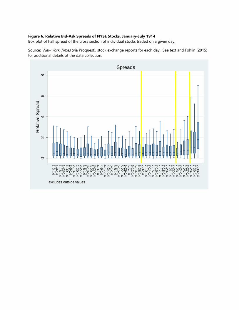
Figure 6. Relative Bid-Ask Spreads of NYSE Stocks, January-July 1914 Box plot of half spread of the cross section of individual stocks traded on a given day.

Source: New York Times (via Proquest), stock exchange reports for each day. See text and Fohlin (2015) for additional details of the data collection.

02

46

8R

elat

ive

Spre

ad

1-2-141-9-141-16-141-23-141-30-142-6-142-13-142-20-142-27-143-6-143-13-143-20-143-27-144-3-144-9-144-17-144-24-145-1-145-8-145-15-145-22-145-29-146-5-146-12-146-19-146-26-147-3-147-10-147-14-147-15-147-16-147-17-147-18-147-20-147-21-147-22-147-23-147-24-147-25-147-27-147-28-147-29-147-30-14

excludes outside values

Spreads

Figure 7. Quasi-Volatility of NYSE Stocks, January-July 1914 Box plot of quasi-volatility (high-low/last price) of the cross section of individual stocks traded on a given day.

Source: New York Times (via Proquest), stock exchange reports for each day. See text and Fohlin (2015) for additional details of the data collection.

05

1015

20qv

ol

1-2-141-9-141-16-141-23-141-30-142-6-142-13-142-20-142-27-143-6-143-13-143-20-143-27-144-3-144-9-144-17-144-24-145-1-145-8-145-15-145-22-145-29-146-5-146-12-146-19-146-26-147-3-147-10-147-14-147-15-147-16-147-17-147-18-147-20-147-21-147-22-147-23-147-24-147-25-147-27-147-28-147-29-147-30-14

excludes outside values

Volatility

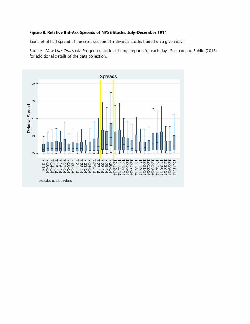
Figure 8. Relative Bid-Ask Spreads of NYSE Stocks, July-December 1914

Box plot of half spread of the cross section of individual stocks traded on a given day.

Source: New York Times (via Proquest), stock exchange reports for each day. See text and Fohlin (2015) for additional details of the data collection.

02

46

8R

elat

ive

Spre

ad

7-3-147-10-147-14-147-15-147-16-147-17-147-18-147-20-147-21-147-22-147-23-147-24-147-25-147-27-147-28-147-29-147-30-1412-12-1412-14-1412-15-1412-16-1412-17-1412-18-1412-19-1412-21-1412-22-1412-23-1412-24-1412-26-1412-28-1412-29-1412-31-14

excludes outside values

Spreads

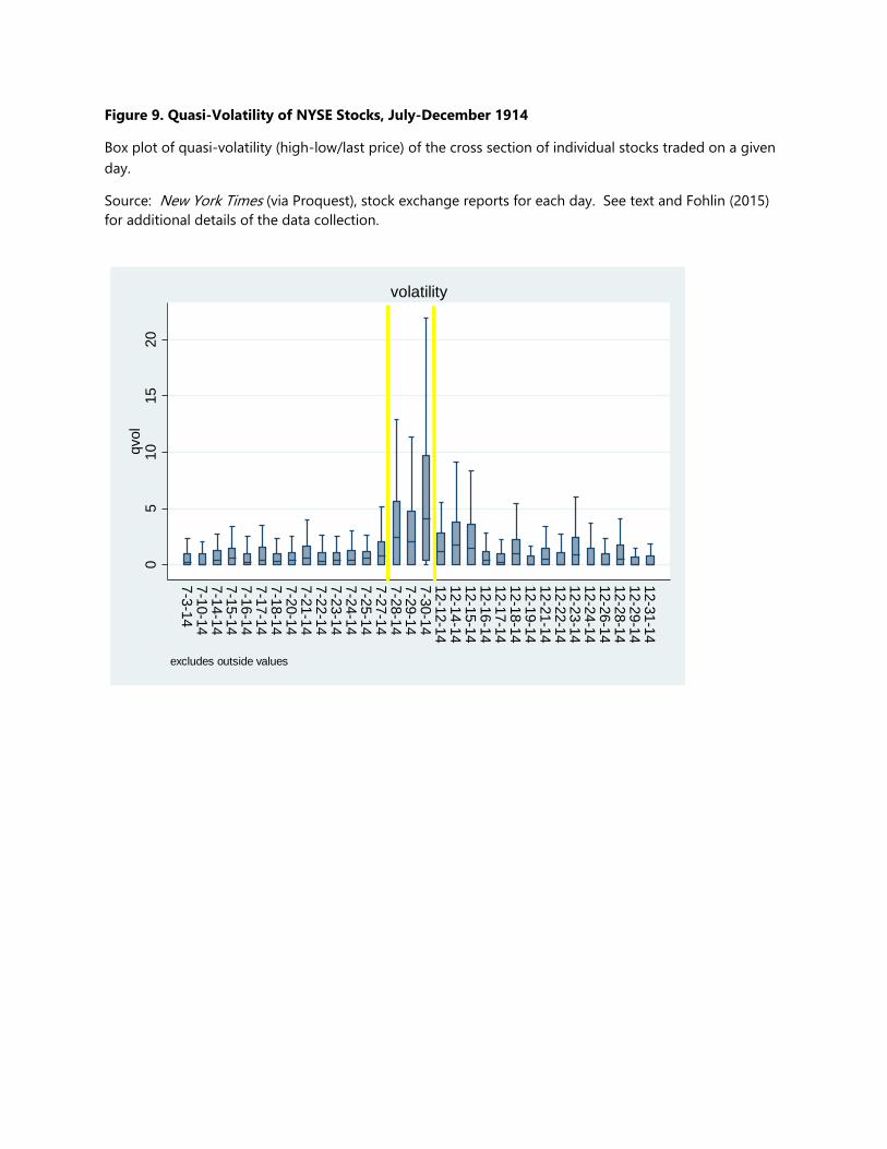
Figure 9. Quasi-Volatility of NYSE Stocks, July-December 1914

Box plot of quasi-volatility (high-low/last price) of the cross section of individual stocks traded on a given day.

Source: New York Times (via Proquest), stock exchange reports for each day. See text and Fohlin (2015) for additional details of the data collection.

05

1015

20qv

ol

7-3-147-10-147-14-147-15-147-16-147-17-147-18-147-20-147-21-147-22-147-23-147-24-147-25-147-27-147-28-147-29-147-30-1412-12-1412-14-1412-15-1412-16-1412-17-1412-18-1412-19-1412-21-1412-22-1412-23-1412-24-1412-26-1412-28-1412-29-1412-31-14

excludes outside values

volatility

Table I. Event Timeline and Time Period Comparisons

Event Event Period Control Period

Austrian Ultimatum 7/23/1914 to 7/27/1914 7/01/1914-7/22/1914

Austrian Invasion and Foreign Market Closures

7/28/1914 to 7/30/1914 7/01/1914-7/22/1914

NYSE Reopening vs. Directly Before Closure

12/15/1914 to 12/19/1914 7/28/1914 to 7/30/1914

NYSE Reopening vs. Early 1914

12/15/1914 to 12/29/1914 1/1/1914 to 6/27/1914

Table II. Summary Statistics

Statistics summarized over 17,945 stock-day observations, from January 1914-December 1915. Sales is the number of shares traded for a given day. Dollar volume is number of shares sold (“sales”) times the day’s last transaction price for a given stock (“last”). Relative half spread is ½(ask-bid)/last in percentage terms. Quasi-volatility is (high-low)/last. Market capitalization is number of shares outstanding times “last” for each day.

Source: Calculations based on data from Fohlin (2015) and New York Times (via Proquest historical collection).

Variable p25 Mean p50 p75 sd

Sales (num.) 130 3,061 500 1,900 10,695

Total sales 248,546 502,306.7 444,027 703,898 322,327

Dollar volume 8,700 230,402.2 25,000 110,250 922,749

Total dollar volume

1.86E+07 3.67E+07 3.37E+07 5.28E+07 2.36E+07

Last price 30 70.13 62.75 102 50.18

Relative half spread

0.248 1.326 0.529 1.25 2.84

Quasi-volatility

0 1.702 0.735 2.105 3.15

Market Capitalization

6,075,000 5.36E+07 1.62E+07 4.90E+07 9.28E+07

Table III. Baseline Model: Quoted Bid-Ask Spreads, Weekly (Fridays), 1914-15

Sales is the number of shares traded. Quasi-volatility is (high-low)/last (in percent). Market capitalization is number of shares outstanding*last. Regression coefficients marked with an asterisk are statistically significant (p < .05) and parentheses represent standard errors. Estimates result from a quantile (median) regression model implemented in Stata.

Source: Authors’ calculations. Data from Fohlin (2015) and New York Times (via Proquest historical collection).

Independent Variables Outcome Variables

Quantile regression Relative Spread

Ln(closing price) -0.310*** -0.314***

(0.06) (0.06)

Ln(sales) -0.161*** -0.164***

(0.0195) (0.017)

Quasi-volatility 0.0309*** 0.0305***

(0.01) (0.005)

Ln(market cap) -0.089*** -0.085***

(0.02) (0.02)

Trend 0.001**

# of week 1-104 (0.000)

Intercept 4.453*** 4.362***

(0.363) (0.359)

Observations 17,760 17,760

Adjusted R-Squared 0.209 0.209

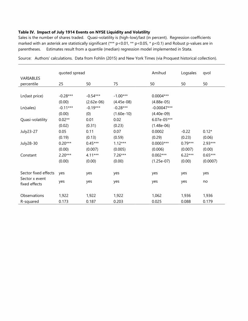
Table IV. Impact of July 1914 Events on NYSE Liquidity and Volatility Sales is the number of shares traded. Quasi-volatility is (high-low)/last (in percent). Regression coefficients marked with an asterisk are statistically significant (*** p<0.01, ** p<0.05, * p<0.1) and Robust p-values are in parentheses. Estimates result from a quantile (median) regression model implemented in Stata.

Source: Authors’ calculations. Data from Fohlin (2015) and New York Times (via Proquest historical collection).

VARIABLES

quoted spread Amihud Logsales qvol

percentile 25 50 75 50 50 50

Ln(last price) -0.28*** -0.54*** -1.00*** 0.0004*** (0.00) (2.62e-06) (4.45e-08) (4.88e-05)

Ln(sales) -0.11*** -0.19*** -0.28*** -0.00047*** (0.00) (0) (1.60e-10) (4.40e-09)

Quasi-volatility 0.02** 0.01 0.02 6.07e-05*** (0.02) (0.31) (0.23) (1.48e-06)

July23-27 0.05 0.11 0.07 0.0002 -0.22 0.12* (0.19) (0.13) (0.59) (0.29) (0.23) (0.06) July28-30 0.20*** 0.45*** 1.12*** 0.0003*** 0.79*** 2.93*** (0.00) (0.007) (0.005) (0.006) (0.007) (0.00) Constant 2.20*** 4.11*** 7.26*** 0.002*** 6.22*** 0.65*** (0.00) (0.00) (0.00) (1.25e-07) (0.00) (0.0007)

Sector fixed effects yes yes yes yes yes yes Sector x event fixed effects

yes yes yes yes yes no

Observations 1,922 1,922 1,922 1,062 1,936 1,936 R-squared 0.173 0.187 0.203 0.025 0.088 0.179

Table V. NYSE Liquidity and Volatility after NYSE Reopening, Compared to Late July Crisis Period Sales is the number of shares traded. Quasi-volatility is (high-low)/last (in percent). Regression coefficients marked with asterisks are statistically significant as follows: *** p<0.01, ** p<0.05, * p<0.1. Robust p-values are in parentheses. Estimates result from a quantile (median) regression model implemented in Stata. All models include sector fixed effects and (sector x event) fixed effects.

Source: Authors’ calculations. Data from Fohlin (2015) and New York Times (via Proquest historical collection).

VARIABLES Relative spread Amihud Logsales qvol 25 50 75 50 50 50 Ln(last price) -0.41*** -0.72*** -1.34***

0.0006***

(0.00) (0.00) (0.00)

(0.00)

Ln(sales) -0.20*** -0.33*** -0.43***

-0.001***

(0.00) (0.00) (0.00)

(0.00)

Quasi-volatility 0.03*** (0.00)

0.03 (0.24)

0.03 (0.12)

0.0001*** (0.00)

Dec. 15-19 v. Jul 28-30

-0.18** (0.02)

-0.53*** (0.00)

-1.47*** (0.00)

-0.001*** (0.00)

-1.01*** (0.002)

-2.29*** (0.00)

Constant 3.65*** 6.48*** 11.26*** 0.004*** 7.00*** 2.94*** (0.00) (0.00) (0.00) (0.00) (0.00) (0.00) Observations 909 909 909 734 937 937 R-squared 0.22 0.24 0.24 0.02 0.13 0.13

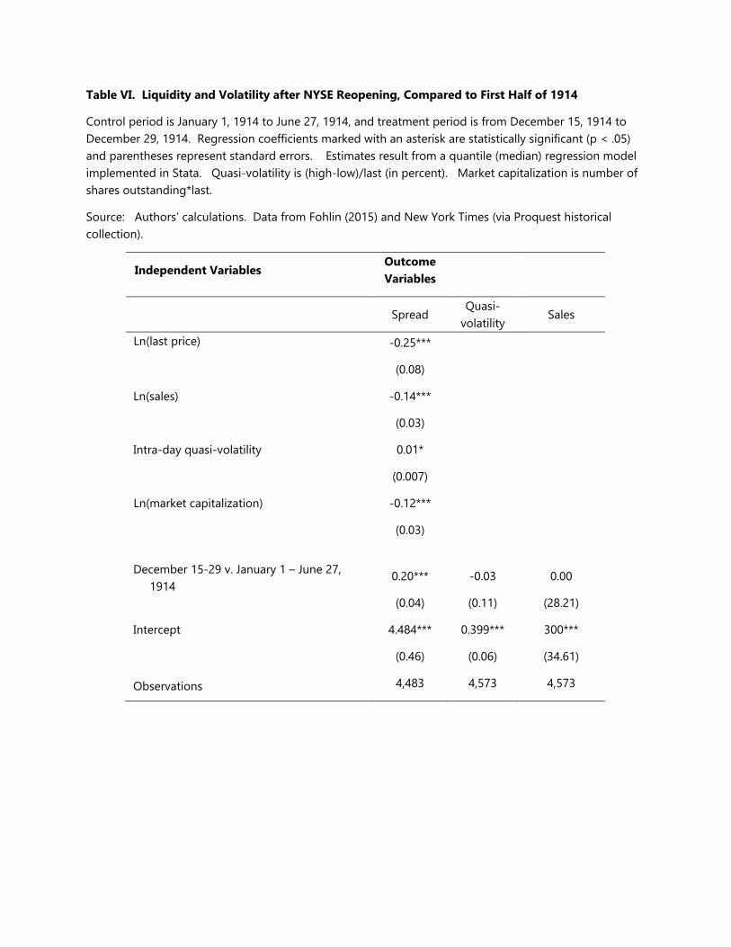
Table VI. Liquidity and Volatility after NYSE Reopening, Compared to First Half of 1914

Control period is January 1, 1914 to June 27, 1914, and treatment period is from December 15, 1914 to December 29, 1914. Regression coefficients marked with an asterisk are statistically significant (p < .05) and parentheses represent standard errors. Estimates result from a quantile (median) regression model implemented in Stata. Quasi-volatility is (high-low)/last (in percent). Market capitalization is number of shares outstanding*last.

Source: Authors’ calculations. Data from Fohlin (2015) and New York Times (via Proquest historical collection).

Independent Variables Outcome Variables

Spread Quasi-

volatility Sales

Ln(last price)

-0.25***

(0.08)

Ln(sales)

-0.14***

(0.03)

Intra-day quasi-volatility

0.01*

(0.007)

Ln(market capitalization)

-0.12***

(0.03)

December 15-29 v. January 1 – June 27, 1914

0.20***

(0.04)

-0.03

(0.11)

0.00

(28.21)

Intercept 4.484***

(0.46)

0.399***

(0.06)

300***

(34.61)

Observations 4,483 4,573 4,573

Table VII. “International in Character” Securities Comparative Characteristics

Regression coefficients marked with an asterisk are statistically significant (p < .05) and parentheses represent standard errors. Estimates result from a quantile (median) regression model implemented in Stata. Quasi-volatility is (high-low)/last (in percent). Market capitalization is number of shares outstanding*last. International indicates stocks denotes as “International in Character” by the NYSE.

Source: Authors’ calculations. Data from Fohlin (2015) and New York Times (via Proquest historical collection).

Independent Variables

Outcome Variables

Robust Regression Spread Market Cap (thousands)

qvol Total sales

Ln(last price)

-0.24*** (0.04)

Ln(sales)

-0.15*** (0.01)

Intra-day quasi-

volatility

0.02*** (0.004)

Ln(market

capitalization)

-0.07*** (0.02)

International 0.06 862,956 -0.67*** -434.7***

(0.04) (1.128e+06) (0.21) (88.80)

Intercept 3.80*** 1.443e+07*** 2.38*** 1,046***

(0.22) (756,938) (0.14) (59.57)

Observations 809 820 820 820

Adjusted R^2 0.391 0.001 0.013 0.028

Table VIII. “International in Character” Securities Comparative Characteristics

Quasi-volatility is (high-low)/last (in percent). Market capitalization is number of shares outstanding*last. International indicates stocks denotes as “International in Character” by the NYSE. Models include sector fixed effects. Robust p-values are in parentheses (*** p<0.01, ** p<0.05, *p<0.1).

Source: Authors’ calculations. Data from Fohlin (2015) and New York Times (via Proquest historical collection).

VARIABLES Pooled probit

Panel probit

Relative half spread 0.0229* -0.0313

(0.0747) (0.546)

Ln(last price) 0.503*** 0.372

(3.86e-05) (0.287)

Ln(sales) -0.0343 -0.112

(0.470) (0.505)

Quasi-volatility 0.0163 0.0144

(0.183) (0.711)

Market capitalization -4.51e-10 -5.67e-

10

(0.733) (0.877)

Constant -2.015*** -0.915

(7.31e-05) (0.472)

Observations 16,065 16,065

Table IX. International in Character Stocks

The first three columns test the effect of breaks at the Austrian Ultimatum (July 23-27) and Austrian invasion of Serbia and subsequent market closures in Europe (July 28-30) versus the rest of July 1914. The latter three columns test for a break at the reopening of the exchange compared to the last three days before the closure (Dec 15-19 v. July 28-30). Quasi-volatility is (high-low)/last (in percent). Market capitalization is number of shares outstanding*last. International indicates stocks denotes as “International in Character” by the NYSE.

Source: Authors’ calculations. Data from Fohlin (2015) and New York Times (via Proquest historical collection).

Austrian Ultimatum and Invasion Reopening of the NYSE (1) (2) (3) (4) (5) (6)

VARIABLES Relative spread qvol Logsales

Relative spread qvol Logsales

Ln(Last price) -0.52*** -0.71*** (1.42e-05) (0.00)

Ln(Sales) -0.19*** -0.32*** (0.00) (0.00)

Quasi-volatility 0.01 0.02*** (0.17) (0.00)

Event (1) 0.14*** 0.10 -0.00 -0.77*** -3.39*** -1.14***

(0.01) (0.28) (1.00) (0.00) (0.00) (3.66e-10)

Event (2) 0.72*** 3.42*** 0.92*** (2.96e-09) (0.00) (1.10e-08)

International 0.10 -0.25 -0.29 -0.08 -1.85** -0.22

(0.27) (0.24) (0.17) (0.54) (0.02) (0.53)

International * event -0.013 0.13 0.29 0.15 1.72** 0.16

(0.87) (0.44) (0.17) (0.29) (0.02) (0.62)

International * event 2 -0.11 -1.60*** 0.06 (0.46) (0.004) (0.84)

Constant 3.87*** 0.59*** 5.99*** 6.407*** 4.01*** 6.91***

(7.93e-11) (3.61e-09) (0.00) (0.00) (0.00) (0.00)

R-squared 0.198 0.174 0.043 0.229 0.108 0.088 Observations 1,922 1,936 1,936 909 937 937