When is a copula constant? A test for changing relationships · Kendall™s Tau will change when...
114
When is a copula constant? A test for changing relationships Fabio Busetti and Andrew Harvey Bank of Italy and University of Cambridge November 2007 Busetti and Harvey (Bank of Italy and University of Cambridge) When is a copula constant? November 2007 1 / 54
Transcript of When is a copula constant? A test for changing relationships · Kendall™s Tau will change when...

When is a copula constant? A test for changingrelationships
Fabio Busetti and Andrew Harvey
Bank of Italy and University of Cambridge
November 2007
Busetti and Harvey (Bank of Italy and University of Cambridge)When is a copula constant? November 2007 1 / 54

Introduction
Understanding and measuring the relationship between movements indi¤erent assets plays a key role in designing a portfolio. Themultivariate normal distribution is not usually suitable for this task fortwo reasons:
asset returns are not normally distributed, and,their comovements are not adequately captured by correlationcoe¢ cients.
The second of these points has led to an explosion of interest incopulas. A copula models the relationships between variablesindependently of their marginal distributions. It does so by means of ajoint distribution function with uniform marginals, obtained from thedistribution functions of the original marginals.
Busetti and Harvey (Bank of Italy and University of Cambridge)When is a copula constant? November 2007 2 / 54

The stock returns data used as illustrations are General Motors andIBM daily returns from April 7th, 1986, to April 7th, 1999.
25.0 22.5 20.0 17.5 15.0 12.5 10.0 7.5 5.0 2.5 0.0 2.5 5.0 7.5 10.0 12.5
20
15
10
5
0
5
10
GM × IBM
Busetti and Harvey (Bank of Italy and University of Cambridge)When is a copula constant? November 2007 3 / 54

Empirical copula for GM and IBM
Instead of considering the original variables, we consider the pairs ofcorresponding ranks.A plot of these ranks, re-scaled by dividing by one plus the samplesize, forms the domain of the empirical copula.
0.0 0.1 0.2 0.3 0.4 0.5 0.6 0.7 0.8 0.9 1.0
0.1
0.2
0.3
0.4
0.5
0.6
0.7
0.8
0.9
1
Ranks of GM returns
Ran
ks o
f IB
M r
etur
ns
Figure: Domain of the empirical copula for GM and IBM
Figure 1 shows the domain of the empirical copula for GM and IBM. Thecorrelation is r = 0.377, while Kendall�s tau is 0.216.
Busetti and Harvey (Bank of Italy and University of Cambridge)When is a copula constant? November 2007 4 / 54

The strength of the relationship between two variables can bemeasured by Kendall�s-Tau. Kendall�s-Tau is computed from ranksand is more appropriate as a measure of concordance than acorrelation coe¢ cient. The dependence parameter for some simplecopulas can be shown to be a function of Kendall�s-Tau.
If the relationship between two variables changes over time thenKendall�s Tau will change when computed from di¤erent subsamples.
Evidence that this might happen is provided by Van Der Goorbergha,Genest and Werker (2005) and Patton (2006). Cherubini et al(p.179) report time-varying correlation in a Gaussian copula.
Busetti and Harvey (Bank of Italy and University of Cambridge)When is a copula constant? November 2007 5 / 54

To get an idea of possible changes in the relationship we divided the�rst 3000 observations up into 6 group of 500, that is 1 to 500, 501to 1000, and so on. This leaves the �nal group from 3001 to 3392.
The correlation coe¢ cients and Kendall�s tau are given in the tablebelow. It is interesting that the correlations are higher at thebeginning than at the end. There certainly appears to be aconsiderable degree of movement, but we need to know if it isstatistically signi�cant.
1 2 3 4 5 6 7r .74 .51 .42 .16 .18 .10 .36Tau .37 .34 .26 .10 .15 .08 .22
Busetti and Harvey (Bank of Italy and University of Cambridge)When is a copula constant? November 2007 6 / 54

0.0 0.2 0.4 0.6 0.8 1.0
0.5
1.0 Obs: 1500; τ = 0.37; ρ = 0.74
0.0 0.2 0.4 0.6 0.8 1.0
0.5
1.0 Obs: 5011000; τ = 0.34; ρ = 0.51
0.0 0.2 0.4 0.6 0.8 1.0
0.5
1.0 Obs: 10011500; τ = 0.26; ρ = 0.42
0.0 0.2 0.4 0.6 0.8 1.0
0.5
1.0 Obs: 15012000; τ = 0.10; ρ = 0.16
0.0 0.2 0.4 0.6 0.8 1.0
0.5
1.0 Obs: 20012500; τ = 0.15; ρ = 0.18
0.0 0.2 0.4 0.6 0.8 1.0
0.5
1.0 Obs: 25013000; τ = 0.08; ρ = 0.10
0.0 0.2 0.4 0.6 0.8 1.0
0.5
1.0 Obs: 30013392; τ = 0.22; ρ = 0.36
Figure: Empirical copulas for GM and IBM
Busetti and Harvey (Bank of Italy and University of Cambridge)When is a copula constant? November 2007 7 / 54

The aim is to develop a suite of tests for changes in di¤erent parts of thecopula, as well as an overall test for changing dependence.
These tests do not require a model for the copula
They can be regarded as an extension of the stationarity tests fortime-varying quantiles proposed in Busetti and Harvey (2007).
The time-varying quantile test are constructed from time series ofindicator variables.
Busetti and Harvey (Bank of Italy and University of Cambridge)When is a copula constant? November 2007 8 / 54

Consider the proportion of cases in which the observations lie below aparticular quantile in both series. The question is whether thisproportion is constant over time.
Looking at di¤erent quantiles allows us to focus on di¤erent aspectsof the relationship.
Changing dependence may be of particular importance in the lowertails, because of its relevance for the value at risk (VaR) of a portfolio.We might also consider the question of whether a single test, based onthe quadrants formed from the two medians, is useful as an overall testof changing concordance.
Busetti and Harvey (Bank of Italy and University of Cambridge)When is a copula constant? November 2007 9 / 54

Consider the proportion of cases in which the observations lie below aparticular quantile in both series. The question is whether thisproportion is constant over time.
Looking at di¤erent quantiles allows us to focus on di¤erent aspectsof the relationship.
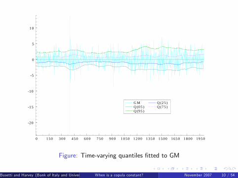
Changing dependence may be of particular importance in the lowertails, because of its relevance for the value at risk (VaR) of a portfolio.
We might also consider the question of whether a single test, based onthe quadrants formed from the two medians, is useful as an overall testof changing concordance.
Busetti and Harvey (Bank of Italy and University of Cambridge)When is a copula constant? November 2007 9 / 54

Consider the proportion of cases in which the observations lie below aparticular quantile in both series. The question is whether thisproportion is constant over time.
Looking at di¤erent quantiles allows us to focus on di¤erent aspectsof the relationship.
Changing dependence may be of particular importance in the lowertails, because of its relevance for the value at risk (VaR) of a portfolio.We might also consider the question of whether a single test, based onthe quadrants formed from the two medians, is useful as an overall testof changing concordance.
Busetti and Harvey (Bank of Italy and University of Cambridge)When is a copula constant? November 2007 9 / 54
0 1 5 0 3 0 0 4 5 0 6 0 0 7 5 0 9 0 0 1 0 5 0 1 2 0 0 1 3 5 0 1 5 0 0 1 6 5 0 1 8 0 0 1 9 5 0
2 0
1 5
1 0
5
0
5
1 0
G MQ (0 5 )Q (9 5 )
Q (2 5 )Q (7 5 )
Figure: Time-varying quantiles �tted to GM
Busetti and Harvey (Bank of Italy and University of Cambridge)When is a copula constant? November 2007 10 / 54

Quantiles and Quantics
Let ξ(τ) denote the τ � th quantile. The probability that anobservation is less than ξ(τ) is τ, where 0 < τ < 1. Given a set of Tobservations, yt , t = 1, ..,T , the sample quantile, eξ(τ), can beobtained by sorting the observations in ascending order.
The residuals associated with a quantile may be coded as indicators.The τ�quantile indicator is
IQ(yt � ξ(τ)) =
�τ � 1, if yt < ξ(τ)
τ, if yt > ξ(τ), t = 1, ...,T (1)
Note that IQ(0) is not determined but we will constrain it to lie in therange [τ � 1, τ].
If ξ(τ) is the unique population τ�quantile and y has a continuouspositive density in the neighbourhood of ξ(τ), then IQ(yt � ξ(τ))has a mean of zero and a variance of τ(1� τ).The sample τ�quantile indicator, or τ�quantic, at time t is
IQ(yt � eξ(τ)), t = 1, ...,T .The quantics sum to zero.
Busetti and Harvey (Bank of Italy and University of Cambridge)When is a copula constant? November 2007 11 / 54

Quantiles and Quantics
Let ξ(τ) denote the τ � th quantile. The probability that anobservation is less than ξ(τ) is τ, where 0 < τ < 1. Given a set of Tobservations, yt , t = 1, ..,T , the sample quantile, eξ(τ), can beobtained by sorting the observations in ascending order.The residuals associated with a quantile may be coded as indicators.The τ�quantile indicator is
IQ(yt � ξ(τ)) =
�τ � 1, if yt < ξ(τ)
τ, if yt > ξ(τ), t = 1, ...,T (1)
Note that IQ(0) is not determined but we will constrain it to lie in therange [τ � 1, τ].
If ξ(τ) is the unique population τ�quantile and y has a continuouspositive density in the neighbourhood of ξ(τ), then IQ(yt � ξ(τ))has a mean of zero and a variance of τ(1� τ).
The sample τ�quantile indicator, or τ�quantic, at time t isIQ(yt � eξ(τ)), t = 1, ...,T .
The quantics sum to zero.
Busetti and Harvey (Bank of Italy and University of Cambridge)When is a copula constant? November 2007 11 / 54

Quantiles and Quantics
Let ξ(τ) denote the τ � th quantile. The probability that anobservation is less than ξ(τ) is τ, where 0 < τ < 1. Given a set of Tobservations, yt , t = 1, ..,T , the sample quantile, eξ(τ), can beobtained by sorting the observations in ascending order.The residuals associated with a quantile may be coded as indicators.The τ�quantile indicator is
IQ(yt � ξ(τ)) =
�τ � 1, if yt < ξ(τ)
τ, if yt > ξ(τ), t = 1, ...,T (1)
Note that IQ(0) is not determined but we will constrain it to lie in therange [τ � 1, τ].
If ξ(τ) is the unique population τ�quantile and y has a continuouspositive density in the neighbourhood of ξ(τ), then IQ(yt � ξ(τ))has a mean of zero and a variance of τ(1� τ).The sample τ�quantile indicator, or τ�quantic, at time t is
IQ(yt � eξ(τ)), t = 1, ...,T .The quantics sum to zero.Busetti and Harvey (Bank of Italy and University of Cambridge)When is a copula constant? November 2007 11 / 54

Tests based on quantics
A test of the null hypothesis that the τ�quantile is constant may bebased on the quantics.
If the alternative hypothesis is that the τ�quantile follows a randomwalk, a modi�ed version of the stationarity test of Nyblom andMäkeläinen (1983) is appropriate.
ητ(Q) =1
T 2τ(1� τ)
T
∑t=1
t
∑i=1IQ(yt � eξ(τ))!2
Asymptotic distribution is Cramér-von Mises (CvM); the 5% critical valueis 0.461.
Busetti and Harvey (Bank of Italy and University of Cambridge)When is a copula constant? November 2007 12 / 54

Nyblom and Harvey (2001) show that the test has high power againstan integrated random walk, which when �tted yields a curve close toa cubic spline.
Harvey and Streibel (1998) show that it has an LBI interpretationagainst a highly persistent stationary �rst-order autoregression
Nyblom (1989) shows test has power against a break, or breaks, in anotherwise stationary time series.
Long-run variance corrects size when quantile is stationary.
Busetti and Harvey (Bank of Italy and University of Cambridge)When is a copula constant? November 2007 13 / 54

Joint test for the time invariance of a distribution
A joint test to see if a group of N quantiles show evidence ofchanging over time can be based on a generalisation of (2), namely
ητ(Q;N) = T�2
T
∑t=1
"t
∑i=1IQi
#0S�1
"t
∑i=1IQi
#, (2)
where the j � th element of the N � 1 vector IQi isIQ(yi � eξ(τj )) and the jk � th element of the N �N covariancematrix S is τj (1� τk ) for τk > τj .
Under the null hypothesis of IID observations, the limiting distribution ofητ(Q;N) is Cramér-von Mises with N degrees of freedom, denotedCvM(N).
Busetti and Harvey (Bank of Italy and University of Cambridge)When is a copula constant? November 2007 14 / 54

Bivariate series
Consider a bivariate series, y1t and y2t , t = 1, ...,T . By convertingto ranks we can obtain the sample quantiles and the empirical copula.The empirical copula yields the proportion of cases in which bothobservations in a pair are less than, or equal to, particular quantiles,eξ(τ1) and eξ(τ2). This proportion will be denoted as CT (τ1, τ2).The tests in Busetti and Harvey (2007) were designed to detectmovements in the quantiles of the distributions of univariate series. Ifthere are two series and their marginal distributions are constant, wecan move on to address the question of whether their copula ischanging over time.
As with univariate series, the tests are based on indicators, but wenow have to consider combinations of quantiles from the two series.
Busetti and Harvey (Bank of Italy and University of Cambridge)When is a copula constant? November 2007 15 / 54
Bivariate series
To simplify matters, we will set τ1 = τ2 = τ, 0 < τ < 1, and explorethe possibility of movements C (τ, τ), the probability that bothobservations lie below their respective τ�quantiles.
Since there are four quadrants associated with a given τ, someattention needs to be paid to the other three. The probability thatboth observations lie above their respective τ�quantiles is known asthe survival function, and denoted C (τ, τ). It is equal to1� 2τ + C (τ, τ). The probabilities of being in the other twoquadrants are the same, namely τ � C (τ, τ).
Busetti and Harvey (Bank of Italy and University of Cambridge)When is a copula constant? November 2007 16 / 54

Bivariate series
To simplify matters, we will set τ1 = τ2 = τ, 0 < τ < 1, and explorethe possibility of movements C (τ, τ), the probability that bothobservations lie below their respective τ�quantiles.Since there are four quadrants associated with a given τ, someattention needs to be paid to the other three. The probability thatboth observations lie above their respective τ�quantiles is known asthe survival function, and denoted C (τ, τ). It is equal to1� 2τ + C (τ, τ). The probabilities of being in the other twoquadrants are the same, namely τ � C (τ, τ).
Busetti and Harvey (Bank of Italy and University of Cambridge)When is a copula constant? November 2007 16 / 54

Copulas and concordance
The value of C (τ, τ) indicates the strength of dependence at τ. Withperfect concordance, C (τ, τ) = τ and C (τ, τ) = 1� τ, while withperfect discordance both these probabilities are zero. For independentseries, C (τ, τ) = τ2, while C (τ, τ) = (1� τ)2, and the probabilitiesof being in one of the other quadrants are both τ(1� τ).
Summing C (τ, τ) and C (τ, τ) gives a simple measure of whatKruskal (1958, p 818) calls quadrant association.
Busetti and Harvey (Bank of Italy and University of Cambridge)When is a copula constant? November 2007 17 / 54

As an illustration, the Clayton copula is de�ned in terms of uniformvariates, u1 and u2, as
C (u1, u2) = (u�θ1 + u�θ
2 � 1)�1/θ, θ 2 [�1,∞)
and for a given τ, C (τ, τ)/τ =�2� τθ
��1/θ. For θ = 1 and a small
τ, C (τ, τ) ' τ/2.
The Clayton copula is asymmetric in that the upper tail probabilityfor 1� τ, that is the survival copula, C (1� τ, 1� τ), is not the sameas C (τ, τ). The relationship is
C (1� τ, 1� τ) = 1� 2(1� τ) + C (1� τ, 1� τ)
= 2τ � 1+ (1� τ)(2� (1� τ)θ)�1/θ
For θ = 1, we get 2τ� 1+ (1� τ)(1+ τ)�1. This is .018 for τ = .1,while for τ = .05, it is .0048. These probabilities are much smallerthan those for the lower tail.
Busetti and Harvey (Bank of Italy and University of Cambridge)When is a copula constant? November 2007 18 / 54

As an illustration, the Clayton copula is de�ned in terms of uniformvariates, u1 and u2, as
C (u1, u2) = (u�θ1 + u�θ
2 � 1)�1/θ, θ 2 [�1,∞)
and for a given τ, C (τ, τ)/τ =�2� τθ
��1/θ. For θ = 1 and a small
τ, C (τ, τ) ' τ/2.The Clayton copula is asymmetric in that the upper tail probabilityfor 1� τ, that is the survival copula, C (1� τ, 1� τ), is not the sameas C (τ, τ). The relationship is
C (1� τ, 1� τ) = 1� 2(1� τ) + C (1� τ, 1� τ)
= 2τ � 1+ (1� τ)(2� (1� τ)θ)�1/θ
For θ = 1, we get 2τ� 1+ (1� τ)(1+ τ)�1. This is .018 for τ = .1,while for τ = .05, it is .0048. These probabilities are much smallerthan those for the lower tail.
Busetti and Harvey (Bank of Italy and University of Cambridge)When is a copula constant? November 2007 18 / 54

Clayton Copula
Figure: CDF of the Claytoncopula
Figure: PDF of the Claytoncopula
Busetti and Harvey (Bank of Italy and University of Cambridge)When is a copula constant? November 2007 19 / 54

Bivariate series
The coe¢ cients of tail dependence are measures of pairwisedependence that depend on the copula. The coe¢ cient of lower taildependence is limτ!0 C (τ, τ)/τ, while the coe¢ cient of upper taildependence is limτ!1 C (τ, τ)/(1� τ).
If two variables have a bivariate normal distribution, they areasymptotically independent in the tails as the coe¢ cients of taildependence are both zero. On the other hand, a t-copula does exhibittail dependence. For θ > 0, the Clayton copula exhibits lower taildependence, that is limτ!0 C (τ, τ)/τ = 2�1/θ, and as θ ! ∞, thiscoe¢ cient tends to one.
Busetti and Harvey (Bank of Italy and University of Cambridge)When is a copula constant? November 2007 20 / 54

Bivariate quantics
We will de�ne the bivariate τ�quantic - or τ�bi-quantic - as
BIQ(y1t � eξ1(τ), y2t � eξ2(τ)) (3)
= CT (τ, τ)� I (y1t � eξ1(τ), y2t � eξ2(τ)), t = 1, ...,T
where I (.) is the indicator function.
By construction this has a mean of zero and a variance ofCT (τ, τ)(1� CT (τ, τ)). When there is no ambiguity we willabbreviate BIQ(y1t � eξ1(τ), y2t � eξ2(τ) to BIQ(τ).
Associated with BIQ(τ) are three complementary bivariateτ�quantics. The �rst is
BIQ(y1t > eξ1(τ), y2t > eξ2(τ)) (4)
= CT (τ, τ)� I (y1t > eξ1(τ), y2t > eξ2(τ)) (5)
Busetti and Harvey (Bank of Italy and University of Cambridge)When is a copula constant? November 2007 21 / 54

We call this the survival τ�quantic and use the shorthand notationBIQ(τ).
Remember that CT (τ, τ) = 1� 2τ + CT (τ, τ). The variance ofBIQ(τ) is CT (τ, τ)(1� CT (τ, τ)).
The other two complementary τ�bi-quantics are
BIQ(y1t � eξ1(τ), y2t > eξ2(τ)) (6)
= C�T (τ, τ)� I (y1t � eξ1(τ), y2t > eξ2(τ)) (7)
and
BIQ(y1t > eξ1(τ), y2t � eξ2(τ)) (8)
= C�T (τ, τ)� I (y1t > eξ1(τ), y2t � eξ2(τ)) (9)
where C�T (τ, τ) = τ � CT (τ, τ).
Busetti and Harvey (Bank of Italy and University of Cambridge)When is a copula constant? November 2007 22 / 54

Tests
We now consider tests of the null hypothesis that C (τ, τ) is constant.Test statistics can be formed from the bi-quantics in the same way as forthe quantics.
Thus, for a given τ,
ητ(BQ;BB) =1
T 2CT (τ, τ)(1� CT (τ, τ))T
∑t=1
t
∑i=1BIQ(τ)
!2(10)
The asymptotic distribution of this stationarity test statistic when theseries are jointly stationary is Cramér von Mises. Since there are limitson the range of C (τ, τ) the alternative the alternative hypothesis isbest thought of as one in which C (τ, τ) is slowly changing, or subjectto breaks, rather than being a random walk.
In the Monte Carlo experiments, the test based on (10) is denotedBB to signify that the indicator is unity when both observations arebelow their respective quantiles. The test constructed using thesurvival bi-quantics is denoted AA.
Busetti and Harvey (Bank of Italy and University of Cambridge)When is a copula constant? November 2007 23 / 54

A combined test can be constructed from any three bi-quantics,provided that CT (τ, τ) < τ. The statistic is
ητ(BQ; 3) = T�2
T
∑t=1
"t
∑i=1BIQi
#0S�1
"t
∑i=1BIQi
#, (11)
where the elements of the 3� 1 vector BIQi are chosen from (3),(4), (6) and (8), and S is their sample covariance matrix. Under thenull hypothesis of serially independent observations with a constantcopula, the limiting distribution of ητ(BQ; 3) is Cramér-von Miseswith 3 degrees of freedom.
We can add BIQ(τ)and BIQ(τ) to give
BIQ(τ) + BIQ(τ)
= 1� 2τ + 2CT (τ, τ)� I (y1t � eξ1(τ), y2t � eξ2(τ) or y1t > eξ1(τ), y2t > eξ2(τ)).A test statistic formed from this series will be denoted ητ(BQ + BQ).Since it is based on the sum of CT (τ, τ) and CT (τ, τ), we will call it thequadrant association test. Its limiting distribution under the nullhypothesis is Cramér-von Mises with one degree of freedom.
Busetti and Harvey (Bank of Italy and University of Cambridge)When is a copula constant? November 2007 24 / 54

Single comprehensive tests of changing dependence
If a single overall test is required, it may be based on the combined orquadrant association tests for τ = 0.5.
We might compare the power of these tests with a stationarity basedon the series
(y1t � y1)(y2t � y2), t = 1, ...,T
We call this the changing correlation test. Its performance willdepend on the whole joint distribution, not just the copula.
The tests based on τ = 0.5 could be extended to joint tests based ona range of τ0s.
Busetti and Harvey (Bank of Italy and University of Cambridge)When is a copula constant? November 2007 25 / 54

Bi-quantilogram
The pattern of serial correlation can be captured by computing thecorrelograms of the bivariate τ�quantics. These might be calledbi-quantilograms.
They are not the same as the cross-quantilograms of Linton andWhang (2007), though these may also be useful.
Box-Ljung Q-statistics may be formed from the bi-quantilograms andused as an alternative to stationarity tests for assessing change in thecopula.
Busetti and Harvey (Bank of Italy and University of Cambridge)When is a copula constant? November 2007 26 / 54

Monte Carlo
We consider three cases of data generating processes, denoted byA,B,C; the �rst two are based on a time-varying Gaussian copulawhile the third is characterized by a Clayton copula, with lower taildependence. In general the two degree of freedom test was dominatedby the others and so we do not report the results for it.
The speed of convergence to the asymptotic distribution may be slowwhen τ is close to zero or one. The simulation experiments thereforedo not include τ = 0.10 or 0.05. For larger sample sizes the relativeperformances of the tests should be similar to what we report here forfor τ = .25, 0.5 and 0.75.
All tests are at the 5% signi�cance level.
Busetti and Harvey (Bank of Italy and University of Cambridge)When is a copula constant? November 2007 27 / 54

Monte Carlo A
The observations are generated from a bivariate Gaussian distributionwith time varying correlation
ρt =1� eµt
1+ eµt,
where µt is a random walk process obtained from Gaussianinnovations with mean zero and variance equal to q2. Logistic - soρt 2 (�1, 1).
Table (1) - Power is a maximum at τ = .5. The lower quadrant test,BB, is more powerful for τ < 0.5, while the upper quadrant test, AA,is more powerful for τ > 0.5. Furthermore the power for BB at τ isthe same as the power for AA at 1� τ; this is a re�ection of thesymmetry properties of the Gaussian distribution.
The table shows that the bi-quantic tests are signi�cantly morepowerful than the Box-Ljung bi-quantilogram Q(m)-tests.
Busetti and Harvey (Bank of Italy and University of Cambridge)When is a copula constant? November 2007 28 / 54

Monte Carlo A
The observations are generated from a bivariate Gaussian distributionwith time varying correlation
ρt =1� eµt
1+ eµt,
where µt is a random walk process obtained from Gaussianinnovations with mean zero and variance equal to q2. Logistic - soρt 2 (�1, 1).Table (1) - Power is a maximum at τ = .5. The lower quadrant test,BB, is more powerful for τ < 0.5, while the upper quadrant test, AA,is more powerful for τ > 0.5. Furthermore the power for BB at τ isthe same as the power for AA at 1� τ; this is a re�ection of thesymmetry properties of the Gaussian distribution.
The table shows that the bi-quantic tests are signi�cantly morepowerful than the Box-Ljung bi-quantilogram Q(m)-tests.
Busetti and Harvey (Bank of Italy and University of Cambridge)When is a copula constant? November 2007 28 / 54

The lower part of the table contains the results for the combined test,ητ(BQ; 3), the quadrant association test, ητ(BQ + BQ), and thetest of changing correlation. All of them appear to be more powerfulthan the single quadrant bi-quantic tests.
The quadrant association test appears to be more powerful than thecombined test for τ = 0.50. For small values of q the maximumpower is attained by the test of changing correlation, but thequadrant association test is better for q = 0.25 and above.
Busetti and Harvey (Bank of Italy and University of Cambridge)When is a copula constant? November 2007 29 / 54

Figure: Table 1
Busetti and Harvey (Bank of Italy and University of Cambridge)When is a copula constant? November 2007 30 / 54

Monte Carlo B
The observations are generated from a bivariate Gaussian distributionwith a structural break in the correlation coe¢ cient. We set ρt = .75in the �rst half of the sample and ρt = .75, .50, .25, 0 in the secondhalf. T = 200.
Table 2 - Again the copula bi-quantic tests are signi�cantly morepowerful than those based on the bi-quantilogram, but the di¤erencesappear to be even greater.
Broadly speaking, these results are qualitatively the same as thoseobtained (A).
Busetti and Harvey (Bank of Italy and University of Cambridge)When is a copula constant? November 2007 31 / 54

Figure: Table 2
Busetti and Harvey (Bank of Italy and University of Cambridge)When is a copula constant? November 2007 32 / 54

Monte Carlo C
Table (3) - Clayton copula with structural break in the dependenceparameter.
No longer symmetry in the BB and AA tests, though the BA and ABtests do, as before, have similar power. In fact these tests are nowmore powerful than the the BB and AA tests.
As before the bi-quantilogram tests are signi�cantly less powerful.
The quadrant association test is the most powerful test overall -better than the combined bi-quantic tests.
The test of changing correlation has very low power.
Busetti and Harvey (Bank of Italy and University of Cambridge)When is a copula constant? November 2007 33 / 54

Di¤erent marginals would give di¤erent results for the changingcorrelation test, but unless the joint distribution is bivariate normal, itseems that a good performance cannot be guaranteed.
Taking all three sets of results together, the quadrant association testwith τ = 0.5 is clearly the one to be recommended for detectingoverall changes in dependence. It also seems to be the preferred testfor other values of τ.
Busetti and Harvey (Bank of Italy and University of Cambridge)When is a copula constant? November 2007 34 / 54

Figure: Table 3
Busetti and Harvey (Bank of Italy and University of Cambridge)When is a copula constant? November 2007 35 / 54

Correcting for time variation in the individual series
The bi-quantic tests will tend to reject if the individual quantiles aretime-varying. Even if stationary will still reject with non-parametriccorrection if persistent.
If the movements in quantiles are due solely to changes in volatility,the series may be adjusted by dividing by a measure of dispersion.A stochastic volatility (SV) model can be �tted to each of the seriesand the resulting (two sided) smoothed estimates of the standarddeviations used to rescale the observations.Alternatively could rescale the observations by a time-varyingestimate of the interquartile range, using the approach of De Rossiand Harvey (2006).More generally time-varying τ�quantiles could be �tted, as in DeRossi and Harvey (2006), and the bi-quantics formed from them.For an overall quadrant association test based on τ = 0.5, there is noneed to make any adjustments if the medians can be assumedconstant.
Busetti and Harvey (Bank of Italy and University of Cambridge)When is a copula constant? November 2007 36 / 54

Correcting for time variation in the individual series
The bi-quantic tests will tend to reject if the individual quantiles aretime-varying. Even if stationary will still reject with non-parametriccorrection if persistent.If the movements in quantiles are due solely to changes in volatility,the series may be adjusted by dividing by a measure of dispersion.
A stochastic volatility (SV) model can be �tted to each of the seriesand the resulting (two sided) smoothed estimates of the standarddeviations used to rescale the observations.Alternatively could rescale the observations by a time-varyingestimate of the interquartile range, using the approach of De Rossiand Harvey (2006).More generally time-varying τ�quantiles could be �tted, as in DeRossi and Harvey (2006), and the bi-quantics formed from them.For an overall quadrant association test based on τ = 0.5, there is noneed to make any adjustments if the medians can be assumedconstant.
Busetti and Harvey (Bank of Italy and University of Cambridge)When is a copula constant? November 2007 36 / 54

Correcting for time variation in the individual series
The bi-quantic tests will tend to reject if the individual quantiles aretime-varying. Even if stationary will still reject with non-parametriccorrection if persistent.If the movements in quantiles are due solely to changes in volatility,the series may be adjusted by dividing by a measure of dispersion.A stochastic volatility (SV) model can be �tted to each of the seriesand the resulting (two sided) smoothed estimates of the standarddeviations used to rescale the observations.
Alternatively could rescale the observations by a time-varyingestimate of the interquartile range, using the approach of De Rossiand Harvey (2006).More generally time-varying τ�quantiles could be �tted, as in DeRossi and Harvey (2006), and the bi-quantics formed from them.For an overall quadrant association test based on τ = 0.5, there is noneed to make any adjustments if the medians can be assumedconstant.
Busetti and Harvey (Bank of Italy and University of Cambridge)When is a copula constant? November 2007 36 / 54

Correcting for time variation in the individual series
The bi-quantic tests will tend to reject if the individual quantiles aretime-varying. Even if stationary will still reject with non-parametriccorrection if persistent.If the movements in quantiles are due solely to changes in volatility,the series may be adjusted by dividing by a measure of dispersion.A stochastic volatility (SV) model can be �tted to each of the seriesand the resulting (two sided) smoothed estimates of the standarddeviations used to rescale the observations.Alternatively could rescale the observations by a time-varyingestimate of the interquartile range, using the approach of De Rossiand Harvey (2006).
More generally time-varying τ�quantiles could be �tted, as in DeRossi and Harvey (2006), and the bi-quantics formed from them.For an overall quadrant association test based on τ = 0.5, there is noneed to make any adjustments if the medians can be assumedconstant.
Busetti and Harvey (Bank of Italy and University of Cambridge)When is a copula constant? November 2007 36 / 54

Correcting for time variation in the individual series
The bi-quantic tests will tend to reject if the individual quantiles aretime-varying. Even if stationary will still reject with non-parametriccorrection if persistent.If the movements in quantiles are due solely to changes in volatility,the series may be adjusted by dividing by a measure of dispersion.A stochastic volatility (SV) model can be �tted to each of the seriesand the resulting (two sided) smoothed estimates of the standarddeviations used to rescale the observations.Alternatively could rescale the observations by a time-varyingestimate of the interquartile range, using the approach of De Rossiand Harvey (2006).More generally time-varying τ�quantiles could be �tted, as in DeRossi and Harvey (2006), and the bi-quantics formed from them.
For an overall quadrant association test based on τ = 0.5, there is noneed to make any adjustments if the medians can be assumedconstant.
Busetti and Harvey (Bank of Italy and University of Cambridge)When is a copula constant? November 2007 36 / 54

Correcting for time variation in the individual series
The bi-quantic tests will tend to reject if the individual quantiles aretime-varying. Even if stationary will still reject with non-parametriccorrection if persistent.If the movements in quantiles are due solely to changes in volatility,the series may be adjusted by dividing by a measure of dispersion.A stochastic volatility (SV) model can be �tted to each of the seriesand the resulting (two sided) smoothed estimates of the standarddeviations used to rescale the observations.Alternatively could rescale the observations by a time-varyingestimate of the interquartile range, using the approach of De Rossiand Harvey (2006).More generally time-varying τ�quantiles could be �tted, as in DeRossi and Harvey (2006), and the bi-quantics formed from them.For an overall quadrant association test based on τ = 0.5, there is noneed to make any adjustments if the medians can be assumedconstant.
Busetti and Harvey (Bank of Italy and University of Cambridge)When is a copula constant? November 2007 36 / 54

Monte Carlo
Bivariate SV data generating process
As with table 2, we consider a structural break in the correlationcoe¢ cient, setting ρt = .75 in the �rst half of the sample andρt = .75, .50, .25, 0 in the second half.
Then multiply each series by (independent) SV processes.
Estimated by QML and divide by smoothed estimates of the standarddeviation.
Busetti and Harvey (Bank of Italy and University of Cambridge)When is a copula constant? November 2007 37 / 54
Table 4 reports the simulated rejection frequencies for the copulabased tests and the changing correlation test, run at 5% signi�cancelevel, for a sample size of T = 400 observations.
For τ 6= 0.5, ignoring time-varying volatility makes the testsoversized; the least a¤ected appears to be the quadrant associationtest. The volatility correction (pre-�ltering) brings the empirical sizeclose to the nominal 5%.
Busetti and Harvey (Bank of Italy and University of Cambridge)When is a copula constant? November 2007 38 / 54

Figure: Table 4
Busetti and Harvey (Bank of Italy and University of Cambridge)When is a copula constant? November 2007 39 / 54

Application to stock returns
0 150 300 450 600 750 900 1050 1200 1350 1500 1650 1800 1950
20
15
10
5
0
5
10
GMQ(05)Q(95)
Q(25)Q(75)
Figure: Quantiles �tted to GM returns
Busetti and Harvey (Bank of Italy and University of Cambridge)When is a copula constant? November 2007 40 / 54

0 250 500 750 1000 1250 1500 1750 2000 2250 2500 2750 3000 32503
2
1
0
1
2
3
5%50%95%
25%75%
Figure: IBM - IRWs �tted to quantiles
Busetti and Harvey (Bank of Italy and University of Cambridge)When is a copula constant? November 2007 41 / 54

Table (5) shows empirical results for the bi-variate series of GM andIBM stock returns. The upper part of the table reports the values ofthe statistics when the tests are applied over the full sample (3392observations); in the lower part we consider the �rst and secondhalf-sample separately.
The 5% and 1% critical values are 0.461 and 0.743 respectively,except for the combined test where they are 1.000 and 1.359.
The IQ tests reported in Busetti and Harvey (2007) indicate that thequantiles for General Motors and IBM daily returns are changing overtime. The bivariate statistics were computed by rescaling theobservations by estimated standard deviations, from a basic SVmodel, or by interquartile ranges.
Busetti and Harvey (Bank of Italy and University of Cambridge)When is a copula constant? November 2007 42 / 54

Figure: Table 5
Busetti and Harvey (Bank of Italy and University of Cambridge)When is a copula constant? November 2007 43 / 54

We also correct for weak dependence in the bivariate quantics, settingthe bandwidth parameter as m = int
�4(T/100)1/4� ; however the
results are not very di¤erent with m = 0.
The table also shows the univariate IQ tests for the standardized dataand these indicate that the quantiles have been satisfactorarilycorrected for time-variation.
The null hypothesis of constant association is soundly rejected inmost cases with full sample data. The sample split shows that timevariation in the bivariate relationship largely occurred in the �rst halfof the sample.
Busetti and Harvey (Bank of Italy and University of Cambridge)When is a copula constant? November 2007 44 / 54

Multivariate test
A joint test may be developed to determine whether there is achanging pattern of dependence among N time series,yjt , j = 1, ..,N, t = 1, ...,T .
The test statistic is constructed from the bi-quantic series for everypossible pair.
The number of pairs is N !/ (N � 2)!2 = N (N � 1) /2 = M .
This is the number of degrees of freedom in the CvM distribution. AsM ! ∞, the CvM distribution tends to N (M/6, M/45).
Busetti and Harvey (Bank of Italy and University of Cambridge)When is a copula constant? November 2007 45 / 54

Tracking changes in the copula
If time variation is found in the relationship between variables we might tryto model it.
For example Patton (2006) models changing relationship betweenexchange rates using a GARCH type model for the conditionalcorrelation. Requires a parametric speci�cation for the copula, amodel as to how the parameter of the copula evolves as a function ofpast observation (or their ranks) and pre�ltering by �tting GARCHmodels to the individual series.
The approach here is completely di¤erent in that no speci�c form isassumed for the copula, changing measures of dependence can beobtained for di¤erent quantiles and a single measure of dependence,based on �tting medians, requires no pre-�ltering.
Busetti and Harvey (Bank of Italy and University of Cambridge)When is a copula constant? November 2007 46 / 54

The quadrant association gives a measure of dependence in the range[0,1]. However, since
C (τ, τ) + C (τ, τ) = 1� 2τ + 2C (τ, τ)
the same information is in C (τ, τ). This measure lies in the range[0, τ].A plot of C (τ, τ)/τ, which is between 0 and 1 may be morerevealing.
For copulas based on a single parameter, there is usually arelationship between this parameter and C (τ, τ). e.g. Clayton copulaC (τ, τ) = (2τ�θ � 1)�1/θ.
Single measure of dependence - C (0.5, 0.5) is appropriate.
Blomqvist�s beta, 4C (0.5, 0.5)� 1, is in the range [�1, 1].For a bivariate normal distribution, BB is equal to Kendall�s Tau andto (2/π) arcsin ρ, where ρ is the correlation coe¢ cient. E¤ = 4/9.
Busetti and Harvey (Bank of Italy and University of Cambridge)When is a copula constant? November 2007 47 / 54

The quadrant association gives a measure of dependence in the range[0,1]. However, since
C (τ, τ) + C (τ, τ) = 1� 2τ + 2C (τ, τ)
the same information is in C (τ, τ). This measure lies in the range[0, τ].A plot of C (τ, τ)/τ, which is between 0 and 1 may be morerevealing.
For copulas based on a single parameter, there is usually arelationship between this parameter and C (τ, τ). e.g. Clayton copulaC (τ, τ) = (2τ�θ � 1)�1/θ.
Single measure of dependence - C (0.5, 0.5) is appropriate.
Blomqvist�s beta, 4C (0.5, 0.5)� 1, is in the range [�1, 1].
For a bivariate normal distribution, BB is equal to Kendall�s Tau andto (2/π) arcsin ρ, where ρ is the correlation coe¢ cient. E¤ = 4/9.
Busetti and Harvey (Bank of Italy and University of Cambridge)When is a copula constant? November 2007 47 / 54

The quadrant association gives a measure of dependence in the range[0,1]. However, since
C (τ, τ) + C (τ, τ) = 1� 2τ + 2C (τ, τ)
the same information is in C (τ, τ). This measure lies in the range[0, τ].A plot of C (τ, τ)/τ, which is between 0 and 1 may be morerevealing.
For copulas based on a single parameter, there is usually arelationship between this parameter and C (τ, τ). e.g. Clayton copulaC (τ, τ) = (2τ�θ � 1)�1/θ.
Single measure of dependence - C (0.5, 0.5) is appropriate.
Blomqvist�s beta, 4C (0.5, 0.5)� 1, is in the range [�1, 1].For a bivariate normal distribution, BB is equal to Kendall�s Tau andto (2/π) arcsin ρ, where ρ is the correlation coe¢ cient. E¤ = 4/9.
Busetti and Harvey (Bank of Italy and University of Cambridge)When is a copula constant? November 2007 47 / 54

The indicators in the bi-quantics contain information on changes inthe copula since, if the relevant quantiles are �xed and known,
E (I (y1t � ξ1(τ), y2 � ξ2t (τ)) = Ct (τ, τ), t = 1, ...,T
These indicators form a zero-one binary series, denoted It (τ), inwhich Ct (τ, τ) is the probability that the indicator is one.
This probabilty may be estimated by �tting a model of the formproposed in Harvey and Fernandes (JBES, 1989). Let ω be a(discount) parameter in the range [0, 1].Then eCt+1jt = at+1jt/ �at+1jt + bt+1jt� , t = 1, ...,T ,
where eCt+1jt = Pr (It+1(τ) = 1jIj (τ), j = 1, ..., t) andat+1jt = ωat jt�1 +ωIt (τ), t = 1, ...,T
bt+1jt = ωbt jt�1 +ω(1� It (τ)), a1j0 = b1j0 = 1.
Busetti and Harvey (Bank of Italy and University of Cambridge)When is a copula constant? November 2007 48 / 54

The indicators in the bi-quantics contain information on changes inthe copula since, if the relevant quantiles are �xed and known,
E (I (y1t � ξ1(τ), y2 � ξ2t (τ)) = Ct (τ, τ), t = 1, ...,T
These indicators form a zero-one binary series, denoted It (τ), inwhich Ct (τ, τ) is the probability that the indicator is one.This probabilty may be estimated by �tting a model of the formproposed in Harvey and Fernandes (JBES, 1989). Let ω be a(discount) parameter in the range [0, 1].
Then eCt+1jt = at+1jt/ �at+1jt + bt+1jt� , t = 1, ...,T ,
where eCt+1jt = Pr (It+1(τ) = 1jIj (τ), j = 1, ..., t) andat+1jt = ωat jt�1 +ωIt (τ), t = 1, ...,T
bt+1jt = ωbt jt�1 +ω(1� It (τ)), a1j0 = b1j0 = 1.
Busetti and Harvey (Bank of Italy and University of Cambridge)When is a copula constant? November 2007 48 / 54

The indicators in the bi-quantics contain information on changes inthe copula since, if the relevant quantiles are �xed and known,
E (I (y1t � ξ1(τ), y2 � ξ2t (τ)) = Ct (τ, τ), t = 1, ...,T
These indicators form a zero-one binary series, denoted It (τ), inwhich Ct (τ, τ) is the probability that the indicator is one.This probabilty may be estimated by �tting a model of the formproposed in Harvey and Fernandes (JBES, 1989). Let ω be a(discount) parameter in the range [0, 1].Then eCt+1jt = at+1jt/ �at+1jt + bt+1jt� , t = 1, ...,T ,
where eCt+1jt = Pr (It+1(τ) = 1jIj (τ), j = 1, ..., t) andat+1jt = ωat jt�1 +ωIt (τ), t = 1, ...,T
bt+1jt = ωbt jt�1 +ω(1� It (τ)), a1j0 = b1j0 = 1.
Busetti and Harvey (Bank of Italy and University of Cambridge)When is a copula constant? November 2007 48 / 54

The log-likelihood function,
log L =T
∑t=1fIt (τ) ln eCt jt�1 + (1� It (τ)) ln(1� eCt jt�1)g,
is then maximised wrt ω.
eCt jt�1 is an EWMA if the It (τ)́s and it can be obtained from theGaussian local level model by setting the signal-noise ratio, q, to(1�ω)2/ω. Smoothed estimates from the same model.
Forecasts, - the conditional distribution of CT+l jT is beta with
expected value eCT+1jT and varianceaT+1jT bT+1jT /f(aT+1jT + bT+1jT )2(aT+1jT + bT+1jT + 1)g.
Busetti and Harvey (Bank of Italy and University of Cambridge)When is a copula constant? November 2007 49 / 54

The log-likelihood function,
log L =T
∑t=1fIt (τ) ln eCt jt�1 + (1� It (τ)) ln(1� eCt jt�1)g,
is then maximised wrt ω.eCt jt�1 is an EWMA if the It (τ)́s and it can be obtained from theGaussian local level model by setting the signal-noise ratio, q, to(1�ω)2/ω. Smoothed estimates from the same model.
Forecasts, - the conditional distribution of CT+l jT is beta with
expected value eCT+1jT and varianceaT+1jT bT+1jT /f(aT+1jT + bT+1jT )2(aT+1jT + bT+1jT + 1)g.
Busetti and Harvey (Bank of Italy and University of Cambridge)When is a copula constant? November 2007 49 / 54

If the quantiles are unknown then use sample indicator,I (y1t � eξ1(τ), y2t � eξ2(τ)). Time-varying quantiles may beestimated as in De Rossi and Harvey (2006) or, if appropriate, bydividing by a measure of volatility.
Assuming that the medians are constant is less problematic thanassuming other quantiles are constant. Indeed in some cases it maybe possible to assume that the medians are zero. Since C (0.5, 0.5) isthe most suitable single measure of dependence, the fact that it maybe estimated without estimating the quantiles in the marginals orcorrecting for stochastic volatility is an important advantage.
Busetti and Harvey (Bank of Italy and University of Cambridge)When is a copula constant? November 2007 50 / 54

For the GM-IBM data with estimated medians, eω = .985 and soq = .00023. Filtered and smoothed estimates of Ct (0.5, 0.5) are shown in�gure 13.
0 250 500 750 1000 1250 1500 1750 2000 2250 2500 2750 3000 3250
0.1
0.2
0.3
0.4
0.5
IBMGMbq50(Fil)Level IBMGMbq50Level
Figure: Filtered and smoothed estimates of Ct (0.5, 0.5) for GM-IBM.
Busetti and Harvey (Bank of Italy and University of Cambridge)When is a copula constant? November 2007 51 / 54

0 150 300 450 600 750 900 1050 1200 1350 1500 1650 1800 1950
0.225
0.250
0.275
0.300
0.325
0.350IB M GM R W s mo
Figure: Smoothed estimates forGM-IBM
0 150 300 450 600 750 900 1050 1200 1350 1500 1650 1800 1950
2
3
4
5
6
7 D(05) D(25)
Figure: Smoothed estimates forGM-IBM
Figure shows the estimated interquartile and interdecile (10-90) ranges forGM (assuming symmetry). To the extent that these measure volatilitythere is no clear relationship, though both volatility and concordance arerelatively high at the time of the 1987 crash, shortly after observation 400.
Busetti and Harvey (Bank of Italy and University of Cambridge)When is a copula constant? November 2007 52 / 54

Conclusion
The proposed indicator stationarity tests have good power propertiesagainst slowly changing dependence and sudden breaks. The preferredtest is the quadrant association test.
Simulations indicate that the tests are still e¤ective if pre-�ltering iscarried out to correct for changing volatility or, more generally,changing quantiles.
But for tests based on medians, no pre-�ltering is needed if themedians are constant ( or even stationary).
Applying the tests to data on IBM and General Motors stock returnsindicates that the relationship is not constant over time. Unstablerelationships between assets has serious consequences for portfolioselection.
Busetti and Harvey (Bank of Italy and University of Cambridge)When is a copula constant? November 2007 53 / 54

Conclusion
The proposed indicator stationarity tests have good power propertiesagainst slowly changing dependence and sudden breaks. The preferredtest is the quadrant association test.Simulations indicate that the tests are still e¤ective if pre-�ltering iscarried out to correct for changing volatility or, more generally,changing quantiles.
But for tests based on medians, no pre-�ltering is needed if themedians are constant ( or even stationary).
Applying the tests to data on IBM and General Motors stock returnsindicates that the relationship is not constant over time. Unstablerelationships between assets has serious consequences for portfolioselection.
Busetti and Harvey (Bank of Italy and University of Cambridge)When is a copula constant? November 2007 53 / 54

If time variation found in the relationship between variables then we mighttry to model it.It is worth investigating if and how a relationship might change in di¤erentparts of the copula and how the various test might detect such changes.
********* THE END ***************
Busetti and Harvey (Bank of Italy and University of Cambridge)When is a copula constant? November 2007 54 / 54