1

When Comparative Advantage Is Not Enough: Business Costs in Small Remote Economies

L. Alan Winters Development Research Group

World Bank Washington, D.C. 20433

U.S.A. Tel: (202) 458-8208

Email: Lwinters@worldbank.org

Centre for Economic Policy Research, London

and

Centre for Economic Performance, London School of Economics

And

Pedro M. G. Martins Department of Economics

University of Sussex Brighton

East Sussex, BN1 9SN UK

Email: P.M.G.Martins@sussex.ac.uk

FINAL DRAFT – APRIL 2004 This paper summarises a study supported by the Commonwealth Secretariat to whom we are most grateful – Winters and Martins (2004). It was written while Winters was Professor of Economics at the University of Sussex. We thank Anna Yartseva who did most of the electronic data preparation, Mohammad Razzaque and Elroy Turner who co-ordinated the initial data collection, and Richard Blackhurst, Roman Grynberg, Ricardo Faini and Catherine Mann for comments on an earlier draft. Thanks are also due to Reto Speck and Natasha Ward who provided excellent logistical support. Naturally the views expressed are the authors’ alone and may not be shared by their past or present employers or the sponsors.

2

The potential difficulties of small and remote economies have long interested

economists. Classic references include Robinson (1960) and Srinivasan (1985), a

bibliography prepared by the World Bank contains 230 references since 1960,1 and

recently Alesina and Spolaore (2004) have devoted a whole book to the subject. Most

previous studies have examined the relationship between size and vulnerability

(economic and environmental), and whether smallness is an obstacle to economic

growth (see, for example, Kuznets (1960), Briguglio (1995) and Atkins et al. (2001)).

The focus of this paper is different. It examines directly the claims that the

combination of diseconomies of small scale and high costs of transactions with the

rest of the world prevents small remote countries from generating competitive exports

or attracting significant amounts of foreign investment. We try to determine whether

the private sectors in small countries are fundamentally disadvantaged in a globalised

world relative to those in larger countries. Crudely, the hypothesis to be investigated

is that very small and remote economies are inherently uncompetitive.

While small and remote economies can, theoretically, overcome the constraints of

small internal markets by specialising and trading internationally, the evidence

presented here suggests that this may not be enough. The paper does not dismiss

comparative advantage as a route to maximising national income and welfare, but

observes that there may be some very small economies that face such great absolute

disadvantages that exporting at world prices is either impossible or generates factor

incomes that are too low to subsist. In the limit free trade could mean no trade for

these economies.

To make the issue concrete, table 1 lists the small economies of the world in order of

increasing population. It is these territories and their people with whom we are

concerned.2 The cumulated population shows that while there are many small

1 Downloadable at: http://wbln0018.worldbank.org/html/smallstates.nsf/(attachmentweb)/WebsiteBibliography/$FILE/WebsiteBibliography.pdf 2 The definition of small is something we discuss below, but a threshold of 1.5 million is about right and is becoming conventional. Stylistically we shall use the term ‘countries’ in this paper, but we imply no statement or judgement about their actual status.

3

countries, they account for only a very small proportion of the world’s population. For

future reference we show countries included in our analytical sample in italics and

display in bold typeface three exemplar countries which we use as benchmarks below.

Table 1: Small Economies in the World

Country Pop.

('000) Cumul.

Pop ('000)

Cumul. Pop (% World

Total)

Country Pop. ('000)

Cumul. Pop

('000)

Cumul. Pop (% World Total)

Niue 2 2 0.0000 Mayotte 171 2,635 0.0423 Saint Helena 7 9 0.0001 Samoa 179 2,814 0.0452 Saint Pierre & Miquelon 7 16 0.0003 French Guiana 182 2,996 0.0481 Montserrat 8 24 0.0004 Vanuatu 196 3,192 0.0512 Tuvalu 11 35 0.0006 New Caledonia 208 3,400 0.0546 Anguilla 12 47 0.0008 Netherlands Antilles 214 3,614 0.0580 Nauru 12 59 0.0009 Western Sahara 256 3,870 0.0621 Wallis and Futuna 16 75 0.0012 French Polynesia 258 4,128 0.0663 Turks and Caicos Islands 19 94 0.0015 Belize 260 4,388 0.0705 Palau 19 113 0.0018 Barbados 276 4,664 0.0749 Virgin Islands, British 21 134 0.0022 Iceland 279 4,943 0.0794 Cook Islands 21 155 0.0025 Bahamas, The 295 5,238 0.0841 Gibraltar 28 183 0.0029 Maldives 320 5,558 0.0892 San Marino 28 211 0.0034 Brunei 351 5,909 0.0949 Monaco 32 243 0.0039 Malta 397 6,306 0.1012 Liechtenstein 33 276 0.0044 Cape Verde 409 6,715 0.1078 Saint Kitts and Nevis 39 315 0.0051 Martinique 422 7,137 0.1146 Cayman Islands 41 356 0.0057 Suriname 434 7,571 0.1216 Faroe Islands 46 402 0.0065 Guadeloupe 436 8,007 0.1286 Marshall Islands 55 457 0.0073 Djibouti 447 8,454 0.1357 Greenland 56 513 0.0082 Luxembourg 449 8,903 0.1429 Bermuda 64 577 0.0093 Macau S.A.R. 462 9,365 0.1504 Guernsey 65 642 0.0103 Solomon Islands 495 9,860 0.1583 Antigua and Barbuda 67 709 0.0114 Equatorial Guinea 498 10,358 0.1663 Andorra 68 777 0.0125 Comoros 614 10,972 0.1762 American Samoa 69 846 0.0136 Bahrain 656 11,628 0.1867 Aruba 70 916 0.0147 Guyana 700 12,328 0.1979 Dominica 70 986 0.0158 Reunion 744 13,072 0.2099 Man, Isle of 74 1,060 0.0170 Cyprus 767 13,839 0.2222 Northern Mariana Islands 77 1,137 0.0183 Qatar 793 14,632 0.2349 Seychelles 80 1,217 0.0195 Fiji 856 15,488 0.2487 Grenada 89 1,306 0.0210 East Timor 953 16,441 0.2640 Jersey 90 1,396 0.0224 Trinidad and Tobago 1,112 17,553 0.2818 Kiribati 96 1,492 0.0240 Swaziland 1,150 18,703 0.3003 Tonga 106 1,598 0.0257 Mauritius 1,200 19,903 0.3196 St. Vincent & Grenadines 116 1,714 0.0275 Gaza Strip 1,226 21,129 0.3392 Virgin Islands 123 1,837 0.0295 Gabon 1,288 22,417 0.3599 Micronesia, F.S. 136 1,973 0.0317 Guinea-Bissau 1,333 23,750 0.3813 St. Lucia 160 2,133 0.0342 Estonia 1,416 25,166 0.4041 Guam 161 2,294 0.0368 Gambia, The 1,456 26,622 0.4274 Sao Tome and Principe 170 2,464 0.0396 Botswana 1,579 28,201 0.4528

4

Source: U.S. Census Bureau, International Programs Center, International Data Base (population estimates for 2002). Populations for Niue and Singapore are from World Development Indicaors 2002, one of the sources for our statistical sample. The countries in italics belong to our analytical sample below.

The rest of the paper is structured as follows3: Section 1 provides a simple theoretical

background. Section 2 outlines our empirical strategy, and Section 3 briefly describes

our data. Section 4 describes a regression model used to estimate the costs of

smallness for individual inputs, while Section 5 describes the results. They also

consider briefly whether small economies tend to have ‘worse’ policy stances than

larger countries. In Section 6 we estimate the overall competitive disadvantages of

smallness in three key sectors, before we conclude with some reflections on the policy

dilemmas that our findings pose in Section 7.

1. Theoretical Background

For a small economy in isolation, the most obvious economic constraint is scale. With

a small market, small-scale would follow, and with it, almost inevitably, inefficiency

in the rate at which inputs can be transformed into outputs. 4 In seeking to identify the

disadvantages of smallness empirically one would need to consider minimum efficient

scales and look at differences in production functions and overall efficiency across

different sized countries.

The problem addressed in this paper is rather different. We consider a trading

economy in which, in principle, the scale problem can be obviated by trading with the

rest of the world. Imports can be purchased from the world’s most efficient producer

(or, at least, at prices dictated by that producer), while exporting to a huge world

market allows an economy to reap full economies of scale in export sectors, albeit at

the cost of undue dependence on a small number of commodities. The potential

problem now is that trade with the rest of the world may be more costly for small and

3 The paper summarises an empirical study of the costs of conducting business in small remote economies, based on original data collected for 92 economies in mid-2002. Full details of the study are given in Winters and Martins (2004) – referred to below as WM. 4 See, for example, Pryor (1972), Banerji (1978) and Briguglio (1998).

5

remote countries5. Because of factors such as small consignment size, small-scale

infrastructure6 and a lack of competition, small countries’ costs of trade may be

inflated, and so the physical cost of goods and services in small economies will

always exceed world minima. (By physical cost we mean the inputs required to

deliver a unit of consumption measured in physical terms.) Either consumers need to

pay the costs of importing in addition to the minimum price of the good in world

markets, or the trading cost of importing will be so great that local production is

preferable, in which case local scale re-emerges as the issue. Moreover, delivering a

unit of exports is also more costly for a small country. The small economy has to

provide not only the resources necessary for production (even if it is the most efficient

of producers), but also those to deliver it to market – i.e. the cost of trading.

In identifying the potential commercial disadvantages of smallness in the global

economy one is thus interested in (a) the excess cost of international transactions for

small and remote countries and (b) the excess costs of non-traded inputs into efficient

industries. This is the agenda of the present study.

Such excess costs imply that ceteris paribus incomes will be lower in small

economies and that the set of goods that is traded internationally may be different.

Nothing in these circumstances suggests that countries will over-trade (and hence

benefit from curtailing trade with the rest of the world) or that they will trade in the

wrong goods (and hence benefit from policies designed to alter the bundle of traded

goods). That is, provided that a country continues to trade internationally, the law of

comparative advantage will determine its welfare-maximising trade. But the provision

is important: comparative advantage doesn’t matter if either you do not trade

internationally or if you cannot survive (literally) when you do.

We do not challenge the proposition that, by definition, there must be some good in

which a country is, relatively speaking, least inefficient, but this section does present

three cases in which “least inefficient” does not translate into effective trade. None of

them is new but the rest of the paper advances the argument by clothing them, for the

5 Separating the effects of smallness and remoteness is a serious issue, to which we return below. For now we will be a little vague about which matters. 6 See Limao and Venables (2001).

6

first time, we believe, in real data. We examine the hypothesis that very small

economies might lack absolute advantage – i.e. have no good or service which they

can export – because either their transactions costs or their real production costs are

too high to permit any trade on a commercial basis. Taking world prices as given and

subtracting the minimum costs of trading and/or of intermediate inputs leaves nothing

over for value added, or, perhaps too little for subsistence. Free trade would lead to no

trade.

Transactions Costs

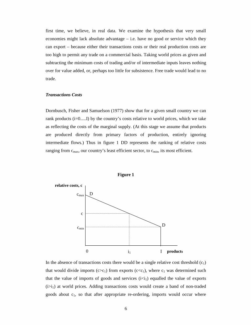
Dornbusch, Fisher and Samuelson (1977) show that for a given small country we can

rank products (i=0.....I) by the country’s costs relative to world prices, which we take

as reflecting the costs of the marginal supply. (At this stage we assume that products

are produced directly from primary factors of production, entirely ignoring

intermediate flows.) Thus in figure 1 DD represents the ranking of relative costs

ranging from cmax, our country’s least efficient sector, to cmin, its most efficient.

Figure 1

In the absence of transactions costs there would be a single relative cost threshold (c1)

that would divide imports (c>c1) from exports (c<c1), where c1 was determined such

that the value of imports of goods and services (i<i1) equalled the value of exports

(i>i1) at world prices. Adding transactions costs would create a band of non-traded

goods about c1, so that after appropriate re-ordering, imports would occur where

0 i1 I

relative costs, c

cmax

c

cmin

D

D

products

7

c>c1+tI and exports where c<cI-tE (where tI and tE are the cost of importing and

exporting respectively). Clearly the range (tI - tE) could be so large as to preclude

trade entirely.

In this world our country could remain trading in two ways. It could receive a non-

trading flow of foreign exchange – e.g. from accumulated assets, remittances or aid –

which permitted some imports in the absence of exports. Alternatively or additionally

it could receive prices for its exports above the world level – preferences – which

permitted exports despite its fundamental un-competitiveness. Both these cases

amount to living on rents. This might not be a problem if the rents were assured and

reliable, but if ever they dried up, very serious adjustment strains would be created. In

the limit, if local prices did not fall low enough to make cmin tradable at world prices

plus our economy’s transaction costs, life would become unsustainable.

It is sometimes argued that the ability to produce specific varieties of goods for niche

markets should allow very small countries to export effectively. While this is true to

an extent, it could still be insufficient to overcome the problems of high transactions

costs.

Real Costs of Production

The second example expands on the case that, with high trading costs, life might not

be sustainable. We locate it again in a simple Ricardian model of trade with constant

costs of production, but for simplicity, now with just two goods – cereals and bananas.

Let us assume that survival depends on consuming a given level of cereals but that our

country’s comparative advantage lies in bananas.

Imagine that the per capita production possibility frontier between cereals and

bananas is given by CB in figure 2, and that the minimal consumption of cereals

necessary for survival is S. In autarchy, this economy is unviable – its inhabitants

would starve - but if we allow international trade at the price ratio implied by AB, the

inhabitants can survive by selling bananas and buying cereals. Suppose that AB is the

ratio at which a large country can trade, but that a small country, which faces excess

trading costs, can realise fewer units of cereal per banana – say A’B. The small

8

country is now unviable – even with the advantages of trade: incomes are just too low.

It does not matter whether the excess costs reside in selling bananas or buying cereal,

or both. The important thing is that fewer units of cereal may be consumed per banana

produced.

Figure 2

The small country is still better off trading than not, just not sufficiently better off to

make life sustainable. Certainly it has no interest in curtailing trade. Note also that if

one wished to boost its income, either improving its productivity (i.e. pushing CB

out), or its terms of trade (rotating A’B clockwise towards AB) would suffice. Even

with given world prices, the latter could be achieved by lowering transactions costs or

by offering preferential access to a protected market. Conversely, removing such a

preference could push a viable economy below subsistence level.

Input Costs

The third model is grounded in the theories of effective rate of protection (ERP) and

domestic resource content (DRC), and takes as given that the production of goods for

the international market requires material inputs from that market. Taking all

international prices and input-output co-efficients as fixed, the value left over from

export sales for value added and non-traded inputs )~

( iV is:

∑−=Tj

jjiii papVε

~~~ (1)

B

cereals

S

A’

C

subsistence

A

bananas

9

)1()1(~

∑ +−−=Tj

jjjiiii tpatpVε

(1’)

where i, j count over products

ip~ are local prices

pi are world prices

ti are transaction costs

aij are input-output co-efficients, and

T is the set of traded inputs.7

The division between traded and non-traded inputs is very important here. Local

supplies will be used where they are cheaper than imported ones. For poor countries

the set for which this is true is likely to be small because poor technology and/or

scarce management resources frequently rule out local production. Similarly, for

small countries, the set will also be small because their scale is so limited. Moreover,

some products that have more or less to be non-traded nonetheless have to be

produced using traded inputs - e.g. electricity - so that high transactions costs and

small-scale compound each other. In short, the genuinely local input into

internationally traded goods, and thus the margin that can be squeezed to make

exports competitive, is likely to be small for poor and small countries. It is also plain

from equation (1’), and from past DRC exercises, that local value added can be

negative. In the DRC literature such observations lead to (justifiable) calls to correct

the policy distortions that cause this situation. Here, our starting point is the excess

costs faced by small and poor countries may be unavoidable and hence that very low

or negative value-added is also unavoidable – it reflects an inability to generate

acceptable incomes through trade. At best, all that the economies so afflicted might do

is generate autarchic subsistence incomes.

Clearly the assumption of fixed input-output co-efficient is too strong, so that

equation (1) may over-estimate the costs of smallness and remoteness. However, the

example illustrates the possibility that even with the best and most appropriate

technologies in the world, value-added could be small or negative.

10

2. The Approach

This section briefly presents our approach to testing the hypothesis that small

economies face serious cost disadvantages. We collect data on a wide range of the

costs of doing business across a series of differently sized economies8 and seek

regularities in the relationship between cost and size. Most of the costs are measured

in simply monetary terms, but we also collect information on some categorical

qualitative variables and on a few policy variables to see if policy varies

systematically with size. Since countries’ size varies only slowly, we rely on cross-

country variance to identify the size effect. Once we have estimated these cost

disadvantages, we weight them together, based on the cost structures of three key

industries, to create a single cost inflation factor for each product. We also calculate

what we refer to as income penalties for each industry. The income penalty reports by

how much value added is reduced in a small economy relative to an average sized one

if exports fetch only world prices while inputs face excess costs of smallness. The

industries selected are electronic assembly, clothing and tourism, as these are believed

to be the areas in which small remote economies have stronger competitive

advantages9.

We define size in terms of population – the traditional measure, see for example,

Kuznets (1960), Armstrong et al. (1998) and Easterly and Kraay (2000) – although for

some costs we also include GDP per capita (GDPpc) among our explanatory variables

so that there may be aggregate income effects too10.

Size is not the only feature of an economy that potentially affects its performance and

business costs. however. There are strong reasons for believing that location also

matters in terms of both who are your neighbours (e.g. Vamvakidis, 1998) and how

7 Note that the local returns for exportable production are world prices less the transactions cost, not the world price plus the tariff as we are used to from ERP analysis. 8 The sample of countries is given in annex 1. 9 Some studies (e.g. Armstrong et al., 1998) point to the positive correlation between services (e.g. tourism) and growth. Agriculture, however, is found to have a negative impact on growth. 10 Population is also better measured and more likely to be exogenous than GDP.

11

isolated you are from the main centres of economic activity (Redding and Venables,

2002a)11.

Unfortunately, size, region and insularity are highly collinear. As we can see in table

2, the Pacific and Caribbean regions are almost wholly comprised of small countries

and together comprise nearly the whole of our sample of small countries. Similarly,

these two regions provide practically all our island economies and contain very few

continental countries. Thus, smallness and insularity go very closely together.

Table 2: Sample Countries Cross-classified by Size, Region and Insularity

Population in Millions Region ≤0.4 0.4< ≤ 2 2 ≤<10 10< ≤50 >50 Pacific 11 2 1 - - Caribbean 8 3 1 - - Sub-Saharan Africa 1 5 2 10 1 Latin America - - 1 6 1 South Asia - - - 1 3 Rest Asia - - 2 2 5 OECD - - 7 11 8 Geographical Status Continental 1 6 13 30 18 Island 19 4 1

We try several different techniques to try to disentangle the locational effects

(remoteness and insularity) from the size effect. For example, we include a distance

variable for the cases where the data refer to links with specific main centres (e.g.

London or Tokyo), which is the case of transportation and communications (telephone

calls). Moreover, for sea transportation we include land distances to the port of

entry/exit and seek qualitative differences for cases where this exceeds a threshold or

where it involves crossing an international border. Isolation effects are explored by

the use of an island dummy in some relationships12.

Ultimately, however, we cannot clearly separate these two sets of effects, so we are

not able to assert with confidence which factor is responsible for the phenomena we

observe. The collinearities reflect a fundamental lack of information. Future

11 See Redding and Venables (2002b) for an overview. 12 See WM for a discussion of the definition of an island.

12

researchers might try to solve the problem by enlarging the sample (e.g. to collect data

for more islands and small economies outside the Pacific or Caribbean, to consider

more continental small countries such as Luxembourg, and to study islands within

countries to ascertain the costs of physical separation). For the present, however, our

only palliatives are theory and parsimony: exploiting theory to try to separate the

different effects and recognising the fundamental problem by not seeking too fine a

degree of explanation. Moreover, we would also plead that the policy problem is

essentially collinear: the main policy concerns are about what to do for economies that

are both small and remote.

3. The Business Cost Data

This paper is based on original business cost data for 92 economies, which were

assembled from four distinct sources. The largest contribution comes from the

Economist Intelligence Unit (EIU) which surveys 54 medium-sized and large

countries twice a year. The remaining surveys were commissioned by the

Commonwealth Secretariat for this study from regional organisations in various

(mostly small) economies: Imani Capricorn in Africa, The Caribbean Community in

the Caribbean and The Pacific Islands Forum in the Pacific. All these surveys date

from mid-2002. The survey instrument is given in WM13.

All survey data are subject to error and ours are no exception. Considerable effort was

required to interpret and clean them and in order to increase the value of the data we

have corrected the most obvious of the errors – for example, re-scaling prices that

have been reported in cents rather than dollars. See WM for details. Nonetheless a

number of difficulties remain, which we note very briefly as we come to them below.

We have two illustrations of the noisiness of the data. First, two African countries –

covered by Kenya and Zimbabwe – were both the EIU and the Imani samples.

Comparing the two sets of answers is salutary. For the questions requesting cardinal

answers the mean absolute proportionate difference between the two sources was

13

29.4% for Kenya (45 variables) and 56.8% for Zimbabwe (44 variables).14 Among the

categorical questions the corresponding statistic was 38.3% for Kenya and 10.0% for

Zimbabwe (10 variables each).15 In the areas of dispute, we have used the EIU data,

because we found them, on the whole, more plausible. The second area in which we

have two estimates of the same phenomenon concerns air freight costs from 5

Caribbean countries. The mean absolute difference of these data, is 69.8%!

Even after the first round of cleansing the data still contain a number of obvious

surprises and outliers. Where possible we confirmed unusual values from secondary

sources, but have over-ridden the reported values only in the most egregious of cases.

During the regression analysis outliers were sometimes identified in the form of

absolutely large residuals from our estimated relationships. Since our aim is to test the

relationship between the various business costs and size, we have in general

eliminated these from the regressions in order to preserve the normality of the

residuals and hence the legitimacy of the statistical inference. In all cases, however,

we report the direction in which the observation is outlying, and check that the nature

of the estimated relationship is not greatly changed by its elimination. If it is, we –

and our readers – should exercise great caution in drawing conclusions.

The variables used in the empirical study are given in annex 2 (continuous variables)

and annex 3 (categorical variables). The continuous variables are analysed by

regressing costs (in dollars) on the country’s size and other variables which we

believe might affect it and are reasonably readily available. All values are reported in

or converted to current US dollars and all refer to mid-2002. Regarding the

categorical variables, we estimate ordered logit equations for ranked data and binary

logits for the dichotomous data (more information is provided in the following

section). Although these categorical variables cannot be easily converted into dollars

13 It had been our intention to make these data available publicly, but the requisite permissions have not yet been received. 14 The statistic is the mean of )(*5.0/ 2121 zzzz +− where z1 and z2 are the two replies to the same

question from the two sources. 15 If the categories chosen by the two surveys for categorical variables were i1 and i2, we calculate the average of )1/()( 21 −− nii , where n is the number of categories, so that (n-1) is the maximum

difference.

14

and cents to compare with the monetary information, they help to inform us about the

qualitative advantages or disadvantages of size.

Complementary macroeconomic data were also necessary. The main source for GDP,

GDP PPP (Power Purchasing Parity) and Population was the World Development

Indicators 2002, although other sources were also used to complement this

information where necessary (Global Business Cost Survey and Asian Development

Bank). So too was information on air and sea distances. These came from

http://www.wcrl.ars.usda.gov/cec/java/lat-long.htm for great circle air distances and

SUDist (http://www.shipanalysis.com) for sea distances along recognised routes. See

WM for details.

4. The Regressions Models

This section describes our efforts to identify country-size effects in our costs data. The

main results are summarised in section 5 and further details can be found in WM. The

general approach was to fit log-linear models by Ordinary Least Squares between the

business cost variables and our measure of size (population), including also other

relevant regressors such as distance in the transportation cost equations. Where

appropriate we made allowances for insularity and for likely differences between high

and low-income countries. All equations were subject to a number of standard

diagnostics tests. Amongst others, we tested the normality of the residuals (Bera and

Jarque, 1981), functional form (RESET - including the squared prediction in the

equation – Ramsey, 1969) and heteroscedasticity (calculated from the regression of

the squared residuals on squared fitted values - Breusch and Pagan, 1981). We

responded to failures by trying a variety of different specifications (as long as these

made economic sense) and although we achieved improvements in some cases, there

were a few in which problems remained. For failures of normality, we simply

excluded the offending observations from the regression in order to render our

inferences more reliable (since most of them are valid only under the normal

distribution of residuals). We did check and report below, however, whether this had

material effects on the parameter estimates. Where heteroscedasticity persisted we

used White adjusted standard errors, in order to make out inferences more reliable and

15

in the few cases where we were able to remove functional from errors by re-

specifying the equation, we merely note the fact and pass on.

Our basic estimating equation for the continuous variables was

Ln (costs) = α0 + α1 Ln (Popn) + α2 [Ln(Popn)]2 + other variables

In the absence of any other theoretical guidance, our main motivations for using log-

linear models were the high dispersion of size (population and GDP) across our

sample, and the belief that size effects act roughly proportionally.

Turning to the other variables, for air freight costs we add distance measured by

great circle distances and in logarithmic form following Hummels (1999).

For sea freight costs we add the variable sea distances calculated from nautical tables

available from SUDist (http://www.shipanalysis.com). Where the principal economic

centre of a country is not the port we add in the internal land distances converted to

nautical miles. This procedure implies that land transportation costs are equal to

shipping costs (per mile), which is obviously not precisely true. Therefore, we also

include a dummy variable for all countries where the inland distances are greater than

a certain threshold. Amongst the different thresholds tested, 500 km seemed to give

the best results (L500). We also experimented with a dummy reporting the need to

cross an international land border, but it was never significant.

We excluded Australia (+) and Finland (-) from the sea-freight equations since, based

on their studentised residuals, they were huge outliers in all equations. And we also

added in an OECD dummy to solve persistent functional form problems: OECD

countries are arguably different from the rest of the sample in terms of infrastructure

and trading institutions (e.g., security), and therefore need to be isolated. The OECD

dummy is obviously a very crude indicator of such things but, here and elsewhere,

attempts to improve on it by using other variables to model infra-structure and

institutions directly are thwarted by the absence of such data for our very small

countries. Given that they are the focus of our study it seemed inappropriate to

exclude them wholesale from our estimation.

16

For each of the eleven wage variables the only additional variable is Ln(GDPpc),

which measures the living standards of the country, an obvious correlate of wages.

We also tried to include non-monetary benefits as stated in the Global Business Cost

Surveys, but these performed very poorly (perhaps because benefits can be either

complements or substitutes for money wages and the different effects cancel each

other out). We also observed that rich countries (OECD and the three Asian high-

income economies) have unusually high incomes compared with the rest of the

sample even after allowing for GDPpc. This may be due to their very different skills

levels, institutions and technologies. Thus, based on powerful graphical evidence –

see WM - we restricted the wages exercise just to developing countries.

We also tested for island effects in the wage equations since insularity can be an

obstacle to labour mobility. We define insularity as having fewer than 10 million

inhabitants and no significant land mass within a certain range, experimenting with

setting the range at 50, 500 and 1500 km. (The one exception was New Zealand due

to its degree of development.) However, since insularity and size are highly correlated

in our sample and insularity may have positive or negative effects on wages according

to whether it blocks inward or outward flows more effectively, we did not find these

variables useful.

The general specification used for utilities (telephone - except international calls -

water, electricity and fuel) included Ln(GDPpc), while for international telephone

calls we used the same specification as for air freight. For all utilities we test both

marginal costs (or something quite like it) and fixed costs (e.g. connection fees, etc).

Unfortunately we do not know the proportions of total cost that these two elements

account for and hence can not calculate the trade-off between them for a typical firm.

For the passenger travel costs we added Ln(GDPpc) to the airfreight specification to

account for different living standards (i.e., we would expect that people living in

England to travel more by plane than people in Zambia).

For the policy variables - various tax, subsidy and interest rates - we use a linear-log

specification since the policy variables are expressed as percentages, which are,

17

broadly speaking, scale free. In effect we are applying a log-log model to (1+x) where

x is the tax rate in question. These equations also include Ln(GDPpc).

For the categorical information on the frequency of disruptions, length of waits for

connection or repair we estimate size effects from Ordered Logit equations, since the

data can be ordered (i.e. it is better to have fewer disruptions than more). We thus

calculate the probability of a country falling into a particular class of disruption

according to its individual characteristics (e.g. income and size) as:

Prob(country i is in class j) = exp (μj + β’xi)

λ∑

exp(μλ+ β’xi)

where β’xi = α1Ln(GDPpc) i + α2*Ln(Pop)i

The inclusion of GDPpc captures the different living standards, and given that higher

numbered classes entail worse service (more disruptions, longer waits) we expect it to

have a negative sign.

5. The Regression Results

The main results are summarised in table 3. This reports, in column order: the

regression co-efficients on population and population squared, the joint test of their

significance, the co-efficients on distance, GDPpc, an inland transportation dummy,

and the OECD dummy, R2 and the number of observations. Following these are the

statistical tests: for heteroscedasticity (Het - where x denotes failure – i.e. the presence

of heteroscedasticity); for functional form (FF - x denotes failure); the number of

observations dropped to achieve normality, distinguishing those for which size and

the target variable are both above or below their respective means (+) from those with

one above and one below (-)16; and the number of zeros in the dependent variable.

Finally come the cost disadvantages implied by the equations for four example

16 This distinction is between omissions that will tend to increase the slope of the cost-size relationship (+) and those that will reduce it.

18

countries (those in italics are based on statistically insignificant estimates, while

where we think there is no evidence of size effects we write 0).

The cost disadvantage ratios summarise the costs of smallness by presenting, for four

representative countries, the percentage excess costs of their inputs relative to those of

the median country. The exemplar countries are located 4th, 18th , 29th and 36th in our

ranking by size, expressing their percentage disadvantage relative to our median

country, ranked 46th. To make the examples concrete, they correspond to our

populations of

Micro economies Anguilla 12.13 thousand Very small Vanuatu 197 thousand Threshold Botswana 1,602 thousand Small Singapore 4,018 thousand Median Hungary 10,022 thousand

The so-called ‘threshold’ corresponds roughly to the population threshold of 1.5

million used in the report Small States: Meeting Challenges In The Global Economy

(April 2000) prepared by the Commonwealth Secretariat / World Bank Joint Task

Force on Small States and subsequently elsewhere (e.g., Jansen, 2004). We include it

and one larger exemplar in the table to test whether the disadvantages of small scale

really have become negligible by this size.

The estimates for airfreight costs suggest that there are significant size effects for

outward transportation (as shown by the joint significance F-tests in column 3). The

negative sign on population and positive sign on the squared term implies a u-shaped

relationship between population and costs. The turning points vary between 1.5

million inhabitants and 3.5 million inhabitants (for the outward regressions), which

leaves at least 30 small economies on the downward part of the curve. These estimates

are robust to the exclusion of certain observations (to solve normality problems) and

also to tests of asymmetries between the two arms of the 'U’ and the omission of very

large countries. Distance is always significant at 1%, with coefficients varying from

0.248 to 0.533, but the R-squares are relatively low (0.09 to 0.36).

19

Tab

le 3

: Su

mm

ary

of t

he S

ize

Reg

ress

ions

for

Con

tinu

ous

Var

iabl

es

Nor

m.

Cos

t di

sadv

anta

ges

Reg

ress

ion

Ln(

Pop

) [L

n(P

op)]

2 F

-tes

t (P

op)

Ln(

Dis

tanc

e)

Ln(

GD

Ppc

) L

500

OE

CD

R

-Sq.

O

bs.

Het

. F

.F.

- +

Log

Z

eros

M

icro

V

. Sm

all

Thr

esho

ld

Sm

all

To

Lon

don

-0.2

81**

0.

018*

* 2.

565*

0.

248*

**

- -

- 0.

19

91

60

.3

8.2

-3.2

-3

.1

Fro

m L

ondo

n -0

.189

0.

010

0.77

0 0.

369*

**

- -

- 0.

23

83

62

.1

18.9

4.

3 1.

3 T

o T

okyo

-0

.326

***

0.02

0***

4.

007*

* 0.

336*

**

- -

- 0.

14

84

3

85

.3

15.2

-1

.1

-2.2

F

rom

Tok

yo

-0.0

57

0.00

4 0.

469

0.37

2***

-

- -

0.09

80

x

3

7.1

-0.4

-1

.7

-1.2

T

o N

Y

-0.2

78**

* 0.

019*

**

5.17

9***

0.

499*

**

- -

- 0.

36

84

1 3

45

.2

1.0

-6.6

-4

.9

Air

frei

ght

Fro

m N

Y

-0.2

11

0.01

4 0.

886

0.53

3***

-

- -

0.17

82

37.2

3.

2 -3

.8

-3.1

T

o R

otte

rd.

-0.2

90**

* 0.

011*

16

.601

***

0.21

8***

-

0.41

9**

-0.3

55**

0.

61

70

19

5.3

67.0

21

.8

9.3

Fro

m R

otte

rd.

-0.3

07**

0.

009

29.2

68**

* 0.

135*

-

0.72

7***

-0

.416

**

0.70

62

287.

4 10

0.1

33.5

14

.6

To

Yok

oh.

-0.4

06**

* 0.

017*

* 29

.450

***

0.54

8***

-

0.31

0**

-0.2

91**

0.

60

78

30

1.5

87.2

25

.5

10.4

F

rom

Yok

oh.

-0.3

16**

0.

011

24.9

73**

* 0.

678*

**

- 0.

126

-0.3

57**

* 0.

64

75

25

1.6

85.0

27

.7

11.9

T

o N

Y

-0.3

11**

0.

015*

* 5.

819*

**

0.20

2**

- -0

.131

-0

.177

0.

29

75

x

14

8.3

44.4

4.

5 4.

5

Sea

frei

ght

Fro

m N

Y

-0.3

02**

0.

015*

* 11

.303

***

0.04

8 -

0.11

1 -0

.378

* 0.

22

75

x

13

3.7

39.4

10

.2

3.7

CW

-0

.075

***

- -

- 0.

525*

**

- -

0.67

63

65.5

34

.3

14.7

7.

1 C

O

-0.0

54**

* -

- -

0.48

9***

-

- 0.

67

63

x

43

.7

23.6

10

.4

5.1

KP

-0

.080

***

- -

- 0.

452*

**

- -

0.76

63

71.1

36

.9

15.8

7.

6 B

CL

-0

.050

* -

- -

0.25

7***

-

- 0.

39

58

39

.9

21.7

9.

6 4.

7 B

CF

-0.0

40

- -

- 0.

229*

**

- -

0.29

59

30.8

17

.0

7.6

3.7

GM

-0

.060

**

- -

- 0.

461*

**

- -

0.63

63

49.6

26

.6

11.6

5.

6 P

C

-0.0

12

- -

- 0.

543*

**

- -

0.60

63

8.4

4.8

2.2

1.1

QT

-0

.047

**

- -

- 0.

532*

**

- -

0.73

63

37.1

20

.3

9.0

4.4

BM

L

-0.0

64**

-

- -

0.29

8***

-

- 0.

35

58

x

53

.7

28.6

12

.5

6.0

BM

F -0

.046

-

- -

0.29

1***

-

- 0.

26

58

36

.2

19.8

8.

8 4.

3

Wag

es

GR

N

-0.0

71**

* -

- -

0.51

5***

-

- 0.

73

61

1 1

61

.1

32.2

13

.9

6.7

Lon

don

-0.1

01**

* -

- 0.

418*

**

-0.2

27**

* -

- 0.

61

89

1

97

.1

48.7

20

.3

9.7

Tok

yo

-0.1

17**

* -

- 0.

001

-0.1

96**

* -

- 0.

36

89

11

9.4

58.4

23

.9

11.3

N

Y

-0.1

52**

* -

- 0.

169

-0.3

93**

* -

- 0.

61

90

x

17

7.6

81.7

32

.1

14.9

L

ocal

-0

.073

* -

- -

-0.0

74

- -

0.05

81

5

0.0

0.0

0.0

0.0

Ins

t. Fe

e 0.

058*

-

- -

0.10

6 -

- 0.

06

90

1 -3

2.3

-20.

4 -1

0.1

-5.2

Tel

epho

ne

Lin

e R

ent.

-0.0

26

- -

- 0.

364*

**

- -

0.42

88

2

19.1

10

.8

4.9

2.4

Usa

ge

-0.0

98**

* -

- -

-0.0

21

- -

0.19

84

1

2 1

93.1

47

.0

19.7

9.

4 E

lect

rici

ty

Con

nect

. 0.

103

- -

- -0

.223

-

- 0.

07

67

9 0.

0 0.

0 0.

0 0.

0 U

sage

-0

.184

***

- -

- 0.

024

- -

0.14

82

2 4

0.0

0.0

0.0

0.0

Wat

er

Con

nect

. 0.

219*

**

- -

- 0.

409*

**

- -

0.35

63

2

1 11

-7

7.0

-57.

7 -3

3.1

-18.

1 D

iese

l -0

.084

***

- -

- -0

.110

**

- -

0.32

62

1

75.8

39

.1

16.7

8.

0 F

uel

Pet

rol

-0.0

41**

-

- -

-0.0

25

- -

0.11

61

1

1

31.7

17

.5

7.8

3.8

Lon

don

-0.1

16**

* -

- 0.

641*

**

-0.1

60**

* -

- 0.

93

86

x

3

11

8.0

57.7

23

.7

11.2

T

okyo

-0

.106

***

- -

0.45

5***

-0

.285

***

- -

0.58

88

103.

8 51

.7

21.5

10

.2

P. T

rave

l N

Y

-0.1

21**

* -

- 0.

871*

**

-0.2

13**

* -

- 0.

76

87

x

1

12

5.4

60.9

24

.8

11.7

O

ffic

e -0

.399

0.

035*

* 16

.349

***

- 0.

729*

**

- -

0.51

86

x

2

-7.0

-3

4.4

-28.

3 -1

7.8

Lan

d F

acto

ry

0.04

0 -

- -

0.25

6***

-

- 0.

29

73

x

8 8

0.

0 0.

0 0.

0 0.

0 L

endi

ng

1.56

1**

-0.1

07**

5.

812*

-

-2.6

30**

* -

- 0.

50

82

x

1 7

-2

.1

0.0

0.4

0.3

Ban

k D

epos

it

0.32

2***

-

- -

-1.0

78**

* -

- 0.

29

83

x

1 5

-2

.2

-1.3

-0

.6

-0.3

R

esid

ents

0.

373

- -

- -0

.091

-

- 0.

03

84

1 6

-2

.5

-1.5

-0

.7

-0.3

C

orp.

Tax

N

on-R

esid

ents

0.

113

- -

- -0

.767

* -

- 0.

04

84

6

-0

.8

-0.4

-0

.2

-0.1

W

eigh

ted

-0.1

93

- -

- -3

.492

***

- -

0.47

51

x

3

2

1.3

0.8

0.4

0.2

Un-

Wei

ghte

d -0

.057

-

- -

-3.6

23**

* -

- 0.

58

47

x

3

0.

4 0.

2 0.

1 0.

1 I

mp.

Dut

ies

% R

even

ue

-6.0

51**

* -

- -

-7.0

28**

* -

- 0.

55

65

x

40

.6

23.8

11

.1

5.5

20

Legend to Table 3 Obs. - Refers to the number of observations used in the final regressions. In italic are the regressions where OECD and the 3 high-income Asian countries were excluded. F-test - Joint significance test on the coefficients of Ln(Pop) and [Ln(Pop)]2. In the regressions with heteroscedasticity this is actually a Wald-test (with White-adjusted errors). Het. - x denotes regressions which have White-adjusted standard errors to overcome the remaining Heteroscedasticity F. F. - x denotes regressions which fail the Functional Form test (RESET) Norm. - States the number of observations excluded due to normality problems. '+' represents the number of observations that would have a positive effect on the slope and '-' the opposite. I.e. the ‘+’ refers to cases where (x-μ)(s-σ) >0, where x is the LHS variable, s Size and μ and σ their respective means. We did not recalculate the mean size for every different sub-sample, but used the mean of the whole sample and the mean excluding the high income counties as appropriate. Geometric mean (all sample) - 4563.1 thousand inhabitants Geometric mean (63 Obs.) - 2342.8 thousand inhabitants Log Zeros - Indicates the number of observations that stated '0'. These were excluded since zeros cannot be logged. In italics we put the cases where these exclusions may affect our general conclusion about the results. Cost disadvantages - These are based on the ratio between the costs of each of the 4 exemplar countries (chosen to represent different population categories) and the median country. For the cost regressions these represent % deviations from a fictional median country with around 10 million inhabitants. For the policy variables, these disadvantages are actually expressed in percent points. The cases where the evidence of a population effect is insignificant by different from zero are in italics. The zeros are cases where there is no convincing case for cost disadvantages (based on the significance of the population effects and sensitivity tests undertaken to assess the impact of the exclusions of the '0' observations). * Significance at 10% ** Significance at 5% *** Significance at 1%

Wages CW - Construction Worker CO - Checkout Operator KP - Kitchen Porter BCL - Bank Clerk/Teller in Local Bank BCF- Bank Clerk/Teller in Foreign Bank GM - Garage Mechanic

PC - Payroll Clerk QT - Qualified Teacher BML - Bank Manager in Local Bank BMF- Bank Manager in Foreign Bank GRN - General Registered Nurse

21

A surprise is the apparent absence of significant size effects in the inbound freight

rates (from London etc). Inbound rates are generally significantly higher than

outbound ones, and we speculate that the difference arises because of different

practices in consolidating consignments. Outbound, export agents seek to consolidate

and so are able to do something to overcome the disadvantages of small size. This is

feasible for outbound journeys because exports are not highly diversified and stem

from a small number of economic entities. Inbound, on the other hand, the co-

ordination problems are greater, with greater diversity of goods, entities and origins

and also great distance between national agents at home and the place where

consolidation must be done (i.e. in the partner country).

Turning to sea freight costs, we can see that there are strong size effects for all

regressions: the coefficients on population are always significantly negative and the

joint significance of the population variables very high. In this case the ‘U’ is much

steeper and the turning points much higher: in two cases they are far beyond any

existing country’s size. That is, sea freight shows much higher minimum efficient

scale than airfreight. (We decided to keep the two insignificant squared terms to

maintain the same functional form for all sea freight regressions.)

As expected, the land transportation dummy, L500, takes a positive sign (except ‘to

NY’ where it is not significant) and is significant in three cases. One would expect

that the magnitudes of the inland dummy would not change greatly over the three

partner ports since the cost of transporting a FCL from, say, Kampala to Mombassa

would be the same irrespective the final destination, and also the same as Mombassa

to Kampala. The difference in samples across partners may explain why this is not

apparent in our results. The OECD dummy always assumes a negative sign and is

significant in five of the six cases. As explained above, we see it as reflecting different

infrastructures and institutions in these countries. Distance is almost always

significant (the exception is ‘from NY’). The R-squares are much higher than for

airfreight for Rotterdam and Yokohama, although not for NY17. Only one of the

regressions presented functional form problems – see column headed FF in table 3.

17 The New York regressions are altogether less convincing. But we do not know why.

22

The samples for the nominal wage regressions exclude the OECD and the three high-

income Asian countries. This decision followed a careful examination of data plots

that displayed very great differences between the rich and poor sub-samples. Among

developing countries the relationship between size and wages is log linear (since none

of the squared terms for population was statistically significant). GDPpc is always

positive and significant at 1%, with coefficients varying from 0.229 and 0.298 for

bank related jobs and from 0.452 and 0.543 for the rest. Coincidently, the regressions

for bank clerks and bank managers had significantly lower R-squares than the rest, a

fact which we attribute to the multinationality of the sector. Inter-country comparisons

are much easier within a company than between companies, and so the relationship of

the wage with national variables is more readily ‘contaminated’ by spillovers between

branches. Population is significant in 8 of the 11 wage regressions (7 at 5%) with the

elasticities ranging from -0.047 to -0.080; all eleven regressions suggest a negative

relationship between size and wages. The fact that two out of the three non-significant

size effects refer to foreign banks (bank clerk and bank manager) again, we believe,

reflects multinationality. There is no suggestion of functional form problems, and we

had to deal with outliers in only one of the regressions.

Nominal wages may be higher in small countries because the cost of living is higher

for precisely the sort of reasons we are discussing in this paper. To explore this we

also included the PPP adjustment factor in the equation to capture ‘real’ price

differences. This is strongly correlated with size and absorbed some of the size

effects. However, all the population effects remained negative and three remained

significantly different from zero. Once we allow for the negative relationship between

population and the PPP factor, the net effect of population on wages is almost

identical whether we break out the ‘real’ price effects or not.

For utilities we ran regressions for both fixed and variable costs. The main problem

faced with the utilities was the high number of zeros reported. Since our log-linear

regressions are potentially highly sensitive to these, we must be very careful with the

interpretation of the results, and apply sensitivity tests to assess the importance of

dropping these observations.

23

For international telephone costs, population is always significantly negative at 1%

(from -0.101 to -0.152). But distance does not seem to be an important determinant of

costs, except ‘to London’. As for virtually all utilities’ marginal costs, the coefficients

on GDPpc are robustly negative, indicating that people in richer countries pay less

than those in poorer countries. The estimates for local telephone costs are much

weaker. Although in table 3 the population effect is significant (at 10%) and negative,

our sensitivity tests suggest that if we had included the five recorded zeros, this would

not persist18. Thus we decided that we could not identify convincing cost

disadvantages for this variable and record O in the cost disadvantage column. In

addition, GDPpc was not significant and the R-squared very low (0.05).

Turning to the fixed costs of telephones, installation fees proved to have a weak but

positive relationship with size (at 10%), although GDPpc was not significant and the

R-squared was low. In this case the ‘zeros’ would reinforce this result, so we conclude

that installation fees do tend to be higher in larger countries. Finally, for line rental

fees, we found that GDPpc has a strong impact, but that population is not a significant

determinant (although the estimate suggests a negative relationship between size and

line rental costs).

The results for electricity marginal costs seem pretty robust even though we had to

exclude three anomalous observations and one ‘zero’19. The population coefficient is

significantly negative at 1% and the R-square equals 0.19. We cannot prove the

existence of a relationship between size and electricity connection costs however,

although the co-efficient suggests a positive relationship. There were nine zeros (for

countries ranging from Nauru and Senegal to Sweden and Australia), and different

ways of treating them gave different results.

Turning to water, we find a negative relationship between size and usage costs

(significant at 1%), while GDPpc was not significant and the R-squared was 0.14.

However, again the zeros look influential so we decided not to include these results in

18 We conclude this first, by observing whether the zeros refer to large or small countries and thus whether, ceteris paribus, they reinforce or undermine the reported signs. Second, we re-estimate the equation replacing the zeros by a fraction of the smallest non-zero value in the sample. 19 Czech Rep. ($1.4 per kilowatt) Mauritius ($2.08) and Nigeria ($2.70), compared with $0.22 in the most expensive OECD countries – Poland/Mexico

24

the cost disadvantage exercise. For water connection fees, we found a positive size

effect on the regression. GDPpc was also significant at 1%. The 11 zeros would

probably attenuate this result since most of these are for large countries. Nevertheless,

to be conservative we do carry these estimates forward.

In the fuel regressions, we again had to exclude the OECD and 3 high-income Asian

countries based on various data plots. The results illustrate a negative significant

relationship between size and the cost of fuel (-0.084 for diesel and -0.041 for petrol).

However, GDPpc is significant only for the diesel regression, where the R-squared is

substantially higher compared to the other.

The exercise on passenger travel used data provided by the Commonwealth

Secretariat’s travel agents. The results are pretty much consistent across the three

different destinations. The elasticity with respect to the population varies from -0.106

to -0.121, while that on GDPpc negative (varying from -0.160 and -0.284) and that on

distance positive. All coefficients are significant at 1% and the R-squares are high.

Two regressions seem to fail the functional form test (RESET), however, and since

the inclusion of a squared term (either on population or distance) proved to be

insufficient to cure the problem, we have had to live with it.

The last of the standard regressions was on land rents. Here we had severe problems

with missing observations and outliers. We managed to estimate a relationship for the

costs of office space, but the same was not possible for factory space. For office

space, the population variables are jointly significant, but since the coefficient on

population is small (and insignificant) the turning point occurs very early. Hence the

predominant relationship between size and office costs is positive. For factory rentals,

we were unable to find a significant relationship with size, especially given the

numerous outliers in the sample. The estimates, however, suggest again a positive

relationship. At first sight these results might look as if they show advantages to being

small. However, the Ricardian theory of rents suggests that land rents reflect the

surplus between earnings and costs, and hence that low rents merely serve to confirm

the disadvantages of small size seen above.

25

Table 4: Estimates for the Ordered Logit Equations on Categorical Variables

Regression Ln(Pop) Ln(GDPpc) Cat=1/2

pop ('000) Cat=2/3

pop ('000) McFadden’s Pseudo-R2

Obs.

Un-Skilled -0.169* 1.0*** 340.8078 0.7730 0.2 92 Semi-Skilled -0.361*** 0.4** 1892.8546 3.7076 0.1 92

Workers’ Availability

Skilled -0.392*** -0.3** 15803.2397 55.1362 0.1 92 Connection -0.064 -0.6*** - - 0.1 92 Disruption -0.176** -0.8*** 9169.5955 0.0003 0.2 92 Telephone Repair -0.098 -0.4** - - 0.1 92 Connection -0.021 -0.5*** - - 0.0 91

Electricity Disruption -0.242*** -1.1*** 56832.1320 1.4408 0.2 92 Connection 0.055 -0.4*** - - 0.0 90

Water Disruption -0.271*** -1.0*** 3205.8005 0.3942 0.2 91

Obs: Cat = 1 and Cat = 2 are based on a GDPpc = $10,000

For the categorical variables we estimate ordered logit equations to explore the

relationships between size (population) and the different categories of disruption or

waiting time. Table 4 reports the results. For each issue it reports the co-efficients on

population and GDPpc, the population thresholds between categories 1 and 2 and

between categories 2 and 3 assuming a GDPpc of $10,000, McFadden’s Pseudo-R2 as

a measure of fit and the number of observations used20.

We start with availability of workers. We ran regressions relating the availability of

each of three types of workers (unskilled, semiskilled and skilled) to size (logged

population) and (logged) GDPpc. Although, as we would expect, we do not have

strong evidence for unskilled workers, for semiskilled and skilled workers there are

obvious reported shortages in small countries. The minus sign attached to the

population coefficient represents the greater dependence of small economies on the

import of semiskilled and skilled labour (lower categories mean less need to import

workers from abroad). It is comforting to note the GDPpc effects suggest that richer

countries lack unskilled workers, and semiskilled workers to a lesser extent

(evidenced by a positive sign in GDPpc), but relatively speaking, have an abundance

of skilled workers. The thresholds between categories 1 and 2 are 1.8 and 15.8 million

respectively for semi skilled and skilled workers, which suggests that a large range of

countries are small enough to face shortages of skills, especially since the thresholds

are evaluated at $10,000pc and the skills shortages will be greater at lower incomes.

20 The population thresholds report the sizes at which a country with GDPpc of $10,000 would be predicted from category 1 (no problems) to category 2 and from 2 to 3.

26

For telephone, while there were no significant size effects for connection and repair

times, there was evidence that disruptions tend to occur more frequently in small

countries. This conclusion is repeated precisely for water and electricity. For quite

understandable reasons, small countries are more vulnerable to utilities disruptions

than are larger countries21.

The second substantive question to address is whether policy varies with the size of

countries. This might occur, for example, because small societies are easier or harder

to govern, or if the costs of implementing particular policies are not proportional to

size. We used linear-log regressions for the policy variables, since the policy variables

are measured in percentages. There were severe problems with outliers in almost all

of these regressions, but some tentative conclusions can be drawn. There appear to be

significant relationships between country size and bank lending and bank deposit

rates, linear for the latter and non-linear for the former (table 3). Thus, small countries

appear to have lower deposit rates than the median country, but for lending rates we

can say that only for very small countries22. The effect of GDPpc is significantly

negative in both equations, meaning that high per capita income countries have lower

interest rates.

With reference to corporate tax, we could not establish a convincing relationship

between either size or GDPpc and the tax rate. Thus, although we are clearly not

capturing much of the explanation of tax rates (see the very low R-squares), the

results certainly do not suggest that small countries tax more23.

The final block on table 3 concerns import duties. Although we find strongly

significant coefficients for GDPpc, we were unable to establish a convincing

relationship between size and import duty rates (weighted and un-weighted): the

negative sign suggests that small countries tend to have higher import duties, but with

t-statistics well below unity, this is not at all significant statistically. On the other

21 In WM we also present cross tabulations of disruption and waiting times by size class. They confirm these results. 22 Because the relationships are linear-log the disadvantage ratios are expressed in percentage points not percentage terms. 23 For an in depth study of size and taxation see Codrington (1989).

27

hand, receipts from import duties as a percentage of tax revenue did prove to be

robustly and significantly higher in small countries. GDPpc was also negative and

significant at 1%, confirming that in richer countries import duties provide a smaller

share of total tax revenue. The relationship with size seems intuitively plausible, for in

small economies very large shares of consumption are imported (increasing the

numerator and reducing the denominator of the fraction to be explained). Indeed, in

the limit, if imported inputs into industry are exempted, as they frequently are, import

duties become very similar to consumption taxes and thus probably rather efficient

sources of revenue.

Finally, we have dichotomous data on three policy variables – the existence of special

interest rates or tax incentives for exporters, and the existence of export duties.

Testing (through binary logits) for differences in the sizes of the economies that

display these features and those that do not, we find that small economies are less

likely to give tax incentives or have special interest rates for exports.

We did also collect information on general indirect tax rates and budget deficits, but,

unfortunately, neither set was usable – the former because the quoted ranges were too

large (e.g. 0-350% for Brazil) and the latter because the survey did not specify

whether to include a minus sign on the deficit, and practice evidently varied across

correspondents.

6. The Disadvantages of Smallness: Cost Inflation Factors and Income Penalties

Tables 3 and 4 leave a strong impression of the excess input costs arising from small

size, especially for micro and very small economies. However, we still need to

confirm that these excess costs add up to a material competitive disadvantage on the

world market. To do this we estimate the cost structures of three export industries

typical of developing countries – electronic assembly, clothing manufacture and

hotels and tourism – and use them to weight together the cost disadvantages above to

create a single cost inflation factor for each product.

28

The cost structures are based on the input-output tables from the GTAP consortium.

For each industry we collapsed the input structure into three primary factors – skilled

and unskilled labour and capital – and about a dozen intermediates. We then arrayed

the (value) input shares across the sixty-five countries for which data were provided

(there is considerable variance) and tried to infer the likely shares for the median sized

developing country. The valuation is at producer prices – i.e. essentially the same

basis as our collected cost data – and so the shares provide the weights required for

creating base weighted indices of the cost disadvantages relative to the median in the

exemplar economies.

That is, writing Cij for the percentage cost disadvantage factor for input i in exemplar

country j, measured relative to the median, we seek to infer the weights Wi of each

input in total inputs in the median country. Thus the cost inflation factor for exemplar

country j, Cj,

Cj = Σ Wi Cij

i

is a base-weighted index of excess costs. If the weights can be systematically varied

across countries to reduce the (value) shares of relatively expensive inputs, the Cj will

exaggerate the cost disadvantages. But given the relatively broad classes of inputs we

deal with, this does not seem likely to be a major problem.

To create the indices we need to distil the results in the last four columns of table 3

into a single figure for each identified input. In general we use the averages of the

figures in that table and further weight them together using crude a priori weights.

Whenever a cost disadvantage is not statistically significant in the table, we assume

the value to be zero here. We took averages of outbound and inbound transport costs

separately for exports and imports respectively (weighting airfreight one-third and

sea-freight two-thirds). For skilled labour we used the cost disadvantage for skilled

labour above, and for ‘Unskilled Labour’ the weighted average of our original results

for unskilled and semi-skilled (one-third for semi-skilled and two-thirds for

unskilled). This fits reasonably well with the GTAP definitions of skills. Finally, for

the cost of utilities we consider the averages only for the marginal cost component,

29

ignoring the connection fee (which means that we over-state the costs of smallness)

and the costs of disruption (which means that we understate them).

Second, we need to determine what proportion of the cost of each input is exposed to

the disadvantage factors. We distinguish five different treatments:

• Internationally traded intermediates are assumed to be available at the price of the

median country plus the excess transport costs identified above assuming that 8%

of the gross value of these goods is accounted for by international transport. Thus

for the smallest countries, for example, inputs of textiles into clothing account for

37.5% of cost, and face a premium of 150% on 8% of their value. This adds 4.5%

to the cost of clothing exports. We apply the same disadvantage factors to the full

value of small economies’ exports of electronics and clothing.

• Inputs of labour bear their own cost disadvantage factors and we assume that the

same factors apply to inputs of essentially non-tradable services. (We make no

allowances for other inefficiencies deriving from small size in these sectors.) For

the tradable component of services categories we assume that foreign competition

imposes some discipline (or displacement), and hence we halve the labour

disadvantage factors when applying them to each service in aggregate. We make

no further allowances for the labour availability disadvantages identified above.

• For capital our measured cost disadvantage factors – bank lending rates - are not

very appropriate. We assume conservatively that capital costs are 15%, 10%, 5%

and 5% above median values for our four exemplar small economies respectively.

These excesses essentially reflect investors’ ignorance of small economies and the

greater variability that the latter, almost inevitably, face. These factors are not

large: if the cost of capital is 10% in the median country we make it 11.5%, 11%,

10.5 and 10.5% for four exemplar countries respectively.

• For utilities we use the cost disadvantage factors from the table directly. As we

noted above, we ignore both the connection fees and the excess disruptions that

small economies face.

• Finally, for exports of tourism we assume that visitors have to pay the excess costs

of personal travel identified in the table and that these account for 25% of the

30

costs of a visit. Hence for recreation we have an exposure factor of 25% and a cost

disadvantage factor of 116% for the smallest economies24.

Table 5 summarises the cost disadvantage information that we use in our subsequent

calculations on clothing. It reports our estimates of (a) the cost shares of each input,

(b) the assumed exposure to the disadvantage factors, and (c) the summary

disadvantage factors for each input for each of our four exemplar small countries.

Table 5: Cost structures for Clothing and Cost Disadvantage Ratios

Cost Disadvantage Factors (%)

Central Estimate

(%)

Share subject to inflation Micro V. Small Thresh. Small

Comment

Unskilled Labour 15 1 47.5 25.1 10.9 5.3 UnSkilled & SemiSkilled Skilled Labour 2.5 1 38.0 20.3 8.9 4.3 Skilled Capital 13 1 15.0 10.0 5.0 5.0 Textiles 37.5 0.08 149.5 49.9 15.9 6.7 Av. Import - Transport WearingApp 4 0.08 149.5 49.9 15.9 6.7 Av. Import - Transport LeatherProd 1.25 0.08 149.5 49.9 15.9 6.7 Av. Import - Transport Energy 1.25 1 73.4 37.7 16.0 7.7 Electricity and Fuel MachEquip 1.75 0.08 149.5 49.9 15.9 6.7 Av. Import - Transport ChemRubPlast 3.25 0.08 149.5 49.9 15.9 6.7 Av. Import - Transport Trade 7 1 22.2 11.7 5.1 2.5 Labour*0.5 Transport 2 1 157.0 48.4 13.1 5.5 Airfreight & Seafreight Communication 0.5 1 98.5 47.2 19.1 9.0 Telephone FinBusServ 4.5 0.5 22.2 11.7 5.1 2.5 Labour*0.5 OtherGoods 4 0.08 149.5 49.9 15.9 6.7 Av. Import - Transport OtherServics 2.5 0.5 22.2 11.7 5.1 2.5 Labour*0.5 export transport factor 0.08 164.6 46.8 10.3 4.2 Av. Export - Transport

The next step is to calculate the income penalties that these costs disadvantage factors

generate. Supposing that exports must be delivered at the same price as the median

country would charge, the excess costs will decrease the returns of economic activity

in small countries. The degree by which these will be reduced will depend on which

costs are unavoidably inflated and which returns can be squeezed to restore

competitiveness. Dividing inputs into endogenously and exogenously priced sets, and

using T for the latter, we calculate

24 In retrospect we accept that these factors may be a bit large, given that most tourists travel on package holidays, which helps agents avoid the costs of small consignments.

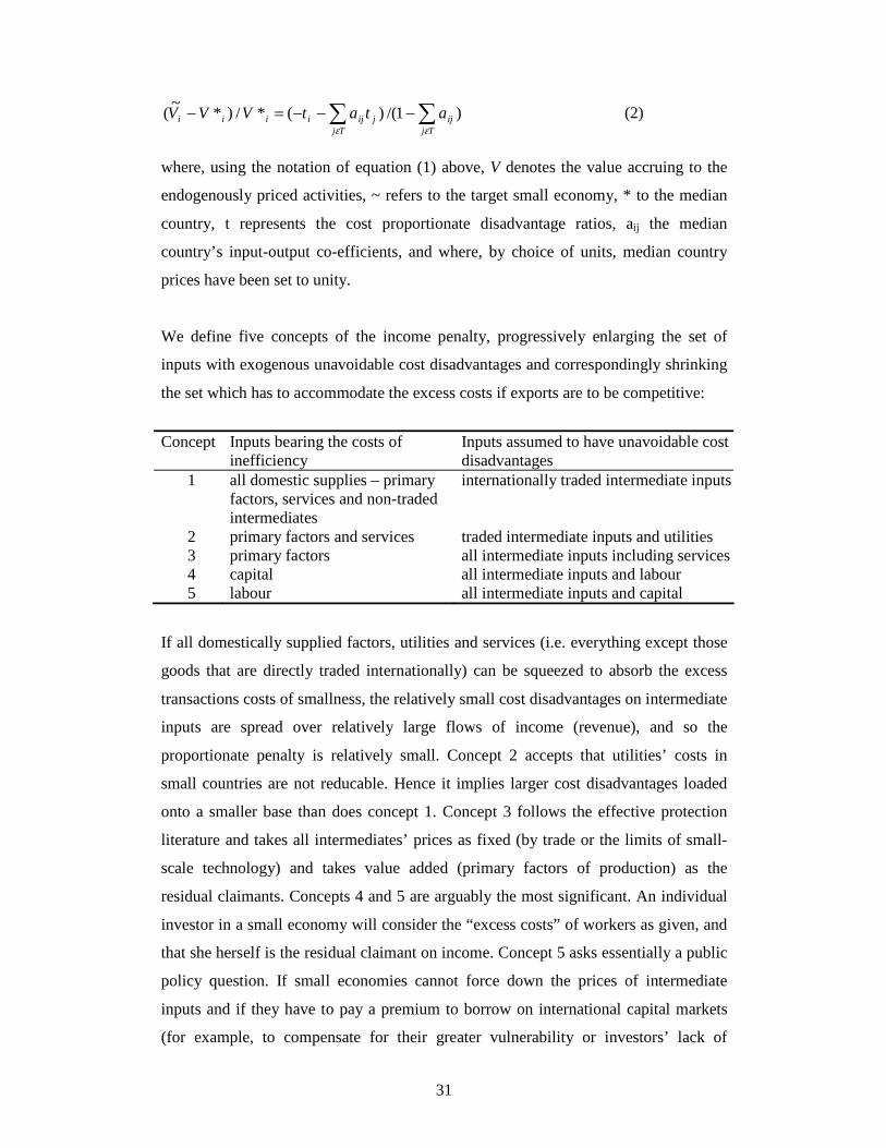
31

∑∑ −−−=−Tj

ijTj

jijiiii atatVVVεε

)1/()(*/)*~

( (2)

where, using the notation of equation (1) above, V denotes the value accruing to the

endogenously priced activities, ~ refers to the target small economy, * to the median

country, t represents the cost proportionate disadvantage ratios, aij the median

country’s input-output co-efficients, and where, by choice of units, median country

prices have been set to unity.

We define five concepts of the income penalty, progressively enlarging the set of

inputs with exogenous unavoidable cost disadvantages and correspondingly shrinking

the set which has to accommodate the excess costs if exports are to be competitive:

Concept Inputs bearing the costs of

inefficiency Inputs assumed to have unavoidable cost disadvantages

1 all domestic supplies – primary factors, services and non-traded intermediates

internationally traded intermediate inputs

2 primary factors and services traded intermediate inputs and utilities 3 primary factors all intermediate inputs including services 4 capital all intermediate inputs and labour 5 labour all intermediate inputs and capital

If all domestically supplied factors, utilities and services (i.e. everything except those

goods that are directly traded internationally) can be squeezed to absorb the excess

transactions costs of smallness, the relatively small cost disadvantages on intermediate

inputs are spread over relatively large flows of income (revenue), and so the

proportionate penalty is relatively small. Concept 2 accepts that utilities’ costs in

small countries are not reducable. Hence it implies larger cost disadvantages loaded

onto a smaller base than does concept 1. Concept 3 follows the effective protection

literature and takes all intermediates’ prices as fixed (by trade or the limits of small-

scale technology) and takes value added (primary factors of production) as the

residual claimants. Concepts 4 and 5 are arguably the most significant. An individual

investor in a small economy will consider the “excess costs” of workers as given, and

that she herself is the residual claimant on income. Concept 5 asks essentially a public

policy question. If small economies cannot force down the prices of intermediate

inputs and if they have to pay a premium to borrow on international capital markets

(for example, to compensate for their greater vulnerability or investors’ lack of

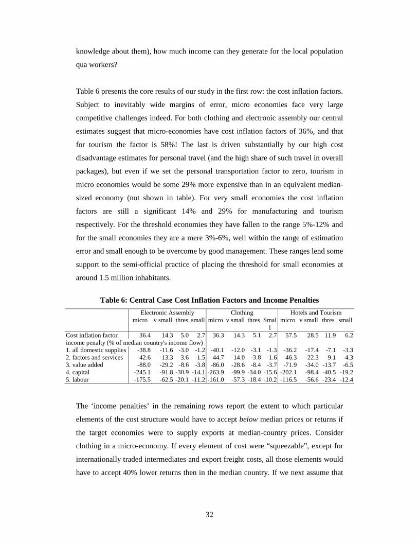
32

knowledge about them), how much income can they generate for the local population

qua workers?

Table 6 presents the core results of our study in the first row: the cost inflation factors.

Subject to inevitably wide margins of error, micro economies face very large

competitive challenges indeed. For both clothing and electronic assembly our central

estimates suggest that micro-economies have cost inflation factors of 36%, and that

for tourism the factor is 58%! The last is driven substantially by our high cost

disadvantage estimates for personal travel (and the high share of such travel in overall

packages), but even if we set the personal transportation factor to zero, tourism in

micro economies would be some 29% more expensive than in an equivalent median-

sized economy (not shown in table). For very small economies the cost inflation

factors are still a significant 14% and 29% for manufacturing and tourism

respectively. For the threshold economies they have fallen to the range 5%-12% and

for the small economies they are a mere 3%-6%, well within the range of estimation

error and small enough to be overcome by good management. These ranges lend some

support to the semi-official practice of placing the threshold for small economies at

around 1.5 million inhabitants.

Table 6: Central Case Cost Inflation Factors and Income Penalties

Electronic Assembly Clothing Hotels and Tourism micro v small thres small micro v small thres Smal

l micro v small thres small

Cost inflation factor 36.4 14.3 5.0 2.7 36.3 14.3 5.1 2.7 57.5 28.5 11.9 6.2 income penalty (% of median country's income flow) 1. all domestic supplies -38.8 -11.6 -3.0 -1.2 -40.1 -12.0 -3.1 -1.3 -36.2 -17.4 -7.1 -3.3 2. factors and services -42.6 -13.3 -3.6 -1.5 -44.7 -14.0 -3.8 -1.6 -46.3 -22.3 -9.1 -4.3 3. value added -88.0 -29.2 -8.6 -3.8 -86.0 -28.6 -8.4 -3.7 -71.9 -34.0 -13.7 -6.5 4. capital -245.1 -91.8 -30.9 -14.1 -263.9 -99.9 -34.0 -15.6 -202.1 -98.4 -40.5 -19.2 5. labour -175.5 -62.5 -20.1 -11.2 -161.0 -57.3 -18.4 -10.2 -116.5 -56.6 -23.4 -12.4

The ‘income penalties’ in the remaining rows report the extent to which particular

elements of the cost structure would have to accept below median prices or returns if

the target economies were to supply exports at median-country prices. Consider

clothing in a micro-economy. If every element of cost were “squeezable”, except for

internationally traded intermediates and export freight costs, all those elements would

have to accept 40% lower returns then in the median country. If we next assume that

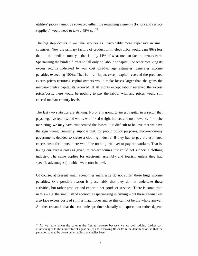
33

utilities’ prices cannot be squeezed either, the remaining elements (factors and service

suppliers) would need to take a 45% cut.25

The big step occurs if we take services as unavoidably more expensive in small

countries. Now the primary factors of production in electronics would earn 86% less

than in the median country – that is only 14% of what median factors owners earn.

Specialising the burden further to fall only on labour or capital, the other receiving its

excess returns indicated by our cost disadvantage estimates, generates income

penalties exceeding 100%. That is, if all inputs except capital received the predicted

excess prices (returns), capital owners would make losses larger than the gains the

median-country capitalists received. If all inputs except labour received the excess

prices/costs, there would be nothing to pay the labour with and prices would still

exceed median-country levels!

The last two statistics are striking. No one is going to invest capital in a sector that

pays negative returns, and while, with fixed weight indices and no allowance for niche

marketing, we may have exaggerated the losses, it is difficult to believe that we have

the sign wrong. Similarly, suppose that, for public policy purposes, micro-economy

governments decided to create a clothing industry. If they had to pay the estimated

excess costs for inputs, there would be nothing left over to pay the workers. That is,

taking our excess costs as given, micro-economies just could not support a clothing

industry. The same applies for electronic assembly and tourism unless they had

specific advantages (to which we return below).

Of course, at present small economies manifestly do not suffer these huge income

penalties. One possible reason is presumably that they do not undertake these

activities, but rather produce and export other goods or services. There is some truth

in this – e.g. the small island economies specialising in fishing – but these alternatives

also face excess costs of similar magnitudes and so this can not be the whole answer.

Another reason is that the economies produce virtually no exports, but rather depend

25 As we move down the column the figures increase because we are both adding further cost disadvantages to the numerator of equation (2) and removing flows from the denominator, so that the penalties have to be borne on a smaller and smaller base.

34

on remittances, aid or asset returns to fund essential imports26. The third possibility is

that preferences on their exports or product differentiation into niche markers allow

them to earn prices above those of the median country, or that they have benefactors

who will accept below market rates of return on their capital, or labour in return for

various non-pecuniary benefits of living in a small economy. Finally, regulation may

be more flexible and more cheaply achieved in small economies than in large ones

leaving more surplus for real incomes. This continuing advantage is independent of

the trading regime they face and so is not vulnerable to removal. Equally, however, it

can not be expanded to compensate for any loss of trading advantages as, say,

preferences are eroded.

The calculation of these income penalties is apparently an exercise in absolute

advantage – we are calculating whether the illustrative activities are viable at existing

exchange rates and factor rewards. Thus, the question arises of whether, if the

advantages that sustain current activities were eliminated, wages would fall far

enough to render them or some other activity viable. We have argued above that all

significant alternative activities face these sorts of excess costs, so comparative

advantage is not really the critical concept. Rather we should think about the question

in terms of the current illustrative activities. But even allowing wages and the prices

of services to fall to median-country levels and so treating traded goods and utilities

as the only things subject to the disadvantage of smallness, incomes would still need

to be 42-46% below those in the median country (income penalty concept 2 from

table 6). In fact, even with lower wages the quality-adjusted prices of services would

not fall that far, so the cut in incomes would need to be larger. Thus even allowing for

general equilibrium effects and for any benefits that comparative advantage could

bring, the fundamental issue is the absolute one: facing unavoidable excess real costs

of smallness, very small economies would be able to generate only very low real

incomes.

In WM we conduct extensive sensitivity tests on these results and find them robust

with respect to changes in weights. Clearly they are linear in the cost disadvantage

ratios. The most sensitive issue is the transportation cost factor because it is applied to

26 It is well-known, for example, that aid per head is much higher for small economies than for large

35

the full value of the export and, for tourism, to 25% of the value of a package. This is

clearly an area towards which both future research and policy consideration should be

directed.

7. Policy Implications

The message of this paper is robust and stark. While circumstances vary by economy

and class of economy it is clear that, on average, micro and very small economies face

huge competitive challenges. These economies will not be suitable locations for

industry or even tourism unless they have very specific advantages that allow them to

charge substantially higher prices than the median country. For hotels and tourism the

attractions of small tropical islands are plausible and we do, indeed, see viable tourist

industries on them27 Our results merely indicate that they will need to manage costs

carefully and will never achieve mass market penetration.

For manufacturing, on the other hand, the barriers look very high indeed, and if we

wish such industries to develop, the leverage of any corrective policies will need to be

correspondingly high. One common response is that since the costs of trading are so

high, small countries need the right to protect their industries. This is completely mis-

guided. The problem is not that that imports can get in too easily but the very

opposite. Adding barriers to trade will exacerbate not relieve problems of smallness.

Even where local industries could be successfully established behind tariff walls there

is nothing in the foregoing analysis to suggest that such an approach would be

economically beneficial. The theoretical discussion above showed that following

comparative advantage maximised real income: only not sufficiently to provide an

adequate income.

A related response has been to suggest subsidising business investment in order to

overcome the cost disadvantages of smallness. There are many arguments in the

policy-making literature for subsidising business in any economy. We do not accept

them, but, even if we did, the point to make here is that smallness adds nothing to

ones.

36

them. If you would not subsidise business in a large economy, neither should you do

so in an equivalent small one, for precisely the reasons outlined in the previous

paragraph. Smallness does not introduce marginal distortions that need to be

countervailed, but an overall feasibility constraint. If income is insufficient when you

maximise it, it will certainly be insufficient if you do not; and in the absence of the

market failures usually adduced to justify subsidies offering support to manufacturing

puts you in the latter category.

The conclusion must be that if unviable economies are to be made viable, an

additional source of income must be found and, presuming the absence of free

technological or organisational lunches, that means from abroad28. One source

internal to the set of small economies themselves is to economise on the costs of

economic management or even of statehood. Andriamananjara and Schiff (2001) and

Schiff and Winters (2003) argue strongly that by combining various functions of

government small states can both economise on costs and, possibly, exert a greater

influence on their environments. Whether such efficiencies are sufficient to overcome

the disadvantages we have noted here, we rather doubt, but there is undoubtedly a

case for seeking such efficiency gains in any case. We also note that in the cases

where smallness appears not to matter – e.g. Luxembourg, Liechtenstein, Andorra –

the secret appears to be to integrate extremely closely with the neighbouring large

countries.

In the end, however, we suspect that the sources of income to keep large small

economies going must be external – that ultimately the international community will

have to provide the compensating flows. Merely subsidising capital costs will not

generally be sufficient – there are too many other continuing disadvantages. Thus,

while international capital transfers – either bilateral or via international financial

institutions and development banks – will clearly help to reduce costs by improving

infrastructure and perhaps utilities, most of the disadvantages we see above are on the

current account – e.g. shipping costs, thin markets for skills etc. The most favourable

case for infra-structured salvation is probably communications links. If these are

27 See Briguglio et al. (1996) 28 Our brief discussion of policy certainly did not suggest that the disadvantages of smallness stemmed from policy inadequacy.

37

excellent and cheap, services relying on electronic interchange may become

competitive. But even so, the costs of importing goods will still be high and even in

‘electronic services’ personal contacts are important so small remote economies will

be disadvantaged to the high travel costs and long travel times. Thus, we believe that

one needs continuing current transfer to confer lasting viability.

One superficially promising route is via some sort of preferences for small countries’

exports, allowing them to sell at tariff-inclusive prices in industrial country markets

rather than world prices. This source of rent has historically been very important – as,

for example, with banana or tuna exports to the EU or clothing exports from the

Caribbean to the USA. The problems are first that other developing countries have

become more hostile to these preferences, as with Latin American challenges to

banana preferences and East Asian challenges to those on tuna, and that the more

legalistic regime of the WTO makes them far harder to defend than they were under

the GATT. Second, that as donors discover new favourites the preferences of the old

are eroded: consider Pakistan’s recent advantages under the textile quotas and the way

in which NAFTA and now AGOA reduced the advantages of the CBI. Third,

industrial countries wish, or perhaps are under pressure, to liberalise their trade

regimes anyway, so that the benefits of preferences are gradually declining and highly

insecure. In all these cases, as rents are reduced, very small economies face large

income penalties. A salutary thought is that if very small economies are dependent on

rents, the erosion of legal rents could presage a search for less social sources. Very

small countries are inherently difficult to police if their governments are not

sympathetic to global objectives.

An alternative route could be for industrial countries to subsidise small country trade

explicitly – either their exports or their imports or both. This would require conscious

policy-shifts in the major capitals and also derogations from WTO agreements. A

similar route would be straight income transfers (de Vries, 1975). In either case the

issue for the recipients would be the security of such transfers. As we noted above, we

believe that they would need to be permanent and so could not be dressed up merely

as transitional financing to encourage structural adjustment.

38

Explicit subsidies to micro and very small economies raise their own very particular

political challenges. Specifically, many of the cost disadvantages we have identified

must also apply to insular or isolated parts of larger countries. These disadvantaged

regions are often subsidised via regional policies, as for example, in the UK, Europe

more generally and China. But if small economies were permitted to have export

subsidies, one would need to argue why this privilege should not be extended to parts

of larger economies, for if it were it would probably fatally undermine subsidies

discipline in the WTO. The reason is not hard to formulate, but it may be

uncomfortable: within a country, people can move out of uneconomic locations.

Ultimately we must face the possibility that if the current preferences that small

countries receive are eroded and we do not somehow support their incomes in other

ways, many of their inhabitants will seek to work abroad. We have argued elsewhere

that liberalising the temporary movements of labour within the world economy –

mode 4 of the GATS – promises huge economic gains - Winters et al. (2003a, b). This

could be a key factor for very small economies, essentially allowing residents to earn

abroad but live and consume at home. Temporary workers from small countries would

still be at a disadvantage relative to those from larger ones: they would face higher

transport costs, less effective networks for finding jobs and easing migratory strains,

and higher consumption costs at home. However, particularly if they had preferential

access – e.g. guaranteed quotas – the benefits would be large enough to cover the

disadvantages. But again the sustainability of preferences would fall under question.

The alternative to temporary mobility would be permanent migration. In the current

political climate this touches raw nerves on of both sides: of immigration in most

developed countries and of depopulation, and maybe eventual cultural extinction, in

the very small economies29.

The title of Easterly and Kraay’s (2000) important paper ‘Small countries, small

problems’ upset many commentators on the problems of small size: the problems,

they say, are very large if you face them. But the title contains a silver lining: ‘small

problems, small solutions’. Particularly if we limit transfers to the micro and very

small economies they will need to be only very small in aggregate – small amounts of

39

money, small flows of people etc. If there is a political will to offer them – not only in

the developed, donor, countries but also among developing countries, especially those

just too big to receive them – they would be perfectly manageable. Around 3.12

million people (0.05% of the world’s population) live in countries of below 200

thousand population, 6.31 million (0.10%) in those below 400 thousand and 28.20

million (0.45%) in those below 1.5 million population. These are not insurmountable

by any yardstick.

Annexes

Annex 1: Sample of Countries

Anguilla Gabon Netherlands Sweden Antigua &Barbuda Germany New Zealand Taiwan Argentina Greece Nigeria Tanzania Australia Grenada Niue Thailand Austria Guyana Norway Tonga Bangladesh Hong Kong Pakistan Trinidad & Tobago Barbados Hungary Palau Turkey Belgium India Papua New Guinea Tuvalu Belize Indonesia Peru Uganda Botswana Ireland Philippines United Kingdom Brazil Italy Poland United States Cameroon Jamaica Portugal Uruguay Canada Japan Samoa Vanuatu Chile Kenya Senegal Venezuela China Kiribati Seychelles Vietnam Colombia Lesotho Singapore Zambia Cook Islands Malawi Solomon Islands Zimbabwe Cote d'Ivoire Malaysia South Africa Czech Republic Marshall Islands South Korea Denmark Mauritius Spain Dominica Mexico Sri Lanka Ecuador Micronesia St Kitts and Nevis Fiji Mozambique St. Vincent &

The Grenadines

Finland Namibia Suriname France Nauru Swaziland

Annex 2: The Continuous Variables from the Survey

Airfreight ▪ Airfreight costs of transporting 100 kilograms of general cargo “to” and “from” London, Tokyo and New York.

Sea freight ▪ Shipping costs of transporting a standard 20ft Full Container Load (FCL) 29 This scenario also shows why subsidising human capital formation is at best a very partial answer for very small economies: the highly skilled will leave, returning the small economy to square one.

40

of general cargo “to” and “from” Rotterdam, Yokohama and New York. Wages ▪ Average hourly wage for unskilled jobs (3) and annual salary for the rest

(8). Telephone ▪ Rate per minute of local calls during peak hour

▪ Rate per minute of international calls during peak hour ▪ Installation fee for a standard commercial line ▪ Line rental fee for a standard commercial line

Electricity ▪ Costs of electricity for a standard commercial line (KWh) ▪ Connection fee for a standard commercial line

Water ▪ Costs of water for standard commercial rate (per 1000 litres) ▪ Standard commercial connection fees

Fuel ▪ Retail price of diesel per litre ▪ Retail price of petrol per litre

Land ▪ Average annual cost of per square metre of industrial (factory) space (average industrial estate) ▪ Average annual rent of per square metre of office space in the prime location

Bank ▪ Prime commercial bank lending interest rate ▪ Prime commercial bank deposit interest rate

Corporate Tax ▪ Corporate tax rate for residents ▪ Corporate tax rate for non-residents

Import Duties ▪ Un-weighted average (nominal) tariff rate ▪ Import weighted (nominal) tariff rate ▪ Receipts from import duties and taxes (including custom duties, VAT, sales taxes, supplementary duties, etc) as percentage of total government tax revenues as available for the latest year

Personal Air Travel

▪ Cost of economy return from London, Tokyo or New York (separate source)

Note: The data on passenger travel costs were obtained from the Commonwealth Secretariat’s travel agents. They represent the cost of an economy return ticket from each capital to the respective destination.

Annex 3: The Categorical Variables from the Survey

Are unskilled/semi-skilled/skilled workers domestically available or do they have to be hired from abroad?

(1) Domestically available and there is no need to import them from abroad. (2) There are enough workers domestically available to satisfy most of the demand; however occasionally workers need to be imported from abroad. (3) Workers are available domestically, but many need to be imported from abroad to satisfy demand (4) Some workers are domestically available, but most need to be imported from abroad (5) Few workers are available domestically. The vast majority of workers are imported from abroad

How long does it take to get a new connection?

(1) <72 hours, (2) < 1 week, (3) 1 week - 1 month, (4) >1 month, (5) Not available (i.e., indefinite delays)

How frequently does one experience disruptions?

(1) No disruption, (2) Very rare, (3) Rare, (4) Quite frequently (5) Most frequently

How long does it take, in general, to have a broken line repaired?

(1) 48 hours, (2) 5 working days, (3) 2 weeks, (4) > 2 weeks

41

(Telephone only) Are tax incentives available for exporters and other businesses?

YES/NO

Export duty rate (duties from exports as percentage of total government tax revenues)

Converted into YES/NO since there were too few values (different from 0) to run a regression.

Is there a special exchange rate for exports?

YES/NO

References:

Alesina, A. and Spolaore, E. (2004), ‘The Size of Nations MIT Press, Cambridge,

Mass.

Andriamananjara, S. and Schiff, M. (2001) 'Regional Cooperation Among

Microstates', Review of International Economics, Vol. 9 (1), pp. 42-51

Armstrong, H., De Kervenoael, R., Li, X. and Read, R. (1998), ‘A Comparison of the

Economic Performance of Different Micro-states, and Between Micro-states and

Larger Countries’, World Development, Vol. 26 (4), pp. 639-656

Atkins, J.P., Mazi, S. and Easter, C.D (2001), ‘Small States: A Composite

Vulnerability Index’, in Peretz, Faruqi and Kisanga (eds.). Small States in the Global

Economy, Commonwealth Secretariat.

Banerji, R. (1978), ‘Average Size of Plants in Manufacturing and Capital Intensity,

Journal of Development Economics, Vol. 5, pp. 155-61

Bera, A.K. and C.M. Jarque (1981), 'An Efficient Large-Sample Test for Normality of

Observations and Regression Residuals', Australian National University Working

Papers in Econometrics, 40, Canberra

Breusch, T. S. and Godfrey, L. G. (1981) ‘A review of recent work on testing for

autocorrelation in dynamic simultaneous models’, in Currie D, Nobay R, and Peel D

42

(ed.s) Macroeconomic Analysis: Essays in Macroeconomics and Econometrics,

London, Croome Helm, pp. 63-105

Briguglio, L. (1995), ‘Small Island Developing States and Their Economic

Vulnerabilities’, World Development, Vol. 23 (9), pp.1615-1632

Briguglio, L., B. Archer, J. Jafari and G. Wall (1996) Sustainable Tourism in Islands

and Small States: Issues and Policies. London: Cassel-Pinter

Briguglio, L. (1998) ‘Small Country Size and Returns to Scale in Manufacturing’,

World Development, Vol 26 (3), pp. 507-15

Chow, G. C. (1960), 'Test of Equality Between Sets of Coefficients in Two Linear

Regressions', Econometrica, 28, pp. 591-605

Codrington, H. (1989), ‘Country Size and Taxation in Developing Countries’, Journal

of Development Studies, 25 (4), pp. 508-20

de Vries, B.A. (1975) ‘Development Aid to Small Countries’ in Selwyn, P. (ed.),

Development Policy in Small States. London: Croom Helm Ltd

Dornbusch, R., Fischer, S. and Samuelson, P. (1977) ‘Comparative Advantage, Trade,

and Payments in a Ricardian Model with a Continuum of Goods’, American

Economic Review, Vol. 67 (5) pp. 823-39

Easterly, W. and Kraay, A. (2000) ‘Small States, Small Problems? Income, Growth,

and Volatility in Small States’, in World Development, Vol. 28 (11), pp. 2013-2027

Hummels, D. (1999) ‘Toward a Geography of Trade Costs?’, mimeo, University of

Chicago

Jansen, M. (2004) ‘Income Volatility in Small and Developing Economies: export

concentration matters,’ Discussion Paper No. 3:1-35, World Trade Organization,

Geneva.

43

Limao, N. and Venables, A. J. (2001) ‘Infrastructure, Geographical Disadvantage,

Transport Costs, and Trade’, World Bank Economic Review, Vol. 15 (3), pp. 451-79

Kuznets, S. (1960) ‘Economic Growth of Small Nations’, in Robinson, E. A.G. (ed.)

The Economic Consequences of the Size of Nations: Proceedings of a Conference

held by the International Economic Association. London: MacMillan

Pryor, F.L. (1972) ‘The size of production establishments in manufacturing’,

Economic Journal, Vol. 82, pp. 547-566

Ramsey, J.B. (1969), ‘Test for Specification Errors in Classical Linear Least Squares

Regression Analysis', Journal of the Royal Statistical Society, B, 31, pp. 350-71

Redding, S. and Venables, A. (2002a) The Economics of Isolation and Distance.

Mimeo, Commonwealth Secretariat.

Redding, S. and Venables, A. (2002b) Economic Geography and International

Inequality, CEPR Discussion Paper No. 2568

Robinson, E. A. G. (1960) The Economic Consequences of the Size of Nations:

Proceedings of a Conference held by the International Economic Association.

London: MacMillan

Schiff, M. and Winters, L. A. (2003) Regional Integration and Development, Oxford

University Press for World Bank.

Srinivasan, T. N. (1986) “The Costs and Benefits of Being a Small, Remote, Island,

Landlocked, or Ministate Economy” World Bank Research Observer Volume: 1

(1986) Issue: 2, pp.205-18.

Vamvakidis, A. (1998) ‘Regional Trade Agreements or Broad Liberalization: Which

Path Leads to Faster Growth?’ IMF Staff Papers, Volume 46, No. 3 (September/

December 1999)

44

Winters, L. .A and Martins, P. M. G. (2004) Beautiful but Costly: Business Costs in

Small Economies, mimeo, Department of Economics, University of Sussex, to be

published by Commonwealth Secretariat.

Winters, L. A., Walmsley, T., Wang, Z., and Grynberg, R. (2003) ‘Negotiating the

temporary movement of natural persons: an agenda for the Development Round’, The

World Economy, Vol. 26 (8), pp. 1137-1162